| Issue |
A&A
Volume 689, September 2024
|
|
|---|---|---|
| Article Number | A191 | |
| Number of page(s) | 10 | |
| Section | Astrophysical processes | |
| DOI | https://doi.org/10.1051/0004-6361/202450441 | |
| Published online | 12 September 2024 | |
Timing irregularities and glitches from the pulsar monitoring campaign at IAR
1
Instituto Argentino de Radioastronomía (CCT La Plata, CONICET; CICPBA; UNLP), C.C.5, (1894) Villa Elisa, Buenos Aires, Argentina
2
Facultad de Ciencias Astronómicas y Geofísicas, Universidad Nacional de La Plata, Paseo del Bosque, B1900FWA La Plata, Argentina
3
Department of Space, Earth and Environment, Chalmers University of Technology, 412 96 Gothenburg, Sweden
4
Instituto de Astronomía Teórica y Experimental, CONICET-UNC, Laprida 854, X5000BGR Córdoba, Argentina
5
Facultad de Matemáitica, Astronomía, Física y Computación, UNC. Av. Medina Allende s/n, Ciudad Universitaria, X5000HUA Córdoba, Argentina
6
School of Mathematical Sciences, Sciences Rochester Institute of Technology Rochester, NY 14623, USA
7
Center for Computational Relativity and Gravitation, Rochester Institute of Technology, 85 Lomb Memorial Drive, Rochester, NY 14623, USA
8
Departamento de Física, Universidad de Santiago de Chile (USACH), Av. Víctor Jara 3493, Estación Central, Chile
9
Center for Interdisciplinary Research in Astrophysics and Space Sciences (CIRAS), Universidad de Santiago de Chile, Santiago de Chile, Chile
Received:
18
April
2024
Accepted:
21
June
2024
Abstract
Context. Pulsars have a very stable rotation overall. However, sudden increases in their rotation frequency, known as glitches, perturb their evolution. While many observatories commonly detect large glitches, small glitches are harder to detect because of the lack of daily cadence observations over long periods of time (years).
Aims. We aim to explore and characterise the timing behaviour of young pulsars on daily timescales, looking for small glitches and other irregularities, in order to further our comprehension of the real distribution of glitch sizes. Our findings have consequences for the theoretical modelling of the glitch mechanism.
Methods. We observed six pulsars with up to daily cadence between December 2019 and January 2024 with the two antennas of the Argentine Institute of Radio Astronomy (IAR). We used standard pulsar timing tools to obtain the times of arrival of the pulses and to characterise the pulsar’s rotation. We developed an algorithm to look for small timing events in the data and calculate the changes in the frequency (ν) and its derivative (ν̇) at those epochs.
Results. We find that the rotation of all pulsars in this dataset is affected by small step changes in ν and ν̇. Among them, we find three new glitches that have not been reported before: two glitches in PSR J1048−5832 with relative sizes of Δν/ν = 9.1(4)×10−10 and Δν/ν = 4.5(1)×10−9, and one glitch in the Vela pulsar with a size of Δν/ν = 2.0(2)×10−10. We also report new decay terms on the 2021 Vela giant glitch, and on the 2022 giant glitches in PSR J0742−2822 and PSR J1740−3015, respectively. In addition, we find that the red noise contribution significantly diminished in PSR J0742−2822 after its giant glitch in 2022.
Conclusions. Our results highlight the importance of high-cadence monitoring with an exhaustive analysis of the residuals to better characterise the distribution of glitch sizes and to deepen our understanding of the mechanisms behind glitches, red noise, and timing irregularities.
Key words: methods: observational / pulsars: general
Corresponding author; This email address is being protected from spambots. You need JavaScript enabled to view it. .
© The Authors 2024
 Open Access article, published by EDP Sciences, under the terms of the Creative Commons Attribution License (https://creativecommons.org/licenses/by/4.0), which permits unrestricted use, distribution, and reproduction in any medium, provided the original work is properly cited.
This article is published in open access under the Subscribe to Open model. This email address is being protected from spambots. You need JavaScript enabled to view it. to support open access publication.
1. Introduction
Pulsars are neutron stars that exhibit pulsed emission, primarily in radio frequencies. Their extremely high moment of inertia provides them with exceptionally stable rotation, which positions some pulsars among the most stable clocks in the Universe (Hobbs et al. 2012). If a pulsar is isolated, the evolution of its rotation is relatively smooth, decelerating steadily as a result of energy loss via dipole emission. However, dynamic effects may perturb this evolution, primarily in young pulsars. These effects are known as glitches and timing noise (Lorimer & Kramer 2004).
Glitches are discrete events consisting of a sudden change in rotation frequency, most often accompanied by a sudden change in the frequency derivative, which typically returns to its preglitch value exponentially (Zhou et al. 2022b). At present, more than 200 pulsars are known to present glitches1 (Espinoza et al. 2011; Fuentes et al. 2017; Manchester 2018; Basu et al. 2022). These are believed to be caused by decoupling between the superfluid interior of the star and the solid crust (Baym et al. 1969; Haskell & Melatos 2015; Gügercinoğlu et al. 2022). The magnitude of the glitches provides insight into the reservoir of angular momentum accessible in the superfluid interior (Zhou et al. 2022a). Glitch sizes, characterised by the relative jump in their spin frequency (Δν/ν), exhibit a bimodal distribution (Espinoza et al. 2011; Yu et al. 2013), separating glitches (Fuentes et al. 2017) into giant glitches (Δν/ν ∼ 10−6) and small glitches (Δν/ν ∼ 10−9).
On the other hand, timing noise manifests itself as a smooth and wandering behaviour around a simple rotational evolution, and its explanation remains a puzzle (Hobbs et al. 2010; Parthasarathy et al. 2019). It is unknown whether timing noise may have similar causes, such as superfluid turbulence (Melatos & Warszawski 2009) or unresolved microglitches (Janssen & Stappers 2006), stem from entirely different mechanisms, such as fluctuations of the magnetosphere (Lyne et al. 2010), or arise from the combination of internal superfluid torque and external magnetospheric torque (Antonelli et al. 2023).
Although the distinction between timing noise and glitches is evident in terms of the discreteness of the event (Shannon et al. 2016), the smallest glitches can often be mistaken for timing noise and vice versa (Grover et al. 2024). In particular, even though low sensitivity can also obscure detections, the main cause of the confusion between a glitch-like event and timing noise is that the monitoring cadence is often too low to evaluate the discreteness of the event. Therefore, by exploring the distribution of small irregularities in pulsar timing with high-cadence observations, more information can be obtained about the connection or difference between glitches and timing noise.
Our Pulsar Monitoring in Argentina2 (PuMA) collaboration has been observing a set of bright pulsars in the southern hemisphere since 2019 (Gancio et al. 2020; Lousto et al. 2024) using the 30m antennas of the Argentine Institute of Radioastronomy (IAR). In particular, we have been closely monitoring the millisecond pulsar PSR J0437−4715 (Sosa Fiscella et al. 2021a), the magnetar XTE J1810−197 (Araujo Furlan et al. 2024), and seven pulsars that have previously exhibited glitches: PSR J0742−2822, PSR J0835−4510 (also known as the Vela pulsar; Lousto et al. 2022), PSR J1048−5832, PSR J1644−4559, PSR J1721−3532, PSR J1731−4744, and PSR J1740−3015. Previous results from this campaign include: (i) the confirmation of a glitch in PSR J0742−2822 (Zubieta et al. 2022a; ii) the confirmation of the 2019 glitch in the Vela pulsar (Lopez Armengol et al. 2019) and the announcement of its 2021 glitch (Sosa-Fiscella et al. 2021b; Zubieta et al. 2024b), which we observed only one hour after it occurred; (iii) the report of a glitch in PSR J1740−3015 that occurred in late 2022 (Zubieta et al. 2022b); (iv) the report of two small glitches in PSR J1048−5832 (Zubieta et al. 2023), later confirmed by Liu et al. (2023); and (v) the detection of the largest glitch reported to date in PSR J1048−5832 (Zubieta et al. 2024a). Concerning the remaining pulsars (PSR J1644−4559, PSR J1721−3532 and PSR J1731−4744), none of them have exhibited large glitches since the beginning of our monitoring campaign.
Most giant glitches are characterised by a positive jump in frequency (Δν > 0) and a negative jump in the spin-down ( ). However, smaller events can present every combination of these signs (Espinoza et al. 2021), and they may actually be small glitches, part of the timing noise, or some other phenomenon. Unfortunately, the statistics of these events are poor, as they are difficult to detect with low-cadence monitoring. In this work, we present a timing dataset of six pulsars in Sect. 2 observed from the IAR with up to daily cadence. In Sect. 3, we explain the algorithm we developed to perform a systematic search for small discrete events with all the possible combinations of signs in Δν and
  in the timing data of the pulsars. We present the results in Sect. 4, where we show the detected events and classify three of them as glitches after a more thorough analysis. In addition, in Sect. 4 we explore the timing data for pulsars for which we already reported giant glitches in order to look for new recovery terms. We conclude with a discussion of our results in Sect. 5 and with some final remarks in Sect. 6.
2. Pulsar glitch monitoring program at IAR
2.1. Observations
The IAR observatory, located near the city of La Plata, Argentina, has two 30m single-dish antennas, “Carlos M. Varsavsky” (A1) and “Esteban Bajaja” (A2). The former is configured to observe at a central frequency of 1400 MHz with a bandwidth of 112 MHz and one circular polarisation, while the latter observes at a central frequency of 1428 MHz with a bandwidth of 56 MHz and two circular polarisations3.
Since 2019, the PuMA collaboration has been using both antennas to observe a set of eight pulsars and one magnetar with up to daily cadence4. In this work, we exclude the millisecond pulsar PSR J0437−4715 –which has an extremely stable rotation–, the pulsar PSR J1721−3532, and the magnetar XTE J1810−197, as the timing accuracy achieved for them is only suitable for the detection of giant glitches (Araujo Furlan, in prep.). The number of observations collected for this work and their typical durations are shown in Table 1. This dataset includes all available observations up to January 5, 2024.
Observations analysed in this work.
For all observations, we used the PRESTO package (Ransom et al. 2003; Ransom 2011) to remove radio-frequency interferences (RFIs) with the task rfifind and to fold the observations with the task prepfold. The times of arrival (TOAs) were then calculated using the Fourier phase gradient-matching template fitting method described by (Taylor 1992), implemented in the pat package in psrchive (Hotan et al. 2004). Given their similarities, we used the same template for observations of both antennas. We constructed this template by employing a smoothing wavelet technique (psrsmooth package in psrchive) on the pulse profile of a high-signal-to-noise-ratio(S/N) observation that was not part of the subsequent timing analysis.
2.2. Pulsar timing
Pulsar rotation is tracked by monitoring the TOAs of the pulses, while a timing model is developed to predict the expected TOAs.
In the timing model, a Taylor expansion is used to model the temporal evolution of the pulsar phase,
 (1)
(1)
where ν,  and
and  are the rotation frequency of the pulsar, and its first and second derivatives, respectively, and t0 is the reference epoch. Diverse physical phenomena can be studied through this technique, including the internal structure of pulsars, the characteristics of which are thought to give rise to glitches (Antonopoulou et al. 2022).
During a glitch, there is a sudden jump in the pulsar rotation frequency. The additional phase induced by a glitch can be described as (Yu et al. 2013):
![Mathematical equation: $$ \begin{aligned} \phi _{\mathrm{g} }(t) = \Delta \phi + \Delta \nu _{\mathrm{p} }&(t-t_{\mathrm{g} }) + \frac{1}{2} \Delta \dot{\nu }_{\mathrm{p} } (t-t_{\mathrm{g} })^2 +\nonumber \\&\frac{1}{6} \Delta \ddot{\nu }(t-t_{\mathrm{g} })^3 + \left[1-\exp {\left(-\frac{t-t_{\mathrm{g} }}{\tau _{\mathrm{d} }}\right)} \right]\Delta \nu _{\mathrm{d} } \, \tau _{\mathrm{d} }, \end{aligned} $$](/articles/aa/full_html/2024/09/aa50441-24/aa50441-24-eq8.gif) (2)
(2)
where tg denotes the glitch epoch, Δϕ counteracts the uncertainty on tg, and Δνp,  , and
, and  are the respective permanent shifts in ν,
  and
and  , respectively, relative to the preglitch solution. Additionally, Δνd stands for the temporary increase in frequency that recovers exponentially over the duration of τd. Considering the instantaneous frequency shift as Δνg = Δνp + Δνd and the instantaneous shift in the frequency derivative as
  , one can compute the recovery coefficient, Q, which relates the temporary and permanent frequency shifts as Q = Δνd/Δνg, and the total instantaneous jumps in ν and
  as Δνg/ν and
  respectively.
Initially, we took the parameters for the timing models from the ATNF pulsar catalogue (Manchester et al. 2005a), and then we updated them by fitting our data to the timing model (Eq. 1) with the TEMPO2 (Hobbs et al. 2006) software package. Pulsars that present abundant timing noise or have undergone glitches could be difficult to solve coherently. However, the high cadence of our observations allows phase-connected timing solutions without adding additional phase jump.
2.3. Data release
We used our TOAs to update the ephemeris for each pulsar. The TOAs and up-to-date timing solutions can be found at our online repository5. The residuals for pulsars that have not undergone a giant glitch during our observation campaign before January 5 2024 (MJD 60314) are shown in Fig. 1. In Fig. 2 we show the residuals of pulsars with giant glitches that took place during our observation campaign.
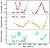 |
Fig. 1. Residuals for pulsars that did not have a giant glitch during our campaign. |
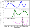 |
Fig. 2. Residuals for pulsars that experienced a giant glitch during our campaign. |
To account for jitter or systematic errors, we included the parameters EFAC and EQUAD, which model white noise by modifying each TOA uncertainty as
 (3)
(3)
where σi is the TOA uncertainty for each observation derived from the cross-correlation between the template profile and the folded observation. EFAC captures the impact of unaccounted-for instrumental effects and imperfect estimations of TOA uncertainties, while EQUAD addresses any additional sources of time-independent uncertainties, such as pulse jitter.
To obtain EFAC and EQUAD for each pulsar, we fitted ν and  in a data span that is sufficiently short to obtain flat residuals, as shown in Fig. 3. We then used TempoNest (Lentati et al. 2014) to obtain the white noise of the pulsar.
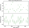 |
Fig. 3. Process to adjust the TOA uncertainties. Top: We keep a short data span with flat residuals. Bottom: We add the parameters EFAC and EQUAD (Eq. 3) calculated with TempoNest. |
3. Timing irregularity detection
3.1. Search sensitivity
We estimated the detection limits for our results following Espinoza et al. (2014). When a positive frequency jump (i.e. glitch) occurs, the residuals start to diverge linearly towards negative values. Then, if there is also a negative change in the spin-down rate, the residuals gradually rise towards positive values with a parabolic behaviour. This behaviour is depicted in Figure 4.
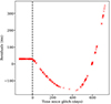 |
Fig. 4. Signature of a glitch with Δν > 0 and |

To ensure the detection of a glitch, the cadence of the observations must be high enough to have at least one TOA before the residuals become positive again. Additionally, the most negative residual value must exceed the TOA uncertainties. Consequently, we define our detection boundaries for events with Δν > 0 and  using the following equation, which accounts for both conditions:
 (4)
(4)
This criterion is also applicable to events with Δν < 0 and  . We assume a daily monitoring cadence (ΔT = 1 d) in the analysis of Sect. 4.
On the other hand, for events where Δν and  have the same sign, the only criterion is that the TOA uncertainties should be smaller than the residuals. Considering these criteria and Eq. (4), we can define our sensitivity in detecting events with any combination of signs. In our observations, we find that the detection limit for cases with different signs in Δν and
  is primarily determined by the uncertainties associated with the TOAs, rather than the observation cadence.
3.2. Method
During a glitch, there is a sudden positive jump in ν. In this case, residuals after the glitch diverge linearly to negative values, and they recover quadratically if there is also a discontinuous change in  of the opposite sign. In the case of an anti-glitch, the jump in ν is negative and the change in
  is positive, and so residuals diverge linearly to positive values and then recover quadratically. Hence, one method for glitch detection is to set t0 at the suspected glitch epoch and to fit ν and
  to the data before and after t0; we denote the values fitted to the data after t0 as ν′ and
  . The comparison between ν and ν′ can reveal the presence of a glitch.
We developed an algorithm based on PINT (Luo et al. 2021, 2019) to look for discrete jumps in frequency in our pulsar timing data6. The algorithm works as follows (see Fig. 5 for a schematic representation):
-
Restrict the timing data to a small data span of 2L days and set the parameter t0 (see Eq. 1) at the middle of that data span. That is, for a data span [MJD X, MJD X+2L], define ti= MJD X+L and set t0 = ti.
-
If the number of TOAs in [MJD X, MJD X+L] or [MJD X+L, MJD X+2L] is lower than Nmin, go to step 6.
-
Fit ν and
 (with their uncertainties σν and
  ) using only TOAs within [MJD X, MJD X+L].
 -
Fit ν′ and
 (with their uncertainties σν′ and
  ) using only TOAs within [MJD X+L, MJD X+2L], keeping the value of t0 fixed.
 -
Calculate Δν = ν′−ν and
 . If |Δν|> σΔν, save the values Δν and
  .
. -
Repeat from 1 to 5 with [MJD X+1, MJD X+2L+1], and t0 = ti + 1 d.
-
Finally, if two detections are closer than L days, keep only the one with the highest value of |Δν|.
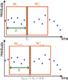 |
Fig. 5. Schematic representation of steps 1 and 2 of the algorithm described in Sect. 3.2. Example with Nmin = 5. Top: ν and |


Here, Nmin and L are user-specified parameters. We tested different values and conclude that L = 24 and Nmin = 6 offer a good compromise between having good statistics in each window and not averaging out small events. The minimum size of Δν that we can detect is defined by Eq. 4. We note that we keep  fixed at the value fitted with the whole data span.
4. Results
Figure 6 shows the detections associated with the six glitching pulsars. We excluded the detections of giant glitches in PSR J0742−2822, PSR J0835−4510, and PSR J1740−3015 in order to better visualise the distribution of smaller events detected. All of them were detected in quadrant IV, as is usual for giant glitches.
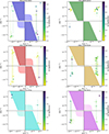 |
Fig. 6. Irregularities detected by our algorithm in the six pulsars. The colour bar indicates the significance of the detection. The two shaded regions correspond to detection limits following Eq. 4, calculated with σTOA and σTOA + ΔσTOA, respectively. |
To simplify the discussion, we refer to the top right quadrant in each plot (Δν,  ) as quadrant I, to the top left (Δν < 0,
  ) as quadrant II, to the bottom left (Δν,
  ) as quadrant III, and to the bottom right (Δν > 0,
  ) as quadrant IV. In addition to analysing the size distribution of events, we also studied each of them in detail. To change the status of an event to a glitch, we used the glitch plug-in in tempo2 (Hobbs et al. 2006) to subdivide the observations into blocks spanning between 6 and 10 days, ensuring that each block contains at least six TOAs, and then fitted ν0 and
  in each of these blocks. We classify an event as a glitch when we observe a step-like change in ν0 and the residuals cannot be adequately fitted using a second-order polynomial model, but instead require fitting with a step change function. If we do not detect a step-like change in ν0, we change the event status to irregularity.
To obtain detection limits, we used Eq. 4, considering the average of all σTOA for each pulsar and its standard deviation (ΔσTOA). We show these detection limits as shaded regions in Fig. 6, where the smaller regions were calculated with σTOA and the larger regions were calculated assuming σTOA + ΔσTOA.
4.1. PSR J0742–2822
We detected 13 events: 4 in quadrant I, 2 in quadrant II, 3 in quadrant III, and 4 in quadrant IV. Despite the significance of some events with Δν > 0 and  , we did not find glitch signatures in the residuals for any of them. We note that eight irregularities have Δν > 0, while only five have Δν < 0. These jumps in the rotation frequency are accompanied by opposite-signed, same-signed, or null alterations in
  . All events oscillate between 5 × 10⁻⁹ < |Δν(s−1)| < 2 × 10⁻⁷ and
  .
.
Our algorithm also detected the last giant glitch in PSR J0742−2822, which was excluded from Fig. 6. This glitch was initially reported by Shaw et al. (2022), and then we reported our confirmation (Zubieta et al. 2022a, 2023) of a giant glitch of Δνg/ν = 4295(1)×10−9 on MJD = 59839.4(5). However, our post-glitch data span was not sufficient to detect any long-term exponential recovery. In the current work, with a much longer post-glitch data span, we assume tg = 59839.4(5) as reported in (Basu et al. 2022)7 and we find one recovery term of τ = 33.4(5) d with a degree of recovery of Q = 0.446(1)%, as shown in Fig. 7. Also, using a combination of PINT (Luo et al. 2021) and an MCMC-like code to find the solutions, we calculated the evidence for a model considering a change in  and the evidence for one without it. The Bayes factor for the model with
  over the model without it yielded 1.2 × 10⁻⁸, which indicates that the model with
  is strongly preferred. The updated parameters considering the new recovery term can be seen in Table 2.
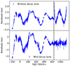 |
Fig. 7. Detection of a new decay term in the PSR J0742−2822 glitch on MJD 59839.4(5). Top: Residuals without considering any decay term. Bottom: Residuals considering one decay term of 33.4(5) d. |
Updated parameters for all glitches detected by PuMA collaboration between MJD 58832 and MJD 60411.
Figure 7 shows that the residuals flatten after the glitch once the glitch model has been subtracted. This has two strong implications: the post-glitch behaviour is explained with only one decay component of 33.4(5) d and the red noise component significantly diminishes after the glitch, at least for the 300d covered by our observations.
To quantify the change in red noise before and after the glitch, we explored the behaviour of  and
and  , subtracting the glitch model from the data. Following Arzoumanian et al. (1994), we also calculated the parameter
 ![Mathematical equation: $ \Delta_n(t) = \log{\left[ \lvert\ddot{\nu}\rvert t^3 / (6 \nu) \right]} $](/articles/aa/full_html/2024/09/aa50441-24/aa50441-24-eq55.gif) , where t ≃ 10n s. This parameter quantifies the strength of the timing noise. We adopted n = 7 and show the results in Fig. 8.
, where t ≃ 10n s. This parameter quantifies the strength of the timing noise. We adopted n = 7 and show the results in Fig. 8.
 |
Fig. 8. Timing parameters of J0742−2822 calculated in 100 d windows with consecutive windows overlapping by 50 TOAs; the time window is represented with a horizontal error bar. Top: Evolution of |


Figure 8 shows that the amplitude of the oscillations in  and
and  is larger pre-glitch than post-glitch. Also,
  stabilises around zero after the glitch, and the pre-glitch mean value of Δ7 is above the post-glitch mean value of Δ7, which indicates that the timing noise is stronger before the glitch.
4.2. PSR J0835–4510
PSR J0835−4510 (Vela pulsar) is the most studied pulsar in the southern hemisphere because of the periodicity of its giant glitches (∼3 yr). Our long observations of the bright Vela pulsar lead to events detected with a higher significance (up to 30σ), as seen in Fig. 6.
We detected 23 events. It is particularly interesting that, with the exception of two of them, all events are in the quadrants I or II, which means that most of the events have a positive  . After each giant glitch, Vela shows a negative jump in
  , which recovers exponentially at the beginning, and then linearly until a value near the pre-glitch value of
  is reached. At this point, another glitch is expected to occur (Gügercinoğlu et al. 2022). It may be that this positive trend (in which
  ) is not perfectly smooth and that there are instances where
  increases faster, thereby producing discrete events that are found by our method of detection. In particular, all events lie in the range of 6 × 10⁻¹⁰ < |Δν(s−1)| < 2 × 10⁻⁸ and
  .
.
Our algorithm also detected the 2021 Vela giant glitch, which we excluded from Fig. 6. We announced this glitch in Sosa-Fiscella et al. (2021b) and, later on, we reported the presence of two short exponential decay components associated with that giant glitch, namely τ1 = 6.400(2) d (with Q1 = 0.2(1)%) and τ2 = 0.994(8) d (with Q2 = 0.7(1)%), in Zubieta et al. (2023). Here we report the detection of a third recovery term with a much longer timescale of τ3 = 535(8) d, and a significant degree of recovery of Q3 = 41(1)%. We show the corresponding residuals in Fig. 9, and updated parameters for the glitch in Table 2.
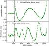 |
Fig. 9. Detection of a new decay term in the 2021 Vela glitch. Top: Residuals without considering long decay term. Bottom: Residuals considering the long decay term of 535(8) d. We note the much smaller residual scale. The signal that remains is the timing noise of the Vela pulsar. |
Between our 23 detections mentioned above, we detected a small event around MJD 59479, which is 62 days after the giant glitch. This event was initially fitted to quadrant I by the algorithm with a S/N of 34. A second, more dedicated analysis shows this event is a glitch. We find a best-fitting solution with  . This change of sign depends on factors such as the data span used for fitting the pre-glitch and post-glitch timing model, and the glitch epoch defined (not properly found by the algorithm). Therefore, it is essential to characterise glitches manually once they are detected by the automatic algorithm in order to derive more robust glitch parameters.
We analysed the residuals restricted to a data span of 30 d around the glitch in order to avoid the effects of the short exponential recoveries of the giant glitch (Zubieta et al. 2023). We show the associated residuals in Fig. 10, and summarise these results in Table 2. We defined tg halfway between the last pre-glitch observation and the first post-glitch observation. We note that this glitch has a typical signature of Δν > 0 and  but the magnitude of both of them is smaller than in giant glitches. This is the smallest glitch reported for the Vela pulsar so far.
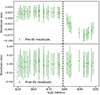 |
Fig. 10. Detection of a small glitch 62 days after the 2021 giant glitch. Top: Residuals without considering the small glitch. Bottom: Residuals after fitting for the small glitch. |
4.3. PSR J1048–5832
We detected a total of 14 events in this pulsar. It is seen from Fig. 6 that the events are more concentrated in quadrants II and III (nine events in total) than in I and IV (five events). Therefore, discrete events in this pulsar usually present Δν < 0, while the sign of  is poorly constrained. We also note that the events in this pulsar are the largest in our sample; they lie in the ranges 7 × 10⁻⁹ < |Δν(s−1)| < 3 × 10⁻⁷ and
  .
.
A more careful inspection revealed that the most significant events in quadrants II and III actually correspond to two small glitches occurring in 2022 and 2023. In Zubieta et al. (2023) we reported the detection of two small glitches for PSR J1048–5832. Those two glitches are named glitch 9 and glitch 10 in Liu et al. (2023). Our algorithm detected the first of them, which was the event with the highest significance, but missed the second one, because our observation cadence around that epoch was too low compared to the minimum cadence required by the automatic process. In addition, the algorithm detected another 13 events, two of which were classified as glitches after a more thorough analysis. One of the new small glitches happened around MJD 59730 (glitch 11), and the other new one occurred around MJD 60090 (glitch 12). The last one can also be seen from the residuals in Fig. 1. Although the algorithm detected these two glitches in quadrants II and III, respectively, we found a best-fitting solution for both of them with Δν > 0 and  . To characterise these new glitches (glitches 11 and 12 in this pulsar), we restricted the data span to ∼100 days around the glitch epoch (Figs. 11, 12). The glitch parameters are given in Table 2.
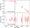 |
Fig. 11. Glitch detected with the algorithm on MJD 59732.9(1) in PSR J1048−5832 (glitch 11). Top: Residuals without considering the glitch. Bottom: Residuals after fitting for the glitch. |
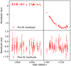 |
Fig. 12. Glitch detected with the algorithm on MJD 60090(10) in PSR J1048−5832 (glitch 12). Top: Residuals without considering the glitch. Bottom: Residuals after fitting for the glitch. |
We defined tg as halfway between the last pre-glitch and the first post-glitch observation. Both glitches are smaller in amplitude than those reported in Zubieta et al. (2023). The two glitches reported in Zubieta et al. (2023) correspond to glitches 9 and 10 in Liu et al. (2023). Those glitches, together with glitch eight reported in Liu et al. (2023), possess  . However, for these two new glitches (glitch 11 and glitch 12), we obtained
  , as reported for glitches 6 and 7 by Liu et al. (2023), which corresponds to a more typical behaviour for glitches.
In addition, while we were finishing this work, we detected a giant glitch in this pulsar (Table 2; Zubieta et al. (2024a)). A more thorough analysis of this glitch will be performed in future work, once we obtain a sufficient number of post-glitch TOAs from our ongoing monitoring program.
4.4. PSR J1644–4559 and PSR J1731–4744
We found 26 discrete events for PSR J1644−4559, 20 of which have Δν > 0, while for most of them the sign of  is unconstrained. The detections oscillate within small ranges of 4 × 10⁻¹⁰ < |Δν(s−1)| < 1.7 × 10⁻⁹ and
  . For PSR J1731−4744, the large uncertainties in its TOAs prevent us from performing a thorough search for small glitches, and we can see that the five detections are close to or below the detection limits.
4.5. PSR J1740–3015
We detected 11 events: 7 (63%) correspond to Δν < 0, while 3 show  . For the remaining event, the sign of
  is undefined. For the four events with Δν > 0, one possesses
  , one
, one  , while the sign of
  is undefined in the other two. The events are within the ranges of 2.1 × 10⁻⁹ < |Δν(s−1)| < 2.1 × 10⁻⁸ and
  .
.
The algorithm also detected the 2022 glitch (MJD 59935.1(4)) reported in Zubieta et al. (2023), which was excluded from Fig. 6. In this glitch, we detected a new long-scale decay term. We found τ = 124(2) d, with a degree of recovery of Q = 4.43(0.01)%, which can be seen in Fig. 13. We did not detect any change in  . Updated parameters for the glitch are shown in Table 2.
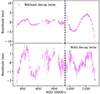 |
Fig. 13. Detection of a new decay term in the PSR J1740−3015 glitch on MJD = 59935.1(4). Top: Residuals without considering any decay term. Bottom: Residuals considering one decay term. |
5. Discussion
High-cadence pulsar observations are essential in order to characterise small glitches and short decay components in giant glitches (Espinoza et al. 2014; Basu et al. 2020; Singha et al. 2021; Zubieta et al. 2023), and to better understand the distinction between red noise and glitches. Considering that we detected one small glitch in PSR J1048−5832 and one in the Vela pulsar that were not detected by visual inspection of the residuals, this study highlights the importance of developing automated detection codes for systematically identifying glitches (Melatos et al. 2020; Singha et al. 2021). In addition, it is important to follow up each event with a more thorough analysis in order to classify them as glitches or timing irregularities, and in the former case also characterise the glitch parameters. It would be interesting to develop a more robust algorithm also capable of disentangling between small glitches and timing irregularities.
Such an approach is essential for accurately discerning the contribution of glitches to red noise and for distinguishing it from the inherent smooth wandering around a stable rotational model, enhancing our understanding of the mechanisms underlying red noise and glitches.
We identified irregularities in all six of the glitching pulsars studied, with different minimum and maximum sizes in |Δν| and  . In the particular case of the Vela pulsar, most of the events have a positive change in
  , that is, they are concentrated in quadrants I and II. Using a similar systematic search over more than 20 yr of data, Espinoza et al. (2021) found a comparable number of events in all quadrants, which is different from what we obtain. The only asymmetry these latter authors found was in the size distributions of the events in the second and fourth quadrants, which do not appear to come from the same parent distribution.
For the rest of the pulsars, events appear to be randomly distributed in the four quadrants. This resembles the result of Espinoza et al. (2021), demonstrating that the rotation of pulsars is affected by small variations in ν and  . Considering that only three of these events proved to be a glitch, we conclude that only a small portion of the timing noise seen in pulsars can be accounted for by small glitches. Therefore, our result indicates the presence of timing irregularities distinct from glitches, implying the existence of additional processes or phenomena that are not yet fully understood. A similar conclusion was reached by Cordes et al. (1988) and Espinoza et al. (2021) for the Vela pulsar. These small irregularities are sometimes presented as glitches or anti-glitches (se Tuo et al. 2024, and references therein), but we show that those irregularities are instead quite frequent, and show a relatively slow evolution compared to glitches, which are characterised by sudden significant changes in ν and
  that only take place sporadically.
Regarding the exploration of red noise phenomena, we discovered that, for PSR J0742−2822, the red noise diminishes significantly after the glitch event on MJD 59839.4(5), which was first detected by Grover et al. (2022). This behaviour resembles that reported by Keith et al. (2013) for the 2009 glitch in the same pulsar. Jones (1990) proposed that the red noise is influenced by the interaction between superfluid neutron vortices and the Coulomb lattice at the solid crust. In this scenario, there is a possible correlation between red noise and the presence of vortices that are pinned to the pulsar crust, with the red noise diminishing after vortices are dragged away during the glitch. Our results for J0742−2822 are also consistent with this interpretation.
In contrast, in the cases of PSR J1740−3015 and J0835−4510, we did not observe a significant decrease in red noise following the giant glitches on MJD 59935.1 and MJD 59417.6193, respectively. Considering that the properties of timing noise vary across the pulsar population (Shannon & Cordes 2010), and that the characteristic age of PSR J0742−2822 is ∼105 yr, whereas for PSR J0835−4510 and PSR J1740−3015 the characteristic age is a factor of about ten smaller (∼104 yr) (Manchester et al. 2005b), our result indicates that not only does the timing noise vary across the pulsar population but also the entanglement between red noise and glitches changes across the pulsar population. In addition, our result supports the theory that the red noise may come from both internal and external torque (Lyne et al. 2010; Melatos & Link 2014), and that the change in red noise behaviour during a glitch depends on the particular origin of red noise in each case. Another possibility is that this difference in red noise behaviour during a glitch could indicate the existence of different forms of turbulence in the superfluid interior of neutron stars (Melatos & Link 2014).
We also found a small glitch in the Vela pulsar reported in Table 2. This is 62 days after the 2021 giant glitch. Espinoza et al. (2021) and Dunn et al. (2023) reported one small glitch each in the Vela pulsar, 93 and 179 days after its giant glitch in 1991. Espinoza et al. (2021) reported another small glitch 134 days before the 2000 giant glitch. Lower et al. (2020) reported one small glitch 379 days after the 2013 giant glitch. In the case of the Vela pulsar, large glitches occur approximately every ∼3 years. However, the small glitches mentioned here do not seem to follow any pattern in their inter-glitch times. It is probable that many small glitches in the Vela pulsar have gone unnoticed due to the lack of permanent high-cadence monitoring. More detections of small glitches in frequently glitching pulsars are required to further investigate the underlying mechanisms and relationships between these events.
6. Conclusions
We present a detailed analysis of the IAR pulsar monitoring campaign between 2019 and 2023 and an algorithm to look for small glitches in timing data. Within the span of our data (of almost four years), we find three new small glitches, two in PSR J1048−5832, and one in the Vela pulsar, which were not detected by visual inspection. This demonstrates the necessity of developing algorithms to systematically search for small glitches, not only relying on visual inspection of residuals. Also, high-cadence monitoring is required to further study the population of small glitches in order to gain knowledge about glitches mechanisms.
In addition to the small glitches detected, we found many irregularities that could not be associated with glitches, which suggests the presence of a mechanism for red noise that is inherently different from the mechanisms that produce glitches. However, we show that for the 2022 glitch in PSR J0742−2822, the red noise diminished significantly after the glitch. Thus it cannot be assumed that red noise is a phenomenon that is completely independent from all glitches.
We note that additional observations after April 2024 have an improved bandwidth of 400 MHz, but these are not part of this legacy dataset.
Acknowledgments
FG and JAC are CONICET researchers and acknowledge support by PIP 0113 (CONICET). FG acknowledges support by PIBAA 1275 (CONICET). COL gratefully acknowledges the National Science Foundation (NSF) for financial support from Grant No. PHY-2207920. CME acknowledges support from the grant ANID FONDECYT 1211964. We also extend our gratitude to the technical staff at the IAR for their continuous efforts that enable our high-cadence observational campaign. JAC was also supported by grant PID2022-136828NB-C42 funded by the Spanish MCIN/AEI/ 10.13039/501100011033 and “ERDF A way of making Europe” and by Consejería de Economía, Innovación, Ciencia y Empleo of Junta de Andalucía as research group FQM-322.
References
- Antonelli, M., Basu, A., & Haskell, B. 2023, MNRAS, 520, 2813 [NASA ADS] [CrossRef] [Google Scholar]
- Antonopoulou, D., Haskell, B., & Espinoza, C. M. 2022, Rep. Prog. Phys., 85, 126901 [NASA ADS] [CrossRef] [Google Scholar]
- Araujo Furlan, S. B., Zubieta, E., Gancio, G., et al. 2024, Rev. Mex. Astron. Astrofis. Conf. Ser., 56, 85 [NASA ADS] [Google Scholar]
- Arzoumanian, Z., Nice, D. J., Taylor, J. H., & Thorsett, S. E. 1994, ApJ, 422, 671 [NASA ADS] [CrossRef] [Google Scholar]
- Basu, A., Joshi, B. C., Krishnakumar, M. A., et al. 2020, MNRAS, 491, 3182 [NASA ADS] [Google Scholar]
- Basu, A., Shaw, B., Antonopoulou, D., et al. 2022, MNRAS, 510, 4049 [NASA ADS] [CrossRef] [Google Scholar]
- Baym, G., Pethick, C., & Pines, D. 1969, Nature, 224, 673 [NASA ADS] [CrossRef] [Google Scholar]
- Cordes, J. M., Downs, G. S., & Krause-Polstorff, J. 1988, ApJ, 330, 847 [NASA ADS] [CrossRef] [Google Scholar]
- Dunn, L., Melatos, A., Espinoza, C. M., Antonopoulou, D., & Dodson, R. 2023, MNRAS, 522, 5469 [NASA ADS] [CrossRef] [Google Scholar]
- Espinoza, C. M., Lyne, A. G., Stappers, B. W., & Kramer, M. 2011, MNRAS, 414, 1679 [NASA ADS] [CrossRef] [Google Scholar]
- Espinoza, C. M., Antonopoulou, D., Stappers, B. W., Watts, A., & Lyne, A. G. 2014, MNRAS, 440, 2755 [NASA ADS] [CrossRef] [Google Scholar]
- Espinoza, C. M., Antonopoulou, D., Dodson, R., Stepanova, M., & Scherer, A. 2021, A&A, 647, A25 [Google Scholar]
- Fuentes, J. R., Espinoza, C. M., Reisenegger, A., et al. 2017, A&A, 608, A131 [NASA ADS] [CrossRef] [EDP Sciences] [Google Scholar]
- Gancio, G., Lousto, C. O., Combi, L., et al. 2020, A&A, 633, A84 [NASA ADS] [CrossRef] [EDP Sciences] [Google Scholar]
- Grover, H., Singha, J., Joshi, B. C., & Arumugam, P. 2022, ATel., 15629 [Google Scholar]
- Grover, H., Joshi, B. C., Singha, J., et al. 2024, ArXiv e-prints [arXiv:2405.14351] [Google Scholar]
- Gügercinoğlu, E., Ge, M. Y., Yuan, J. P., & Zhou, S. Q. 2022, MNRAS, 511, 425 [CrossRef] [Google Scholar]
- Haskell, B., & Melatos, A. 2015, Int. J. Mod. Phys. D, 24, 1530008 [NASA ADS] [CrossRef] [Google Scholar]
- Hobbs, G. B., Edwards, R. T., & Manchester, R. N. 2006, MNRAS, 369, 655 [Google Scholar]
- Hobbs, G., Lyne, A. G., & Kramer, M. 2010, MNRAS, 402, 1027 [NASA ADS] [CrossRef] [Google Scholar]
- Hobbs, G., Coles, W., Manchester, R. N., et al. 2012, MNRAS, 427, 2780 [NASA ADS] [CrossRef] [Google Scholar]
- Hotan, A. W., van Straten, W., & Manchester, R. N. 2004, PASA, 21, 302 [Google Scholar]
- Janssen, G. H., & Stappers, B. W. 2006, A&A, 457, 611 [NASA ADS] [CrossRef] [EDP Sciences] [Google Scholar]
- Jones, P. B. 1990, MNRAS, 246, 364 [NASA ADS] [Google Scholar]
- Keith, M. J., Shannon, R. M., & Johnston, S. 2013, MNRAS, 432, 3080 [NASA ADS] [CrossRef] [Google Scholar]
- Lentati, L., Alexander, P., Hobson, M. P., et al. 2014, MNRAS, 437, 3004 [NASA ADS] [CrossRef] [Google Scholar]
- Liu, P., Yuan, J. P., Ge, M. Y., et al. 2023, ArXiv e-prints [arXiv:2312.04305] [Google Scholar]
- Lopez Armengol, F. G., Lousto, C. O., del Palacio, S., et al. 2019, ATel., 12482 [Google Scholar]
- Lorimer, D. R., & Kramer, M. 2004, Handbook of Pulsar Astronomy, 4 [Google Scholar]
- Lousto, C. O., Missel, R., Prajapati, H., et al. 2022, MNRAS, 509, 5790 [Google Scholar]
- Lousto, C. O., Missel, R., Zubieta, E., et al. 2024, Rev. Mex. Astron. Astrofis. Conf. Ser., 56, 134 [NASA ADS] [Google Scholar]
- Lower, M. E., Bailes, M., Shannon, R. M., et al. 2020, MNRAS, 494, 228 [CrossRef] [Google Scholar]
- Luo, J., Ransom, S., Demorest, P., et al. 2021, ApJ, 911, 45 [NASA ADS] [CrossRef] [Google Scholar]
- Luo, J., Ransom, S., Demorest, P., et al. 2019, Astrophysics Source Code Library [record ascl:1902.007] [Google Scholar]
- Lyne, A., Hobbs, G., Kramer, M., Stairs, I., & Stappers, B. 2010, Science, 329, 408 [NASA ADS] [CrossRef] [Google Scholar]
- Manchester, R. N. 2018, Pulsar Astrophysics the Next Fifty Years, eds. P. Weltevrede, B. B. P. Perera, L. L. Preston, & S. Sanidas, 337, 197 [Google Scholar]
- Manchester, R. N., Hobbs, G. B., Teoh, A., & Hobbs, M. 2005a, AJ, 129, 1993 [Google Scholar]
- Manchester, R. N., Hobbs, G. B., Teoh, A., & Hobbs, M. 2005b, VizieR Online Data Catalog: VII/245 [Google Scholar]
- Melatos, A., & Link, B. 2014, MNRAS, 437, 21 [NASA ADS] [CrossRef] [Google Scholar]
- Melatos, A., & Warszawski, L. 2009, ApJ, 700, 1524 [NASA ADS] [CrossRef] [Google Scholar]
- Melatos, A., Dunn, L. M., Suvorova, S., Moran, W., & Evans, R. J. 2020, ApJ, 896, 78 [NASA ADS] [CrossRef] [Google Scholar]
- Parthasarathy, A., Shannon, R. M., Johnston, S., et al. 2019, MNRAS, 489, 3810 [Google Scholar]
- Ransom, S. 2011, Astrophysics Source Code Library [record ascl:1107.017] [Google Scholar]
- Ransom, S. M., Cordes, J. M., & Eikenberry, S. S. 2003, ApJ, 589, 911 [NASA ADS] [CrossRef] [Google Scholar]
- Shannon, R. M., & Cordes, J. M. 2010, ApJ, 725, 1607 [NASA ADS] [CrossRef] [Google Scholar]
- Shannon, R. M., Lentati, L. T., Kerr, M., et al. 2016, MNRAS, 459, 3104 [NASA ADS] [CrossRef] [Google Scholar]
- Shaw, B., Mickaliger, M. B., Stappers, B. W., et al. 2022, ATel., 15622 [Google Scholar]
- Singha, J., Basu, A., Krishnakumar, M. A., Joshi, B. C., & Arumugam, P. 2021, MNRAS, 505, 5488 [NASA ADS] [CrossRef] [Google Scholar]
- Sosa Fiscella, V., del Palacio, S., Combi, L., et al. 2021a, ApJ, 908, 158 [Google Scholar]
- Sosa-Fiscella, V., Zubieta, E., del Palacio, S., et al. 2021b, ATel., 14806 [Google Scholar]
- Taylor, J. H. 1992, Philos. Trans. R. Soc. London Ser. A, 341, 117 [NASA ADS] [CrossRef] [Google Scholar]
- Tuo, Y., Serim, M. M., Antonelli, M., et al. 2024, ApJ, 967, L13 [NASA ADS] [CrossRef] [Google Scholar]
- Yu, M., Manchester, R. N., Hobbs, G., et al. 2013, MNRAS, 429, 688 [NASA ADS] [CrossRef] [Google Scholar]
- Zhou, S., Gügercinoğlu, E., Yuan, J., Ge, M., & Yu, C. 2022a, Universe, 8, 641 [NASA ADS] [CrossRef] [Google Scholar]
- Zhou, Z.-R., Wang, J.-B., Wang, N., et al. 2022b, Res. Astron. Astrophys., 22, 095008 [CrossRef] [Google Scholar]
- Zubieta, E., Del Palacio, S., Garcia, F., et al. 2022a, ATel., 15638 [Google Scholar]
- Zubieta, E., Furlan, S. B. A., Palacio, S. D., et al. 2022b, ATel., 15838 [Google Scholar]
- Zubieta, E., Missel, R., Sosa Fiscella, V., et al. 2023, MNRAS, 521, 4504 [Google Scholar]
- Zubieta, E., Araujo Furlan, S. B., del Palacio, S., et al. 2024a, ATel., 16580 [Google Scholar]
- Zubieta, E., del Palacio, S., García, F., et al. 2024b, Rev. Mex. Astron. Astrofis. Conf. Ser., 56, 161 [NASA ADS] [Google Scholar]
All Tables
Updated parameters for all glitches detected by PuMA collaboration between MJD 58832 and MJD 60411.
All Figures
|
Fig. 1. Residuals for pulsars that did not have a giant glitch during our campaign. |
| In the text | |
|
Fig. 2. Residuals for pulsars that experienced a giant glitch during our campaign. |
| In the text | |
|
Fig. 3. Process to adjust the TOA uncertainties. Top: We keep a short data span with flat residuals. Bottom: We add the parameters EFAC and EQUAD (Eq. 3) calculated with TempoNest. |
| In the text | |
|
Fig. 4. Signature of a glitch with Δν > 0 and |
| In the text | |
|
Fig. 5. Schematic representation of steps 1 and 2 of the algorithm described in Sect. 3.2. Example with Nmin = 5. Top: ν and |
| In the text | |
|
Fig. 6. Irregularities detected by our algorithm in the six pulsars. The colour bar indicates the significance of the detection. The two shaded regions correspond to detection limits following Eq. 4, calculated with σTOA and σTOA + ΔσTOA, respectively. |
| In the text | |
|
Fig. 7. Detection of a new decay term in the PSR J0742−2822 glitch on MJD 59839.4(5). Top: Residuals without considering any decay term. Bottom: Residuals considering one decay term of 33.4(5) d. |
| In the text | |
|
Fig. 8. Timing parameters of J0742−2822 calculated in 100 d windows with consecutive windows overlapping by 50 TOAs; the time window is represented with a horizontal error bar. Top: Evolution of |
| In the text | |
|
Fig. 9. Detection of a new decay term in the 2021 Vela glitch. Top: Residuals without considering long decay term. Bottom: Residuals considering the long decay term of 535(8) d. We note the much smaller residual scale. The signal that remains is the timing noise of the Vela pulsar. |
| In the text | |
|
Fig. 10. Detection of a small glitch 62 days after the 2021 giant glitch. Top: Residuals without considering the small glitch. Bottom: Residuals after fitting for the small glitch. |
| In the text | |
|
Fig. 11. Glitch detected with the algorithm on MJD 59732.9(1) in PSR J1048−5832 (glitch 11). Top: Residuals without considering the glitch. Bottom: Residuals after fitting for the glitch. |
| In the text | |
|
Fig. 12. Glitch detected with the algorithm on MJD 60090(10) in PSR J1048−5832 (glitch 12). Top: Residuals without considering the glitch. Bottom: Residuals after fitting for the glitch. |
| In the text | |
|
Fig. 13. Detection of a new decay term in the PSR J1740−3015 glitch on MJD = 59935.1(4). Top: Residuals without considering any decay term. Bottom: Residuals considering one decay term. |
| In the text | |
Current usage metrics show cumulative count of Article Views (full-text article views including HTML views, PDF and ePub downloads, according to the available data) and Abstracts Views on Vision4Press platform.
Data correspond to usage on the plateform after 2015. The current usage metrics is available 48-96 hours after online publication and is updated daily on week days.
Initial download of the metrics may take a while.