| Issue |
A&A
Volume 628, August 2019
|
|
|---|---|---|
| Article Number | A47 | |
| Number of page(s) | 12 | |
| Section | The Sun | |
| DOI | https://doi.org/10.1051/0004-6361/201935510 | |
| Published online | 06 August 2019 | |
The diagnostic potential of the weak field approximation for investigating the quiet Sun magnetism: the Si I 10 827 Å line
1
Main Astronomical Observatory, National Academy of Sciences, 27 Zabolotnogo Street, Kyiv 03143, Ukraine
e-mail: This email address is being protected from spambots. You need JavaScript enabled to view it.
2
Astronomical Observatory, Kyiv Shevchenko National University, 3 Observatorna Street, Kyiv 04053, Ukraine
3
Astronomical Observatory, Lviv Ivan Franko National University, 8 Kyryla i Mefodiya Street, Lviv 79005, Ukraine
4
Instituto de Astrofísica de Canarias, 38205 La Laguna, Tenerife, Spain
e-mail: This email address is being protected from spambots. You need JavaScript enabled to view it.
, This email address is being protected from spambots. You need JavaScript enabled to view it.
5
Universidad de La Laguna, Departamento de Astrofísica, 38206 La Laguna, Tenerife, Spain
6
Consejo Superior de Investigaciones Científicas, Spain
Received:
21
March
2019
Accepted:
10
June
2019
Abstract
Aims. We aim to investigate the validity of the weak field approximation (WFA) for determining magnetic fields in quiet regions of the solar photosphere using the polarization caused by the Zeeman effect in the Si I 10 827 Å line.
Methods. We solved the NLTE line formation problem by means of multilevel radiative transfer calculations in a three-dimensional (3D) snapshot model taken from a state-of-the-art magneto-convection simulation of the small-scale magnetic activity in the quiet solar photosphere. The 3D model used is characterized by a surface mean magnetic field strength of about 170 G. The calculated Stokes profiles were degraded because of the atmospheric turbulence of Earth and light diffraction by the telescope aperture. We apply the WFA to the Stokes I, Q, U, V profiles calculated for different seeing conditions and for the apertures of the VTT, GREGOR, EST and DKIST telescopes. We compare the inferred longitudinal and transverse components of the magnetic field with the original vertical and horizontal fields of the 3D model.
Results. We find that with a spatial resolution significantly better than 0.5″ the surface maps of the magnetic field inferred from the Stokes profiles of the Si I 10 827 Å line applying the WFA are close to the magnetic field of the model on the corrugated surface, corresponding to line optical depth unity at Δλ ≈ 0.1 Å for a disk-center line of sight. The correlation between them is relatively high, except that the inferred longitudinal and transverse components of the magnetic field turn out to be lower than in the 3D model.
Conclusions. The use of the WFA for interpreting high-spatial-resolution spectropolarimetric observations of the Si I 10 827 Å line obtained with telescopes like GREGOR, EST, and DKIST allows the longitudinal and transverse components of the magnetic field to be retrieved with reasonable precision over the whole quiet solar photosphere, the result being worse for telescopes of lower aperture.
Key words: Sun: magnetic fields / Sun: photosphere / line: formation / radiative transfer
© ESO 2019
1. Introduction
The polarization of the Si I 10 827 Å line is an important observable for studying solar magnetic fields. Due to its location in the near-infrared (NIR) spectral region, the polarization signals induced by the Zeeman effect in this line are more sensitive to the presence of a magnetic field than other lines in the optical part of the solar spectrum with similar (geff = 1.5) or even larger effective Landé factors. The line formation region of the Si I 10 827 Å line (Shchukina et al. 2017; Sukhorukov 2012) covers a large portion of the photosphere, from the bottom of the photosphere to near the temperature minimum. Moreover, there are several other advantages compared to observations at shorter wavelengths: for example, better atmospheric seeing, less atmospheric and instrumental scattering, and smaller instrumental polarization (see, e.g., Penn 2014). As a result, the Si I 10 827 Å line appears to represent a good opportunity to “trace” magnetic fields throughout the whole solar photosphere.
There have been many spectropolarimetric investigations of solar magnetic fields using the Si I 10 827 Å line. For example, Rüedi et al. (1995) interpreted observed Stokes I and V profiles of this line by carrying out local thermodynamic equilibrium (LTE) radiative transfer calculations through a two-component model atmosphere composed of a nonmagnetic part and a magnetic one. Later, various LTE inversion codes like SIR (Ruiz Cobo & del Toro Iniesta 1992), SPINOR (Frutiger et al. 2000), and Milne-Eddington (e.g., Borrero et al. 2014) were applied to the Stokes profiles of the Si I 10 827 Å line to study magnetic fields in active regions (Solanki et al. 2003; Lagg et al. 2004; Wiegelmann et al. 2005), active region filaments (Kuckein et al. 2012; Xu et al. 2012; Yelles Chaouche et al. 2012), pre-flare, flare, and post-flare stages (Kuckein et al. 2015), a sunspot light bridge (Felipe et al. 2016), a sunspot penumbra (Joshi et al. 2016), and an arch filament system in a sunspot group (Balthasar et al. 2018). Recently, Orozco Suárez et al. (2017) inferred the magnetic field vector stratification in the umbra atmosphere of a sunspot applying the NICOLE inversion code (Socas-Navarro et al. 2015), accounting for non-local thermodynamic equilibrium (NLTE) effects in the Si I 10827 Å line.
The development of new telescopes and IR spectropolarimeters provide new opportunities to retrieve magnetic fields from high-resolution observations of this line. The most important examples are the 4 m Daniel K. Inouye Solar Telescope (DKIST, Keil et al. 2011) and the 4 m European Solar Telescope (EST, Collados et al. 2013; Matthews et al. 2016) with planned IR instruments. At present, many studies are using the 1.5 m GREGOR solar telescope (Denker et al. 2012; Soltau et al. 2012; Felipe et al. 2016; Joshi et al. 2016; Balthasar et al. 2018) with the GREGOR Infrared Spectrograph (GRIS, Collados et al. 2012).
These ground-based facilities for solar IR spectropolarimetric observations requires further development and improvement in the diagnostic tools. Nowadays, a large number of methods based on the Zeeman effect are widely employed by the solar physics community to determine quantitative properties of the magnetic fields. Among them are various inversion codes, spectral line synthesis in 3D magnetohydrodynamic (MHD) models and comparison with observations, techniques based on exploiting the hyperfine structure of some atoms, as well as simplified approaches like the line ratio method, the weak field approximation (WFA), the bisector, and the center-to-gravity techniques (see, e.g., Solanki 1993; Landi Degl’Innocenti & Landolfi 2004; Khomenko 2006; Shchukina & Trujillo Bueno 2013; del Toro & Ruiz Cobo 2006, and references therein).
Such diagnostic tools, applied to different spectral lines (mainly to Fe I lines in the visible and NIR range) make it possible to study the magnetic field properties both of active and quiet regions of the Sun. The inference of the magnetic field properties of the quiet areas using the Si I 10 827 Å line are always challenged by the weakness of the Zeeman polarization signals (especially in Stokes Q and U) compared to those observed in the active regions. In addition, in the quiet regions, the impact of deviations from LTE (i.e., NLTE), both on the intensity and on the linearly and circularly polarized profiles of the Si I 10 827 Å line, turns out to be significant. The difference between the NLTE and LTE intensity profiles of this line varies considerably across the solar surface, with a well-pronounced dependence on the line depth (Bard & Carlsson 2008; Sukhorukov & Shchukina 2012; Sukhorukov 2012; Shchukina et al. 2012, 2017). The Stokes Q, U, V profile changes caused by deviation from LTE are comparable to the values of the Stokes amplitudes themselves. For the Stokes V parameter, there is a clear correlation between the magnitude of the NLTE effects and magnetic field strength (Shchukina et al. 2017). Up to now, there have been no attempts to apply any NLTE inversion code to the Si I 10 827 Å line in order to infer the magnetic properties of the quiet solar atmosphere.
In this paper we rely on a more simple approach. We focus on the WFA to evaluate the extent to which the magnetic fields of the quiet Sun inferred from the Si I 10 827 Å line using this approximation are close to the real solar values. Ground-based observations are affected by the atmospheric turbulence of the Earth (seeing) and instrumental effects due to light diffraction by the limited telescope aperture (the finite spatial resolution of the telescope), in addition to finite instrumental width of the filters used, stray light, and so on. In this paper we tackle the problem of studying degradation effects caused by seeing and by the diffraction limit of the telescope. We also discuss the effects of photon noise on the circular and linear polarization signals.
The paper is organized as follows. Section 2 describes the 3D snapshot model atmosphere employed in this study, the methods and the atomic data used for the spectral synthesis of the Stokes I, Q, U, V profiles of the Si I 10 827 Å line, and the procedure of spatial smearing of such profiles. In Sect. 3 we give the expressions for the Stokes parameters in the weak field limit and discuss the conditions needed to hold it in the solar quiet atmosphere. Section 4 presents results for the longitudinal and transverse components of the magnetic field inferred using the weak field approximation. Finally, Sect. 5 summarizes our main conclusions.
2. Input data and method
2.1. Model atmosphere
The topic of our study is the quiet regions of the solar disk. We used the most magnetized 3D model from the magneto-convection simulations with small-scale dynamo action performed by Rempel (2014). The chosen 3D snapshot model, which has a surface mean field strength of about 170 G, represents the small-scale magnetic activity of the quiet photosphere relatively accurately (see del Pino Alemán et al. 2018, and more references therein). The vertical unsigned flux density of the model ⟨|BZ|⟩ ≃ 80 G in the visible surface layers and the net magnetic flux is zero. This model was interpolated to a coarser grid of 77 × 77 × 102 points with the aim of facilitating the NLTE radiative transfer calculations. It corresponds to resolutions of 80 km in the horizontal directions and 8 km in the vertical direction. Taking into account the fact that the line formation region of the Si I 10 827 Å line covers a large portion of the photosphere, we used the uppermost ∼0.8 Mm layer for our radiative transfer calculations. A more detailed description of the snapshot model employed and its comparison with other 3D MHD models can be found in Shchukina & Trujillo Bueno (2015) and Shchukina et al. (2017).
2.2. Synthesis of Stokes profiles
We solved the NLTE radiative transfer problem of the Si I 10 827 Å line in the 3D MHD model atmosphere of Rempel (2014) mentioned above, neglecting the effects of horizontal radiative transfer (i.e., we used the so-called 1.5D approximation).
We obtained the self-consistent solution of the statistical and radiative transfer equations applying an efficient multilevel transfer code developed by Shchukina & Trujillo Bueno (2001). To this end, we used a relatively simple silicon model atom which is suitable for an accurate description of the physics of the Si I 10 827 Å line formation (see Shchukina et al. 2017). The model contains sixteen levels connected by six radiative bound-bound and fifteen bound-free radiative transitions. Further details of the model and atomic data, including the oscillator strengths, bound-free cross-sections, collision rates, and so on, are described in Shchukina et al. (2017).
We used the field-free population departure coefficients of the lower and upper levels of the Si I 10 827 Å line, obtained from the self-consistent solution of the statistical and radiative transfer equations, as input for the Stokes-vector formal solver. We define the departure coefficients as the ratio of the NLTE atomic level populations to the LTE ones.
We calculated the emergent Stokes profiles of the Si I 10 827 Å line at the solar disk center applying a radiative-transfer code based on the DELOPAR method proposed by Trujillo Bueno (2003). We solved the Zeeman line transfer problem neglecting atomic level polarization (see Trujillo Bueno & Landi Degl’Innocenti 1996, and more references therein).
The Stokes profiles of the Si I 10 827 Å line were synthesized for every (x, y) vertical column of the 3D MHD snapshot with a spectral resolution 10 mÅ from −3 Å to +3 Å around the central line wavelength. We used the solar silicon abundance ASi = 7.55 recommended by Grevesse & Sauval (1998). This value agrees with the silicon abundance obtained by Shchukina et al. (2012) through NLTE spectral synthesis in a 3D hydrodynamical model of the solar photosphere. We normalized the Stokes profiles to the mean continuum intensity ⟨Ic⟩ obtained by averaging over the horizontal direction of the snapshot. The continuum intensity was calculated using our background continuum opacity code (see Shchukina & Trujillo Bueno 2001, 2015, and more references therein). More detailed information on the NLTE spectral synthesis of the Si I 10 827 Å line can be found in Shchukina et al. (2017). Here it suffices to reiterate that for this line the main NLTE effect is the line source function deficit as compared with the LTE predictions.
We estimated the formation heights of the the Si I 10 827 Å line in the 3D MHD model atmosphere of Rempel (2014) using the concept of “Eddington-Barbier height of line formation”. Therefore, at each (x, y)-point, we calculated the height HΔλ and the corresponding continuum optical depth τ5(Δλ) at 5000 Å, where the line optical depth τΔλ is equal to unity. Mean values of ⟨H⟩ and ⟨τ5⟩ for each line wavelength Δλ were computed by averaging the corresponding quantities along the horizontal directions. Figure 1 shows histograms of the NLTE heights of formation of the Si I 10 827 Å line determined for the line continuum and for three wavelength points. We can see that the formation heights HΔλ of this line fluctuate significantly across the surface of the 3D model snapshot. The line-formation region covers a large portion of the photosphere, from the bottom of the photosphere (the continuum) to the middle (the line wings where the Stokes V peaks are located) and up to near the temperature minimum (the line center). The NLTE shifts in the formation height of the Si I 10 827 Å line are less than a few tens of kilometers throughout the surface of the 3D snapshot model (see Shchukina et al. 2017).
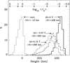 |
Fig. 1. Histograms of the NLTE heights of formation calculated at four wavelengths within the Si I 10 827 Å line intensity profile. The top horizontal axis gives the mean optical depths ⟨τ5⟩ corresponding to the heights shown in the bottom horizontal axis. The mean heights of formation and wavelengths are shown close to each of the histograms. The histograms were calculated using the 3D snapshot model with ⟨|BZ|⟩ = 80 G (Rempel 2014) and the Si I model with six bound-bound transitions described by Shchukina et al. (2017). |
2.3. Spatial smearing
The Stokes profiles of the Si I 10 827 Å line synthesized in the 3D snapshot model represent “unsmeared (perfect) observations”. The spatial resolution of these numerical data, that is, the grid resolution, is 80 km. Here we consider two effects that degrade the original Stokes profiles: the finite spatial resolution determined by the telescope aperture and the effects of smearing caused by the turbulence of the atmosphere of the Earth (seeing). In order to mimic the effects caused by the telescope and seeing we follow the procedure described in Shchukina et al. (2009). At each line wavelength, the original 2D Stokes I, Q, U, and V maps were Fourier-transformed and multiplied by the modulation transfer function (MTF) taken from Fried (1966). An inverse Fourier transform gives us the images registered by detector, that is, the “observed” images, affected by the finite spatial resolution of the telescope and seeing effects. Only three parameters define the resulting image quality: the observed wavelength λ, the diameter D of the telescope, and the Fried parameter R0 (Fried 1966; Korff 1973). The Fried parameter depends on the seeing conditions and describes the characteristic size of the atmospheric turbulence cells at a given wavelength. In our study we simulate “real observations” for a set of R0 values at λ = 10 827 Å using the diameters of the VTT, GREGOR, and EST (DKIST) telescopes.
We determine the Fried parameter R0 from observed rms continuum contrast δIrms of the solar granulation. To this end, we set up theoretical calibration curves. We calculated them by means of the radiative transfer formal solution for the solar continuum intensity in the same 3D snapshot model of Rempel (2014) used for the synthesis of the Si I 10 827 Å Stokes profiles. The theoretical dependences of the δIrms contrast on the Fried parameter R0 for three values of the telescope diameter using this approach are shown in Fig. 2. According to this figure the rms continuum contrast δIrms for observations with the original spatial resolution (no smearing due to effects of the telescope aperture and seeing) at the wavelength of the Si I 10 827 Å line is 7.55%. For observations with a spatial resolution corresponding to the diffraction limit of the assumed telescope this contrast is smaller. It changes from 5.19% to 7.02% as the telescope diameter increases from D = 0.7 m (VTT) to D = 4.0 m (EST).
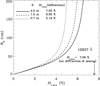 |
Fig. 2. Root-mean-square continuum contrast δIrms as a function of the Fried parameter R0 at wavelength λ = 10827 Å. Dotted, dashed, and solid curves correspond to the telescope diameters 0.7, 1.5, and 4 m, respectively. The δIrms contrast for observations affected only by the diffraction limit of the VTT(D = 0.7 m), GREGOR (D = 1.5 m) and EST/DKIST (D = 4.0 m) telescopes (no seeing effects) are indicated in the upper part of this figure. The vertical arrow in the lower right corner marks the δIrms value for the “perfect” observations corresponding to the case of the original spatial resolution (no smearing caused by the telescope and seeing effects). The calibration curves for the determination of the Fried parameter R0 were calculated using the radiative transfer formal solution for the continuum intensity in the chosen 3D snapshot model of Rempel (2014). |
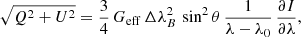
3. The weak field approximation
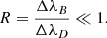
The WFA makes it possible to determine the magnetic field without solving the Stokes-vector transfer equations (see full details in Landi Degl’Innocenti & Landolfi 2004); this requires that the field be weak. In other words, the Zeeman splitting has to be significantly smaller than the Doppler width of the line:

with ΔλD being the Doppler width of the line given by

ΔλB the Zeeman splitting of the line given by

with ωT being the thermal velocity, B the magnetic field strength, λ0 the wavelength of the line, c the speed of light, and geff the effective Landé factor. For the Si I 10 827 Å line geff = 1.5.
In the 3D model of Rempel (2014), at the formation heights of the Si I 10 827 Å line wings and the line core (−0.25 ≤ Δλ ≤ 0.25 Å) more than 90% of the grid points have magnetic field strengths B weaker than 300 G and the thermal velocity ωT is in the range between 1 km s−1 and 2 km s−1. For these grid-points we find
which indicates that in the 3D Rempel model the Si I 10 827 Å line is close to the weak field regime.
In this case, the longitudinal component of the magnetic field BL = B cos θ can be estimated using the following expression for the circular polarization (Landi Degl’Innocenti & Landolfi 2004):
 (1)
(1)
where  is the spectral derivative of the intensity and θ is the angle between the magnetic field and the line-of-sight. This equation is strictly satisfied when the field BL is constant in the line formation region.
The transverse component of the magnetic field BT = B sin θ in the weak field limit can be found using the Stokes Q and U parameters as follows (see Landi Degl’Innocenti & Landolfi 2004)
 (2)
(2)
where  is the total linear polarization P and Geff is the second-order effective Landé factor which for the Si I 10 827 Å line is equal to 2.25. Equation (2) is valid for the line wings provided that the azimuth γ of the magnetic field, the magnetic intensity BT, and the thermal velocity ωT do not change in the layers where the Stokes Q and U signals originate. In the quiet solar photosphere the above-mentioned requirement of the weak field approximation for the magnetic field and other physical quantities in the formation region of the Stokes parameters of the Si I 10 827 Å line is not satisfied. Here we indicate two facts that support this statement. Firstly, there are strongly asymmetric and irregular shapes of the Stokes profiles for different spectral lines observed in the solar inter-network, which are found also in the 3D MHD simulations (e.g., Illing et al. 1975; Khomenko et al. 2003, 2005; Martínez González et al. 2016; Shchukina et al. 2017). Figure 3 shows that this is also true for the Si I 10 827 Å line formed in the 3D magneto-convection model of Rempel (2014). Such a complicated shape of the Stokes profiles is first of all caused by the changes of the magnetic field along the line-of-sight in the presence of velocity gradients (e.g., Khomenko 2006, and references therein). Secondly, in the model of Rempel (2014) the shape of
 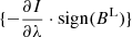 and of the V profiles of the Si I 10 827 Å line turns out to be different (see Fig. 3). We note that in the weak field approximation of Eq. (1), these profiles should be proportional to each other (Stenflo et al. 1984).
 |
Fig. 3. Left, from top to bottom: disk-center profiles of the intensity I, intensity derivative |

In order to clarify this issue, we determined the wavelength positions Δλ of the Stokes V and  profile peaks for all (x, y)-grid points of the snapshot. We identify the peaks with the maximum absolute values of these profiles. A histogram of the Δλ positions shown in Fig. 4 demonstrates that the median values of the wavelength positions of the Stokes V blue and red lobe peaks of the Si I 10 827 Å line are slightly different (−0.08 Å and 0.1 Å, respectively) and do not coincide with those of the
  profile peaks. On average, the latter are located around ±0.07 Å. Figure 4 also demonstrates that there is a sufficiently large number of Stokes V profiles with peaks located at Δλ ≥ 0.15 Å, while the number of the intensity derivative profiles with peaks at these wavelengths is noticeably smaller. Interestingly, in contrast to the peak wavelength positions the zero-crossing positions of the Stokes V profiles and the intensity derivative are close to each other (see Fig. 5). We note that we determined these positions in the range λ0 ± 0.05 Å, where λ0 are the wavelength positions of the Stokes I profile minima.
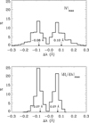 |
Fig. 4. Top: histogram of wavelength positions of the unsigned Stokes |V| peaks of the Si I 10 827 Å line formed in the 3D snapshot model of Rempel (2014). Bottom: same but the for the unsigned intensity derivative |

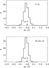 |
Fig. 5. Top: histogram of the zero-crossing wavelength positions of the Stokes V profiles of the Si I 10 827 Å line formed in the 3D snapshot model. Bottom: same but for the intensity derivative. Arrows and numbers indicate the mean values of such zero-crossing positions. |
Finally, we conclude that for most (x, y)-grid surface points of the 3D snapshot model the requirement of the constant field in the formation region of the Si I 10 827 Å line does not hold. To what extent the failure of this condition will affect the results obtained using the weak field approximation is one of the main issues considered in the following section.
4. Results
4.1. Stokes signals with original and reduced spatial resolution
Figure 6 displays 2D maps of the intensity derivative  , the total linear polarization
  , and the circular polarization V in the blue wing of the Si I 10 827 Å line calculated at the solar disk center of the model. We note that these values are measured in units of the mean continuum intensity ⟨Ic⟩ at the wavelengths where the modulus of the intensity derivative is maximum. The top panels of this figure show the spatial variations of the original Stokes signals calculated in the 3D snapshot which mimic “unsmeared observations”. The impact of the diffraction limit of the EST/DKIST-like telescopes (D = 4 m) is shown in the middle panels. The bottom panels show the surface variations of the Stokes signals affected by the finite spatial resolution of this telescope and seeing effects. We quantified the latter using R0 = 50 cm as the typical Fried parameter value for NIR observations (see Felipe et al. 2016; Joshi et al. 2016; Martínez González et al. 2016; Orozco Suárez et al. 2017). It corresponds to ∼0.54″ of spatial resolution at the 10 827 Å wavelength.
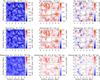 |
Fig. 6. From left to right: maps of the intensity derivative |

Figure 6 shows that the Stokes P and V signals in the Si I 10 827 Å line are usually larger in the intergranuler lanes. Typically, the P signals are small while the Stokes V signals have significantly larger amplitudes. The latter is easy to understand bearing in mind that for sufficiently “weak” photospheric magnetic fields, such as in the 3D MHD snapshot model of Rempel (2014), the circular polarization signal scales with the ratio
 (3)
(3)
On the contrary, the linear polarization signals are approximately proportional to R2.
Our Stokes parameters calculations of the Si I 10 827 Å line in the 3D MHD snapshot model reveal that the number of pixels where the total linear polarization P/⟨Ic⟩≥0.03% for the unsmeared case is ∼60%. For Stokes V this value is 89%. Interestingly, while only 0.6% of the pixels show linear polarization signals above 1%, the number of pixels with circular polarization above this value is considerably larger (i.e., ≈15%). We note that the limiting signal of 0.03% is nothing but the 3σ level, where σ is the noise level in the spectro-polarimetric observations obtained by Martínez González et al. (2016) using GRIS in combination with the Tenerife Infrared Polarimeter (Collados et al. 2012). The spatial resolution corresponding to the diffraction limit of an EST/DKIST-like telescope reduces the number of pixels with Stokes signals above 0.03% only slightly on average, by ≈1%. The impact of the combined telescope and seeing effects turn out to be more important. Now, ∼50% of the pixels have linear polarization signal above 0.03%. For the Stokes V signal these effects are less pronounced. In the latter case the number of pixels where V/⟨Ic⟩≥0.03% decreases by no more than ∼3%.
The strongest effect produced by spatial smearing is a reduction of the  , P, and V peaks. Figure 6 allows us to estimate the degree of such a deterioration. Each panel of Fig. 6 indicates the minimum and maximum values of the intensity derivative
  , and of Stokes P and V measured at the wavelengths of the intensity derivative peaks. As we can see, with deterioration in resolution, the maximum value of the Stokes V signal in the Si I 10 827 Å line quickly decreases from 17% for “unsmeared observations” to 2% for a spatial resolution of 0.54″.
The maximum total linear polarization, being small by itself, turns out to be even smaller, decreasing from 2.22% for the unsmeared case to 0.28% for EST/DKIST-like observations affected by seeing. We note that observations with a 4 m telescope outside the atmosphere of Earth would make it possible to obtain P and V signals that are relatively close to the “unsmeared” ones. Figure 6 also shows that unlike P and V, the intensity derivative peaks of the Si I 10 827 Å line are much less sensitive to spatial smearing; the maximum value of its modulus decreases from ∼1.2% to ∼0.5%.
4.2. Stokes V versus the longitudinal component of the magnetic field
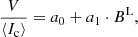
We inferred the longitudinal component BL of the magnetic field strength in the weak field limit by applying Eq. (1) to the Stokes profiles of the Si I 10 827 Å line synthesized using the 3D MHD snapshot model of Rempel (2014). The top panels of Fig. 7 show the scatter of the Stokes V signals plotted against the inferred longitudinal component for three cases of spatial smearing. As seen in the figure, in the quiet solar areas represented by this model the Stokes V signal of the Si I 10 827 Å line measured at the wavelengths of the intensity derivative peak can be approximated rather well by a linear function of the longitudinal component BL:
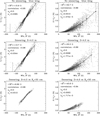 |
Fig. 7. Left: scatter plots of the Stokes V signal (small gray squares) in the blue wing of the Si I 10 827 Å line against the longitudinal component BL of the magnetic field for three cases of spatial resolution. Right: same, but for the linear polarization P and the transverse component BT of the magnetic field. The BL and BT values have been inferred from synthetic Stokes profiles of the Si I line using the weak field approximation (WFA). Top: original spatial resolution (no smearing effects). Middle: finite spatial resolution due to the diffraction limit of a 4 m telescope. Bottom: reduced resolution caused by the telescope and seeing (R0 = 50 cm) effects. The V and P signals were calculated at the wavelength where the modulus of the intensity derivative is maximum. Black circles and vertical lines indicate, respectively, averages and error bars over bins with 50 surface points. The thick solid curves represent the first-degree (left panels) and the second-degree (right panels) polynomial fits to these averages. The mean values of the transverse and the unsigned longitudinal components, the correlation coefficients and the coefficients of the polynomial fits are shown in the respective panels. The scatter plots were calculated using the 3D snapshot model of Rempel (2014) discussed in Sect. 2.1. |
where the coefficient a0 is equal to zero while the coefficient a1 depends on the spatial resolution, slightly changing from 0.0365 for unsmoothed Stokes profiles to 0.0312 for profiles affected by the telescope and seeing effects. The linear dependence of the Stokes V on the longitudinal component BL shown in Fig. 7 is confirmed by the high correlation coefficient between them that, depending on the degree of spatial smearing, ranges between 0.95 and 0.99. This linearity is indeed valid only in the limit of weak magnetic field. As follows from the top panels of Fig. 7, when the the longitudinal component BL increases, the scatter of the Stokes V signals becomes larger. This happens because with amplification of the magnetic field the Stokes V amplitude starts to depend not only on the BL value, but also on the angle θ between the magnetic field field vector and the line of sight (Landi Degl’Innocenti & Landolfi 2004). Another reason for such a scatter is connected with the fact that in the formation region of the Si I 10 827 Å line, as we have shown in Sect. 3, the condition of the field homogeneity required for the weak field approximation is not satisfied. Besides, the intensity derivative varies along the snapshot model surface.
The results shown in Fig. 7 confirm our conclusion of Sect. 4.1. It can be seen again that spatial smearing drastically reduces the Stokes V signal. The main consequence of this is the reduced strength of the inferred magnetic field. With deterioration in the spatial resolution of observations with a 4 m telescope the unsigned longitudinal component ⟨|BL|⟩ averaged over the surface of the model begins to decrease. For a spatial resolution of ∼0.54″ (R0 = 50 cm) it can be reduced by about a factor of two as compared with the case corresponding to the diffraction limit of this telescope (see top and bottom left panels of Fig. 7). We discuss this problem in detail in Sects. 4.4 and 4.5.
4.3. Stokes P versus the transverse component of the magnetic field
The right panels of Fig. 7 show the total linear polarization P of the Si I 10 827 Å line profile against the transverse component BT of the magnetic field strength for three cases of spatial resolution. We calculated the BT values in the weak field limit for all (x, y)-grid points of the 3D snapshot model using Eq. (2). The data shown in the right panels of Fig. 7 have been approximated by the second-degree polynomial:
where the coefficients b0, b1, b2 depend on the spatial resolution. We show them in the right panels of Fig. 7. We note that the correlation between BT and P, although smaller than in the case of the longitudinal component, still remains high varying from 0.88 to 0.94. As can be seen in this figure, when the transverse component BT increases, the scatter of the P signal calculated at the wavelength of the intensity derivative peaks is even larger than in the case of the longitudinal component. As in the case discussed in Sect. 4.2, this happens because with amplification of the magnetic field the P signal turns out to be a function of not only the transverse component, but also of the inclination angle θ (Landi Degl’Innocenti & Landolfi 2004). In addition, the surface variations of the intensity derivative and the changes of the field along the line-of-sight in the presence of velocity gradients affect the results obtained using the weak field approximation. This could be an another factor causing such a scatter.
The right panels of Fig. 7 demonstrate again that with a deterioration of spatial resolution, the mean transverse component ⟨BT⟩ decreases, similarly to the longitudinal component ⟨|BL|⟩ of the field, decreases. However, unlike the latter case, the effect on the transverse component is less pronounced.
4.4. Comparison of the magnetic field inferred using the weak field approximation with the magnetic field of the model
The weak field approximation does not allow to identify the photospheric layers where the Zeeman polarization produced by the magnetic field originates. In order to get an idea of this we assume that for a given wavelength Δλ within the Si I 10 827 Å line the information on the magnetic field comes from a single optical depth τΔλ = 1. In other words, we use the concept of “Eddington-Barbier height” (defined as the height where the optical depth is equal to one).
The top panels of Fig. 8 show the maps of the vertical (BZ) and horizontal (BXY) components of the magnetic field vector in the 3D model. These values were determined at the corrugated surface of constant optical depth τΔλ = 1, where Δλ is the wavelength location of the intensity derivative peaks in the blue wing of the Si I 10 827 Å line. We identify these maps with the magnetic field of the model.
 |
Fig. 8. Top, from left to right: variation of the vertical BZ and horizontal BXY components of the magnetic field strength in the 3D snapshot model throughout the corrugated surface where the line optical depth τΔλ = 1, Δλ being the wavelength location of the intensity derivative peaks. Second to fourth rows: maps of the longitudinal BL (left column) and transverse BT (right column) components of the magnetic fields obtained by applying the WFA to the synthetic Stokes profiles of the Si I 10 827 Å line, calculated for three cases of spatial resolution. The lower and upper limits of the inferred magnetic fields are indicated at the right side of the respective images. For more information see the caption of Fig. 6. |
We compare the above-mentioned maps with the corresponding maps of the longitudinal BL and transverse BT components of the field that were inferred from the synthesized Stokes profiles of the Si I 10 827 Å line using the weak field approximation. The second, third, and fourth rows of Fig. 8 show such maps for three cases of spatial resolution.
The results presented in the top and second-row panels clearly indicate that at full resolution the topology of the field on the corrugated surface where the optical depth τΔλ = 1 and that obtained with the weak field approximation are almost identical, except that the longitudinal and transverse components derived with the WFA are smaller in magnitude. The latter is easy to understand bearing in mind that the weak field approximation gives average information over a certain height range, thus leading to a decrease in the inferred magnetic field amplitude. Figure 8 shows that the agreement between the “real” and the inferred magnetic fields continues to be good when using spatially smeared Stokes profiles corresponding to the diffraction resolution of a 4 m telescope (see panels in the third row of Fig. 8). Even under poor seeing conditions (see the bottom panels), the structure of the “real” field is still traced.
In order to better quantify the extent to which the layer associated with the longitudinal and transverse components shown in Fig. 8 are close to the “Eddington-Barbier height” we compared the probability density functions (PDF) for the BL and BT components corresponding to the unsmeared case with the PDF of the “real” field of the 3D snapshot model. It is important to note that the observed Stokes profiles are degraded by photon noise, and this has an impact on the accuracy of the determination of the solar magnetic fields (e.g., Pietarila Graham et al. 2010; Danilovic et al. 2010; Stenflo 2010; Borrero & Kobel 2011, 2012, and more details therein).
To study how sensitive the PDFs for the BL and BT components are to such effects we added noise to the Stokes profiles as a normally distributed random variable with a standard deviation σ = 3 × 10⁻⁴. As noted in Sect. 4.1, this value represents a three-times-higher noise level than in the observations obtained by Martínez González et al. (2016). Figure 9 shows the PDFs for the BL and BT components of the magnetic field derived from the noise-free and the noisy Stokes profiles in the weak field limit. For comparison, we also present the BZ and BXY components taken from the 3D snapshot model of Rempel (2014).
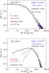 |
Fig. 9. Top: probability density functions (PDF) for the unsigned longitudinal BL (dashed and dot-dashed curves) and the unsigned vertical BZ (solid curve) components of the magnetic field vector in the 3D snapshot model of Rempel (2014). Bottom: same but for the transverse BT and the horizontal BXY components of the magnetic field. The BL and BT values have been inferred from the unsmeared Stokes signals at the blue wing of the Si I 10 827 Å line using the weak field approximation. Dashed and dot-dashed curves correspond to the noise-free and the noisy Stokes profiles, respectively. The BZ and BXY values are, respectively, the vertical and horizontal components of the magnetic field of the model taken at the corrugated surface of optical depth τΔλ = 1, where Δλ is the wavelength location of the intensity derivative peaks in the blue wing of the Si I 10 827 Å line. |
As seen in Fig. 9, the unsigned noise-free |BL| and |BZ| distributions follow each other closely, except mainly for the strongest signals; for such signals the mean unsigned longitudinal component turns out to be smaller than the mean unsigned vertical field while the correlation between these two components still remains high.
The top panel of Fig. 9 also shows that both the noise-free and noisy |BL| distributions for the case σ = 3 × 10⁻⁴ almost coincide. In addition to this, we found that the presence of the noise does not affect the “Eddington-Barbier height” where the Zeeman polarization originates. This gives us reason to conclude that the BL and BT inferred from the Si I 10827 Å line can be associated with the “Eddington-Barbier” layer. The mean height of this layer is ⟨H⟩=317 km.
In contrast, the discrepancies between PDFs for the transverse BT and the horizontal BXY components of the magnetic field are most pronounced for the weak linear polarization signals. The presence of noise in spectropolarimetric observations increases such discrepancies even more. Furthermore, the probability distribution function for the transverse component becomes more peaked. Moreover, the difference between the mean transverse and horizontal components increases and the correlation between them becomes worse.
4.5. Dependence of the retrieved magnetic field on the seeing conditions and telescope diameter
Until now we have discussed the advantages and disadvantages of the weak field approximation only for the case of a large-diameter telescope (D = 4 m) and only for one case of spatial resolution characterized by the Fried parameter R0 = 50 cm. This parameter corresponds to a spatial resolution ∼0.54″ and a rms continuum contrast δIrms close to ∼4.5% at the wavelength λ = 10827 Å (see Fig. 2). We now consider what happens if telescopes with different apertures are used under different seeing conditions.
Figure 10 helps to answer this question. Under poor seeing conditions corresponding to a spatial resolution of about 1″ or worse the choice of telescope on which the observations are obtained has little effect. For telescopes with diameters of 4 m, 1.5 m, and 0.7 m the mean retrieved longitudinal ⟨|BL|⟩ and transverse ⟨BT⟩ components of the field remain the same and significantly smaller than those obtained from the unsmeared Stokes profiles (we note that the mean ⟨|BL|⟩ and ⟨BT⟩ values for the unsmeared case are shown in the top and bottom panels of Fig. 10, respectively). The diameter of the telescope becomes important for spatial resolutions better than 0.5″, which corresponds to a Fried parameter R0 ≥ 50 cm and a rms continuum contrast δIrms ≥ 5% for D = 4 m. Figure 10 shows that for the best resolution (0.27″) that the GREGOR Infrared Spectrograph can achieve for NIR wavelengths close to the Si I line (see Joshi et al. 2016) the ⟨|BL|⟩ and ⟨BT⟩ values are 8.3 G and 43.3 G, respectively.
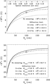 |
Fig. 10. Top: mean unsigned longitudinal component ⟨|BL|⟩ of the magnetic field in the weak field limit as a function of the Fried parameter R0 at the wavelength λ = 10 827 Å. Bottom: same but for the mean transverse component ⟨BT⟩ of the magnetic field. Solid, dashed, and dotted curves correspond to telescope diameters 4 m, 1.5 m, and 0.7 m, respectively. Open circles indicate the ⟨|BL|⟩ and ⟨BT⟩ values for the best resolution that the GREGOR Infrared Spectrograph can achieve at 10 832 Å (Joshi et al. 2016). The rms continuum contrast δIrms, as well as the ⟨|BL|⟩ and ⟨BT⟩ values for the spatial resolution of the 3D model (no smearing and no noise effects) and for reduced resolutions due to the telescope diffraction are shown in the panels. We note that the mean vertical ⟨|BZ|⟩ and transverse ⟨|BXY|⟩ components of the model are equal to 25.7 G and =49.5 G, respectively. The top horizontal axis gives the spatial resolution, corresponding to the Fried parameter R0 shown in the bottom horizontal axis. |
Under excellent seeing conditions the difference between the mean ⟨|BL|⟩ values obtained using telescopes with diameters of 1.5 m and 4 m are noticeably smaller in comparison with such difference when using telescopes with diameters of 0.7 m and 1.5 m, or of 0.7 m and 4 m. Similar differences are also found for the transverse ⟨BT⟩ field component. Finally, in the weak field limit the ⟨|BL|⟩ and ⟨BT⟩ values inferred from diffraction limited observations with a 4 m telescope turn out to be very close to their limiting values that can be retrieved from the unsmeared data. At the same time, the ⟨|BL|⟩ value remains noticeably smaller than the mean vertical component of the model: ⟨|BZ|⟩=25.7 G. Concerning the transverse component, the ⟨BT⟩ value for such observations is consistent with the mean horizontal component of the model: ⟨|BXY|⟩=49.5 G.
5. Conclusions
We investigated the validity of the weak field approximation for the Si I 10 827 Å line. To this end, we used a 3D snapshot model of the quiet solar atmosphere taken from a magneto-convection simulation with small-scale dynamo action (see Rempel 2014). We calculated the NLTE Stokes I, Q, U, and V profiles of this line at the solar disk center for every surface point of the 3D model. We retrieved the magnetic properties of the model applying the weak field approximation to the calculated Stokes profiles produced by the Zeeman effect and compared the inferred transverse and longitudinal components of the magnetic field with the original horizontal and vertical model values. Finally, we estimated the extent to which the diffraction limit of the telescope, the photon noise, and seeing affect the recovered magnetic field values. To this end, we calculated the mean transverse and the mean unsigned longitudinal values as a function of the Fried parameter R0 for the apertures of the VTT, GREGOR, and EST/DKIST telescopes. The results presented in this paper were obtained by analyzing the polarization in the blue wing of the Si I 10 827 Å line where significant V/Ic and P/Ic values are found. The results for the red wing are very similar.
We conclude that the weak field approximation can be applied for understanding the Zeeman polarization signals of the Si I 10 827 Å line observed in quiet regions of the solar atmosphere. We found that in these regions the Stokes V signals of the Si I 10 827 Å line can be described rather well by a linear dependence on the longitudinal component of the magnetic field strength and by a quadratic dependence for the total linear polarization P on the transverse component.
It is crucial to observe the polarization of the Si I 10 827 Å line under the best possible spatial resolution, clearly better than 0.5″. For worse resolutions, the Stokes V and P signals are significantly reduced. As a result, the mean values of the inferred transverse and unsigned longitudinal components are reduced in a similar way.
Under excellent seeing conditions the surface maps of the magnetic field inferred from the Si I line using the weak field approximation are close to the maps of the real field found at the corrugated surface where the optical depth τΔλ = 1. The correlation between them is relatively high, except that the longitudinal and transverse components of the magnetic field strength are systematically lower than vertical and horizontal components.
In summary, under high-spatial-resolution conditions, the weak field approximation applied to spectropolarimetric observations of the Si I 10 827 Å line using telescopes with apertures like those of GREGOR, EST, and DKIST provides reasonable information on the photospheric magnetic field strength, with the accuracy of the inferred values decreasing with the diameter of the telescope used.
Finally, it is interesting to note that the Zeeman polarization signal in the wings of the Si I 10 827 Å line is sensitive to the same solar photospheric layers as the scattering polarization in the Sr I 4 607 Å (see, e.g., Trujillo Bueno et al. 2004; Trujillo Bueno & Shchukina 2007; Shchukina & Trujillo Bueno 2011; del Pino Alemán et al. 2018). This opens up new opportunities for the study of the small-scale magnetic activity in the middle photosphere where these polarization signals are formed.
Acknowledgments
We are grateful to M. Rempel (HAO) for providing the 3D model atmosphere we have used in this investigation. N.S. is grateful to the Fundaci Jesús Serra Visiting Researchers Programme of the IAC for financing a three months working visit at the IAC. J.T.B. acknowledges the funding received from the European Research Council (ERC) under the European Union’s Horizon 2020 research and innovation programme (ERC Advanced Grant agreement No 742265).
References
- Balthasar, H., Gömöry, P., González Manrique, S. J., et al. 2018, ArXiv e-prints [arXiv:1804.01789] [Google Scholar]
- Bard, S., & Carlsson, M. 2008, ApJ, 682, 1376 [NASA ADS] [CrossRef] [Google Scholar]
- Borrero, J. M., & Kobel, P. 2011, A&A, 527, A29 [NASA ADS] [CrossRef] [EDP Sciences] [Google Scholar]
- Borrero, J. M., & Kobel, P. 2012, A&A, 547, A89 [NASA ADS] [CrossRef] [EDP Sciences] [Google Scholar]
- Borrero, J. M., Lites, B. W., Lagg, A., Rezaei, R., & Rempel, M. 2014, A&A, 572, A54 [NASA ADS] [CrossRef] [EDP Sciences] [Google Scholar]
- Collados, M., López, M., Páez, R., et al. 2012, Astron. Nachr., 333, 872 [NASA ADS] [CrossRef] [Google Scholar]
- Collados, M., Bettonvil, F., Cavaller, L., et al. 2013, in Highlights of Spanish Astrophysics VII, eds. J. C. Guirado, L. M. Lara, V. Quilis, & J. Gorgas, 808 [Google Scholar]
- Danilovic, S., Schüssler, M., & Solanki, S. K. 2010, A&A, 513, A1 [NASA ADS] [CrossRef] [EDP Sciences] [Google Scholar]
- del Pino Alemán, T., Štěpán, J., Trujillo, Bueno J., & Shchukina, N. 2018, ApJ, 863, 164 [NASA ADS] [CrossRef] [Google Scholar]
- del Toro, Iniesta J. C., & Ruiz Cobo, B. 2006, Sol. Phys., 13, 4 [Google Scholar]
- Denker, C., Lagg, A., Puschmann, K. G., et al. 2012, IAU Spec. Sess., 6 [Google Scholar]
- Felipe, T., Collados, M., Khomenko, E., et al. 2016, A&A, 596, A59 [NASA ADS] [CrossRef] [EDP Sciences] [Google Scholar]
- Fried, D. L. 1966, J. Opt. Soc. Am., 56, 1372 [NASA ADS] [CrossRef] [Google Scholar]
- Frutiger, C., Solanki, S. K., Fligge, M., et al. 2000, A&A, 358, 1109 [Google Scholar]
- Grevesse, N., & Sauval, A. J. 1998, in Solar Composition and its Evolution – from Core to Corona, eds. C. Frolich, M. Huber, S. K. Solanki, & R. von Steiger (Dordrecht: Kluwer), 161 [CrossRef] [Google Scholar]
- Illing, R. M. E., Landman, D. A., & Mickey, D. L. 1975, A&A, 41, 183 [NASA ADS] [Google Scholar]
- Joshi, J., Lagg, A., Solanki, S. K., et al. 2016, A&A, 596, A8 [NASA ADS] [CrossRef] [EDP Sciences] [Google Scholar]
- Keil, S. L., Rimmele, T. R., Wagner, J., Elmore, D., & ATST Team 2011, ASP Conf. Ser., 437, 319 [Google Scholar]
- Khomenko, E. 2006, ASP Conf. Ser., 354, 63 [Google Scholar]
- Khomenko, E. V., Collados, M., Solanki, S. K., Lagg, A., & Trujillo Bueno, J. 2003, A&A, 408, 1115 [NASA ADS] [CrossRef] [EDP Sciences] [Google Scholar]
- Khomenko, E. V., Shelyag, S., Solanki, S. K., & Vögler, A. 2005, A&A, 442, 1059 [NASA ADS] [CrossRef] [EDP Sciences] [Google Scholar]
- Korff, D. 1973, J. Opt. Soc. Am., 63, 971 [NASA ADS] [CrossRef] [Google Scholar]
- Kuckein, C., Martínez Pillet, V., & Centeno, R. 2012, A&A, 542, A112 [NASA ADS] [CrossRef] [EDP Sciences] [Google Scholar]
- Kuckein, C., Collados, M., & Manso Sainz, R. 2015, ApJ, 799, L25 [NASA ADS] [CrossRef] [Google Scholar]
- Lagg, A., Woch, J., Krupp, N., & Solanki, S. K. 2004, A&A, 414, 1109 [NASA ADS] [CrossRef] [EDP Sciences] [Google Scholar]
- Landi Degl’Innocenti, E., & Landolfi, M. 2004, Polarization in Spectral Lines (Kluwer Academic Publishers) [Google Scholar]
- Martínez González, M. J., Pastor Yabar, A., Lagg, A., et al. 2016, A&A, 596, A5 [NASA ADS] [CrossRef] [EDP Sciences] [Google Scholar]
- Matthews, S. A., Collados, M., Mathioudakis, M., & Erdelyi, R. 2016, SPIE Conf. Ser., 9908, 990809 [Google Scholar]
- Orozco Suárez, D., Quintero Noda, C., Ruiz Cobo, B., & Collados Vera, M. 2017, A&A, 607, A102 [NASA ADS] [CrossRef] [EDP Sciences] [Google Scholar]
- Penn, M. J. 2014, Sol. Phys., 11, 2 [Google Scholar]
- Pietarila Graham, J., Danilovic, S., & Schüssler, M. 2010, ApJ, 693, 1728 [Google Scholar]
- Rempel, M. 2014, ApJ, 789, 132 [NASA ADS] [CrossRef] [Google Scholar]
- Rüedi, I., Solanki, S. K., & Livingston, W. C. 1995, A&A, 293, 252 [NASA ADS] [Google Scholar]
- Ruiz Cobo, B., & del Toro Iniesta, J. C. 1992, ApJ, 398, 375 [NASA ADS] [CrossRef] [Google Scholar]
- Shchukina, N., & Trujillo Bueno, J. 2001, ApJ, 550, 970 [NASA ADS] [CrossRef] [Google Scholar]
- Shchukina, N., & Trujillo Bueno, J. 2011, ApJ, 731, L21 [NASA ADS] [CrossRef] [Google Scholar]
- Shchukina, N. G., & Trujillo Bueno, J. 2013, Proc. IAU Symp., 294, 107 [NASA ADS] [Google Scholar]
- Shchukina, N., & Trujillo Bueno, J. 2015, A&A, 579, A112 [NASA ADS] [CrossRef] [EDP Sciences] [Google Scholar]
- Shchukina, N. G., Olshevsky, V. L., & Khomenko, E. V. 2009, A&A, 506, 1393 [NASA ADS] [CrossRef] [EDP Sciences] [Google Scholar]
- Shchukina, N., Sukhorukov, A., & Trujillo Bueno, J. 2012, ApJ, 755, 176 [NASA ADS] [CrossRef] [Google Scholar]
- Shchukina, N., Sukhorukov, A., & Trujillo Bueno, J. 2017, A&A, 603, A98 [NASA ADS] [CrossRef] [EDP Sciences] [Google Scholar]
- Socas-Navarro, H., de la Cruz Rodríguez, J., Asensio Ramos, A., Trujillo Bueno, J., & Ruiz Cobo, B. 2015, A&A, 577, A7 [NASA ADS] [CrossRef] [EDP Sciences] [Google Scholar]
- Stenflo, J. O. 2010, A&A, 517, A37 [NASA ADS] [CrossRef] [EDP Sciences] [Google Scholar]
- Stenflo, J. O., Harvey, J. W., Brault, J. W., & Solanki, S. K. 1984, A&A, 131, 333 [NASA ADS] [Google Scholar]
- Solanki, S. K. 1993, Space Sci. Rev., 63, 1 [NASA ADS] [CrossRef] [Google Scholar]
- Solanki, S., Lagg, A., Woch, J., Krupp, N., & Collados, M. 2003, Nature, 425, 692 [NASA ADS] [CrossRef] [PubMed] [Google Scholar]
- Soltau, D., Volkmer, R., von der Lühe, O., & Berkefeld, T. 2012, Astron. Nachr., 333, 847 [NASA ADS] [CrossRef] [Google Scholar]
- Sukhorukov, A. V. 2012, J. Phys. Stud., 16, 1903 [Google Scholar]
- Sukhorukov, A. V., & Shchukina, N. G. 2012, Kinemat. Phys. Celest. Bodies, 28, 169 [NASA ADS] [CrossRef] [Google Scholar]
- Trujillo Bueno, J. 2003, ASP Conf. Ser., 288, 551 [NASA ADS] [Google Scholar]
- Trujillo Bueno, J., & Landi Degl’Innocenti, E. 1996, Sol. Phys., 164, 135 [NASA ADS] [CrossRef] [Google Scholar]
- Trujillo Bueno, J., & Shchukina, N. 2007, ApJ, 664, L135 [NASA ADS] [CrossRef] [Google Scholar]
- Trujillo Bueno, J., Shchukina, N., & Asensio Ramos, A. 2004, Nature, 430, 326 [Google Scholar]
- Wiegelmann, T., Lagg, A., Solanki, S. K., Inhester, B., & Woch, J. 2005, A&A, 433, 701 [NASA ADS] [CrossRef] [EDP Sciences] [Google Scholar]
- Xu, Z., Lagg, A., Solanki, S., & Liu, Y. 2012, ApJ, 749, 138 [NASA ADS] [CrossRef] [Google Scholar]
- Yelles Chaouche, L., Kuckein, C., Martínez Pillet, V., & Moreno-Insertis, F. 2012, ApJ, 748, 23 [NASA ADS] [CrossRef] [Google Scholar]
All Figures
|
Fig. 1. Histograms of the NLTE heights of formation calculated at four wavelengths within the Si I 10 827 Å line intensity profile. The top horizontal axis gives the mean optical depths ⟨τ5⟩ corresponding to the heights shown in the bottom horizontal axis. The mean heights of formation and wavelengths are shown close to each of the histograms. The histograms were calculated using the 3D snapshot model with ⟨|BZ|⟩ = 80 G (Rempel 2014) and the Si I model with six bound-bound transitions described by Shchukina et al. (2017). |
| In the text | |
|
Fig. 2. Root-mean-square continuum contrast δIrms as a function of the Fried parameter R0 at wavelength λ = 10827 Å. Dotted, dashed, and solid curves correspond to the telescope diameters 0.7, 1.5, and 4 m, respectively. The δIrms contrast for observations affected only by the diffraction limit of the VTT(D = 0.7 m), GREGOR (D = 1.5 m) and EST/DKIST (D = 4.0 m) telescopes (no seeing effects) are indicated in the upper part of this figure. The vertical arrow in the lower right corner marks the δIrms value for the “perfect” observations corresponding to the case of the original spatial resolution (no smearing caused by the telescope and seeing effects). The calibration curves for the determination of the Fried parameter R0 were calculated using the radiative transfer formal solution for the continuum intensity in the chosen 3D snapshot model of Rempel (2014). |
| In the text | |
|
Fig. 3. Left, from top to bottom: disk-center profiles of the intensity I, intensity derivative |
| In the text | |
|
Fig. 4. Top: histogram of wavelength positions of the unsigned Stokes |V| peaks of the Si I 10 827 Å line formed in the 3D snapshot model of Rempel (2014). Bottom: same but the for the unsigned intensity derivative |
| In the text | |
|
Fig. 5. Top: histogram of the zero-crossing wavelength positions of the Stokes V profiles of the Si I 10 827 Å line formed in the 3D snapshot model. Bottom: same but for the intensity derivative. Arrows and numbers indicate the mean values of such zero-crossing positions. |
| In the text | |
|
Fig. 6. From left to right: maps of the intensity derivative |
| In the text | |
|
Fig. 7. Left: scatter plots of the Stokes V signal (small gray squares) in the blue wing of the Si I 10 827 Å line against the longitudinal component BL of the magnetic field for three cases of spatial resolution. Right: same, but for the linear polarization P and the transverse component BT of the magnetic field. The BL and BT values have been inferred from synthetic Stokes profiles of the Si I line using the weak field approximation (WFA). Top: original spatial resolution (no smearing effects). Middle: finite spatial resolution due to the diffraction limit of a 4 m telescope. Bottom: reduced resolution caused by the telescope and seeing (R0 = 50 cm) effects. The V and P signals were calculated at the wavelength where the modulus of the intensity derivative is maximum. Black circles and vertical lines indicate, respectively, averages and error bars over bins with 50 surface points. The thick solid curves represent the first-degree (left panels) and the second-degree (right panels) polynomial fits to these averages. The mean values of the transverse and the unsigned longitudinal components, the correlation coefficients and the coefficients of the polynomial fits are shown in the respective panels. The scatter plots were calculated using the 3D snapshot model of Rempel (2014) discussed in Sect. 2.1. |
| In the text | |
|
Fig. 8. Top, from left to right: variation of the vertical BZ and horizontal BXY components of the magnetic field strength in the 3D snapshot model throughout the corrugated surface where the line optical depth τΔλ = 1, Δλ being the wavelength location of the intensity derivative peaks. Second to fourth rows: maps of the longitudinal BL (left column) and transverse BT (right column) components of the magnetic fields obtained by applying the WFA to the synthetic Stokes profiles of the Si I 10 827 Å line, calculated for three cases of spatial resolution. The lower and upper limits of the inferred magnetic fields are indicated at the right side of the respective images. For more information see the caption of Fig. 6. |
| In the text | |
|
Fig. 9. Top: probability density functions (PDF) for the unsigned longitudinal BL (dashed and dot-dashed curves) and the unsigned vertical BZ (solid curve) components of the magnetic field vector in the 3D snapshot model of Rempel (2014). Bottom: same but for the transverse BT and the horizontal BXY components of the magnetic field. The BL and BT values have been inferred from the unsmeared Stokes signals at the blue wing of the Si I 10 827 Å line using the weak field approximation. Dashed and dot-dashed curves correspond to the noise-free and the noisy Stokes profiles, respectively. The BZ and BXY values are, respectively, the vertical and horizontal components of the magnetic field of the model taken at the corrugated surface of optical depth τΔλ = 1, where Δλ is the wavelength location of the intensity derivative peaks in the blue wing of the Si I 10 827 Å line. |
| In the text | |
|
Fig. 10. Top: mean unsigned longitudinal component ⟨|BL|⟩ of the magnetic field in the weak field limit as a function of the Fried parameter R0 at the wavelength λ = 10 827 Å. Bottom: same but for the mean transverse component ⟨BT⟩ of the magnetic field. Solid, dashed, and dotted curves correspond to telescope diameters 4 m, 1.5 m, and 0.7 m, respectively. Open circles indicate the ⟨|BL|⟩ and ⟨BT⟩ values for the best resolution that the GREGOR Infrared Spectrograph can achieve at 10 832 Å (Joshi et al. 2016). The rms continuum contrast δIrms, as well as the ⟨|BL|⟩ and ⟨BT⟩ values for the spatial resolution of the 3D model (no smearing and no noise effects) and for reduced resolutions due to the telescope diffraction are shown in the panels. We note that the mean vertical ⟨|BZ|⟩ and transverse ⟨|BXY|⟩ components of the model are equal to 25.7 G and =49.5 G, respectively. The top horizontal axis gives the spatial resolution, corresponding to the Fried parameter R0 shown in the bottom horizontal axis. |
| In the text | |
Current usage metrics show cumulative count of Article Views (full-text article views including HTML views, PDF and ePub downloads, according to the available data) and Abstracts Views on Vision4Press platform.
Data correspond to usage on the plateform after 2015. The current usage metrics is available 48-96 hours after online publication and is updated daily on week days.
Initial download of the metrics may take a while.