| Issue |
A&A
Volume 628, August 2019
|
|
|---|---|---|
| Article Number | A82 | |
| Number of page(s) | 21 | |
| Section | Numerical methods and codes | |
| DOI | https://doi.org/10.1051/0004-6361/201833143 | |
| Published online | 09 August 2019 | |
Self-gravitating disks in binary systems: an SPH approach
I. Implementation of the code and reliability tests
1
Dipartimento di Fisica, Sapienza, Università di Roma, P.le Aldo Moro, 5, 00185 Rome, Italy
e-mail: This email address is being protected from spambots. You need JavaScript enabled to view it.
2
INAF-IAPS, Istituto di Astrofisica e Planetologia Spaziali, Area di Ricerca di Tor Vergata, Via del Fosso del Cavaliere, 100, 00133 Rome, Italy
Received:
2
April
2018
Accepted:
19
June
2019
Abstract
The study of the stability of massive gaseous disks around a star in a nonisolated context is a difficult task and becomes even more complicated for disks that are hosted by binary systems. The role of self-gravity is thought to be significant when the ratio of the disk-to-star mass is non-negligible. To solve these problems, we implemented, tested, and applied our own smoothed particle hydrodynamics (SPH) algorithm. The code (named GaSPH) passed various quality tests and shows good performances, and it can therefore be reliably applied to the study of disks around stars when self-gravity needs to be accounted for. We here introduce and describe the algorithm, including some performance and stability tests. This paper is the first part of a series of studies in which self-gravitating disks in binary systems are let evolve in larger environments such as open clusters.
Key words: protoplanetary disks / hydrodynamics / binaries: general
© ESO 2019
1. Introduction
The study of protoplanetary disks in nonisolated system has become a relevant topic in numerical astrophysics because several planetary systems and disks around stars inside open clusters have recently been observed. The recent discovery of a Neptune-sized planet that is hosted by a binary star in the nearby Hyades cluster (Ciardi et al. 2018) has opened new perspectives for the study of the evolution of primordial disks that interact with binary stars in a nonisolated environment. In the context of the study of isolated binary systems, we note that most of the classical models have studied low-mass disks, with the result that even considering their self-gravity, no appreciable change is observed in the time evolution of the stellar orbital parameters. Additionally, low-mass disks give a poor feedback on the hosting stars, which means that the timescale for the variation in their orbital parameters is larger than the other dynamical timescales that are involved.
To investigate such systems, we built our own smoothed particle hydrodynamics (SPH) code to integrate the evolution of the composite star+gas system. Following the scheme described in Capuzzo-Dolcetta & Miocchi (1998), our code treats gravity by means of a classical tree-based scheme (see also Barnes 1986; Barnes & Hut 1986; Miocchi & Capuzzo-Dolcetta 2002) and adds a proper treatment of the close gravitational interactions of the gas particles. The evolution of a limited number of point-mass objects (which may represent either stars or planets) is treated with a high-order explicit method.
This preliminary work provides an instrument that is not only suited to modeling heavy protoplanetary disks that interact with single and binary stars. It can also be used to study these systems not in isolation, but in stellar systems such as open star clusters.
In the next section we describe our code after preliminarily introducing the numerical framework, and in Sect. 3 we present and discuss some physical and performance tests. In Sect. 4 we describe the disk model we adopted and the application of our code to the study of heavy Keplerian disks. Section 5 is dedicated to the conclusions.
2. Numerical algorithm
In order to study a selg-gravitating gas, we developed an SPH code, coupled with a tree-based scheme for the Newtonian force integration. In this section, after a breaf recall of some basic theory of gravitational tree codes and of the SPH formalism (Sect. 2.1), we describe the main features of our numerical algorithm (Sect. 2.2). For further technical details, we refer to Appendices A.1 and A.2.
2.1. Basic theory
Introduced for the first time by Lucy (1977) and Gingold & Monaghan (1977), the SPH scheme has been widely adopted to investigate a huge set of astronomical problems that involve fluid systems. An SPH scheme allows integrating the fluid dynamical equations in a Lagrangian approach by representing the system through a set of points, or so-called pseudo-particles. For each particle, a set of fundamental quantities (such as density ρ, pressure P, internal energy u, and velocity v) are calculated by means of an interpolation with a proper kernel function over a suitable neighbor. For an exhaustive explanation of the method, we refer to various papers in the literature, such as those by Monaghan & Lattanzio (1985), Monaghan (1988, 2005). Here we recall some basic aspects.
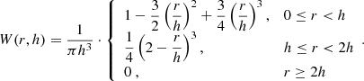
Interpolations are performed with a continuous kernel function W(r, h), whose spread scale is determined by a characteristic length h, called the smoothing length. It can easily be shown (see, e.g., Hernquist & Katz 1989) that under some additional constraints, interpolation errors are limited to the order O(h2). We used as kernel function the cubic spline that was for the first time adopted by Monaghan & Lattanzio (1985), who developed a formalism that had been introduced by Hockney & Eastwood (1981). This kernel function has the following form:
 (1)
(1)
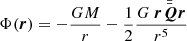
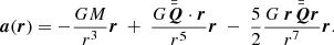
The SPH interpolation involves only a limited set of N′ neighboring particles that are enclosed within the range 2h, therefore the computational effort is expected to scale linearly with the total particle number N. On the other hand, when long-range interactions such as gravity are considered, the computational effort increases because each particle interacts with the whole system. A classical direct N-body code would therefore require a computational weight scaling as N2. However, a suitable gravitational tree-based scheme allows us to efficiently evaluate the Newtonian force by approximating the potential with a harmonic expansion (see Barnes & Hut 1986; Barnes 1986, for a full explanation). For each particle, only the contribution from a local neighborhood is calculated through a direct particle–particle coupling, while the contribution from farther particles is suitably approximated. The following expressions (Eqs. (2) and (3)) represent the approximated potential Φ(r) and the force (per unit mass) a(r)= − ∇Φ(r) given by a far cluster of particles,
 (2)
(2)
 (3)
(3)
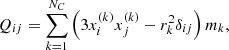
M is the total mass of this ensemble, r = |r| is the distance of the particle under study to the center of mass of the cluster. The symbol  represents the so-called quadrupole tensor, which is associated with the specific cluster. In indexed form, it is given by
 (4)
(4)
where  and
and  (i, j = 1, 2, 3) refer to the Cartesian coordinates of the kth particle of mass mk. The summation is performed over all the NC particles that are included in the cluster.
In the following section we describe the main structure and formalism used by GaSPH. Further computational details related to the implementation of the algorithm can be found in Appendices A and B.
2.2. Main structure of the algorithm
A single step to compute the acceleration contains two preliminary phases. One cycle is dedicated to map the particles into an octal grid domain. A further cycle, linear in N, is needed to evaluate some key parameters such as the density, ρ, the smoothing length, h, and the pressure, P. Then a third set of operations, the most complicated operation, is that of evaluating the gravitational and hydrodynamical forces in addition to the internal energy rate  of the gas.
GaSPH can also easily treat a system that consists of a set of point masses. To do this, the part of the SPH computations is turned off and the tree scheme alone is used for gravity interactions. On the other hand, a gas can be treated with pure hydrodynamics by turning off the gravitational field and using the SPH formalism alone.
After the main computations of the acceleration a and the energy rate  , the algorithm updates in time the velocity, position, and internal energy of the gas with a second-order Verlet method. Because of the structure of the second-order technique, the three main computational cycles should be performed twice into a single time iteration to obtain two estimates of a and
  .
.
In addition, the smooth particles may interact with a small number Nob of additional objects, an ensemble of point masses that mimic stars and/or planets. Differently from the other particles, the motion of these few objects is integrated with a 14th-order Runge–Kutta method by direct particle-to-particle N-body interactions without any approximation for the gravitational field. When Nob is sufficiently small, these operations request a little additional computational effort that scales roughly linearly with respect to the total number of points (including both the SPH particles number N and the objects number Nob). For the specific purpose of our investigation, where we have Nob ≤ 2, the general efficiency of the code is not affected.
2.2.1. Particle mapping and density computation
For a set of N equal-mass points, we preliminarily need to subdivide the system into a hierarchical series of subgroups of points in order to apply the multipole approximation for the Newtonian field contribution given by a “cluster”. To do this, we use a classical Barnes-Hut tree-code to map the particles into an octal grid space, according to their positions. We follow in particular the technique adopted by Miocchi & Capuzzo-Dolcetta (2002) by mapping the points through a 3-bit-based codification (see Sect. 2.2.6 for further details).
Before the accelerations are computed, SPH particles need a preliminary stage in which densities and smoothing lengths are computed. To perform a good interpolation, we need to keep a fixed number of neighbors for each point. For inhomogeneous fluids, we must therefore use a smoothing length h ≡ h(r, t) that varies in space and in time.
Individual smoothing lengths should be chosen in such a way that the higher the local number density n = ρ/m, the smaller the interpolation kernel radius: h ∝ n−1/3, in order to have a roughly constant number of neighbors of the given particle. For this purpose, we adopt a commonly used prescription (Hernquist & Katz 1989; Monaghan 2005). For each particle, we start from an initial guess for h, then we vary it until the number of particles that lie within the kernel dominion reaches a fixed value N0. We iterate a process in which each time the number of neighbor points, N′, is counted using a certain smoothing length hprev, then we update this length to a new value hnew according to the following formula:
![Mathematical equation: $$ \begin{aligned} h_{\mathrm{new}} = h_{\mathrm{prev}} \dfrac{1}{2} \left[ 1+\left( \dfrac{N_0}{N\prime }\right)^{1/3} \right] . \end{aligned} $$](/articles/aa/full_html/2019/08/aa33143-18/aa33143-18-eq11.gif) (5)
(5)
If the fluid were homogeneous, hprev(N0/N′)1/3 would immediately provide the correct value of the smoothing length, without any further iteration. The addend 1 lets the program perform an average of the old smoothing length, for which any excessive oscillation error due to non-homogeneities in the spatial distribution of particles is damped. The iteration is stopped when convergence is reached according to the criterion |N′−N0|≤ΔN, where ΔN is a tolerance number. In this regard, Attwood et al. (2007) investigated the acoustic oscillations of some models of polytrope around the equilibrium by imposing a constant neighbor number N′ and letting ΔN vary. They found that the fluctuation of N′±ΔN introduced an additional numerical noise that was able to break the stability of this system, giving rise to errors. To prevent errors, the authors found that ΔN should be set to zero, which is the choice we adopt in this paper. Moreover, they showed that the calculation of h according to the iterative process illustrated above and with ΔN = 0 is equivalent to solving for all the particles the 2N-equations system described by the following two equations:
 (6)
(6)
and to finding the exact solutions of density and smoothing length {ρi, hi | i ∈ [1, N]}, with  a suitable constant, and rij the mutual distance between the ith and the jth particles. We typically use a number of neighbors N′=60, such as δ ≈ 1.2.
When the density ρi is evaluated, the corresponding pressure Pi can be computed by means of a suitable equation of state. Appendix B.1 illustrates further technical details about the neighbor-search procedure.
2.2.2. Force calculation and softened interactions
For a generic ith particle, the acceleration ai is computed by adding both the SPH terms and the Newtonian terms in the same iteration. Together with the acceleration, the internal energy rate of the particle is also computed.
To treat a self-gravitating gas with an SPH scheme, a proper treatment of the gravitational potential is necessary to avoid overestimating the gravity field. Particles can be considered as point sources of the Newtonian field when their mutual distance is larger than 2h. Otherwise, their Newtonian interaction is, in consistency with the assumed kernel function (Gingold & Monaghan 1977), such that it vanishes at an interparticle distance approaching zero.
With the cubic spline kernel, we can obtain a different form of the Newtonian interaction between two particles, such that the classical term is softened if the particles approach within a distance of the order of a softening length ϵ = 2h. See the appendix in Hernquist & Katz (1989) for more details, and the appendix in Price & Monaghan (2007) for an explicit expression of the force and the potential. When SPH interaction is turned off, a constant value ϵ is generally used in place of 2h for the softening length. In this case, the total energy is conserved within the numerical error. On the other hand, the Hamiltonian becomes time dependent with SPH systems because the softening length varies in time, and so the energy is no longer conserved. To solve this problem, the equations of motion must be rewritten in a conservative form that takes the variation in h into account. We followed the Hamiltonian formalism as adopted for the first time by Springel & Hernquist (2002) for the hydrodynamical interactions, which was further developed by Price & Monaghan (2007) for the gravitational field. The SPH equation assume the form
![Mathematical equation: $$ \begin{aligned} \dfrac{\mathrm{d} \boldsymbol{v}_i}{\mathrm{d}t}&=- \sum \limits _{j} \frac{1}{2} \left( { g}_{\mathrm{soft}} (r_{ij},h_i) + { g}_{\mathrm{soft}} (r_{ij},h_j) \right) \frac{\boldsymbol{r}_{ij}}{r_{ij}}\nonumber \\&\quad - \sum \limits _{j} m_j \frac{G}{2} \left( \frac{\zeta _i}{\Omega _i} \boldsymbol{\nabla }_i W(r_{ij},h_i) + \frac{\zeta _j}{\Omega _j} \boldsymbol{\nabla }_i W(r_{ij},h_j) \right)\nonumber \\&\quad -\sum \limits _{j} m_j\left( \dfrac{P_i}{ \rho _i^2 \Omega _i} \boldsymbol{\nabla }_i W(r_{ij},h_i) + \dfrac{P_j}{ \rho _j^2 \Omega _j} \boldsymbol{\nabla }_i W(r_{ij},h_j) \right) \nonumber \\&\quad -\sum \limits _{j} m_j \Pi _{ij} \left[\frac{ \boldsymbol{\nabla _i} W(r_{ij},h_i) + \boldsymbol{\nabla }_i W(r_{ij},h_j) }{2}\right] +\dfrac{\mathrm{d} \boldsymbol{v}_{i}^{[\mathrm{stars}]}}{\mathrm{d}t} \end{aligned} $$](/articles/aa/full_html/2019/08/aa33143-18/aa33143-18-eq14.gif) (7)
(7)
 (8)
(8)
where the index i refers to a generic ith particle and the index j in the sums refers to the jth particle that is enclosed within the range 2hM = 2 ⋅ max(hi, hj). The term gsoft represents the softened gravitational force per unit mass mentioned above: it is a function only of the mutual particle distance rij and of the smoothing length h. It tends to zero as rij → 0 and assumes the classical Newtonian form  for rij ≥ 2h. The operator ∇i represents the gradient with respect to the coordinates of the ith particle. The gradient is performed over two different expressions of the kernel W, with two different lengths hi and hj. The terms ζi and Ωi are suitable functions that account for the variation in the smoothed Newtonian potential with respect to the softening length and for the non-uniformity of the softening length itself, respectively. They assume this form for a generic particle of index i:
 (9)
(9)
 (10)
(10)
where in the same way for the system in Eq. (6), the sum extends over the particles that are enclosed within the range 2hi. In Eq. (10), the function ϕsoft represents the softenend gravitational potential, such that ∇ϕsoft = −gsoftrij/rij. The potential reaches a constant value as rij → 0 and becomes equal to the Newtonian potential for rij ≥ 2h (for an explicit expression, see, e.g., Price & Monaghan 2007). Terms Ω and ζ are computed in the same neighbor-search iterative loop where ρ and h are worked out.
Only if the gas interacts with stars does the last term in Eq. (7), ![Mathematical equation: $ \mathrm{d} \boldsymbol{v}_{i}^{[\mathrm{stars}]}/\mathrm{d}t $](/articles/aa/full_html/2019/08/aa33143-18/aa33143-18-eq19.gif) (discussed in Sect. 2.2.4), represent a non-null acceleration that accounts for the Newtonian interaction between ith particle and the point masses. The function Πij, which we discuss in the following section, characterizes the well-known artificial viscosity. The expression of the equation of motion, Eq. (7), guarantees a symmetric exchange of linear momentum between the particles.
(discussed in Sect. 2.2.4), represent a non-null acceleration that accounts for the Newtonian interaction between ith particle and the point masses. The function Πij, which we discuss in the following section, characterizes the well-known artificial viscosity. The expression of the equation of motion, Eq. (7), guarantees a symmetric exchange of linear momentum between the particles.
2.2.3. Artificial viscosity
In high-compression regions such as shock wavefronts, the velocity gradient may be so strong that two layers interpenetrate and the hydrodynamical equations may not be integrated correctly and generate unphysical effects. Additional artificial pressure terms are a possible solution for this problem. In our code, we added an artificial term by adopting the same classical schematization as Monaghan (1989), which corresponds to introducing a suitable artificial viscosity that dampens the velocity gradient when two particles approach. Practically, a viscous-pressure term Πij is included in Eqs. (7) and (8). It assumes the expression
 (11)
(11)
where  . The dot product vij ⋅ rij involves the relative velocity and the distance of a pair of particles i − j. Only the particles that move in, for which vij ⋅ rij < 0, contribute to the artificial viscosity. The parameter η is a suitable term to prevent singularities when two particles approach very closely (we use the typical value of η = 0.1). The terms
  and
and  represent the average values of the smoothing length
  , the density
  and the speed of sound
  , respectively. We set β = 2α. In this simple formulation, the artificial viscosity is activated throughout the fluid; but in two circumstances it should be damped to prevent unphysical effects. Artificial viscosity must be damped in regions where shear dominates, and where the velocity gradient is low.
For two shearing layers of fluid, the relative velocity between the particles leads to an approach that is interpreted by the artificial viscosity (11) as a compression. This incorrect interpretation causes the code to overestimate the strength of the viscous interaction. To prevent false compressions, Balsara (1995) multiplied the term μij by a proper switching coefficient:
 (12)
(12)
in which the divergence of velocity and the velocity curl are evaluated for a particle of index i as
 (13)
(13)
We implemented the term f by multiplying μij for an average value 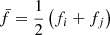 . Further problems may arise far away from high-compression regions. In the classical formulation of Πij, α = 1 = cost. (e.g., in Monaghan 1992). In this scheme, the viscosity acts with the same effectiveness in every region, while we would expect the artificial term to be efficient only where it is needed, that is, close to the shock fronts. To solve this problem, we used the same formalism as was introduced by Morris & Monaghan (1997) and further developed by Rosswog et al. (2000) by considering an individual αi for each particle that follows the time-variation equation,
 (14)
(14)
where Si = max(−(∇ ⋅ v)i, 0) (αmax − αmin) represents a “source” term that increases in the proximity of the shock front; αmin represents a minimum threshold value for α, and αmax represents its maximum. The (increasing) rate of the viscosity coefficient is driven by a characteristic timescale τα = hi/bcs that depends on how the fluid allows the perturbations to propagate through the resolution length. The individual viscosity coefficients αi and αj, when referred to a generic i − j particle pairing, are averaged in the same way as was done with the other quantities.
For a gas with γ = 5/3, a good value for the b coefficient can be set such that 5 ≤ b−1 ≤ 10 (Morris & Monaghan 1997). For our tests, we set αmax = 2, αmin = 0.1 and b−1 = 5. These are the most commonly adopted values in literature for a wide class of problems involving collapse, merging stars or protoplanetary disks (see, e.g., Rosswog & Price 2007; Stamatellos et al. 2011; Hosono et al. 2016). The implementation of the artificial viscosity term (Eqs. (12)–(14)), together with its form implemented in Eqs. (7) and (8), may affect the accuracy of the code in preserving the total angular momentum. In Sect. 3.1.5 we discuss how this form of viscosity, with different choices of the coefficients αmin and b, guarantees the conservation of the angular momentum.
2.2.4. Additional stellar objects
We calculated a direct point-to-point interaction for the mutual interaction between stars and to couple stars with SPH particles. The equation of motion of a generic p-th star takes the following form:
 (15)
(15)
where gsoft(r, ϵ) represents the Newtonian acceleration, which takes the form discussed above in Sect. 2.2.2. The force softening is accounted for the stars as well according to a constant softening length ϵs = cost. The gravity is thus softened when the mutual distance approaches ϵs. The first summation is extended over all SPH particles, while the index s in the second sum refers to the generic stars.
Similarly, the equation of motion, Eq. (7), when referred to a gas ith particle contains the following sum:
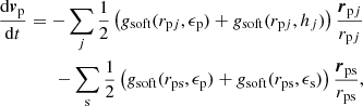
![Mathematical equation: $$ \begin{aligned} \dfrac{\mathrm{d} \boldsymbol{v}_i^{[\mathrm{stars}]}}{\mathrm{d}t} = - \sum \limits _{s} \frac{1}{2} \left( { g}_{\mathrm{soft}} ( r_{i\mathrm{s}} ,\epsilon _{\rm s}) + { g}_{\mathrm{soft}} (r_{i\mathrm{s}} ,h_i) \right) \frac{ \boldsymbol{r}_{i\mathrm{s}}}{r_{i\mathrm{s}} }, \end{aligned} $$](/articles/aa/full_html/2019/08/aa33143-18/aa33143-18-eq32.gif) (16)
(16)
where the index s again refers to the stars, and ris is the distance vector between a gas particle and a star.
2.2.5. Time integration and time-stepping
To evolve the gas system in time, we adopted a second-order integration method that is similar to a classical second-order Runge–Kutta scheme but is at the same time very similar to a leap-frog integrator: the well-known velocity-Verlet method (see Andersen 1983; Allen & Tildesley 1989, for detailed references). The Verlet method is based on a trapezoidal scheme coupled with a predictor-corrector technique for the estimation of v and u. The structure of this scheme is very similar to that of classical symplectic leap-frog algorithms, although it requires two computations of the force at every time iteration (see Appendix A.1). Nevertheless, the general velocity-Verlet method applied to gas evolution shows some advantages compared to the symplectic algorithm of the same order. Like a standard Runge–Kutta method, velocity and positions are updated in synchronized steps, without the Δt/2 shift. This feature provides a good flexibility in problems that are approached with nonuniform time-steps that involve the interaction of the gas component with other components that are integrated with different methods, as in our case. Various applications of velocity-Verlet methods in SPH schemes are found in the literature, for example, in Hubber et al. (2013) or in Hosono et al. (2016).
The additional point masses are ballistic elements, whose equation of motion needs to be integrated with very high precision to avoid secular trends that are typical of few-body gravitational problems. Although the SPH precision is at only second order, we decided to integrate the Newtonian motion of the (few) stars and planets in the system with a 14th-order Runge–Kutta method that was recently developed by Feagin (2012) through the so-called m-symmetry formalism. The method consists of 35 force computations per time-step, and in analogy with the well-known second- and fourth-order RK methods, it updates the velocities and the positions by suitable linear combinations of 35 different Kr and Kv coefficients (see Appendix A.2 for further details).
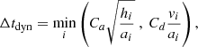
For the gas, we chose the time-step Δt following a criterion similar to the standard Courant–Friedrichs–Lewy (CFL) criterion that is commonly adopted for SPH systems (see, e.g., Monaghan 1992), together with some additional criteria. A global time-step Δtmin can be determined by taking the minimum between the following two quantities:
![Mathematical equation: $$ \begin{aligned} \Delta t_{\mathrm{term}} = \min \limits _i \left( \dfrac{C ~h }{c_{\mathrm{s} i} + h_i |\boldsymbol{\nabla }\cdot \boldsymbol{v}|_i + \varphi \alpha _i \left[ c_{\mathrm{s} i} + 2 \max \limits _{j}(\mu _{ij}) \right] } ~,~ C_{{u}} \dfrac{u_i }{\dot{u}_i } \right) \end{aligned} $$](/articles/aa/full_html/2019/08/aa33143-18/aa33143-18-eq33.gif) (17)
(17)
 (18)
(18)
where cs is the sound speed, C is a coefficient whose typical value lies between 0.1 and 0.4; we usually choose 0.15. Moreover, Cu, Ca, and Cd are coefficients to be set < 1. We chose Cu = 0.04, Ca = 0.15, and Cd = 0.02. Finally, the coefficient φ typically ranges from 0.6 to 1.2 (we adopt φ = 1.2 throughout). Similarly to the control of the variation in kinetic energy, we control the time variation of the thermal energy  in a single time-step by limiting it to a certain fraction Cu = 0.04. The index i refers to an individual time-step Δti that is related to a specific particle.
For the point-particle phase in the system (i.e., stars or planets), we chose a characteristic time-step, Δt, that is defined as
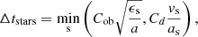 (19)
(19)
where we use Cob = 0.15. The various quantities with the index s of course characterize a specific star particle.
For a homogeneous medium, the integration can be performed with a global time-step, that is, the lowest value of gas and stars. Generally, the particles have different resolutions hi and different accelerations, which leads to a wide class of typical evolution timescales. For some particles, the integration might therefore be made with different Δti, which avoids the explicit force calculation at every time iteration and saves some computing time. We adopted a technique that was implemented in several N-body algorithms, such as the classical TREESPH (Hernquist & Katz 1989) or in the multi-GPU-parallelized N-body code HiGPUs (Capuzzo-Dolcetta et al. 2013). We assigned to each point a time-step as a negative two-power fraction of a reference time  (it can be a fixed quantity, or it may change periodically during the simulation). The particle motion is updated periodically according to their Δti in such a way that after an integration time Δtmax, all of them are synchronized (further details are explained in Appendix A.1). Particle mapping and sorting are performed every time for every particle as well, independently of their individual time-step. Thus, the configuration of the tree grid, together with total mass and quadrupole momentum of the boxes, are computed every single step Δtmin. Similarly, at each minimum time-step iteration, the gravitational interactions between gas and star are computed even during “inactive” stages of the gas. Thus, the acceleration of the inactive SPH particles is split into two terms: one is given by a fixed non-updated hydrodynamical and self-gravitaty term, and the other is given by a constantly updated gas-star gravitational force.
In our scheme, the stars and planets do not follow an individual time-step scheme, and their mutual interactions are computed for every single step Δtmin, even when Δtstars ≠ Δtmin. Furthermore, we force the particles that lie close to the stars within a tolerance distance to be integrated at every time iteration. Practically, we compute the distance for a generic ith particle from the stars, and we furthermore predict this distance at the following time iteration. When these values are lower than a tolerance of κϵob (with a constant κ ≥ 2), the particle time-step drops to Δtmin. For our practical purposes, we used a small number of objects (in the current investigation, Nob ≤ 2), thus, the 35-stage RK scheme requires a relatively short CPU-time (less than 2% of the total).
In gas problems that involve strong shocks, the use of individual time-steps may lead to strong errors. Even though CFL conditions are satisfied, the strong velocity gradients may determine a great discrepancy in time-steps between close particles. Consequently, close particles may evolve with very strongly different timescales. This may create too many asymmetries in the mutual hydrodynamical interactions, which causes unphysical discontinuities in velocity and pressure. Following the idea of Saitoh & Makino (2009), we limit for each pair of neighboring ith and jth particles the ratio of time-steps  . These investigators have shown that a good compromise is reached by the choice of A = 4, which gives good results without abruptly affecting the efficiency of the code.
2.2.6. Approximation of the gravitational field: opening criterion
The decomposition of the system into a series of clusters is performed by the tree algorithm through a recursive octal cube eight sub-boxes, each one subdivided into a further eight cubes of order L = 2, and so on. A tree structure is thus constituted, made of several nested boxes, each of which contains a group of particles. To calculate the acceleration of an ith particle, the algorithm walks along the tree, starting from the low-order cubes toward the highest order cubes (that contain just one particle), and evaluates the distance between the particle and the center of mass of the boxes. Each time a box is probed, the code decides to open it and probes its internal cubes only if the well-known opening criterion is satisfied,
 (20)
(20)
where θ is the so-called opening angle parameter for which reasonable values range among 0.3 and 1 (see Sect. 3.2, dedicated to performance tests), and DL = D0 × 2−L is the side length of the box. In the opposite case, the algorithm decides to approximate the gravitational field by adding for the acceleration of the ith particle just the contribution of the box (given by Eq. (3)). With this scheme, the net amount of computation scales down to N log N, which is far shorter than N2 for large N.
With ra the geometrical center of a certain cube and rCM its center of mass position, we may find a very large offset ΔCM ≡ |ra − rCM| under specific circumstances. With a center of mass far away from the box center, some errors may arise in the force approximation because a cube can be considered “far enough” from a particle according to the opening criterion even though some of the points enclosed in the box may still be very close to the particle (see Fig. 1). These close particles are therefore ignored, and the whole box gives the multi-polar approximated contribution to the particle acceleration. The acceleration is therefore calculated with less accuracy than might be expected. A first key to avoid these errors should be adopted by checking whether the particle lies very close to a box (as was done, e.g., by Springel 2005). If the test particle is inside a cube or close to its borders according to a certain tolerance, the box is always opened, independently of the truthfulness of Eq. (20).
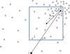 |
Fig. 1. Schematic 2D example of the lack of accuracy in the field computation caused by a large offset ΔCM. The center of gravity is far away from the ith particle, and the cube is not opened. Nevertheless, some particles that lie near the edge of the box, such as the jth and the kth points, are very close to the ith point, but their direct contribution is missed, which results in a loss of accuracy. |
We can furthermore optionally modify the opening criterion in our code by taking the offset term into account. We may use the following rule to open a box:
 (21)
(21)
This prescription is equivalent to the classic opening criterion, but with an effective opening angle θ′< θ, to guarantee that every close box is opened. In some peculiar cases in which ΔCM is large (i.e., comparable with the length of the semidiagonal of the box), as in the example of Fig. 1, the effective opening angle is considerably smaller than θ. In Sect. 3.2 we show that for a typical value of θ = 0.6, the adoption of the new criterion does not require too much additional computational effort, especially when many particles are involved.
3. Code testing
We illustrate here some basic physics tests (Sect. 3.1) and a series of performance tests (Sect. 3.2). In Sect. 3.1 we apply GaSPH to two basic problems: (i) a non-hydrodynamical system, characterized by a cluster of point-mass particles distributed according to a Plummer profile, and (ii) a classical shock-wave problem. These quality tests are followed by some applications to hydrodynamical systems at equilibrium. First, we treat some polytropes with finite radius. Then, we compare our algorithm with a well-known hydrodynamical tree-based code (Gadget-2) in the case of a gaseous Plummer sphere. In Sect. 3.2 we analyze the computational efficiency and the accuracy of our code in different contexts.
3.1. Tests with gas and pressureless systems
3.1.1. Turning off the SPH: the evolution of a pressureless system
In order to test the stability of our numerical method, we performed a series of simulations in which we placed a set of points according to the standard Plummer configuration (Plummer 1911), which is often adopted to study the distribution of stars in globular clusters. The Plummer sphere is pressureless, so that the particles interact only though gravity, and there is no SPH interaction. As units of measurement, we chose the total mass M and the gravitational constant G, and we placed an ensemble of N = 105 particles in a Plummer distribution with core radius R = 1 and cutoff radius Rout = 10R. The particles had equal masses m = N−1 and equal softening length ϵ, chosen as a fraction of the central mean interparticle distance:  (with αs ∈ [0.2, 1.0]). Starting the Plummer distribution at the virial equilibrium, we integrated its time evolution for 50 mean crossing-times τc. This parameter is defined as the initial ratio between the half-mass radius and the mean dispersion velocity
  . Figure 2 shows the virial ratio
  as a function of time and compares four runs made with different combinations of the opening angle θ (0.6; 1.0) and ϵ (0.2; 0.5). The four results illustrated in Fig. 2 do not show any relevant difference: the virial ratios oscillate within a small fraction < 0.5%, especially for the configuration with θ = 1 and αs = 0.5, which was expected to be the worst case.
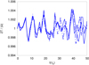 |
Fig. 2. Oscillation of the virial ratio as a function of time for different choices of code configuration parameters for the simulation of a Plummer distribution of 105 equal-mass particles. The continuous line shows θ = 0.6, ϵ = 0.2; the dashed line represents θ = 1.0, ϵ = 0.2; the dotted line shows θ = 0.6, ϵ = 0.5; and the dash-dotted line denotes θ = 1.0, ϵ = 0.5. |
We note that we do not work with a classical high-precision N-body code such as Nbody-6 (for example see Aarseth 1999). The Newtonian force is approximated by means of both the multipolar expansion, which occurs when particles are sufficiently far, and the softening length damping, which occurs when the particles approach within a distance of about ϵ. Despite these approximations, acceptable results can be obtained in a noncollisional system like our Plummer distribution. The results lie within reasonable errors.
3.1.2. Sedov–Taylor blast wave
To test the code with strong shock waves, we simulated the effects of a point explosion on a homogeneous infinite hydrodynamical medium with constant density ρ0 and null pressure. If an amount of energy E0 is injected at a certain point r0, an explosion occurs and then a radial symmetric shock wave propagates outward. Sedov (1959) investigated this problem and found a simple analytical law for the time evolution of the shock front:
 (22)
(22)
where rs is the radial position of the front relative to the point of the explosion r0, while a is a function of the adiabatic constant γ (it is close to 0.5 for γ = 5/3, and it approaches 1 for γ = 7/5). Furthermore, the fluid density immediately behind the shock front (r ≤ rs) has the following radial profile:
 (23)
(23)
where Gγ is an analytical function of the relative radial coordinate r/rs. Similarly as in many previous works (see, e.g., Rosswog & Price 2007; Tasker et al. 2008), we set the initial conditions for a homogeneous and static medium (ρ0 = 1, v = 0) by placing 106 equal-mass particles in a cubic lattice structure, confined in a box with x, y, and z coordinates each ranging from −1 to 1. γ was set to 5/3, and the explosion was simulated by giving an amount of energy E0 = 1 to the origin of the system. We were unable to reproduce a point explosion with an SPH system because its spatial resolution is determined by the kernel support. We therefore needed to inject the energy in a small region with the same scale as 2h. We thus gave at a time t* the energy E0 to the particles that were enclosed in a sphere with radius R = 2h. Figure 3 shows three different radial average density profiles ρ(r, t′) that correspond to the times t = 0.05, t = 0.1, and t = 0.2. The results are compared with the analytical solution. Although the position of the front follows the expected law of Eq. (22), the peak does not reach the expected value  .
.
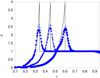 |
Fig. 3. Radial density profiles of the Sedov–Taylor blast wave at several times (increasing rightward) t = 0.05 (circles), t = 0.1 (triangles), and t = 0.2 (squares) in a simulation with N = 106. The results obtained using a higher resolution (N = 3 375 000) are plotted with dotted lines. The full lines represent the classical Sedov–Taylor auto-similar solutions. |
Intrinsic errors in approximating the physical quantities, given by the smoothing kernel, allow the density to spread out and follow a wider distribution than the true profile. This corresponds to a smoothing of the vertical discontinuity and so to a lower peak of the density. The same figure shows a comparison with results obtained from a further test that was made with the same system, but using a better resolution (N = 3 375 000). The peak of the curve clearly reaches a higher value.
3.1.3. Polytropes at equilibrium
We tested our code in the case of hydrodynamic self-gravitational systems by building static polytropes with different indexes (n = 1, n = 3/2, and n = 2). A generic polytrope of index n constitutes a radially symmetric system whose equation of state follows the expression
 (24)
(24)
where the density is parametrized as ρ(r)/ρ0 = θn(r), and ρ0 is the central value. The static radial solution θ(r) can be found by writing an equilibrium condition between the hydrostatic pressure gradient and the gravitational forces, from which the well-known Lane–Emden equation can be obtained (an exhaustive treatment can be found, e.g., in Chandrasekhar 1958):
 (25)
(25)
with  , and Kn a suitable normalization coefficient. For an index n ∈ (0, 5), the system has a finite radius and the coefficient Kn depends, through α2, both on the radius R and on the total mass M. We set both of them to 1 in our tests, implying K1 ≈ 0.637, K3/2 ≈ 0.424 and K2 ≈ 0.365.
We tested the ability of our code to let a system spontaneously relax in a polytrope configuration, following the prescription adopted in Price & Monaghan (2007). Starting from a homogeneous sphere of particles placed in a lattice structure, the system was let evolve by forcing the pressure to follow Eq. (24). We forced the SPH system to evolve by damping the velocities with an additional acceleration adamp = −0.05 v, until the kinetic energy decreased to a small fraction (1%) of the total energy. A standard nonconstant α was chosen for the artificial SPH viscosity, with α0 = 0.1, and a number of neighbors of 110 was set for the particles.
A correct treatment of self-gravity and hydrodynamic interactions among SPH particles, and the choice of the equation of state (24) allows the system to acquire the density profile ρ0θn, which is the solution of Eq. (25). Figure 4 shows the three radial density profiles we obtained for the different polytropic indexes. The resolution, related to the particles number, affects the accuracy of the code in correctly sampling the profile ρ(r), especially in the central denser regions. Mainly for the higher index n = 2, a higher particle number is needed to let the numerical density approach the theoretical expected value at a specific accuracy level. 10 000 particles were used for the models with n = 1 and n = 3/2, while the polytrope with index n = 2 was built with 20 000 particles.
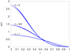 |
Fig. 4. Equilibrium analytical solutions of the density profiles ρ(r) related to three different models of polytropes with indexes n = 1, n = 3/2, and n = 2, drawn as solid curves. Comparison with the computed profiles (dots). |
3.1.4. Gaseous Plummer distribution
We tested the equilibrium of a static gas density distribution according to the Plummer function:
![Mathematical equation: $$ \begin{aligned} \rho (r) = \rho _0 \left[ 1 + \left( \dfrac{r}{a} \right)^2 \right]^{-5/2} , \end{aligned} $$](/articles/aa/full_html/2019/08/aa33143-18/aa33143-18-eq50.gif) (26)
(26)
with the central density defined by ρ0 = 3M/4πa3, where M and a are the total mass of the system and a characteristic length, respectively. We set M = 1 and a = 1 (G = 1 in internal code units) so that the half-mass radius of the system is r(50%) ≈ 1.3. In a static configuration with a null velocity field, the gas SPH particles compensate for the mutual self-gravity with a pressure gradient that results from a temperature distribution T(r)=κρ(r)1/5. κ represents a constant that is calibrated by taking the equation state of a perfect gas P = (γ − 1)ρu into account and by imposing the virial equilibrium between gravitational energy W and total thermal energy  , that is, |W|=2U. We placed 50 000 particles according to a Monte Carlo sampling of the distribution in Eq. (26). A realistic distribution has an infinite radius, therefore we used a cutoff at a proper radial distance r ≈ 22, such that the distribution contained 99.8 % of the mass of a realistic infinitely extended Plummer sphere. Figure 5 shows the time variation of some Lagrangian radii that contain 5%, 15%, 30%, 50%, 75%, and 90% of the total system mass for an integration time of 90 central free-fall timescales ( τ0 = (3π / 32Gρ0)1/2 ≈ 1 in our code units).
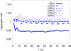 |
Fig. 5. Lagrangian radii as a function of time for a hydro-Plummer distribution at equilibrium (see Sect. 3.1.4). The radii are normalized to their respective initial values. |
We compared the results with the well-known gravitational SPH code Gadget-2 (Springel 2005). Figures 6 and 7 show a comparison between the radial density profiles obtained by the two algorithms with the same choice of the main parameters. The α viscosity coefficient was set constant and equal to 1. The reported density was computed at t = 90 τ0, even though the system reached an acceptable equilibrium state already within a few units of τ0 after several slight oscillations.
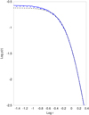 |
Fig. 6. Radial density profile for a Plummer distribution with 50 000 SPH particles (solid line). The results obtained with Gadget-2 are also shown (dashed line). The analytical Plummer profile is plotted with a dotted line. The density is in units such that ρ0 = 3/(4π). |
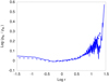 |
Fig. 7. Logarithmic ratio ρN/ρA of the numerical to analytical radial density profile for a Plummer distribution with 50 000 SPH particles (solid line). The results obtained with Gadget-2 are also shown (dashed line). |
In Fig. 7 we can distinguish three main radial zones for r ≤ 0.3, 0.3 < r < 2, and r ≥ 2. In the middle zone, the codes are in good agreement and provide a density profile with an accuracy lower than 2% with respect to the analytical model. For r < 0.3, Gadget-2 describes a density that deviates by up to the 6% from the expected value, while our program has a maximum deviation of 11%. For both models, these higher errors can be ascribed to the fact that the system contains only about 2% of the total mass (and thus 2% of the total particles) within the radial distance r = 0.3, which causes a poor sampling of the potential inside the sphere. Consequently, the system tends to shrink slightly. In the outward zone, the deviations can reach significantly higher values with both codes because the density values are far lower than in the central zone. We therefore conclude that in the context of a standard physical environment, the two codes show a satisfactory agreement overall.
3.1.5. Artificial viscosity and angular momentum conservation
A nonconstant artificial viscosity may lead to nonconservation of the angular momentum, L. The actual conservation of this quantity was tested with different settings of the artificial viscosity parameters in Eq. (14), integrating the time evolution of a system that was very similar to the one described in the previous section. We used the same Plummer distribution (see Eq. (26)), with M = 1 and a = 1, made of 50 000 SPH particles. The same thermal energy profile was adopted, but scaled down by a factor 1/2, so that 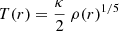 . We converted the (subtracted) thermal energy into kinetic energy by assigning to each ith particle a clockwise azimuthal velocity, with absolute value
  (where ui was the original specific thermal energy characterizing the Plummer system used in Sect. 3.1.4), and a direction parallel to the X, Y plane. The system thus acquired a nonzero vertical component of the angular momentum,
 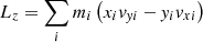 . The virial equilibrium was still formally preserved because gravitational potential energy and thermokinetic energy were the same such that |W|=2(K + U), but the (new) angular rotation triggered changes in the density distribution. We integrated in time for about 100 initial central free-fall timescales τ0 (which is on the same order as the azimuthal dynamical timescale, taken as the ratio rc/v(rc)≈1.4, where rc is the initial radius at which the density drops by a factor 1/2). We performed three different simulations by varying in the α rate Eq. (14) the parameters αmin and b. We set αmin = 0.1, b−1 = 5, αmin = 0.02, b−1 = 5, and αmin = 0.1, b−1 = 7. The angular rotation changes the configuration of the system, which causes the initial Plummer density distribution to become flatter perpendicularly to the z-axis, while the whole system expands. During an initial phase of about 20τ0, the distribution underwent some rapid variation followed by a slow secular evolution. Figure 8 shows the quantity (Lz−Lz0)/|Lz0|, which represents the variation as a function of time of the component Lz compared to its initial value Lz0. The three lines refer to the different choices of the parameters αmin and b. The curves show a conservation of the angular momentum within 10−3 up to 100 evolution timescales. In particular, the choice of αmin = 0.1, b−1 = 7, compared with the other configurations, gives a stronger variation of Lz during the first phases, while it shows a lower change rate during the secular evolution of the system. On the other hand, a low value αmin = 0.02 gives rise to a better conservation in the initial phases and a higher deviation during later stages. We observed in all three simulations that the two components Lx and Ly maintain values compared to Lz within a relative error of 10−3.
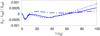 |
Fig. 8. Fractional variation in the z-component of the angular momentum for our simulated rotating Plummer model (see Sect. 3.1.5). We plot the results obtained by varying some configuration parameters: αmin = 0.1, b−1 = 5 (full line), αmin = 0.02, b−1 = 5 (dotted line), and αmin = 0.1, b−1 = 7 (dash-dotted line). |
3.2. Code performance
In order to analyze the computational efficiency of our algorithm as a function of the particle number, we performed several tests by measuring the average CPU time that was spent for a single run by the main routines. We therefore studied the performances of the GaSPH code in three different contexts:
-
(1)
A system with pure self-gravity and zero pressure, adding a comparison with the results of Gadget-2.
-
(2)
A system with self-gravity and SPH pressure.
-
(3)
A system similar to that of case 2, but with the addition of 20 point star-like external objects.
We performed the tests by placing a set of N particles with the same Plummer density profile distribution as adopted in Sect. 3.1.1. The program was tested on an Intel®CoreTM i7-4710HQ architecture with 6MB of cache memory and with 16GB of RAM memory DDR3L with a data-transferring speed of 1600 MHz.
For a standard tree code without SPH, the computational time per particle is expected to be linear in log N because the overall time scales as N log N. To increase the efficiency and save considerable memory resources, we can also use a simple formalism made by considering only the first “monopole” term −MGr−3r that appears in the right member of Eq. (3). This is a technique that was also adopted in Gadget-2 and simplifies the complexity of the algorithm by neglecting the efforts for the quadrupole tensor computation. The suppression of the quadrupole term decreases the computational time, with a minor cost in terms of accuracy. For a pure self-gravitating system, Fig. 9 shows the CPU time needed for a single particle force calculation as a function of the ten-based logarithm of the particle number N (ranging from 104 to 5 × 10⁶). Choosing an opening angle θ = 0.6, we performed a series of force evaluation by considering a simple pressureless system, with particles interacting only with the Newtonian field. The computational times measured using our code (averaged over a reasonable number ≥30 of equal tests) are comparable with the average CPU times measured using Gadget-2. The figure also shows the results based on a second series of runs with GaSPH performed with the quadrupole term included in the gravitational field. Including this term, an additional CPU time of about 30% is requested. Figure 10 compares the previous CPU times with the times needed by GaSPH for a full self-gravitating SPH system, with the quadrupole term included in the computation and the same value of θ = 0.6. The times per particle for the density computation routine are also shown. In computing the acceleration, the additional time per particle is fairly independent of N, as can be seen in the figure, because the close SPH interactions are always made over a fixed number of neighboring points, which we set to 60 in this example. For the same reasons, the average time per particle needed to calculate the density is also expected to be constant, as Fig. 10 shows. The calculus of ρ and h requests an iterative process in which the routine for each particle is called several times. The CPU times illustrated in the figure are the average values per single iteration. Determining the optimum value of h the code typically requires no more than two iterations.
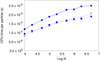 |
Fig. 9. CPU time per particle for the pure gravitational force calculation in monopole and quardupole approximations at different N. Gadget-2 results (empty circles) are compared to our code results (squares connected with dashed lines) in the same monopole approximation. The continuous line refers to the performance of GaSPH, and the quadrupole term is included in the field. |
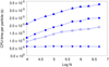 |
Fig. 10. GaSPH average CPU times per particle as a function of N. Comparison of different routines: SPH neighbor-search routine averaged for a single iteration (circles), pure gravity computation with monopole term (empty squares) and with quadrupole term (filled squares), self-gravity computation up to quadrupole and including the SPH terms (triangles). The units are the same as in Fig. 9. |
The optional introduction of the offset ΔCM term in the opening criterion (as discussed in Sect. 2.2.6) causes in some cases a considerable reduction of the effective angle θ. Consequently, the number of direct particle-to-particle interactions increases, which decreases the code performance. Figure 11 illustrates the code efficiency in terms of number of particles processed in a second. The results, related to the two acceleration routines (pure self-gravity and self-gravity with SPH) shown in the previous graph, are compared with other result obtained by including the offset term ΔCM in the opening criterion of Eq. (21). A substantial but not drastic worsening in performance can be observed. For instance, using 5 × 10⁶ SPH particles and including ΔCM, the code computes the accelerations at a rate of ≈24 000 particles per second (about 17% slower than the case without ΔCM). Computations were made with θ = 0.6 and including the quadrupole terms. The performance of the same two force subroutines (pure gravity and gravity plus hydrodynamics) were also studied at different values of θ (CPU times per particle as a function of N are shown in Fig. 12).
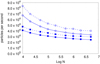 |
Fig. 11. Number of processed particles per second. The continuous lines and the dashed lines refer to results with and without the correction term ΔCM, respectively. We show the simple gravity field calculation (empty circles) and the full self-gravity routine with hydrodynamics (squares). The quadrupole term is considered for the gravity field. θ = 0.6. |
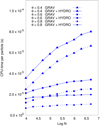 |
Fig. 12. Computational time per particle vs. log N for various values of the opening angle θ. The pure tree gravitational algorithm (dashed line) and full SPH+gravity algorithm are shown as dashed and solid lines, respectively. The quadrupole term is included in the force evaluation. The ΔrCM offset term is not considered by the opening criterion. |
Smaller angles should provide higher precision at the cost of a longer computational time. On the other hand, with larger angles there are fewer direct point-to-point interactions and we gain in efficiency, but we expect a lower accuracy. We evaluated the accuracy of our tree code by measuring a “mean relative error” in computing the accelerations according to the prescription suggested by Hernquist (1987), with different conditions of particle number N and opening angle θ. The prescription consists of a comparison of the three components of the acceleration vector as computed by means of the tree scheme,  , with the “exact” value
  computed by direct summation. A mean error
  is computed by averaging over all the N particles. Then, the relative error is computed as follows:
 (27)
(27)
Figure 13 shows these relative errors, obtained with GaSPH, as a function of the CPU time. The figure does not show the relative errors for each single component, but shows the mean values, computed by the simple average  . Results for several setup configurations are illustrated. The figure shows the results in three different panels, according to the value of N (N = 104, N = 105, and N = 106). For each value of N, we used different combinations of the parameter θ (0.4, 0.6, 0.8) with different opening criteria (Eq. (20) or Eq. (21)) and different multipole approximations (only the monopole term, or also including the quadrupole term). As the data show, the approximation of the field with the quadrupole moment always represents the best choice in terms of performance because at the same error, it requests a shorter CPU time than the monopole approximation. On the other hand, the choice of the new opening criterion gives a smaller improvement of the error with respect to the benefits that are obtained by switching from monopole to quadrupole term.
 |
Fig. 13. Tree code relative errors Err(ak) (averaged over all the three Cartesian coordinates) for the gravitational field computation as a function of the CPU time. The data are illustrated for different particle numbers (N = 104, N = 105, and N = 106) in panels a, b, and c. In each panel, the full line connects the points related to a computation of the gravitational field made with the quadrupole approximation, while the dashed line refers to computations made by using just the monopole term. The shape of the “void” markers distinguishes different choices of θ with the “standard” criterion (Eq. (20)): θ = 0.8 (void squares), θ = 0.6 (void triangles), and θ = 0.4 (void circles). Results for different opening angles with the “opening law” (Eq. (21)) criterion are also marked: θ = 0.8 (solid squares), θ = 0.6 (solid triangles), and θ = 0.4 (solid circles). |
For lower particle numbers, a better computational performance without loss of accuracy can be obtained by including the quadrupole approximation and the (more expensive) opening criterion given in Eq. (21), together with a suitable change of the θ angle. We focus, for example, on the simulation setups characterized by θ = 0.6 with any possible opening criterion, monopole approximation, and N = 104 or N = 105. The change θ = 0.6 → θ = 0.8, together with the use of criterion (21), represents a good choice and provides better performing simulations without degrading the precision of the algorithm. We obtain the same advantage when we pass, similarly, from θ = 0.4 to θ = 0.6. On the other hand, for N = 106 (panel c in Fig. 13), the results related to the approximation with monopole and with quadrupole have smaller differences than the other cases with different N. The choice of a larger opening angle (passing from θ = 0.6 to θ = 0.8 or passing from θ = 0.4 to θ = 0.6) together with the use of the new opening criterion can give a better performance even though the accuracy slightly decreases.
If we wish to preserve the high efficiency of the tree code by keeping the CPU time to scale as N log N, an angle θ ≥ 0.3 must be chosen (Hernquist 1987). The choice of θ = 0.6 in quadrupole approximation or the choice of θ = 0.4 in monopole approximation together with criterion (21) represents a satisfying option because it provides relative errors of at most about 10−3.
We now added Nob = 20 stars to the SPH distribution. As explained in the previous section, a 14th-order explicit method was applied to calculate the evolution of these objects, and giving their low number in comparison to N, very little additional CPU time is expected. Table 1 reports the percentage or workload related to the main relevant subroutines for the new gas+stars system: tree-building + particle-sorting routine, density computation routine, acceleration routine, and the star evolution routine. In addition, we report the rest of the time needed for the basic operations (such as v, u, and r updating, energy computation, and time-step computation). Different work balances are shown for several values of N. The percentage of workload related to the tree-building routine is stable to the order of 6% at different N. In contrast, the work needed by the density routine becomes less and less relevant as N increases, while the gravity+SPH computation becomes increasingly essential. The computational effort to treat the evolution of stars, together with their interaction with the gas, is due both to the pure N-body RK coupling, which is expected to scale as  , and to the time for coupling each star with each SPH particle, which is expected to be linear in N. Nevertheless, Table 1 shows that 20 stars contribute very little to the total CPU time. For the specific purposes of our current work, we used fewer than two stars or two stars, and their contribution to the code effort is therefore far lower than the 2%÷3%.
Work profiling (in percentage with respect to the total) of GaSPH, tested on a Plummer gas distribution with 20 stars and different numbers of SPH (first column).
4. Protoplanetary disks
This section is dedicated to the description of some tests performed on two main problems involving protoplanetary disks. The first test is to compare the numerical integration of a disk around one star with the analytical prediction (Sect. 4.1). The second test involves a self-gravitating disk that interacts with a binary star (Sect. 4.2).
4.1. Protoplanetary disks around one star
4.1.1. Disk model
Here we illustrate the general setup we used to model a protoplanetary disk in equilibrium around a star of mass Ms = 1 M⊙. According to the classical flared-disk model (see, e.g., Garcia 2011; Armitage 2011), we let the disk revolve around the central object with a roughly Keplerian frequency 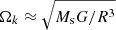 (where R is the cylindrical coordinate
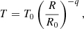
  in the reference frame centered on the central object). The disk evolution is essentially driven by secular viscous dissipation. According to the well-known α-disk model (Shakura & Sunyaev 1973), the turbulence in the internal disk is schematized by means of a pseudo-viscosity of the following form:
 (28)
(28)
This kinematic viscosity perturbs the fluid equations by leading to a net transport of matter inward and an outward flux of angular momentum. αSS represents a characteristic efficiency coefficient for the momentum transport, while H = cs/Ωk represents a characteristic vertical pressure of the disk scale height. The viscous evolution is usually much slower than the dynamical evolution (the characteristic secular timescale is ∝r2/ν, which typically is 2 or 3 orders of magnitude larger than  ). This modeling of the turbulence is basically dimensional and is made by mainly taking dynamical turbulence processes into account. Thus, αSS extends over a wide range of variability (typically 10−4 and 10−2). When the disk self-gravity is strong enough, another important effect arises that is due to the gravitational perturbations. Several works (see, e.g., Mayer et al. 2002; Boss 1998, 2003) have numerically estimated the gravitational timescales in a protoplanetary disk, which is on the same order as its dynamical time. They showed that under certain conditions, matter can undergo instabilities and eventually condense to form clumps in 103 ÷ 104 yr, which may give rise to gaseous planets. It can been shown that the disks maintain their equilibrium state against collapse according to the Toomre criterion,
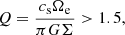
 (29)
(29)
where Ωe represents the epicyclic frequency, which is approximatively equivalent to Ωk for Keplerian disks (see Binney & Tremaine 1987; Toomre 1964, for a detailed study). The Toomre factor is a general coefficient that quantifies the predominance of the gravitational processes over the typical thermal and dynamical actions.
We initially let our disk revolve with an azimuthal velocity 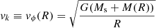 that depends both on the mass of the central star Ms and on the internal mass of the disk itself
 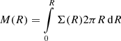 . The cumulative mass M(R) can be neglected only for low disk masses MD ≪ Ms. The shape of the disk in the direction perpendicular to the revolving midplane depends on the vertical pressure scale height H, such that pressure and density scale with a Gaussian profile exp(−z2/2H2). Here a local vertically isothermal approximation was used because we assumed that any radiative input energy from the star is efficiently dissipated away: the cooling times are far shorter than the dynamical timescales. The disk is thus vertically isothermal, and the temperature depends only on the radial distance from the central star.
We set the thermal disk profile according to the well-known flared-disk model, for which the ratio H/R increases with R (see Garcia 2011; Dullemond et al. 2007, for a full clarification). The disk temperature thus follows the profile
 (30)
(30)
which is commonly used by setting q = 1/2, while R0 represents a scale length. We used a slightly different slope q = 3/7, adopted by D’Alessio et al. (1999) by assuming that the thermal processes in the inner layers of the disk do not affect its dynamical stability.
With this temperature profile (independent of t and z), the gas pressure follows a barotropic equation of state  . This choice represents a rough approximation of the cooling processes and allows us to model self-gravitating disks in equilibrium only when Q > 2, which excludes disk models with a state of marginal stability (Q ≈ 1). In a realistic model of a disk without the isothermal approximation, when the Toomre parameter approaches unity, the loss of thermal energy due to radiative cooling processes leads to matter aggregation, which in turn causes shock waves that heat the gas again. If the disk is capable of retaining a sufficient amount of the additional thermal energy that is generated, the collapse only causes some spiral instabilities that do not increase exponentially. The collapse process is thus arrested and the disk reaches a meta-stable state. Every time that a gravitational instability occurs, it is further dissipated by the heat back-production in this meta-state. For a good treatment, see for example Kratter & Lodato (2016). Conversely, the isothermal equation adopted by our model forces the system to cool down at an infinitely high efficiency rate, and to expel all the additional thermal energy that is generated by the compression of matter. Thus, in regions where 1 ≤ Q < 2, the density increases and the collapse process is not halted by production of heat. Our model of a disk in equilibrium is thus limited to masses MD for which the self-gravity guarantees the condition Q ≥ 2.
We used  as the mean molecular weight for the gas. This parameter is commonly adopted to model protoplanetary disks (see, e.g., Kratter et al. 2008; Liu et al. 2017) because it is an average mean weight for a gas composed of H2 and He, based on the observed cosmic abundance of the elements.
The effects of the Shakura-Sunyaev viscosity associated with Keplerian disks can be emulated by means of the SPH artificial viscosity. Meglicki et al. (1993) found that the SPH viscosity coefficient α provides a viscous acceleration with an effective kinematic viscosity that contains a similar form with a shear component plus a bulk viscosity. When a cubic spline function is used for the kernel function, the authors showed that ν assumes the following form:
 (31)
(31)
In several works (e.g., Artymowicz & Lubow 1994; Nelson et al. 1998) the viscosity term in Eq. (11) is used under peculiar conditions: it acts not only for approaching particles, but also for points that move out (with rij ⋅ vij > 0). It turns out that ν = 0.1 αcsh (for a comprehensive explanation, see Meru & Bate 2012). We thus have the following law that connects the Shakura–Sunyaev viscosity coefficient to the α parameter used in SPH:
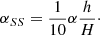 (32)
(32)
This modification of the SPH formalism provides a more realistic prediction of the effect given by a kinematic viscosity because it acts under compression and under gas expansion. This prescription is reliable except for strong velocity gradients, that is, shock waves due to strong compressions. In this case, the classical Morris & Monaghan (1997) amplification law (Eq. (14) in this paper) would generate high dissipative forces even in expansion regions. Protoplanetary disks are usually modeled as quiet systems and are not expected to undergo such huge compressions to let strong shock waves arise.
Using Eq. (11) for the viscosity, and consequently, activating dissipation only for particles approaching each other, the law in Eq. (32) can be modified and improved by also considering the effects of the β coefficient on the kinematic viscosity (Meru & Bate 2012; Picogna & Marzari 2013). It follows that for Keplerian disks,
 (33)
(33)
Equations (32) and (33) formally do not contain any effect of the Balsara switch to compensate for the false sharing attenuation (Eq. (12)). As was done in Picogna & Marzari (2013), we used the artificial viscosity term of the disk in Eq. (11), and multiplied the factor μij by the term of Balsara (1995)
 .
.
4.1.2. Evolution of the viscous disk
We tested the response of our model with respect to dissipative processes with long timescales as are characteristic of viscous turbulent disks. We started from the well-known disk model developed by Lynden-Bell & Pringle (1974) (see also Pringle 1981; Hartmann et al. 1998). It consists of a thin (H/R ≪ 1) non-self-gravitating disk that is subjected to a power-law dissipative turbulent viscosity. The surface density evolution is described by the following equation (see Pringle 1981; Hartmann et al. 1998):
![Mathematical equation: $$ \begin{aligned} \dfrac{\partial \Sigma (R,t)}{\partial t} = \dfrac{3}{R}~ \dfrac{\partial }{\partial R} ~ { \left[ ~ R^{1/2} \dfrac{\partial }{\partial R} \left( R^{1/2}~ \nu ~\Sigma (R,t) \right) ~ \right]} . \end{aligned} $$](/articles/aa/full_html/2019/08/aa33143-18/aa33143-18-eq75.gif) (34)
(34)
It has been shown that when the disk is perturbed by a radial power-scaling kinematic viscosity ν ∝ Rϕ, the differential equation admits the following similarity solution (see Lynden-Bell & Pringle 1974; Hartmann et al. 1998):
![Mathematical equation: $$ \begin{aligned} \Sigma (R,t) = \Sigma _0 \left(\dfrac{R}{R_1}\right)^{-\phi } \left( \dfrac{t}{\tau _\nu } + 1 \right)^{-\gamma } \exp \left[-\left( \dfrac{t}{\tau _\nu } + 1 \right)^{-1}\left(\dfrac{R}{R_1}\right)^{2-\phi } \right], \end{aligned} $$](/articles/aa/full_html/2019/08/aa33143-18/aa33143-18-eq76.gif) (35)
(35)
where  . R1 is a characteristic radial scale that contains about the 68% of the total disk mass, while Σ0 is the normalization scale density. In Eq. (35),
  represents the characteristic viscous timescale of the disk, and it is proportional to the inverse of the viscosity evaluated in correspondence to the scale radius (ν1 = ν(R1)).
We sampled a disk, made of 20 000 particles, which followed the thermal law of Eq. (30) described in the previous section, where we assumed R0 = 10 AU for scaling and T0 = 25 K. The SPH particle distribution was achieved by sampling the initial (t = 0) radial density profile as from Eq. (35),
![Mathematical equation: $$ \begin{aligned} \Sigma (R,0) = \Sigma _0 \left(\dfrac{R}{R_1}\right)^{-\phi } \exp \left[-\left(\dfrac{R}{R_1}\right)^{2-\phi } \right], \end{aligned} $$](/articles/aa/full_html/2019/08/aa33143-18/aa33143-18-eq79.gif) (36)
(36)
where R1 was set here to 50 AU. We used a constant value for the viscosity coefficient, αSS = 10−2. The kinematic viscosity is proportional to the sound speed and the vertical scale height (Eq. (28)), and when we assume that the exponent q = 3/7 in the power-law Eq. (30), ν follows a radial power law with a positive exponent ϕ = 15/14 ≈ 1.07. In order to reproduce the effects of such a radial viscosity law, we imposed a specific prescription for the artificial viscosity in the code. Taking the law of Eq. (33) into account and considering that we used β = 2α, we obtain the following expression for the coefficient α:
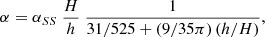 (37)
(37)
with constant αSS = 10−2. To apply this form, we inserted the expression above in the artificial viscosity term of Eq. (11), which we used in all our disk simulations, without considering the Morris & Monaghan (1997) variation law.
The (infinite) disk has been truncated at Rout = 8R1 = 400 AU. The distribution was also truncated at an inner cutoff Rin = R1/5 = 10 AU. The gravitational softening radius of the central star together with its sink radius were set equal to Rin. The inner border condition we set is that the gas particles that cross the Rin radius are absorbed by the star and are therefore excluded from time integration. The mass of the sunk SPH particles was considered to increase the mass of the central star.
The ratio Rout/Rin ≈ 40 is high enough to match the infinite extension of the analytical density profile as accurately as possible. This reduces the external radial boundary discontinuity. Hartmann et al. (1998) indeed pointed out that the inward flux of matter (which constitutes the most important process in guiding the evolution of an α disk) considerably depends on the outward angular momentum transportation and thus on the disk expansion through the external shells.
The boundary conditions at Rin > 0 may affect the disk evolution throughout the whole spatial extension. As pointed out in Lynden-Bell & Pringle (1974) and remarked by Hartmann et al. (1998), a viscous disk may formally extend to R → 0, but at a critical radius that is on the same order as the radius of the star, both the torque and the viscosity ν go to zero. Computational efficiency purposes prevent us from modeling a disk by introducing a very small cutoff radius. We imposed zero viscosity ν by varying the coefficient α within R = 3Rin down to zero, assumed at R = Rin.
Parameter α in Eq. (37) varies with time because the disk evolution processes lead to a time variation of the ratio between h and the height scale H. For R = R1/2 the disk initially has an average h/H ≈ 2, while this ratio reaches a minimum value of about 1.5, in correspondence to R = 2R1, which provides a value of α ≈ 0.02 and α ≈ 0.04, respectively. As the gas is captured by the central star, we expect the density to decrease and the h-to-H ratio to increase. We show below that the surface density varies quickly during an initial phase and later evolves at a relatively lower rate; this causes h/H to follow the same cadence. At later stages (after about 1.6 Myr), the disk is indeed integrated with lower values of α that range from approximately 0.01 to 0.03.
Our disk is virtually non-selfgravitating because Q ≫ 2 throughout its surface (the minimum value is about 20), even though we formally took the disk mass into account in setting the azimuthal velocity vϕ(R). For R = R1, it has a vertical aspect ratio H/R ≈ 0.05. With this setup, the disk should have a viscous evolution timescale τν ≈ 840 000 yr according to the analytical model.
During the earlier integration phases, the disk experiences a fast relaxation caused by the inner cutoff. In this stage the internal density discontinuity is smoothed out and fades out near the inner border. We therefore allowed the system to relax for a time of about 50 000 yr (about 900 Keplerian orbits at R = R1), which is far shorter than τν and sufficient to obtain a steady state. From this time, the only expected changes in the disk density profile are those that are due to the secular viscous evolution. Thus, after 50 000 yr, the disk is quickly arranged in a configuration that is slightly different from the initial one: it is characterized by a density distribution that follows the density law of Eq. (36), but now with a larger radius R1 ≈ 60 AU. With this new radius, the disk has an evolution timescale τν ≈ 106 yr. The properties of self-similarity according to Eq. (35) indeed guarantee that the surface density profile maintains the same analytical form for every time. Thus, the surface density of a disk can at every time be considered an initial solution of a new disk that is described by Eq. (36), with a different parameter R1 and thus a different viscosity timescale τν. The initial profile and the density profile after 50 000 yr (which we set conventionally as the instant t = 0) are shown in the top panel of Fig. 15. The initial t = 0 state fits (full line) the disk profile of Eq. (36) with R1 ≈ 60 AU. We considered the disk evolution to start from this configuration and plot the density profile for various times (t = τν/3 ≃ 330 000 yr and t ≃ 1 000 000 yr). We also compare this with the analytical predictions obtained by Eq. (35) (dashed lines). Results and model do not match because the numerical disk appears to evolve faster than the disk predicted by the analytical theory. For t ≃ 330 000 yr the discrepancy between the analytical density was about 45% higher than the numerical result at R = R1, while for t ≃ 1 000 000 yr the discrepancy increased up to 95%. The disk thus looses mass more quickly than would be expected based on analytical theory, and thus its density decreases too rapidly. This excessive loss can be ascribed to the inner border, which is absent in the analytical theory, where the disk matter flows onto the star in a single point. To check how incorrectly the SPH disk depleted its mass, we considered the radial-cumulative disk mass, predicted at a given time by the analytical theory, which is strictly connected to the viscosity timescale,
![Mathematical equation: $$ \begin{aligned} M(\le R,t) = M_{\rm D}(0) \left( \dfrac{t}{\tau _\nu } + 1\right)^{\frac{-1}{2(2-\phi )}}\left[1 - \exp \left( \left(\dfrac{R}{R_1}\right)^{2-\phi }\left( \dfrac{t}{\tau _\nu } + 1\right)^{-1}\right)\right] , \end{aligned} $$](/articles/aa/full_html/2019/08/aa33143-18/aa33143-18-eq81.gif) (38)
(38)
where MD(0) is the starting disk mass at t = 0. In Fig. 15 we illustrate the fractional disk mass-loss rate  as a function of time. The result obtained with our model is compared with the theoretical rate, where the mass as a function of time was considered as the integral of the analytical surface density in Eq. (35), from R = 10 AU and R = ∞, that is,
  , where MD(t) is the total disk mass at a given time. The SPH-disk mass-loss rate tends to reach the analytical curve only for t → τν), while for earlier stages, we have a huge mass-loss rate that decreases as time approaches τν.
To make a more substantial comparison, we moved out from the early stages and focused on the later phases at t′=850 000, where the mass-loss rate illustrated in Fig. 15 approached the analytic value to within 10%. For this time, we considered our model density distribution as the starting state of a new disk and studied its subsequent evolution. We summarize this evolution in Fig. 16. The figure shows that at t′, the disk density surface corresponds to a Lynden-Bell solution of the same form as the starting one, but with a different characteristic radius  . This radius corresponds to a viscous timescale
  yr. In the same figure we show the evolution of the new surface density after a time of
 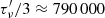 yr, together with the theoretically expected value (dashed line). This was made by analogy with Fig. 14, where the result at t = τν/3 ≈ 330 000 yr is shown (plotted in the middle). Comparing the two curves, we note that during the later stages the density of the SPH disk shows less deviation from the analytical prediction (within an error of 20% at
  ), although the discrepancies are not negligible. The discrepancies are also smaller in internal regions at
  , close to the inner border. To relate the discrepancy between the numerical density and its analytical prediction, we further verified this by adopting a smaller inner border radius, that is, by reducing the star sink from 10 AU to 5 AU, and we indeed observed a substantial reduction of the inner mass-loss rate of the disk in the initial integration phases. We also note that the gap of the surface density within the star sink radius is reduced in amplitude when a smaller inner boundary is chosen.
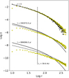 |
Fig. 14. Surface density profiles Σ(R) of the disk at different times (t = 0 corresponds to the disk state after it has been relaxed up to a time of 50 000 yr). The dots represent the numerical results, while the lines refer to the analytical model (Eq. (35)). The actual initial disk setting (black triangles) is reported for the sake of comparison with the relaxed state. The abscissa is in AU and the density is expressed in 10−2 M⊙ AU−2. The evolved density profiles at t > 0 (t = 330 000 yr and t = 1 000 000 yr) are shifted down by −3 and −6 in logarithm, respectively, for clarity. The fitting curve of the density profile at t = 0 is also plotted (full lines). |
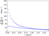 |
Fig. 15. Relative (percentage) mass-loss rate of the disk |

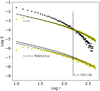 |
Fig. 16. Logarithm of the numerical radial profile of the disk density at t′=850 000 yr (dots). The density profile at the beginning of the simulation is also plotted (black triangles). The density at t = t′ matches the self-similar solution (Eq. (36)) with a parameter |


4.2. Self-gravitating disk in a binary system
We tested our code on a more complex dynamical system by treating the evolution of a self-gravitating disk that interacts with a binary star. The system is characterized by a circumprimary disk around a 1 M⊙ star, truncated by the gravitational field of a 0.4 M⊙ external companion star. This topic has been treated in a relevant work by Marzari et al. (2009), who integrated the time evolution of this configuration and studied the effects of the stars on the parameters of the orbital disk: eccentricity and argument of periastron. The authors used the well-known Eulerian code FARGO, implemented with a full scheme for the self-gravity (see Masset 2000; Baruteau & Masset 2008), and performed a 2D simulation. We investigated the evolution of a system like this with GaSPH with a 3D model for the particular case of a binary with eccentricity 0.4.
4.2.1. System setup
The orbit of the binary system is characterized by an eccentricity eb = 0.4 and a semimajor axis of 30 AU. As in Marzari et al. (2009), we kept the orbit of the two stars fixed during the integration because we focus on the gravitational effects of the two stars on the disk. This means that the dynamics of the binary star is not affected by the gas feedback. The initial configuration of the disk that was adopted in the original model is characterized by a radial surface density Σ ∝ R−1/2 that extended from 0.5 AU to 11 AU from the central primary star. Beyond 11 AU, the density quickly fades out; the total disk mass is MD = 0.04 M⊙. Instead of using a typical flared disk, we adopted a flat disk by setting the linear vertical scale height to H = 0.05 R.
The choice adopted by Marzari et al. (2009) for the disk shape and the viscosity law leads to a slightly different schematization than in the model we used in Sect. 4.1.2, for which we needed to set the parameters inside our SPH 3D code. The authors used a constant kinematic viscosity ν, which leads αSS to vary. Furthermore, the constant value of the aspect ratio H/R causes the speed of sound to scale as cs ∝ R−1/2. When ν = cost. and given the alpha-disk law of Eq. (28), we have that  . The coefficient αSS was indeed set by the above authors by calibrating it to correspond to the value αSS = 2.5 × 10⁻³ in the central regions about 5 AU within the disk. Thus, we can deduce it as follows:
 (39)
(39)
with Rref = 5 AU. We applied the artificial viscosity term by setting the SPH α parameter according to the same expression of Eq. (37) as we used in the previous section, but now using the nonconstant coefficient αSS with the radial profile of Eq. (39) illustrated above.
The disk is coplanar with the star orbit, and we built it by confining a set of SPH particles between R = 0.5 AU and R = 11 AU. We integrated the system for about 3000 yr. All the gas particles that flew across the inner border were excluded from the integration. Three runs for the same model were made with different particle numbers, N = 20 000, N = 50 000, and N = 100 000.
As in the case of protoplanetary disk around one star we discussed in the previous section, the ratio h/H, and consequently α, are not constant in time. For N = 20 000, the disk acquires a steady state configuration after an initial quick relaxation phase, where h/H has a rather slow evolution along the timescale of a binary rotation period. After about 500 yr, the disk acquires an average ratio h/H ≈ 6.5 (α ≈ 0.001) in the inner regions (R = 1 AU), which reaches a minimum of about 1 (α ≈ 0.011) in the middle regions (R = 5.5 AU). Similarly, the disk with N = 50 000 has an average ratio h/H ≈ 3.7 in the inner regions, with a minimum of h/H ≈ 0.7, corresponding to α ≈ 0.004 and α ≈ 0.02. The disk with N = 100 000 has α ≈ 0.008 in the internal regions and a maximum α ≈ 0.03 in the intermediate radial regions. Regardless of the resolution, after an integration time of 3000 yr, the h-to-H ratio slightly changes in the inner regions while its minimum substantially increases, giving rise to a maximum value of α of about 0.008, 0.015, and 0.02 for the disk with the lower, medium, and higher particle numbers, respectively.
4.2.2. Disk deformation and gravitational feedback to the stars
The gravitational field of the stars affects the disk configuration by altering its average orbital parameters such as the eccentricity and the argument of periastron. In order to describe the disk evolution, we calculated the mean eccentricity and the mean argument of periastron by averaging over the disk surface, with the same prescription as was adopted by Pierens & Nelson (2007),
 (40)
(40)
Here MD is the disk mass included within RA and RB (the latter being a quantity on the order of the effective radius RD). The disk radius is defined by the following expression:
 (41)
(41)
and is computed as the radial distance containing the total angular momentum L of the disk, with MD its total mass. RD is not very different from the half-mass radius.
The local orbital parameters are evaluated using the eccentricity vector,
 (42)
(42)
where l = rxv represents the angular momentum per unit mass, and Mc is the mass of the central star. The vector e characterizes the orbit described by the position r of a point about the center of mass of the binary, assuming that it corresponds to an elliptical trajectory. The absolute value e = |e| corresponds to the orbital eccentricity. Moreover, e is always parallel to the semimajor axis, thus, its normalized components ex/e = cos(ω) and ey/e = sin(ω) provide the local argument of periastron ω, and finally, the local semimajor axis. In Eq. (40), only the particles on orbits that are tied to the central primary star are considered part of the disk and thus are included in the summation.
The choice of a 3D model introduces some new degrees of freedom with respect to a 2D scheme because the self-gravity of the disk and the gravity of the stars act even along the vertical direction. In particular, the angular momentum, whose flux across the disk plays a crucial role on the disk evolution itself, is also spread out in the vertical direction.
Figures 17 and 18 show the evolution of the disk eccentricity and of the angle ωdisk, respectively. After a few orbital periods, the secondary star initially truncates the disk and a chaotic phase arises during which the mean eccentricity increases abruptly. In a second phase, the eccentricity stabilizes around an average value that is similar to the value obtained by Marzari et al. (2009), which is edisk ≈ 0.075. Moreover, in the same way as the other investigation, Fig. 17 shows that edisk slightly oscillates. The oscillation is modulated with the binary period (Pbin ≈ 134 yr), and can be ascribed to the strong variation of the gravitational field of the companion star at periastron.
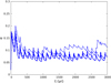 |
Fig. 17. Disk eccentricity, edisk, evolution under the perturbation of a binary system of e = 0.4. Values referring to different simulations are plotted: N = 20 000 (dotted line), N = 50 000 (dashed line), and N = 100 000 (full line). |
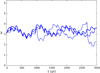 |
Fig. 18. Time evolution of argument of periastron, ωdisk, in an eccentric (e = 0.4) binary system. Like in Fig. 17, results for different simulations are illustrated: N = 20 000 (dotted line), N = 50 000 (dashed line), and N = 100 000 (full line). |
Similarly, Fig. 18 shows the mean inclination of the oscialltions in the disk semimajor axis around the initial value (which conventionally was taken as π). Even for the argument of periastron of the disk, a convergence can be observed near the simulations with higher resolution.
5. Summary and conclusions
The primary intent of this paper is the presentation, testing, and preliminary application of our new SPH code, GaSPH, which is designed to be a multi-purpose code that is applicable to a variety of astrophysical, multi-phase, and self-gravitating environments. We briefly summarize the main points below.
-
We presented and discussed the characteristics of our code in some detail. At the moment, the code does not treat radiative transfer, but properly takes internal gas gravity and the gas-star mutual gravity into account.
-
The code fully passes the classic tests in slowly varying situations, which assess its stability, and also in violently varying cases that reproduce the Sedov–Taylor blast wave well.
-
The code performs well numerically (speed) and has a good stability and quality, as we discussed in Sect. 3.2.
-
The capability of the code to treat the evolution of a protoplanetary disk when it interacts with a single star and with a binary star was tested.
In a near future, we aim to reach a much better resolution, which is achievable with an MPI parallel version of our code. This will allow us to study disks on the smaller, planetary, scale. Further scientific applications of our code will include the evolution of protoplanetary disks in a star cluster environment in order to study the star-to-disk feedback.
Acknowledgments
We express our gratitude to Fabrizio Capaccioni of INAF-IAPS-Istituto di Astrofisica e Planetologia Spaziali (Rome, Italy) for the valuable support and useful discussions throughout the preparation of this work. We also wish to thank the anonymous referee for the suggestions and comments that greatly helped to improve the paper.
References
- Aarseth, S. J. 1999, PASP, 111, 1333 [NASA ADS] [CrossRef] [Google Scholar]
- Allen, M. P., & Tildesley, D. J. 1989, Computer Simulation of Liquids (New York, USA: Clarendon Press) [Google Scholar]
- Andersen, H. C. 1983, J. Comput. Phys., 52, 24 [NASA ADS] [CrossRef] [Google Scholar]
- Armitage, P. J. 2011, ARA&A, 49, 195 [NASA ADS] [CrossRef] [EDP Sciences] [Google Scholar]
- Artymowicz, P., & Lubow, S. H. 1994, ApJ, 421, 651 [NASA ADS] [CrossRef] [Google Scholar]
- Attwood, R. E., Goodwin, S. P., & Whitworth, A. P. 2007, A&A, 464, 447 [NASA ADS] [CrossRef] [EDP Sciences] [Google Scholar]
- Balsara, D. S. 1995, J. Comput. Phys., 121, 357 [NASA ADS] [CrossRef] [Google Scholar]
- Barnes, J. E. 1986, The Use of Supercomputers in Stellar Dynamics: Proceedings of a Workshop Held at the Institute for Advanced Study Princeton, USA, June 2–4, 1986 (Berlin, Heidelberg: Springer, Berlin Heidelberg), 175 [CrossRef] [Google Scholar]
- Barnes, J., & Hut, P. 1986, Nature, 324, 446 [NASA ADS] [CrossRef] [Google Scholar]
- Baruteau, C., & Masset, F. 2008, ApJ, 678, 483 [NASA ADS] [CrossRef] [Google Scholar]
- Binney, J., & Tremaine, S. 1987, Galactic dynamics (Princeton, NJ: Princeton University Press) [Google Scholar]
- Boss, A. P. 1998, ApJ, 503, 923 [NASA ADS] [CrossRef] [Google Scholar]
- Boss, A. P. 2003, ApJ, 599, 577 [NASA ADS] [CrossRef] [Google Scholar]
- Capuzzo-Dolcetta, R., & Miocchi, P. 1998, J. Comput. Phys., 143, 29 [NASA ADS] [CrossRef] [Google Scholar]
- Capuzzo-Dolcetta, R., Spera, M., & Punzo, D. 2013, J. Comput. Phys., 236, 580 [NASA ADS] [CrossRef] [Google Scholar]
- Chandrasekhar, S. 1958, An Introduction to the Study of Stellar Structure (New York, US: Dover Publications, Inc.) [Google Scholar]
- Chapman, B., Jost, G., & Van Der Pas, R. 2007, Using OpenMP - Portable Shared Memory Parallel Programming (Cambridge, USA: The MIT Press) [Google Scholar]
- Ciardi, D. R., Crossfield, I. J. M., Feinstein, A. D., et al. 2018, AJ, 155, 10 [NASA ADS] [CrossRef] [Google Scholar]
- D’Alessio, P., Calvet, N., Hartmann, L., Lizano, S., & Cantó, J. 1999, ApJ, 527, 893 [NASA ADS] [CrossRef] [Google Scholar]
- Dullemond, C. P., Hollenbach, D., Kamp, I., & D’Alessio, P. 2007, Protostars and Planets V, 555 [Google Scholar]
- Feagin, T. 2012, Sci. Comput., 20, 437 [Google Scholar]
- Garcia, P. J. V. 2011, Physical Processes in Circumstellar Disks Around Young Stars (Chicago: The University of Chicago Press) [Google Scholar]
- Gingold, R. A., & Monaghan, J. J. 1977, MNRAS, 181, 375 [Google Scholar]
- Handy, J. 1998, The Cache Memory Book (USA: Academic Press, inc.) [Google Scholar]
- Hartmann, L., Calvet, N., Gullbring, E., & D’Alessio, P. 1998, ApJ, 495, 385 [NASA ADS] [CrossRef] [Google Scholar]
- Hernquist, L. 1987, ApJS, 64, 715 [NASA ADS] [CrossRef] [Google Scholar]
- Hernquist, L., & Katz, N. 1989, ApJS, 70, 419 [NASA ADS] [CrossRef] [Google Scholar]
- Hockney, R. W., & Eastwood, J. W. 1981, Computer Simulation Using Particles (New York: McGraw-Hill) [Google Scholar]
- Hockney, R. W., & Eastwood, J. W. 1988, Computer Simulation Using Particles (Bristol: Hilger) [CrossRef] [Google Scholar]
- Hosono, N., Saitoh, T. R., & Makino, J. 2016, ApJS, 224, 32 [NASA ADS] [CrossRef] [Google Scholar]
- Hubber, D. A., Allison, R. J., Smith, R., & Goodwin, S. P. 2013, MNRAS, 430, 1599 [NASA ADS] [CrossRef] [Google Scholar]
- Hut, P., Makino, J., & McMillan, S. 1995, ApJ, 443, L93 [NASA ADS] [CrossRef] [Google Scholar]
- Kratter, K., & Lodato, G. 2016, ARA&A, 54, 271 [NASA ADS] [CrossRef] [Google Scholar]
- Kratter, K. M., Matzner, C. D., & Krumholz, M. R. 2008, ApJ, 681, 375 [NASA ADS] [CrossRef] [Google Scholar]
- Liu, C.-J., Yao, Z., & Ding, W.-B. 2017, Res. Astron. Astrophys., 17, 078 [NASA ADS] [CrossRef] [Google Scholar]
- Lucy, L. B. 1977, AJ, 82, 1013 [NASA ADS] [CrossRef] [Google Scholar]
- Lynden-Bell, D., & Pringle, J. E. 1974, MNRAS, 168, 603 [NASA ADS] [CrossRef] [Google Scholar]
- Marzari, F., Scholl, H., Thébault, P., & Baruteau, C. 2009, A&A, 508, 1493 [NASA ADS] [CrossRef] [EDP Sciences] [Google Scholar]
- Masset, F. 2000, A&AS, 141, 165 [NASA ADS] [CrossRef] [EDP Sciences] [Google Scholar]
- Mayer, L., Quinn, T., Wadsley, J., & Stadel, J. 2002, Science, 298, 1756 [NASA ADS] [CrossRef] [PubMed] [Google Scholar]
- Meglicki, Z., Wickramasinghe, D., & Bicknell, G. V. 1993, MNRAS, 264, 691 [NASA ADS] [CrossRef] [Google Scholar]
- Meru, F., & Bate, M. R. 2012, MNRAS, 427, 2022 [NASA ADS] [CrossRef] [Google Scholar]
- Miocchi, P., & Capuzzo-Dolcetta, R. 2002, A&A, 382, 758 [NASA ADS] [CrossRef] [EDP Sciences] [Google Scholar]
- Monaghan, J. J. 1988, Comput. Phys. Commun., 48, 89 [Google Scholar]
- Monaghan, J. J. 1989, J. Comput. Phys., 82, 1 [NASA ADS] [CrossRef] [Google Scholar]
- Monaghan, J. J. 1992, ARA&A, 30, 543 [NASA ADS] [CrossRef] [Google Scholar]
- Monaghan, J. J. 2005, Rep. Progr. Phys., 68, 1703 [NASA ADS] [CrossRef] [Google Scholar]
- Monaghan, J. J., & Lattanzio, J. C. 1985, A&A, 149, 135 [NASA ADS] [Google Scholar]
- Morris, J. P., & Monaghan, J. J. 1997, J. Comput. Phys., 136, 41 [NASA ADS] [CrossRef] [MathSciNet] [Google Scholar]
- Nelson, A. F., Benz, W., Adams, F. C., & Arnett, D. 1998, ApJ, 502, 342 [NASA ADS] [CrossRef] [Google Scholar]
- Picogna, G., & Marzari, F. 2013, A&A, 556, A148 [NASA ADS] [CrossRef] [EDP Sciences] [Google Scholar]
- Pierens, A., & Nelson, R. P. 2007, A&A, 472, 993 [NASA ADS] [CrossRef] [EDP Sciences] [Google Scholar]
- Plummer, H. C. 1911, MNRAS, 71, 460 [CrossRef] [Google Scholar]
- Price, D. J., & Monaghan, J. J. 2007, MNRAS, 374, 1347 [NASA ADS] [CrossRef] [Google Scholar]
- Pringle, J. E. 1981, ARA&A, 19, 137 [NASA ADS] [CrossRef] [Google Scholar]
- Quinn, T., Katz, N., Stadel, J., & Lake, G. 1997, ArXiv e-prints [arXiv:astro-ph/9710043] [Google Scholar]
- Rosswog, S., & Price, D. 2007, MNRAS, 379, 915 [NASA ADS] [CrossRef] [Google Scholar]
- Rosswog, S., Davies, M. B., Thielemann, F.-K., & Piran, T. 2000, A&A, 360, 171 [NASA ADS] [Google Scholar]
- Saitoh, T. R., & Makino, J. 2009, ApJ, 697, L99 [NASA ADS] [CrossRef] [Google Scholar]
- Sedov, L. 1959, Similarity and Dimensional Methods in Mechanics (New York: CRC Press Inc.) [Google Scholar]
- Shakura, N. I., & Sunyaev, R. A. 1973, A&A, 24, 337 [NASA ADS] [Google Scholar]
- Springel, V. 2005, MNRAS, 364, 1105 [NASA ADS] [CrossRef] [Google Scholar]
- Springel, V., & Hernquist, L. 2002, MNRAS, 333, 649 [NASA ADS] [CrossRef] [Google Scholar]
- Stamatellos, D., Maury, A., Whitworth, A., & André, P. 2011, MNRAS, 413, 1787 [NASA ADS] [CrossRef] [Google Scholar]
- Tasker, E. J., Brunino, R., Mitchell, N. L., et al. 2008, MNRAS, 390, 1267 [NASA ADS] [CrossRef] [Google Scholar]
- Toomre, A. 1964, ApJ, 139, 1217 [Google Scholar]
Appendix A: Details of the numerical method
A.1. Velocity-Verlet method
At each time iteration, a and  are evaluated twice, in correspondence to the current step n and the next n + 1. Starting from a generic nth time iteration, we use a[n] and
 ![Mathematical equation: $ \dot{u}^{[n]} $](/articles/aa/full_html/2019/08/aa33143-18/aa33143-18-eq99.gif) to predict the velocity and the energy:
to predict the velocity and the energy:
![Mathematical equation: $$ \begin{aligned} {\left\{ \begin{array}{ll} \boldsymbol{v}^{*{[n+1]}} = \boldsymbol{v}^{[n]} + \boldsymbol{a}^{[n]} \Delta t \\ u ^{*[n+1]} = u^{[n]} + \dot{u}^{[n]} \Delta t \end{array}\right.}, \end{aligned} $$](/articles/aa/full_html/2019/08/aa33143-18/aa33143-18-eq100.gif) (A.1)
(A.1)
while the position is directly updated to the next step n + 1, without any prediction:
![Mathematical equation: $$ \begin{aligned} \boldsymbol{r}^{[n+1]} = \boldsymbol{r}^{[n]} + \boldsymbol{v}^{[n]} \Delta t + \dfrac{1}{2} \boldsymbol{a}^{[n]} \Delta t^2 . \end{aligned} $$](/articles/aa/full_html/2019/08/aa33143-18/aa33143-18-eq101.gif) (A.2)
(A.2)
With these new quantities, a new calculation is performed for a and  ; we thus have
![Mathematical equation: $$ \begin{aligned} {\left\{ \begin{array}{ll} \boldsymbol{a}^{*{[n+1]}} = \boldsymbol{a} \left( \boldsymbol{r}^{[n+1]},\boldsymbol{v}^{*{[n+1]}},u^{*[n+1]} \right) \\ \dot{u}^{*[n+1]} = \dot{u} \left( \boldsymbol{r}^{[n+1]},\boldsymbol{v}^{*[n+1]},u^{*[n+1]} \right) \end{array}\right.}, \end{aligned} $$](/articles/aa/full_html/2019/08/aa33143-18/aa33143-18-eq103.gif) (A.3)
(A.3)
which we can use to correct velocity and energy,
![Mathematical equation: $$ \begin{aligned} {\left\{ \begin{array}{ll} \boldsymbol{v}^{[n+1]} = \boldsymbol{v}^{[n]} + \left( \boldsymbol{a}^{[n]} + \boldsymbol{a}^{*[n+1]} \right) \dfrac{\Delta t}{2} \\ u^{[n+1]} = u^{[n]} + \left( \dot{u}^{[n]} + \dot{u}^{*[n+1]} \right) \dfrac{\Delta t}{2} \end{array}\right.}. \end{aligned} $$](/articles/aa/full_html/2019/08/aa33143-18/aa33143-18-eq104.gif) (A.4)
(A.4)
It can be straightforwardly shown that when acceleration only depends on the positions, that is, in a Newtonian problem without hydrodynamics, the Verlet method described above is equivalent to a standard second-order kick-drift-kick (KDK) leap-frog method. When the acceleration depends neither on the velocity field nor on the internal energy, the quantity a*[n + 1] corresponds to the actual acceleration a[n + 1] that is related to the next step. The numerical method can thus be rewritten in the following way:
![Mathematical equation: $$ \begin{aligned} {\left\{ \begin{array}{ll} \boldsymbol{r}^{[n+1]} = \boldsymbol{r}^{[n]} + \left( \boldsymbol{v}^{[n]} + \dfrac{1}{2} \boldsymbol{a}^{[n]} \Delta t \right) \Delta t = \boldsymbol{r}^{[n]} + \boldsymbol{v}^{[n+ 1/2]} \Delta t \\ \boldsymbol{v}^{[n+1]} = \boldsymbol{v}^{[n]} + \dfrac{1}{2} \boldsymbol{a}^{[n]} \Delta t + \dfrac{1}{2} \boldsymbol{a}^{[n]} \Delta t = \boldsymbol{v}^{[n+1/2]} + \boldsymbol{a}^{[n]} \dfrac{\Delta t}{2} \end{array}\right.}, \end{aligned} $$](/articles/aa/full_html/2019/08/aa33143-18/aa33143-18-eq105.gif) (A.5)
(A.5)
which represents indeed the standard expression of a KDK leap-frog integrator that requires just one force calculation per time step (see Hockney & Eastwood 1988; Hut et al. 1995; Quinn et al. 1997, for leap-frog methods and further improvements).
Each particles has its own individual time steps, sorted by the code as submultiples of the maximum time step Δtmax. For a generic particle of index i, the time step is calculated according to the criteria expressed by Eqs. (17) and (18) and approximated to the nearest value Δti = 2−P ⋅ Δtmax, where P is a positive integer number. The simple scheme in Fig. A.1 shows that a single time iteration between two consecutive steps n and n + 1 is performed between the time t[n] and t[n + 1] = t[n] + Δtmin, while a generic particle of index i is updated between two characteristic times: ![Mathematical equation: $ t_i^{[{\rm PREV}]} $](/articles/aa/full_html/2019/08/aa33143-18/aa33143-18-eq106.gif) and
and ![Mathematical equation: $ t_i^{\rm NEXT} = t_i^{[{\rm PREV}]} + \Delta t_i $](/articles/aa/full_html/2019/08/aa33143-18/aa33143-18-eq107.gif) . The routines dedicated to the neighbor search, to the hydrodynamic forces, and to the gas self-gravity are activated for the particle i only when its time step is synchronized, that is, if the conditions
. The routines dedicated to the neighbor search, to the hydrodynamic forces, and to the gas self-gravity are activated for the particle i only when its time step is synchronized, that is, if the conditions ![Mathematical equation: $ t^{[n]} = t_i^{[{\rm PREV}]} $](/articles/aa/full_html/2019/08/aa33143-18/aa33143-18-eq108.gif) or
or ![Mathematical equation: $ t^{[n+1]} = t_i^{[{\rm NEXT}]} $](/articles/aa/full_html/2019/08/aa33143-18/aa33143-18-eq109.gif) are satisfied. Figure A.2 shows a scheme of a single time iteration. First, the code sorts and maps all the particles by building the tree, calculating the quadrupole momentum and all the other key quantities related to the cubes. This operation is thus independent on the particle time steps. Then, the code runs the main cycles of neighbor search and acceleration computation. For each ith particle, it verifies whether the particle is synchronized at t = t[n], that is, whether the condition
are satisfied. Figure A.2 shows a scheme of a single time iteration. First, the code sorts and maps all the particles by building the tree, calculating the quadrupole momentum and all the other key quantities related to the cubes. This operation is thus independent on the particle time steps. Then, the code runs the main cycles of neighbor search and acceleration computation. For each ith particle, it verifies whether the particle is synchronized at t = t[n], that is, whether the condition ![Mathematical equation: $ t^{[n]} = t_i^{[{\rm PREV}]} $](/articles/aa/full_html/2019/08/aa33143-18/aa33143-18-eq110.gif) is satisfied. In that case, the algorithm computes the density
is satisfied. In that case, the algorithm computes the density ![Mathematical equation: $ \rho_i^{[{\rm PREV}]} $](/articles/aa/full_html/2019/08/aa33143-18/aa33143-18-eq111.gif) , the pressure
, the pressure ![Mathematical equation: $ P_i^{[{\rm PREV}]} $](/articles/aa/full_html/2019/08/aa33143-18/aa33143-18-eq112.gif) , the velocity gradient
, the velocity gradient ![Mathematical equation: $ {\boldsymbol{\nabla} \cdot \boldsymbol{v}}_i^{[{\rm PREV}]} $](/articles/aa/full_html/2019/08/aa33143-18/aa33143-18-eq113.gif) and the velocity rotor
and the velocity rotor ![Mathematical equation: $ {\boldsymbol{\nabla} \times \boldsymbol{v}}_i^{[{\rm PREV}]} $](/articles/aa/full_html/2019/08/aa33143-18/aa33143-18-eq114.gif) , the switching coefficient of Eq. (12), the quantities
, the switching coefficient of Eq. (12), the quantities ![Mathematical equation: $ \omega_i^{[{\rm PREV}]}, \zeta_i^{[{\rm PREV}]} $](/articles/aa/full_html/2019/08/aa33143-18/aa33143-18-eq115.gif) , the hydrogravitational acceleration
, the hydrogravitational acceleration ![Mathematical equation: $ \boldsymbol{a}_i^{[{\rm PREV}]} $](/articles/aa/full_html/2019/08/aa33143-18/aa33143-18-eq116.gif) , and the time variation of the internal energy
, and the time variation of the internal energy ![Mathematical equation: $ \dot{u}_i^{[\mathrm{PREV}]} $](/articles/aa/full_html/2019/08/aa33143-18/aa33143-18-eq117.gif) . These quantities are suitably stored in memory, to be used in further phases of the integration and in further iterations. For the remaining nonsynchronized particles, the algorithm indeed uses the quantities that were calculated in previous stages.
. These quantities are suitably stored in memory, to be used in further phases of the integration and in further iterations. For the remaining nonsynchronized particles, the algorithm indeed uses the quantities that were calculated in previous stages.
 |
Fig. A.1. Sketch of the hierarchical time-step subdivision. A generic individual time step, Δti is a power of two multiples of the minimum time step Δtmin, and a power of two submultiple of the maximum one, Δtmax. The integration is performed by means of elementary iterations from t[n] to t[n + 1] = t[n] + Δtmin, while the particle is updated from t[PREV] to t[NEXT] = t[PREV] + Δti. The hydrodynamics and force routines are activated only for particles that are synchronized at t[n] = t[PREV] or at t[n + 1] = t[NEXT]. |
 |
Fig. A.2. Flow chart showing the main scheme of a single time iteration. |
If some stars are included in the simulation, ![Mathematical equation: $ a_i^{[{\rm PREV}]} $](/articles/aa/full_html/2019/08/aa33143-18/aa33143-18-eq118.gif) is incremented by a contribution from the star-gas interaction for every ith particle.
is incremented by a contribution from the star-gas interaction for every ith particle.
After this, we update the time of v, u, and r. For particles synchronized at t = t[n + 1], so that ![Mathematical equation: $ t_i^{[{\rm NEXT}]}=t^{[n+1]} $](/articles/aa/full_html/2019/08/aa33143-18/aa33143-18-eq119.gif) , the velocity and the energy are updated with the same predictor scheme as expressed by Eq. (A.1), thus, we have
, the velocity and the energy are updated with the same predictor scheme as expressed by Eq. (A.1), thus, we have
![Mathematical equation: $$ \begin{aligned} {\left\{ \begin{array}{ll} \boldsymbol{v}_i^{*[n+1]} = \boldsymbol{v}_i^{*[\mathrm{NEXT}]} = \boldsymbol{v}_i^{[\mathrm{PREV}]} + \boldsymbol{a}_i^{[\mathrm{PREV}]} \Delta t_i \\ u_i^{*[n+1]} = u_i^{*[\mathrm{NEXT}]} = u_i^{[\mathrm{PREV}]} + \dot{u_i}^{[\mathrm{PREV}]} \Delta t_i \end{array}\right.}. \end{aligned} $$](/articles/aa/full_html/2019/08/aa33143-18/aa33143-18-eq120.gif) (A.6)
(A.6)
The position is updated as well, in the same manner as indicated by Eq. (A.2):
![Mathematical equation: $$ \begin{aligned} \boldsymbol{r_i}^{[n+1]} = \boldsymbol{r}_i^{[\mathrm{NEXT}]} = \boldsymbol{r}_i^{[\mathrm{PREV}]} + \boldsymbol{v}_i^{[\mathrm{PREV}]} \Delta t_i + \dfrac{1}{2} \boldsymbol{a}_i^{[\mathrm{PREV}]} \Delta t_i^2 . \end{aligned} $$](/articles/aa/full_html/2019/08/aa33143-18/aa33143-18-eq121.gif) (A.7)
(A.7)
On the other hand, for nonsynchronized points, we do not update, but estimate the quantities v*[n + 1], u*[n + 1] and r[n + 1] by means of the following predictor scheme:
![Mathematical equation: $$ \begin{aligned} {\left\{ \begin{array}{ll} \boldsymbol{v}_i^{*[n+1]} = \boldsymbol{v}_i^{[\mathrm{PREV}]} + \boldsymbol{a}_i^{[\mathrm{PREDICT}]} \delta t_i \\ u_i^{*[n+1]} = u_i^{[\mathrm{PREV}]} + \dot{u}_i^{[\mathrm{PREV}]} \delta t_i \\ \boldsymbol{r}_i^{[n+1]} = \boldsymbol{r_i}^{[\mathrm{PREV}]} + \boldsymbol{v}_i^{[\mathrm{PREDICT}]} \delta t_i + \dfrac{1}{2}\boldsymbol{a}_i^{[\mathrm{PREDICT}]} \delta t_i^2, \end{array}\right.} \end{aligned} $$](/articles/aa/full_html/2019/08/aa33143-18/aa33143-18-eq122.gif) (A.8)
(A.8)
which contains the following quantities:
![Mathematical equation: $$ \begin{aligned}&\delta t_i = t^{[n+1]} - t_i^{[\mathrm{PREV}]} \\&\boldsymbol{a}_i^{[\mathrm{PREDICT}]} = \frac{1}{2}\left(\boldsymbol{a}_i^{[\mathrm{PREV}]} + \boldsymbol{a}_i^{[n]}\right) \\&\boldsymbol{v}_i^{[\mathrm{PREDICT}]} = \frac{1}{2}\left(\boldsymbol{v}_i^{[\mathrm{PREV}]} + \boldsymbol{v}_i^{*[n+1]}\right) \end{aligned} $$](/articles/aa/full_html/2019/08/aa33143-18/aa33143-18-eq123.gif)
![Mathematical equation: $ \boldsymbol{a}_i^{[n]} $](/articles/aa/full_html/2019/08/aa33143-18/aa33143-18-eq124.gif) is exactly equal to the old value
is exactly equal to the old value ![Mathematical equation: $ \boldsymbol{a}_i^{[{\rm PREV}]} $](/articles/aa/full_html/2019/08/aa33143-18/aa33143-18-eq125.gif) in simulations with pure gas because the algorithm does not compute the acceleration at the current iteration. When one or more stars interact with the gas, however, the two accelerations are different because they contain different contributions from the gas-star interaction, which is independently calculated at every step in the particle synchronization.
in simulations with pure gas because the algorithm does not compute the acceleration at the current iteration. When one or more stars interact with the gas, however, the two accelerations are different because they contain different contributions from the gas-star interaction, which is independently calculated at every step in the particle synchronization.
Based on the new velocities, energies, and space coordinates, a second phase of recalculating the hydrodynamical variables and the accelerations occurs, of course, which is limited to the synchronized points at t = t[n + 1]. Thus, each synchronized ith particle owns the following updated hydrodynamical quantities: ![Mathematical equation: $ \rho_i^{[{\rm NEXT}]} $](/articles/aa/full_html/2019/08/aa33143-18/aa33143-18-eq126.gif) ,
, ![Mathematical equation: $ P_i^{[{\rm NEXT}]} $](/articles/aa/full_html/2019/08/aa33143-18/aa33143-18-eq127.gif) ,
, ![Mathematical equation: $ {\boldsymbol{\nabla} \cdot \boldsymbol{v}}_i^{[{\rm NEXT}]} $](/articles/aa/full_html/2019/08/aa33143-18/aa33143-18-eq128.gif) ,
, ![Mathematical equation: $ {\boldsymbol{\nabla} \times \boldsymbol{v}}_i^{[{\rm NEXT}]} $](/articles/aa/full_html/2019/08/aa33143-18/aa33143-18-eq129.gif) ,
, ![Mathematical equation: $ f_i^{[{\rm NEXT}]} $](/articles/aa/full_html/2019/08/aa33143-18/aa33143-18-eq130.gif) ,
, ![Mathematical equation: $ \omega_i^{[{\rm NEXT}]} $](/articles/aa/full_html/2019/08/aa33143-18/aa33143-18-eq131.gif) and
and ![Mathematical equation: $ \zeta_i^{[{\rm NEXT}]} $](/articles/aa/full_html/2019/08/aa33143-18/aa33143-18-eq132.gif) . The accelerations and energy can thus be computed in the same manner as shown by Eq. (A.3):
. The accelerations and energy can thus be computed in the same manner as shown by Eq. (A.3):
![Mathematical equation: $$ \begin{aligned} {\left\{ \begin{array}{ll} \boldsymbol{a}_i^{*[n+1]} = \boldsymbol{a}_i^{*[\mathrm{NEXT}]} = \boldsymbol{a} \left( \boldsymbol{r}_i^{[\mathrm{NEXT}]},\boldsymbol{v}_i^{*[\mathrm{NEXT}]},u_i^{*[\mathrm{NEXT}]} \right) \\ \dot{u}^{*[n+1]} = \dot{u}^{*[\mathrm{NEXT}]} = \dot{u} \left( \boldsymbol{r}_i^{[\mathrm{NEXT}]},\boldsymbol{v}_i^{*[\mathrm{NEXT}]},u_i^{*[\mathrm{NEXT}]} \right) \end{array}\right.}. \end{aligned} $$](/articles/aa/full_html/2019/08/aa33143-18/aa33143-18-eq133.gif) (A.9)
(A.9)
Then, by applying the same formalism as expressed by Eq. (A.4), energy and velocities can be finally updated:
![Mathematical equation: $$ \begin{aligned} {\left\{ \begin{array}{ll} \boldsymbol{v}_i^{[n+1]} = \boldsymbol{v}_i^{[\mathrm{NEXT}]} = \boldsymbol{v}^{[\mathrm{PREV}]} + \left( \boldsymbol{a}_i^{[\mathrm{PREV}]} + \boldsymbol{a}_i^{*[\mathrm{NEXT}]} \right) \dfrac{\Delta t_i}{2} \\ u_i^{[n+1]} = u_i^{[\mathrm{NEXT}]} = u_i^{[\mathrm{PREV}]} + \left( \dot{u}_i^{[\mathrm{PREV}]} + \dot{u}_i^{*[\mathrm{NEXT}]} \right) \dfrac{\Delta t_i}{2} \end{array}\right.}. \end{aligned} $$](/articles/aa/full_html/2019/08/aa33143-18/aa33143-18-eq134.gif) (A.10)
(A.10)
A.2. 14th-order Runge–Kutta method
For a generic set of Nob objects we wish to integrate the following differential equations that are associated with a generic ith object:
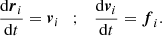 (A.11)
The method begins with a first estimation of the explicit derivatives at the iteration n:
![Mathematical equation: $$ \begin{aligned} {\left\{ \begin{array}{ll} \boldsymbol{Kv}_{1}^{(i)} = \boldsymbol{f} ( \boldsymbol{r}_1^{[n]},\boldsymbol{r}_2^{[n]}, \ldots , \boldsymbol{r}_i^{[n]}, \ldots , \boldsymbol{r}_N^{[n]} ) \\ \boldsymbol{Kr}_{1}^{(i)} = \boldsymbol{v}_i^{[n]} \end{array}\right.}, \end{aligned} $$](/articles/aa/full_html/2019/08/aa33143-18/aa33143-18-eq136.gif) (A.12)
(A.12)
which can be used to estimate the further quantities corresponding to a second substep n + c2:
![Mathematical equation: $$ \begin{aligned}&\boldsymbol{Kv}_{2}^{(i)} = \boldsymbol{f} ( \boldsymbol{r}_1^{[n+c2]}, \boldsymbol{r}_2^{[n+c2]}, \ldots , \boldsymbol{r}_i^{[n+c2]}, \ldots , \boldsymbol{r}_N^{[n+c2]} ) \nonumber \\&\boldsymbol{Kr}_{2}^{(i)} = \boldsymbol{v}_i^{[n]} + a_{21} \boldsymbol{Kv}_{1}^{(i)} \Delta t , \end{aligned} $$](/articles/aa/full_html/2019/08/aa33143-18/aa33143-18-eq137.gif) (A.13)
(A.13)
where ![Mathematical equation: $ \boldsymbol{r}_i^{[n+c2]} = \boldsymbol{r}_i^{[n]} + a_{21} \boldsymbol{Kr}_{1}^{(i)} \Delta t ~~ $](/articles/aa/full_html/2019/08/aa33143-18/aa33143-18-eq138.gif) represents the ith particle position updated to an intermediate time t + c2Δt. In the same manner, further consecutive estimations of βth terms can be performed:
represents the ith particle position updated to an intermediate time t + c2Δt. In the same manner, further consecutive estimations of βth terms can be performed:
![Mathematical equation: $$ \begin{aligned}&\boldsymbol{Kv}_{\beta }^{(i)} = \boldsymbol{f} ( \boldsymbol{r}_1^{[n+c\beta ]}, \boldsymbol{r}_2^{[n+c\beta ]}, \ldots , \boldsymbol{r}_i^{[n+c\beta ]}, \ldots , \boldsymbol{r}_N^{[n+c\beta ]} ) \nonumber \\&\boldsymbol{Kr}_{\beta }^{(i)} = \boldsymbol{r}_i^{[n]} + \sum \limits _{\gamma =1}^{\beta -1} a_{\beta \gamma } \boldsymbol{Kv}_{\gamma }^{(i)}~\Delta t, \end{aligned} $$](/articles/aa/full_html/2019/08/aa33143-18/aa33143-18-eq139.gif) (A.14)
(A.14)
with ![Mathematical equation: $ \boldsymbol{r}_i^{[n+c\beta]} = \boldsymbol{r}_i^{[n]} + \sum\limits _{\gamma=1}^{\beta -1} a_{\beta\gamma} \boldsymbol{Kr}_{\gamma }^{(i)} \Delta t $](/articles/aa/full_html/2019/08/aa33143-18/aa33143-18-eq140.gif) the vector position of the ith particle at a generic intermediate time t + cβΔt. Because γ < β, every quantity explicitly depends on previous estimations. The coefficients aβγ are the elements of a 35 × 34 matrix, while bβ and cβ represent two arrays of 35 elements. The matrix a requires the following restriction:
the vector position of the ith particle at a generic intermediate time t + cβΔt. Because γ < β, every quantity explicitly depends on previous estimations. The coefficients aβγ are the elements of a 35 × 34 matrix, while bβ and cβ represent two arrays of 35 elements. The matrix a requires the following restriction:
 (A.15)
Since we work with a fully explicit method, a is triangular, and aβγ = 0, for γ > β. In total, each star will have 35 velocity RK coefficients Krβ and 35 acceleration RK coefficients Kvβ, the resulting velocity and position at the next time step will be given by
![Mathematical equation: $$ \begin{aligned}&\boldsymbol{v}_i^{[n+1]} = \boldsymbol{v}_i^{[n]} + \sum \limits _{\beta =1}^{35} b_{\beta } \boldsymbol{Kv}_{\beta }^{(i)} \Delta t \nonumber \\&\boldsymbol{r}_i^{[n+1]} = \boldsymbol{r}_i^{[n]} + \sum \limits _{\beta =1}^{35} b_{\beta } \boldsymbol{Kr}_{\beta } ^{(i)} \Delta t. \end{aligned} $$](/articles/aa/full_html/2019/08/aa33143-18/aa33143-18-eq142.gif) (A.16)
(A.16)
To integrate the time evolution of a system composed of both gas and stars, we coupled the Verlet and the RK integration methods as follows. At the starting iteration n, the gas particles feel the gravity field from the stars, the mutual interactions of the SPH, and eventually, its self-gravity. Then, v*[n + 1] and u*[n + 1] are predicted, and their positions are thus updated according to Eq. (A.2). At the same time, the star positions and velocities were first updated with the Runge–Kutta method, then, the explicit force contributions due to the SPH particles ![Mathematical equation: $ \boldsymbol{a}_{\mathrm{part}}^{[n]} $](/articles/aa/full_html/2019/08/aa33143-18/aa33143-18-eq143.gif) were added to Eq. (A.16). Stars and SPH particles were coupled by direct point-to-point interaction, without any approximation for the gravitational field. Finally, we corrected the gas positions and velocity according to Eq. (A.4) by recalculating the accelerations and the energy rates at the new stage n + 1.
were added to Eq. (A.16). Stars and SPH particles were coupled by direct point-to-point interaction, without any approximation for the gravitational field. Finally, we corrected the gas positions and velocity according to Eq. (A.4) by recalculating the accelerations and the energy rates at the new stage n + 1.
Appendix B: Technical features
B.1. Neighbor search and acceleration updating
Before we employed it to compute gravitational interactions, the tree grid was also used to support the operations related to the nearest-neighbor search. To calculate the density and the smoothing length, each ith particle starts with a first-guess value of hi and makes a tree walk by adopting an opening criterion that is slightly different from Eqs. (20) and (21). Given a generic particle of index i, in order to find the other points enclosed in its SPH kernel support, we checked for each cube the overlap with a sphere of radius 2hi centered onto the point ri = (xi, yi, zi). A box is opened only if the following three conditions are valid:
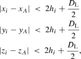 (B.1)
(B.1)
where (xA, yA, zA) are the coordinates of the geometrical center of the cube and DL is its side length. The tree walk continues by opening the further cubes according to the last rule, until the single particles are reached and the neighborhood is thus determined. At the end of the walk, a temporary value of density ρi is calculated. If the number of encountered neighbors differs from the expected number (and the difference exceeds the tolerance number), hi is updated according to Eq. (5). Then, a new tree walk is performed, and a new value for the density is computed. The tree walk and the hi, ρi updating are executed cyclically until the number of neighbors converges on the desired value. During the tree walk, the various quantities Pi, Ωi, ζi, f, ∇ ⋅ vi, and ∇ × vi are computed at the same time together with the density.
After this preliminary phase, the acceleration a and the thermal energy rate  can be computed by performing a further tree walk for each particle. During the walk, the hydrodynamics contribution to the acceleration and the gravity field are computed at the same time. For each box, before Eq. (20) (or Eq. (21)) is applied, the code primarily checks Eq. (B.1) to distinguish cubes that might contain some neighbor particles for the SPH interpolation. If this is satisfied, the box is opened, otherwise the particles inside will not contribute at all to hydrodynamics. After this primary check, the algorithm performs a secondary control by applying the opening criterion of Eq. (20) (or Eq. (21)) to decide whether the multipole approximation can be applied to the Newtonian field. As a result, practically, a generic ith particle will interact with its local SPH neighborhood following Eqs. (7) and (8), experiencing the Newtonian force through a direct particle-to-particle interaction. The remaining particles that lie outside the SPH domain contribute to the accelerations with or without multipole approximation, according to the basic criteria of Eq. (20) or (21).
During the computation of acceleration terms, ai, the neighbor domain search process may suffer some technical problems. The interpolation of the density (Eq. (6)) together with interpolations (9), (10), (12), and (13) are rather straightforward to perform because they require a sum over a domain that only depends on the local hi. On the other hand, Eq. (7) contains sums that extend over a more complex region because the W and gsoft functions depend not only on the local smoothing length, but also on the hj, which characterizes the domain extension of a surrounding jth particle. The condition of Eq. (B.1) guarantees that we can find all the nearest jth particles with a smoothing length hj ≤ hi. Nevertheless, particles with hj > hi also exist for which 2hj is smaller than the mutual distance rij. They give a non-null contribution to the acceleration of the ith point, but they are excluded from the neighbor search, and the code does not take them into account, which leads to an incorrect implementation of the SPH equations. It is rather easy to solve this problem when the algorithm works with a uniform time step. Equation (7) contains pairs of terms that are symmetric with respect to the swap of indexes i − j; moreover, one term of each pair depends only on hi, while the other depends only on hj. This means that when the ith particle walks along the tree and finds the jth particle within the interpolation domain 2hi, the code may add to ai the quantity 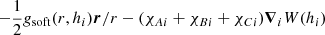 , and may add to aj the same quantity with the opposite sign. Here we used the following expressions for a generic particle of ith index:
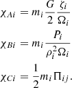 (B.2)
(B.2)
When the jth particle in turn makes the tree walk, the code can find the ith particle within the domain 2hj. In this case, the quantity  is added to aj and the same quantity with opposite sign is added to ai.
This technique cannot be applied when an individual time step is assigned to each particle because during the force computation some particles are inactive and the symmetry of Eq. (7) is thus broken. When the ith particle is active and the jth particle is inactive and lies outside the radius 2hi, the algorithm adds to ai the full set of terms in Eq. (7) to take into account the contributions of the jth point, and it increases the neighbor-search radius. This means that only during the second-step tree walk does the code apply the criterion in Eq. (B.1) with a slight modification of the radius because a value higher than 2hi is used, which is estimated as follows. The algorithm calculates a local interpolation of the gradient of the softening length, estimated as
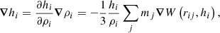 (B.3)
(B.3)
which is computed in the same loop as was used for the density. Then, in place of hi, the code uses the quantity ![Mathematical equation: $ h_i \cdot \max \left( \delta_h h_i^{[{\rm MAX}]}/h_i,\,1 + |\boldsymbol{\nabla}h_i|\right) $](/articles/aa/full_html/2019/08/aa33143-18/aa33143-18-eq150.gif) , with δh a suitable constant that we set to 1.3. The quantity
, with δh a suitable constant that we set to 1.3. The quantity ![Mathematical equation: $ h_i^{[{\rm MAX}]} $](/articles/aa/full_html/2019/08/aa33143-18/aa33143-18-eq151.gif) represents an estimate of the maximum local value of the softening length. It tries to probe all the neighbors jth particles, including the points outside the radius 2hi, that can make an SPH interaction with the ith particle, that is, such that hj > hi ∨ 2hj > rij. In an earlier time step, when the jth particle is active, we therefore determine whether the length hj is greater than the local maximum length around the ith position. This scheme increases the CPU time by increasing the direct point-to-point interactions. Nevertheless, it involves just local interactions, and as N increases, the CPU efforts become increasingly less relevant compared with the nonlocal gravity computations that are performed with the tree scheme. This method empirically represents a correct technique for finding the neighbors of a point in case of individual time steps, even though it cannot be mathematically proven that it is able to find 100% of the effective neighbor particles in all possible density configurations. We conducted a series of tests in which we even employed extreme density contrasts like in the case of a Sedov–Taylor blast-wave profile, and found that 100% of the effective neighbor particles were found when δh was above 1.2.
represents an estimate of the maximum local value of the softening length. It tries to probe all the neighbors jth particles, including the points outside the radius 2hi, that can make an SPH interaction with the ith particle, that is, such that hj > hi ∨ 2hj > rij. In an earlier time step, when the jth particle is active, we therefore determine whether the length hj is greater than the local maximum length around the ith position. This scheme increases the CPU time by increasing the direct point-to-point interactions. Nevertheless, it involves just local interactions, and as N increases, the CPU efforts become increasingly less relevant compared with the nonlocal gravity computations that are performed with the tree scheme. This method empirically represents a correct technique for finding the neighbors of a point in case of individual time steps, even though it cannot be mathematically proven that it is able to find 100% of the effective neighbor particles in all possible density configurations. We conducted a series of tests in which we even employed extreme density contrasts like in the case of a Sedov–Taylor blast-wave profile, and found that 100% of the effective neighbor particles were found when δh was above 1.2.
B.2. Optimization of the tee-code memory
The development of increasingly faster RAM memory architectures in the past years is promising. The CPU clock speed is no longer the only parameter that substantially affects the performance of a program. In order to write efficient algorithms, the number of CPU operations has to be minimized and the data need to be suitably stored in memory to be red as fast as possible. Moreover, modern architectures support a huge amount of cache memory, with orders of magnitude from 1 MB to 102 MB. The cache represents a refined and fast-readable level of memory close to the CPU (for an exhaustive essay on cache memory architectures, we refer to Handy 1998). Each time a system needs to manipulate some data, a little chunk of memory in which the relative variables are contained is gathered from the RAM and copied into the cache, from which the processor can operate very quickly. For these reasons, the efficiency of an algorithm is strictly connected to its ability to make several consecutive operations using variables that are stored very close in memory. In this way, the data are loaded once into the cache and the CPU compute directly by minimizing the memory traffic with the RAM. For these purposes, it is straightforward to write efficient tree codes, and more specifically for our purposes, SPH algorithms, if the information related to the particles and cubes is suitably ordered inside the RAM. Barnes (1986) remarked that the particles should be ordered in memory according to their Cartesian position coordinates. The sorting criterion should accurately follow the same arrangement in which the boxes are mapped inside the RAM. Following this prescription, the closer the particles, the closer the areas of memory in which they are stored, and the closer the information of the related cubes.
B.3. OMP parallelization
By exploiting the OpenMP® libraries designed for Fortran-90, the code can even run with shared memory multi-core CPUs (see Chapman et al. 2007, for a modern treatment of the OpenMP paradigm). We implemented a parallelization for the density evaluation routine and for the acceleration field routine, so that different threads perform calculations on different particles. Given a generic ith point, the algorithm may need to update the quantities ai and  by summing two or more different contributions at the same time. The so-called data-race problem arises: two or more threads are accessed and update the same memory location at the same time, which leads to errors in storing the correct values. To overcome these problems, each thread is provided with a private array to store partial values of acceleration and internal energy rate. After the tree descent, these temporary arrays are summed.
All Tables
Work profiling (in percentage with respect to the total) of GaSPH, tested on a Plummer gas distribution with 20 stars and different numbers of SPH (first column).
All Figures
|
Fig. 1. Schematic 2D example of the lack of accuracy in the field computation caused by a large offset ΔCM. The center of gravity is far away from the ith particle, and the cube is not opened. Nevertheless, some particles that lie near the edge of the box, such as the jth and the kth points, are very close to the ith point, but their direct contribution is missed, which results in a loss of accuracy. |
| In the text | |
|
Fig. 2. Oscillation of the virial ratio as a function of time for different choices of code configuration parameters for the simulation of a Plummer distribution of 105 equal-mass particles. The continuous line shows θ = 0.6, ϵ = 0.2; the dashed line represents θ = 1.0, ϵ = 0.2; the dotted line shows θ = 0.6, ϵ = 0.5; and the dash-dotted line denotes θ = 1.0, ϵ = 0.5. |
| In the text | |
|
Fig. 3. Radial density profiles of the Sedov–Taylor blast wave at several times (increasing rightward) t = 0.05 (circles), t = 0.1 (triangles), and t = 0.2 (squares) in a simulation with N = 106. The results obtained using a higher resolution (N = 3 375 000) are plotted with dotted lines. The full lines represent the classical Sedov–Taylor auto-similar solutions. |
| In the text | |
|
Fig. 4. Equilibrium analytical solutions of the density profiles ρ(r) related to three different models of polytropes with indexes n = 1, n = 3/2, and n = 2, drawn as solid curves. Comparison with the computed profiles (dots). |
| In the text | |
|
Fig. 5. Lagrangian radii as a function of time for a hydro-Plummer distribution at equilibrium (see Sect. 3.1.4). The radii are normalized to their respective initial values. |
| In the text | |
|
Fig. 6. Radial density profile for a Plummer distribution with 50 000 SPH particles (solid line). The results obtained with Gadget-2 are also shown (dashed line). The analytical Plummer profile is plotted with a dotted line. The density is in units such that ρ0 = 3/(4π). |
| In the text | |
|
Fig. 7. Logarithmic ratio ρN/ρA of the numerical to analytical radial density profile for a Plummer distribution with 50 000 SPH particles (solid line). The results obtained with Gadget-2 are also shown (dashed line). |
| In the text | |
|
Fig. 8. Fractional variation in the z-component of the angular momentum for our simulated rotating Plummer model (see Sect. 3.1.5). We plot the results obtained by varying some configuration parameters: αmin = 0.1, b−1 = 5 (full line), αmin = 0.02, b−1 = 5 (dotted line), and αmin = 0.1, b−1 = 7 (dash-dotted line). |
| In the text | |
|
Fig. 9. CPU time per particle for the pure gravitational force calculation in monopole and quardupole approximations at different N. Gadget-2 results (empty circles) are compared to our code results (squares connected with dashed lines) in the same monopole approximation. The continuous line refers to the performance of GaSPH, and the quadrupole term is included in the field. |
| In the text | |
|
Fig. 10. GaSPH average CPU times per particle as a function of N. Comparison of different routines: SPH neighbor-search routine averaged for a single iteration (circles), pure gravity computation with monopole term (empty squares) and with quadrupole term (filled squares), self-gravity computation up to quadrupole and including the SPH terms (triangles). The units are the same as in Fig. 9. |
| In the text | |
|
Fig. 11. Number of processed particles per second. The continuous lines and the dashed lines refer to results with and without the correction term ΔCM, respectively. We show the simple gravity field calculation (empty circles) and the full self-gravity routine with hydrodynamics (squares). The quadrupole term is considered for the gravity field. θ = 0.6. |
| In the text | |
|
Fig. 12. Computational time per particle vs. log N for various values of the opening angle θ. The pure tree gravitational algorithm (dashed line) and full SPH+gravity algorithm are shown as dashed and solid lines, respectively. The quadrupole term is included in the force evaluation. The ΔrCM offset term is not considered by the opening criterion. |
| In the text | |
|
Fig. 13. Tree code relative errors Err(ak) (averaged over all the three Cartesian coordinates) for the gravitational field computation as a function of the CPU time. The data are illustrated for different particle numbers (N = 104, N = 105, and N = 106) in panels a, b, and c. In each panel, the full line connects the points related to a computation of the gravitational field made with the quadrupole approximation, while the dashed line refers to computations made by using just the monopole term. The shape of the “void” markers distinguishes different choices of θ with the “standard” criterion (Eq. (20)): θ = 0.8 (void squares), θ = 0.6 (void triangles), and θ = 0.4 (void circles). Results for different opening angles with the “opening law” (Eq. (21)) criterion are also marked: θ = 0.8 (solid squares), θ = 0.6 (solid triangles), and θ = 0.4 (solid circles). |
| In the text | |
|
Fig. 14. Surface density profiles Σ(R) of the disk at different times (t = 0 corresponds to the disk state after it has been relaxed up to a time of 50 000 yr). The dots represent the numerical results, while the lines refer to the analytical model (Eq. (35)). The actual initial disk setting (black triangles) is reported for the sake of comparison with the relaxed state. The abscissa is in AU and the density is expressed in 10−2 M⊙ AU−2. The evolved density profiles at t > 0 (t = 330 000 yr and t = 1 000 000 yr) are shifted down by −3 and −6 in logarithm, respectively, for clarity. The fitting curve of the density profile at t = 0 is also plotted (full lines). |
| In the text | |
|
Fig. 15. Relative (percentage) mass-loss rate of the disk |
| In the text | |
|
Fig. 16. Logarithm of the numerical radial profile of the disk density at t′=850 000 yr (dots). The density profile at the beginning of the simulation is also plotted (black triangles). The density at t = t′ matches the self-similar solution (Eq. (36)) with a parameter |
| In the text | |
|
Fig. 17. Disk eccentricity, edisk, evolution under the perturbation of a binary system of e = 0.4. Values referring to different simulations are plotted: N = 20 000 (dotted line), N = 50 000 (dashed line), and N = 100 000 (full line). |
| In the text | |
|
Fig. 18. Time evolution of argument of periastron, ωdisk, in an eccentric (e = 0.4) binary system. Like in Fig. 17, results for different simulations are illustrated: N = 20 000 (dotted line), N = 50 000 (dashed line), and N = 100 000 (full line). |
| In the text | |
|
Fig. A.1. Sketch of the hierarchical time-step subdivision. A generic individual time step, Δti is a power of two multiples of the minimum time step Δtmin, and a power of two submultiple of the maximum one, Δtmax. The integration is performed by means of elementary iterations from t[n] to t[n + 1] = t[n] + Δtmin, while the particle is updated from t[PREV] to t[NEXT] = t[PREV] + Δti. The hydrodynamics and force routines are activated only for particles that are synchronized at t[n] = t[PREV] or at t[n + 1] = t[NEXT]. |
| In the text | |
|
Fig. A.2. Flow chart showing the main scheme of a single time iteration. |
| In the text | |
Current usage metrics show cumulative count of Article Views (full-text article views including HTML views, PDF and ePub downloads, according to the available data) and Abstracts Views on Vision4Press platform.
Data correspond to usage on the plateform after 2015. The current usage metrics is available 48-96 hours after online publication and is updated daily on week days.
Initial download of the metrics may take a while.