| Issue |
A&A
Volume 628, August 2019
|
|
|---|---|---|
| Article Number | A41 | |
| Number of page(s) | 28 | |
| Section | Stellar atmospheres | |
| DOI | https://doi.org/10.1051/0004-6361/201731674 | |
| Published online | 06 August 2019 | |
Activity and rotation of the X-ray emitting Kepler stars
1
INAF – Istituto di Astrofisica Spaziale e Fisica Cosmica Milano,
via E. Bassini 15,
20133
Milano,
Italy
e-mail: This email address is being protected from spambots. You need JavaScript enabled to view it.
2
Università degli Studi dell’ Insubria,
Via Ravasi 2,
21100
Varese,
Italy
3
Institut für Astronomie & Astrophysik, Eberhard-Karls-Universität Tübingen,
Sand 1,
72076
Tübingen, Germany
4
INAF – Osservatorio Astronomico di Palermo, Piazza del Parlamento 1,
90134
Palermo, Italy
5
INAF – Osservatorio Astronomico di Brera,
via E. Bianchi 46,
23807
Merate (LC),
Italy
6
INFN – Istituto Nazionale di Fisica Nucleare, Sezione di Pavia,
via A. Bassi 6,
27100
Pavia,
Italy
Received:
30
July
2017
Accepted:
12
June
2019
Abstract
The relation between magnetic activity and rotation in late-type stars provides fundamental information on stellar dynamos and angular momentum evolution. Rotation-activity studies found in the literature suffer from inhomogeneity in the measurement of activity indexes and rotation periods. We overcome this limitation with a study of the X-ray emitting, late-type main-sequence stars observed by XMM-Newton and Kepler. We measured rotation periods from photometric variability in Kepler light curves. As activity indicators, we adopted the X-ray luminosity, the number frequency of white-light flares, the amplitude of the rotational photometric modulation, and the standard deviation in the Kepler light curves. The search for X-ray flares in the light curves provided by the EXTraS (Exploring the X-ray Transient and variable Sky) FP-7 project allows us to identify simultaneous X-ray and white-light flares. A careful selection of the X-ray sources in the Kepler field yields 102 main-sequence stars with spectral types from A to M. We find rotation periods for 74 X-ray emitting main-sequence stars, 20 of which do not have period reported in the previous literature. In the X-ray activity-rotation relation, we see evidence for the traditional distinction of a saturated and a correlated part, the latter presenting a continuous decrease in activity towards slower rotators. For the optical activity indicators the transition is abrupt and located at a period of ~10 d but it can be probed only marginally with this sample, which is biased towards fast rotators due to the X-ray selection. We observe seven bona-fide X-ray flares with evidence for a white-light counterpart in simultaneous Kepler data. We derive an X-ray flare frequency of ~0.15 d−1, consistent with the optical flare frequency obtained from the much longer Kepler time-series.
Key words: stars: activity / methods: observational / stars: atmospheres / magnetic fields / X-rays: stars / dynamo
© ESO 2019
1 Introduction
Main sequence stars are characterized by radiative emission processes, such as high-energy (UV and X-ray) emission, flares, and enhanced optical line emission (Ca ii, Hα), collectively referred to as “magnetic activity”, as they are ascribed to processes involving magnetic fields in the stellar corona, chromosphere, and photosphere. Magnetic activity is allegedly the result of internal magnetic dynamos, arising from the combination of stellar differential rotation and convection in the sub-photospheric layers.
The understanding of stellar magnetic activity is of capital importance, since it is a fundamental diagnostics for the structure and dynamics of stellar magnetic fields, and gives crucial information on the dynamo mechanism responsible for their existence. Besides this, the high-energy emission associated with magnetic activity has a fundamental role in the evolution of the circumstellar environment and on the composition and habitability of planets.
As stated above, rotation is one of the key ingredients of stellar dynamos. In a feedback mechanism, the coupling of the rotation itself with the magnetic field determines the spin evolution of stars. This is true both in the pre-main-sequence phase (in which the angular momentum of the accretion disk is transferred to the central forming star through the magnetic field) and in the main-sequence phase (because of the momentum loss due to magnetized winds ejected by the star). Exploring the relation between the stellar magnetic activity and the star’s rotation rate is thus an efficient way to gather information on stellar dynamos.
The connection between stellar rotation and magnetic activity has been studied in many works, since the seminal papers by Wilson (1966) and Kraft (1967). A fundamental contribution was made through the work by Skumanich (1972), the first to interpret the activity-rotation relation as a consequence of a dynamo mechanism. Since then, many authors (e.g., Walter & Bowyer 1981; Dobson & Radick 1989; Micela et al. 1985; Pizzolato et al. 2003) have focused on the relation between the stellar rotation andspecific chromospheric and coronal activity indicators. From these works, a bimodal distribution emerged for the rotation-activity relation: for rotation periods longer than a few days (depending on the spectral type of the star, or the equivalent parameters of stellar mass or color), the activity decreases with the rotation period; for shorter periods, a saturation regime is reached in which the activity level is independent of the rotation period. Since rotation is an ingredient of the dynamo mechanism, a correlation between rotation and activity is intuitively reasonable. The origin of the saturation, instead, has not been ascertained. It may be due to a change in the behaviour of the dynamo, or due to limits to the coronal emission because the stars run out of the available surface to accomodate more active regions (O’dell et al. 1995), or because the high rotation rate causes centrifugal stripping of the stellar corona (Jardine & Unruh 1999).
X-ray emission is a very good proxy for stellar activity: the X-ray activity of a star is the result of magnetic reconnection in the stellar corona, an abrupt change in the configuration of the magnetic field determining the release of nonpotential energy stored in the magnetic field lines. Rotation-activity studies found in the literature typically refer to collections of X-ray data obtained from various instruments, and rotation periods measured with different techniques, combining ground-based photometric measurments with v sin i spectroscopic techniques. The limitations due to the use of inhomogeneous datasets can now be overcome by combining rotation periods from the Kepler optical light curves to X-ray data obtained with XMM-Newton, which has observed ~ 1500 objects in the Kepler field of view.
In the present work we study the relationship between the rotational properties and the magnetic activity of the X-ray emitting main-sequence field stars observed with the Kepler mission. We compare various indicators for activity (X-ray and UV activity, white-light flaring rate, flare amplitude, Kepler light curve amplitude, and standard deviation) and rotation (rotation period and Rossby number; Noyes et al. 1984).
The sample selection is described in Sect. 2. The procedure used to evaluate the physical parameters of all stars in the sample is described in Sect. 3. In Sect. 4 we describe the techniques used to determine the rotation period and photometric activity diagnostics. In Sect. 5, several indicators of stellar activity are analyzed: the X-ray luminosity, the ultraviolet excess in the spectral energy distribution (SED), the white-light and X-ray flaring activity. The results are discussed in Sect. 6 and conclusions are presented in Sect. 7.
XMM-Newton observations from the 3XMM-DR5 Catalog in the Kepler FoV.
2 Sample selection
A proper sample selection is crucial in order to obtain a reliable picture of the activity-rotation relation. Many rotation-activity studies have been performed on inhomogeneous samples of stars for which X-ray data had been collected from a set of various databases and using a combination of spectroscopic and photometric techniques for rotation measurements.
We aim to the highest homogeneity in the determination of the rotation period and in the characterization of the activity indicators, first of all the X-ray activity. To this end, we focused in this work on X-ray emitting stars detected by XMM-Newton with light curves from Kepler. We performed a positional match between the 3XMM-DR5 catalog (Rosen et al. 2016) and the Kepler Input Catalog (KIC, Brown et al. 2011), and then removed nonstellar objects and objects with uncertain photometry.
The 3XMM-DR5 catalog includes data from 16 XMM-Newton pointings within the field of view (FoV) of the Kepler mission (see Table 1). Their sky position is shown in Fig. 1. The Kepler FoV covers ~ 105 square degrees; the 16 XMM-Newton observations that fall inside this FoV cover only ~2% of that area.
The KIC positional error (~0.1′′) is negligible with respect to the error in the 3XMM-DR5 position (≲ 4′′ at 3σ). We selected all the 3XMM-DR5 unique1 sources that have a positional match (columns SC_RA, SC_DEC in 3XMM-DR5) with one or more KIC objects within a radius given by three times their 3XMM-DR5 individual (1σ) positional error (column SC_POSERR). We calculated the average probability of a chance association between a 3XMM-DR5 source and a KIC source in each XMM-Newton field as  where μ is the numerical density of KIC sources in the field and has a typical value of 10−4 sources arcsec−2, and r is three times the average position error of the 3XMM-DR5 source. We obtained an average probability of chance association of ~ 0.8%. This translates to ~ 0.14 chance associations per XMM-Newton field, meaning ~ 2 spurious matches in the whole sample.
We selected only the objects with a detection significance in 3XMM-DR5 (column DET_ML) greater than 6 (probability of a spurious detection <0.025) in at least one EPIC instrument in the energy band 8 (0.2−12.0 keV), removing the others from the sample (4 objects removed). We rejected the 21 sources that were classified as “extended” in 3XMM-DR5 (flag EP_EXTENT > 6). The resulting sample consists of 145 matches. There are no multiple associations, that is associations between a KIC object and two or more 3XMM-DR5 objects, or viceversa.
Within this sample, we aimed to identify genuine stars, removing (1) galaxies and (2) stars that possibly suffer confusion (stars which are not resolved by Kepler) and contamination from nearby bright sources. To this end, for each KIC object with a 3XMM-DR5 match, we searched for a classification in the SIMBAD database2 (Wenger et al. 2000) and we inspected the optical and infrared images, when available, using the Aladin service (Bonnarel et al. 2000; Boch & Fernique 2014). The fit of the spectral energy distribution (SED) with a model for the stellar photospheric emission is also useful to identify galaxies in the sample (objects whose SED cannot be fit by a stellar model). Moreover, it allows us to determine the value of the stellar fundamental parameters. The methods to remove nonstellar counterparts to the X-ray sources are explained in more detail in the following.
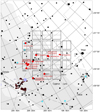 |
Fig. 1 Field of view (FoV) of the Kepler mission is respresented by the solid black squares. It is centered at RA = 19° 22 40.0, Dec = +44° 30 00.0, between the Cygnus and the Lyra constellation. The FoVs of the sixteen 3XMM-DR5 observations we analyzed (Table 1) are reported as red circles; the red numbers represent the 3XMM-DR5 unique observation ID (OBS_ID). The FoVs of some XMM-Newton observations are totally or partially overlapping. |
2.1 Spectral energy distribution (SED)
2.1.1 Multiwavelength photometry
We extracted the IR (2MASS J, H, K), optical (SLOAN g, r, i, z, Johnson U, B, V, Kepler Kp) and UV (GALEX FUV, NUV) photometry for all stars of our sample from the KIC (Brown et al. 2011). Many sources lack photometry in one or more of these bands. We excluded from the sample the KIC objects for which no 2MASS IR photometry was available (2 objects), since the wavelength range covered by 2MASS is crucial in order to perform a reliable spectral classification.
The visual inspection of the optical images via the Aladin server indicated that some stars suffer contamination from brighter objects located nearby. In such cases, even if they are recognized as distinct objects in the KIC, the photometry of the fainter one is expected to be significantly contaminated by the brighter one. Other stars suffer confusion between unresolved objects, which means that they are not resolved in the KIC survey, but can be recognized as two objects through visual inspection of the optical image. When the object was resolved in the UCAC-4 Catalog (Zacharias et al. 2012), we replaced the KIC photometry for these confused objects with the photometry provided by UCAC-4 forthe brightest one. If no UCAC-4 photometry was available, we removed the object from our sample (2 objects).
According to Pinsonneault et al. (2012), the SLOAN bands photometry reported in the KIC present a significant systematic error, as observed comparing the KIC photometry in the bands g, r, i, z with the photometry reported in the Sloan Digital Sky Survey (SDSS-DR8) in the same bands, available for ~10% of the full KIC. Pinsonneault et al. (2012) give semi-empirical formulas to correct these systematics (their Eqs. (1)–(4)). We applied these corrections to the KIC SLOAN bands photometry of all the stars of our sample. The photometry for all the stars in our sample is reported in Table A.1.
2.1.2 SED fitting
After compiling the SEDs, we fit them with photospheric BT-Settl models (Allard et al. 2012) within the Virtual Observatory SED Analyzer (VOSA, Bayo et al. 2008). The parameters of the BT-Settl models are: AV, log g, [Fe/H], and Teff. Due to parameter degeneracy it is not possible to determine all of them from the SED fit. Therefore we adopted for each star for AV, log g, and [Fe/H] values taken from the literature (see Sect. 3), leaving Teff as the only free parameter. We thus obtained, for each object, a best fit Teff under the hypothesis of a stellar model. As the uncertainty on the effective temperature we assumed the typical dispersion of the five best fit values obtained in VOSA for each object (± 200 K).
From the shape of their SED, combined with the visual inspection of the Aladin images, 16 objects were recognized as galaxies, and we removed them from our sample. The whole sample selection procedure eventually results in a sample of 125 3XMM-DR5unique sources with a reliable stellar counterpart in Kepler, with a SED that is well-fitted by a stellar photosphere model.
2.2 X-ray flux limit
The sample of stars used in the present work has been selected based on the X-ray emission observed by XMM-Newton and as such is biased towards X-ray active stars. A fundamental step in order to understand the results presented in this work is, therefore, toprovide an evaluation of the X-ray flux limit of the sample. To this end, we first produced the EPIC PN3 sensitivity map for each XMM-Newton observation of Table 1, for the energy range 0.2−2.0 keV using the task esensmap of the XMM-Newton Science Analysis Software (SAS). The sensitivity map provides in each point of the FoV the limiting count rate needed to have a 3σ detection of a point source. We measured the limiting count rate in the center of the FoV. We converted these numbers into flux sensitivity limits (fX,lim) using WebPIMMS4 assuming an APEC model with plasma temperature 0.86 keV (see Sect. 5.1.2), abundance 0.2 in solar units, and the galactic hydrogen column density provided by Kalberla et al. (2005). The resulting numbers for fX,lim are reported in the last column of Table 1. These values give an idea of the lower limit for the X-ray flux in these observations (median is  ), although wecaution that the sensitivity varies strongly (up to about one order of magnitude) from the center to the outer region of the FoV.
3 Fundamental stellar parameters
3.1 Effective temperature, visual absorption, surface gravity, and metallicity
For 119 stars out of 125 we found literature values for effective temperature (Teff), visual absorption (AV) surface gravity (log g), and metallicity ([Fe/H]) (in Huber et al. 2014 and Frasca et al. 2016). Huber et al. (2014) present a compilation of literature values for atmospheric properties (Teff, log g and [Fe/H]) derived from different observational techniques (photometry, spectroscopy, asteroseismology, and exoplanet transits), which were then homogeneously fitted to a grid of isochrones from the Dartmouth Stellar Evolution Program (DSEP; Dotter et al. 2008), for a set of ~ 200 000 stars observed by the Kepler mission in Quarters 1−16. Frasca et al. (2016) present a systematic spectroscopic study of ~50 000 Kepler stars performed using the LAMOST telescope (Zhao et al. 2012). We compared the parameters obtained by Huber et al. (2014) and Frasca et al. (2016) for our sample, in particular the effective temperatures, and we found that they agree very well within the error bars. When available, however, we preferred the values obtained from Frasca et al. (2016) through the spectroscopic analysis, since in that work the stellar parameters have been evaluated using the same method for all the stars in their sample, while Huber et al. (2014) present a collection of values obtained in several works using different techniques.
Six stars in the sample do not have Teff reported in Huber et al. (2014) or Frasca et al. (2016). For these 6 stars we adopted as Teff the effectivetemperature of the best fit of the individual SED with a model of the stellar photosphere, as described in Sect. 2.1. These stars are flagged with the “VOSA” flag in Col. 12 of Table A.2. Two out of these 6 stars have values for AV, [Fe/H] and log g in Huber et al. (2014) or Frasca et al. (2016), and we used them in the SED fit. For the others, we adopted the median values of the distribution of AV in our sample (0.38), [Fe/H]⊙ (0.0) and log g (4.0). Similarly, for the additional 15 stars that have no literature value for AV we adopted the median of 0.38 mag. The adopted values for the spectral parameters of all 125 stars are listed in Table A.2.
In order to validate our SED fitting procedure we compared the obtained Teff with the ones from the above-mentioned literature sources. The distribution of Teff and the comparison between the Teff obtained from the SED fitting and the values in the literature are reported in Fig. 2. Within the error bars, the agreement is for most stars very good, but the error bars of the values obtained by SED fitting are typically larger than the error bars in Huber et al. (2014) and especially in Frasca et al. (2016). This justifies our decision to adopt, when available, the literature values for Teff. Given the effective temperature, we assigned a spectral type to each star according to Table 5 in Pecaut & Mamajek (2013). These values are given in Table A.2.
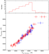 |
Fig. 2 Upper panel: distribution of the Teff of the 119 stars in our sample with Teff taken from the literature (Huber et al. 2014; Frasca et al. 2016). Lower panel: comparison between the Teff drawn from the literature and the ones obtained with the SED fitting is reported for thesame sample of stars. The colors represent the original work in which the Teff was derived.Blue: Frasca et al. (2016); red: Huber et al. (2014). |
3.2 Distance, mass, and bolometric luminosity
Figure 3 shows our stellar sample together with the DSEP isochrones on the log g vs. log Teff plane. For each star, we estimated absolute J band magnitude, mass (M) and bolometric luminosity (Lbol) by projecting its position and the related uncertainties onto the isochrones (along the vertical axis) in Fig. 3. For this task we made use of DSEP isochrones in the range of 1.0–9.5 Gyr and for each star, we selectdcd the set of isochrones corresponding to the [Fe/H] value closest to the observed value. There are a few stars the position of which on the log g vs. log Teff plane is not consistent, within the error bars, with any of the DSEP isochrones. We mark them with a flag (“DSEP outlier”) in Table A.2.
Inverting the parallaxes provided in the Gaia-DR2 (Gaia Collaboration 2018) we obtain the distances to our targets. While the overall quality of the Gaia-DR2 data is excellent, the mission is too complex to achieve optimal calibrations with less than two years of observations. As a result the Gaia-DR2 still contains many spurious astrometric solutions (Arenou et al. 2018). To remove putative problematic solutions we cleaned our dataset using the filters defined by Lindegren et al. (2018, Appendix C, Eqs. (C-1) and (C-2)). Furthermore we used additional quality indicators of the solutions (astrometric_excess_noise > 0, astrometric_gof_al > 5) to discard other potential outliers. Two stars of our sample have no Gaia parallax while the solutions for further 60 stars might not be reliable and were filtered out. For these 62 targets we derived the photometric distance from the comparison between the absolute magnitude and the observed J band magnitude. Comparison of the photometric and astrometric distances for the whole sample shows overall good agreement. For 5 targets with reliable Gaia distances we found the J band distances to have lower uncertainties. In these cases we decided to adopt the J band distances. To summarize, throughout this work we used the Gaia distances for 58 stars and the photometric J band distance for the remaining stars. Distance, mass and bolometric luminosity are reported for all 125 stars in Table A.2.
We classified the stars in our sample as main-sequence stars or giant stars according to their log g. In the log g vs. log Teff space, the stars in our sample can be separated into two groups, corresponding to the dwarf branch and to the giant branch, respectively (see Fig. 3). On this basis, we considered as main-sequence stars all the stars with log g ≥ 3.5, and as giants all the stars with log g < 3.5. With this criterion we found 19 giant stars. The four stars without log g value in the literature can not be assigned to these groups; we removed them from the sample. These stars have a flag (*) in Col. 12 of Table A.2. This work is focused on main-sequence stars. Therefore, in the following, if not differently declared, we consider only the sample of the 102 main-sequence stars. The distribution of their adopted distances is plotted in Fig. 4.
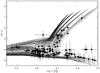 |
Fig. 3 log g −log Teff space with the set of isochrones from DSEP and the stars of our sample (black circles) overplotted. Each stack of isochrones (lines in different gray-shades) corresponds to a given value of [Fe/H] (−2.0, − 1.5, − 1.0, − 0.5, 0.0, 0.2, 0.3, 0.5 from dark to pale). |
4 Analysis of Kepler light curves
The brightness modulation in the optical light curve due to the presence of inequally distributed spots on the rotating stellar surface enables the measurement of the stellar rotation period. Rotation periods, together with several photometric activity diagnostics, have been extracted from the Kepler light curves following the procedure described by Stelzer et al. (2016). The methods developed therein for the analysis of M dwarf K2 mission lightcurves can readily be applied to the data from the main Kepler mission, and we briefly resume the steps in Sect. 4.1.
To obtain a clean sample of stars for the rotation-activity study, periods originating from mechanisms different from the rotational brightness modulation due to starspots must be identified and removed. In particular, our sample covers a broad range of Teff in the Hertzsprung–Russell diagram, including the intersection of the main-sequence with the classical instability strip, where stellar pulsations are expected. Therefore, the light curves of some stars deserve a more detailed study in order to ascertain if pulsation (but also binarity) could be the real cause of the observed variability. We performed this study by means of the Fourier decomposition (Poretti 1994) and the iterative analysis of the whole frequency spectrum (Vaníček 1971), described in Sect. 4.2.
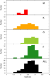 |
Fig. 4 Distribution of the adopted distances for the individual spectral types (from top to bottom: M, K, G, F) and for the whole sample of the main-sequence stars(bottom panel). |
4.1 Search for rotational periodicity
Briefly, the analysis consists of the following steps, implemented in an iterative procedure, which is described in detail by Stelzer et al. (2016): (1) period search with standard time-series analysis techniques (autocorrelation function [ACF] and Lomb–Scargle [LS] periodogram), (2) boxcar smoothing of the lightcurve and subsequent subtraction of the smoothed from the observed lightcurve, effectively removing the rotational modulation, (3) identification of “outlier” data points in the “flattened” lightcurve obtained from step (2) through σ-clipping. The outliers comprise both instrumental artefacts and flares. The latter ones are identified by imposing three criteria: (i) a threshold (3σ) for the significance of the flare data points above the flattened curve, (ii) criterion (i) applies to at least two consecutive such data points, and (iii) the maximum bin of the flare has at least a factor two higher flux than the last bin defining the flare. For a detailed description of the procedure used in each step of the analysis chain see Stelzer et al. (2016).
After the removal of the outliers we repeated the period search, but in practice the applied methods are so robust that the cleaning of the lightcurves did not alter the result. What did change after the cleaning is the amplitude of the rotation cycle, when measured between maximum and minimum flux bin. However, as we describe below in Sect. 4.4, the preferred characterization of the spot cycle amplitude involves diagnostics that are little affected by the small fraction of outlier data points. We performed this analysis for each Kepler observing Quarter independently. This allowed us to cross-check the results by comparing the periods obtained from different Quarters, as explained in Sect. 4.3.
The determination of the rotation period for a given star proceeded in the following way. We usede the routines A_CORRELATE and SCARGLE in the IDL environment5 to generate the ACF and LS periodogram. We worked independently on the ACF and LS periodogram series. For each Kepler observing Quarter, we inspected visually the ACF and LS periodogram generated by our procedure, and searched for a signal of periodic variability (a sharp peak at a certain frequency, possibly followed by the related harmonics). If absent, we rejected the Quarter from the analysis. In the ACF periodogram, we visually chose the highest peak of the series, which corresponds to the period of the modulation; this is generally the first one, or the second one if the light curve shows a double-humped pattern (as described below). In the LS periodogram, we likewise chose the highest peak.
For the majority of stars, the dominating periods derived with both techniques (ACF and LS) are consistent with each other. Deviations regard lightcurves with a double-humped shape. In this case, the light curve shows a double peak in at least some of the Kepler observing Quarters, while in others a single peak pattern may be observed. We interpret these features as the signature of two groups of spots at a roughly antipodal position on the photosphere of the star, one of which may occasionally disappear. In this case, the ACF periodogram shows generally a first peak (corresponding to half the period) that has a lower amplitude with respect to the second one, and this pattern repeats for the peaks corresponding to integer multiples of the first-peak period and of the second-peak period, respectively. In the Lomb–Scargle periodogram, the peak corresponding to the shorter period often has a larger amplitude than the longer-period peak. The interpretation of these patterns as the effect of two groups of spots on the photosphere allows us to interpret the longer period of the two, corresponding to the double of the other, as the true rotation period of the star.
We obtained for each star NQ periods, where NQ is the number of Quarters in which the star shows a periodic signal. This number varies individually for the stars of our sample, independently for the ACF and the LS method. We adopted as the star’s period the median value of the periods obtained with the ACF method from the individual quarters.
Classification of the main-sequence stars in our sample according to the type of variability observed in the Kepler light curves.
4.2 Nonrotational periodicity
For some of the stars in our sample periodic variability is identified that can not be explained with a simple spot pattern. In such cases the Fourier decomposition and the evaluation of the whole frequency spectra were very helpful. The frequency spectra of the genuine spotted stars are characterized by the harmonics of the rotational period and by low-frequency peaks due to the activity and rotational cycle-to-cycle period variations due to the shift in the spots’ latitude and to stellar differential rotation, and by some rotational cycle-to-cycle variation in the shape and amplitude of the lightcurve due to the variation of the area and shape of starspots. Other kinds of periodicity present different patterns.
We performed a dedicated anlysis of the light curves of the stars that do not show a clear variability pattern in order to classify their nonrotational variability. We found one multiperiodic star showing the high-frequency pulsational regime of δ Sct stars and three multiperiodic stars showing the low-frequency regime of γ Dor stars. In thelight curves of two stars the amplitudes of the even Fourier harmonics are much larger than those of the odd ones, as necessary tofit both the sharp minima and the large maxima shown by contact binaries. For three stars it remains ambiguous if the variability is due to star spots or due to orbital motion in a contact binary; another two stars display non-periodic variability that we could not classify. Finally, five stars are likely rotational variables but displaying more than one period possibly indicating a binary composed of two spotted stars or a complex pattern with uncertain period. We removed these 16 stars from the sample considered for the rotation-activity relation. A summary of the number of main-sequence stars in each variability class for spectral type is given in Table 2.
4.3 Finalsample of spotted stars
From the analysis described above, we can derive a rotation period for 74 stars in our sample, meaning that these stars are inhomogeneously spotted. For the subsequent analysis, we also computed the Rossby number, defined as R0 = Prot∕τconv, that is the ratio between the rotation period and the convective turnover time. The convective turnover time is the characteristic time of circulation within a convective cell in the stellar sub-photosphere, and not directly observable. We calculated it from Teff using Eq. (36) in Cranmer & Saar (2011), which is valid in the range 3300 K ≲ Teff ≲ 7000 K. All but two of the stars in our sample are within this range of Teff. The rotation periods and Rossby numbers for all “spotted” stars are listed in Table A.3. Our subsequent photometric variability analysis is limited to this sample.
4.4 Photometric activity diagnostics
From the analysis of the Kepler light curves we also obtained various diagnostics for the stellar photospheric activity: the light curve amplitude and the standard deviation of the light curve. The light curve amplitude is the photometric difference between the maximum and the minimum of the rotationally-modulated light curve, determined (in a light curve cleaned from flares) by the contrast between spotted and unspotted photosphere, combined with the inhomogeneous distribution of spots which causes the spot coverage of the observed stellar hemisphere to vary during the rotation. Analogous to Stelzer et al. (2016) and for consistency with the previous literature we decided to define the spot cycle amplitude as the range between the 5th and 95th percentile of the observed flux values in a single rotation cycle (Rvar, see Basri et al. 2013), and we adopt the modified definition of Rvar introduced by McQuillan et al. (2013), Rper, which is the mean of the Rvar values measured individually on all observed rotation cycles, expressed in percent. Cutting the upper- and lower-most 5% of the data points is another way of removing the outliers, such that no difference between the Rvar values obtained from the original light curve with the 5th and 95th percentile and from the cleaned lightcurve is expected. We verified this by comparing the Rvar values extracted from the light curves cleaned from flares and outliers and the Rvar values obtained from the original light curves.
The second activity diagnostic extracted from Kepler light curves that we use to characterize the variability during the spot cycle is the standard deviation of the whole light curve (Sph), and the average of the standard deviations computed for time intervals k × Prot, with k integer, first defined by Mathur et al. (2014a). Mathur et al. (2014a) have shown for a sample of 22 stars that roughly after five rotation cycles the full range of flux variation is reached. Therefore, we computed Sph and ⟨Sph,k=5⟩ for the stars in our sample. The standard deviation of the light curve is used as a proxy of magnetic activity also by He et al. (2015), in a study on the activity of two solar-like Kepler stars.
Finally,we computed the standard deviation of the flattened light curves (Sflat), measured on the light curves cleaned from flares and outliers, and from which the rotational cycle has been removed (see description at the beginning of this section). Stelzer et al. (2016) have established this parameter as an indicator for low-level unresolved astrophysical variability such as small unresolved flares and/or small and fast-changing spots for their sample of nearby M dwarfs observed in the K2 mission.
All these photometric activity diagnostics are listed in Table A.3. It is worth noting here that the noise level in the flattened lightcurve is expected to depend on the brightness of the star. In fact, Fig. 5 shows a correlation between the Kepler magnitude and Sflat. As can be seen in Fig. 5, the apparent brightness of our sample stars is on average larger for earlier spectral types. As a consequence, the noise tends to be smaller in those stars. This must be taken into account in the analysis of other kinds of variability; see e.g. Sect. 6.3.
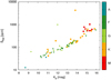 |
Fig. 5 Standard deviation of the flattened lightcurve (Sflat) vs. Kepler magnitude. Shown is for each star the minimum of Sflat from all quarters of observation. |
5 X-ray and UV activity
As our sample is X-ray selected, every star in the sample has an associated X-ray detection. In the main-sequence sample, 36 stars have also been detected in one or both of the UV energy bands (Near Ultra-Violet, NUV, and Far Ultra-Violet, FUV) of GALEX. In this section we analyze the X-ray and UV luminosity, and the corresponding activity indexes, defined as the ratio between the luminosity in the high-energy band and the bolometric luminosity of the star, as indicators of the stellar magnetic activity.
5.1 X-ray data analysis
5.1.1 Source X-ray luminosity
We calculated the X-ray luminosity of each star in the sample in the energy band 0.2−2.0 keV (“soft” energy band, 3XMM-DR5 catalog energy band 6). This range of energies corresponds approximately to the energy bands used in previous studies of the rotation-activity connection that were mainly based upon ROSAT data (e.g., Wright et al. 2011).
In the 3XMM-DR5 catalog, there are many objects (“sources”) that have been observed more than once: so, for a certain source, there can be many detections. Each row of the catalog – which represents an individual detection of a certain source – contains a set of parameters referred to the detection itself, and a set of parameters averaged on all the detections available forthat source. The catalog provides the fluxes expected for a power law emission model for both the detections and the source. However, the power law model, to which the fluxes given in 3XMM-DR5 refer, is not appropriate for describing the X-ray emission of late-type stars. Therefore, we re-calculated the X-ray flux in the bands 0.2−2.0 keV from the EPIC PN count rate (or the MOS, if PN is not available), using the HEASARC online tool WebPIMMS, in which we assume for the X-ray emission of the stars a thermal APEC model (Smith et al. 2001). 3XMM-DR5 gives the detection count rate for each of the three EPIC (European Photon Imaging Camera) instruments (PN, MOS1 and MOS2) on board the XMM-Newton mission, and the associated uncertainty, but it does not give the source count rate. As described above, the detection count rate is different from the source count rate when the source has multiple detections in the catalog. This happens for 11 sources in our sample. So, we calculated the X-ray flux for these objects rescaling one of the individual detection count rate for the factor
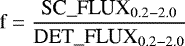 (1)
(1)
where SC_FLUX0.2−2.0 and DET_FLUX0.2−2.0 are respectively the “source” and “detection” flux provided by 3XMM-DR5.
The APEC model in WebPIMMS requires as input parameters the hydrogen column density (NH), the metallicity and the temperature of the emitting plasma. We estimated the hydrogen column density for each source from the visual absorption AV following Cardelli et al. (1989), as
 (2)
(2)
We adopted an average abundance of 0.2 in solar units, which is a typical value for the coronae of X-ray emitting late-type stars (see e.g. Pandey & Singh 2012). We calculated the count-to-flux conversion factor with WebPIMMS. To establish an operational kT, we fit the spectra of the brightest X-ray sources in XSPEC, and assumed for all stars the kT value in the WebPIMMS grid (kT = 0.86 keV) which is closest to the average kT obtained from the spectral fits (kT = 0.83 keV). The spectral analysis of the brightest sources is described in the following.
Best fit spectral parameters for the 17 brightest X-ray sources (more than 200 counts) identified as rotational variables; parameters are for a phabs*apec or phabs*(apec+apec) model.
5.1.2 Spectral analysis
We selectedthe subsample of stars for which there are at least 200 events in the source extraction region in the three EPIC instruments together (PN+MOS1+MOS2). Excluding the stars classified as eclipsing or contact binaries, the sample consists of 19 stars. For each one, we extracted the source and background spectrum in the energy band 0.3−10.0 keV, and performed a joint spectral analysis with XSPEC 12.8.1 (Arnaud 1996) of the spectra of all EPIC instruments available forthat source. We fit the spectra with an absorbed one-temperature APEC model (phabs*apec) or an absorbed two-temperature APEC model (phabs*(apec+apec)). We set the coronal abundance to the typical value of 0.2 in solar units (see above) to reduce the number of free parameters and avoid degeneracy.
Two stars showed a significant parameter degeneracy in their spectrum, so we removed them from the analysis. For the stars for which the model requires two temperatures, we calculated an average temperatureweighted on the flux of the two APEC components. The results of the best fit for each of the 17 stars, all characterized by a null-hypothesis probability >0.3%, are reported in Table 3. We calculated the average kT over the 17 stars (⟨kT⟩ = 0.83 keV).
With the parameters given in Sect. 5.1.1, we obtained from WebPIMMS the expected flux for each source.We then compared these fluxes with the fluxes obtained from the spectral analysis, for each of the 17 sources for which the spectral fit in XSPEC was performed. For each of these stars we calculated the ratio between the XSPEC fluxand the flux from WebPIMMS. For PN, MOS1 and MOS2, we found an average ratio of respectively 0.91, 0.89, 1.00 in the soft energy band 0.2−2.0 keV. We corrected the fluxes obtained with WebPIMMS for the faint (<200 counts) sources by multiplying them with this factor. This correction is meant to obtain from WebPIMMS a flux that is, on average, as close as possible to the actual flux obtained from a spectral fit.
In the sample of 17 bright stars, kT ranges from 0.49 to 1.3 keV. This range is typical for active stars, and the actual plasma temperatures of the bulk of the faint stars is likely in the same range. This span of temperatures introduces an error in the flux calculated with the average kT, allowing fluxes which are up to ~2% lower or ~15% higher than the one calculated from the average temperature of the bright stars. If the 17 X-ray-brightest sources are not representative of our whole sample, these errors may be somewhat larger for the faint stars.
From the corrected fluxes we calculated the X-ray luminosity using the distances derived in Sect. 3.2. For each source we calculated the X-ray activity index as
 (3)
(3)
The distributions of the X-ray luminosity and of the corresponding activity index in the soft energy band (0.2−2.0 keV) are reportedin Fig. 6. The individual X-ray luminosities are listed in Table A.4.
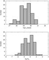 |
Fig. 6 Distribution of the X-ray luminosity and of the X-ray activity index in the energy band 0.2–2.0 keV for the 102 main-sequence stars. |
5.1.3 Considerations on the X-ray luminosity distribution
We compared the distribution of the X-ray luminosity in the range 0.2−2.0 keV for the starsin our sample with those in the NEXXUS sample of Schmitt & Liefke (2004), which consists in a compilation of coronal X-ray emission for nearby late-type stars based on the ROSAT observatory. The distribution of the X-ray luminosity for our main-sequence sample and for the one from Schmitt & Liefke (2004) is plotted, for each spectral type and forthe whole sample, in Fig. 7.
To first order we consider NEXXUS as a volume-limited sample of nearby stars, representing the full range of X-ray activity of the solar-like stellar population. Note, however, that Stelzer et al. (2013) show that even in as small a volume as 10 pc around the Sun about 40% of the M dwarfs have no X-ray detection in the RASS. From the comparison with our distribution, it is evident that our sample presents a significant bias towards high X-ray luminosities most marked for the latest spectral types reflecting the mass (or Teff) dependence of X-ray luminosity. The stars in our sample, which is flux-limited, are on average at a much greater distance (see Fig. 7, median distance for the whole sample: ~ 500 pc). Therefore, we interpret the bias of our sample towards active stars as due to both the X-ray selection and the large distances.
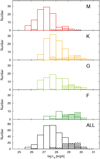 |
Fig. 7 Distribution of the X-ray luminosity in the energy band 0.2–2.0 keV, for the 102 main-sequence stars of the Kepler - XMM-Newton sample (hatched histograms) and for the NEXXUS stars from Schmitt & Liefke (2004) (solid line) for each spectral type class separately and for all spectral types combined. |
5.1.4 X-ray light curves
In order to study the variability of the X-ray emission and to search for X-ray flares, we analyzed the light curves provided by the EXTraS (Exploring the X-ray Transient and variable Sky) project6 (De Luca et al. 2016). EXTraS was synchronized with 3XMM-DR4, while we are studying X-ray sources from 3XMM-DR5 in the Kepler field. Therefore, light curves for observations 0671230201 and 0671230601 are not present in the public EXTraS database, but were produced for this work by the EXTraS team, using the EXTraS analysis pipeline.
EXTraS provides a set of uniform bin light curves with different bin size, from 10 s up to 5000 s and an optimum bin size (chosen to have at least 25 counts in each bin), both for the source and the background extraction regions. In addition, EXTraS also provides light curves produced via an adaptive binning, namely Bayesian blocks (Scargle et al. 2013) algorithm for each source and for the related background region. This algorithm starts with an initial set of cells defined on the basis of the number of events in the source and background region, and provides a final set of different-duration bins, each of which has a count rate that is not consistent, within 3σ, with the count rate of the adjacent bins.
In the EXTraS analysis pipeline, all the source light curves, both the ones obtained with the uniform bin algorithm and the Bayesian blocks algorithm, are automatically fitted with a series of different models that account for simple variability patterns (constant, linear, quadratic, negative exponential, constant plus flare, constant plus eclipse). This is a standard algorithm that is part of the EXTraS pipeline, and it is applied to all the light curves in the same way. Its purpose is to provide a first-step indication of the kinds of variability possibly present in the light curve, and not to perform a detailed modeling of the variability features observed, nor to determine their parameters. All results are in the database, and online searches can be performed with the query form.
5.1.5 X-ray flaring
For each X-ray source in our sample, we searched for X-ray flares in the EXTraS light curves. First, we inspected the results of the fit performed on the light curves with different variability models by the EXTraS pipeline. As stated above, these results can be used for a first assessment for the kind of variability present in the light curve. If at least one among the uniform bin or adaptive bin light curves is better fitted by a constant plus flare model (higher null-hypothesis probability) than the other models, this is a good indication of a possible flare. This flare model consists of a constant flux level over which a simple flare profile is superimposed, that is a steep linear flux increase, followed by an exponential decay.
The Bayesian blocks light curves are particularly useful to detect flares, which appear as one or more blocks that show a higher flux than the preceeding and following blocks. If the flare occurred at the beginning or at the end of the observation, the Bayesian blocks light curve may show only the rise phase or the decay phase. In this case, we rely on the uniform bin light curves to establish if the event is a true flare or not. We also require that the flare was observed in at least two of the EPIC instruments. The visual inspection of the light curves is however crucial in order to recognize genuine flares, so we inspect all the available EXTraS light curves for each star in our sample.
With this procedure, based on the EXTraS pipeline products we detected 6 X-ray flares on 5 stars, and by visual inspection we identified an additional likely flare on a sixth star, KIC 7018131 (Figs. 8, and 9). In view of the low count statistics of the X-ray lightcurves some remarks on the individual events are in order. KIC 9048976 shows two possible flares: the Bayesian blocks algorithm shows one block with a higher flux at the beginning and at the end of the light curve, impeding the observation of the full flare profile. KIC 8909598 also shows an X-ray flare at the end of the observation. The uniform bin light curves reveal a quite obvious flare profile both in PN and MOS2 cameras. However, this star does not have a reliable main-sequence classification (unknown log g), so we do not consider it in the analysis. For KIC 9048551 the Bayesian block algorithm identifies one flare event, but the uniform bin lightcurve shows evidence of substructure contemporaneous with two events seen in the Kepler band.
The X-ray flares shown in Fig. 8 have simultanous white-light flares in the Kepler light curves (see Sect. 6.3). Figure 9 displays the light curves for the X-ray flares without a simultaneous white-light counterpart revealed with the flare detection algorithm described in Sect. 4.1. Evidence for a weak increase of the optical brightness at times of the X-ray flare is, however, seen in all the contemporaneous Kepler lightcurves.
In Table 4 we report the start time of the X-ray flares (Col. 2), according to the Bayesian blocks light curve except for KIC 7018131, for which we infer the start time from the 500 s uniform bin light curve of EPIC/pn, since the Bayesian blocks light curve has only one block. We also report the quiescent (Col. 3) and peak (Col. 4) X-ray count rate, taken from the 500 s uniform bin light curve of EPIC/pn, together with the overall number of white-light flares observed in the whole Kepler light curve for the star (Col. 5), its white-light flare frequency (Col. 6), the average, maximum and minimum peak amplitude of the Kepler flares (Apeak, photometric ratio between the peak bin and the baseline of the flare, Cols. 7 and 8). This parameter is discussed in more detail in Sect. 6.3.1.
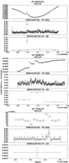 |
Fig. 8 Simultaneous Kepler and XMM-Newton EPIC PN light curves for the stars showing a simultaneous X-ray andwhite-light flare. The EPIC light curves produced by the EXTraS pipeline with 500 s uniform binning and with the Bayesian blocks adaptive binning are plotted. The flare in the Kepler light curve of KIC 7018131 corresponds to a bump in the EPIC uniform bin lightcurve which is, however, not significant at a 3σ level over the baseline, and not detected with the Bayesian block algorithm. |
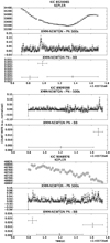 |
Fig. 9 XMM-Newton EPIC PN light curves for the X-ray flares without a white-light counterpart detected by our flare-detection algorithm. Simultaneous Kepler light curves are not available for KIC 8909598. |
5.2 UV activity
The KIC provides UV magnitudes obtained with the Galaxy Evolution Explorer (GALEX). The GALEX satellite performed imaging in two UV bands, far-UV (henceforth FUV; λeff= 1516 Å, Δλ = 268 Å, and near-UV (henceforth NUV; λeff = 2267 Å, Δλ = 732 Å). The KIC gives a NUV detection for 71 stars from our main-sequence sample (i.e., 70%) and a FUV detection for 20 main-sequence stars (20%). All but one of the stars with a FUV detection also have a NUV detection. The individual values for the observed NUV and FUV luminosities are listed in Cols. 3 and 4 of Table A.4.
The SED fit provides UV fluxes for the stellar photosphere. In order to validate these measurements, we converted the NUV de-absorbed photospheric fluxes obtained from VOSA into absolute magnitudes and compared the relation between these magnitudes and the B−V color (derived from Pecaut & Mamajek 2013) with the analogous relation observed for a set of photospheric NUV magnitudes provided by Findeisen et al. (2011) in their Table 1. Figure 10 shows that our values are in good agreement with the ones of Findeisen et al. (2011).
For some stars in our sample the observed GALEX NUV and FUV fluxes are significantly higher than the prediction of the best-fitting photosphere model. This UV excess, that is the positive difference between the observed UV flux (fUV,obs) and the photospheric flux of the BT-Settl model in the same UV band (fUV,ph) represents the UV emission associated with magnetic activity processes in the stellar chromosphere. Following Stelzer et al. (2013), we calculated the corresponding UV activity index as
 (4)
(4)
where fUV,exc is the UV excess flux attributed to activity, and fbol is the bolometric flux. The bolometric flux is obtained from interpolation on the DSEP isochrones, as described in Sect. 3.
We calculated the UV excess in both the GALEX FUV and NUV band, where available. After trying different values and visually inspecting the SED, we found that a threshold of 13% on the ratio between the excess flux and the photospheric expected flux was the best choice to select the stars with a true UV excess. We found 45 main-sequence stars with a NUV excess, ten of them display also a FUV excess, and an additional 4 have a FUV excess but no NUV excess. The NUV and FUV excess luminosities are provided in Cols. 5 and 6 of Table A.4.
6 Results and discussion
6.1 Rotation periods
For 74 main-sequence stars out of 102 (73%) the Kepler light curve is dominated by the rotational brightness modulation due to starspots, with a period in the explored range Prot < 90 d. For the individual spectral types, the fraction of main-sequence stars with a rotational brightness modulation is: A 66% (2/3), F 65% (24/37), G 73% (19/26), K 75% (21/28) and M 100% (8/8). Our period detection rate is higher with respect to other studies based on Kepler data (McQuillan et al. 2013, 2014, 37% in the range 3500 K < Teff < 6500 K, F ~27%, G ~25%, K ~60%, M ~80%; Stelzer et al. 2016, 73% for M dwarfs). This is probably an effect of the selection bias towards active (and thus strongly spotted) stars as well as the removal of giant stars from our sample.
In Table 2 a summary of the number of stars with rotation period from our analysis is reported for every spectral type, together with the number of stars with other types of brightness modulation patterns. We refer to Table A.2 for the classification of the photometric variability for each star in the sample.
Only 54 stars out of 74 have previously reported periods from McQuillan et al. (2014), obtained from the same Kepler light curves. For the 54 stars for which a rotation period is reported in McQuillan et al. (2014), those periods are consistent with our values within uncertainties. The remaining 20 stars do not have any previously determined period in the literature.
Parameters of the X-ray flares and Kepler flare characteristic of the X-ray flaring stars.
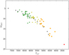 |
Fig. 10 Absolute NUV magnitude versus Johnson color B–V for the stars in our sample with a GALEX NUV detection, for each spectral type, and for the values of Table 1 in Findeisen et al. (2011) (black dots). Different symbols represent the spectral type; red circles: M, orange squares: K, light-green triangle up: G, dark-green triangle down: F. |
6.2 Activity-rotation relation
In Fig. 11, we present the relation between the X-ray luminosity in the soft energy band 0.2−2.0 keV and the rotation period, together with the relation between the X-ray activity index (defined in Eq. (3)) and the Rossby number. A clear decrease in X-ray activity levels is observed for slower rotators. This effect is more evident in the AIx versus Rossby number plot, and produces a “kink” in the distribution, which can be seen quite clearly in the overall sample of all stars, and also in the subsamples of K stars, while for M, G and F stars it is not obvious as these subsamples comprise only a limited range of rotation rates. The “kink” suggests the presence of a correlated regime for slow rotators, and of a saturated regime for fast rotators, with a separation occurring at ~ 8 d (from visual inspection). The wide range of LX and AIX independent of Prot for the (generally fast rotating) F stars is remarkable: it is possible that the F stars present a decoupling between rotation and activity because of their shallow convective zones. This group may also include active binary stars (RS CVn) with unknown contribution to the X-ray emission from the cool companions.
In Fig. 11 we show for comparison the literature compilation from Wright et al. (2011) and the previous empirical relations obtained by Pizzolato et al. (2003) based on a small sample with mostly spectroscopic rotation measurements (solid lines). The rotation periods in Wright et al. (2011) were collected from several works which use both spectroscopic and photometric techniques, and the X-ray fluxes were obtained from the analysis of data taken from different missions, such as XMM-Newton and ROSAT. We find excellent agreement of our more homogeneous data with that study. Especially, the scatter clearly decreases when X-ray luminosity and rotation period are replaced by AIx and R0, respectively.Contrary to previous work where no uncertainties were estimated, we present here conservative error bars for our sample. These are dominated by the uncertainties in the distances of stars without Gaia parallax that are derived from mapping the stars in the log g − log Teff diagram onto the Dartmouth isochrones (see Sect. 3.2), meaning that they ultimately go back to the uncertainties in the spectroscopic parameters.
The rotation-activity relation of M dwarfs in our sample can be compared to that of M dwarfs observed in the K2 mission studied by Stelzer et al. (2016) with an analogous approach. In Fig. 12 we show the Lx − Prot relation for the two samples. Our X-ray selection evidently excludes slowly rotating M stars in the non-saturated regime. This can also be seenfrom the comparison with the bimodal relation suggested by Pizzolato et al. (2003) (solid black line in Fig. 11) which is, however, itself extremely poorly defined. Recent M dwarf studies by Wright & Drake (2016) and Wright et al. (2018), also shown in the figure, used rotation periods measured with ground-based instruments. They cover the long-period “correlated” region and are complementary to our Kepler study.
The scatter observed in the saturated regime of LX and AIx for M stars of given Prot is large but consistent with that observed by Wright et al. (2011), Pizzolato et al. (2003) and Stelzer et al. (2016), and probably due, at least in part, to the spectral type distribution within the M class, with cooler stars having lower X-ray luminosity. The scatter decreases when considering the relation AIx versus R0. Because of the relatively low statistics in our sample, in particular the low number of stars in the correlated regime, it would be difficult to establish with good confidence the turnover point between the correlated and saturated regime, nor the slope of the correlated part of the relation.
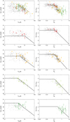 |
Fig. 11 X-ray activity versus rotation for the full sample, M-, K-, G-, and F-type stars (from top to bottom). Left panels: X-ray luminosity in the energy band 0.2− 2.0 keV versus Kepler Prot. Right panels: X-ray activity index versus Rossby number. Colours and symbols follow the convention defined in Fig. 10. The stars in the sample of Wright et al. (2011) are shown as small black dots. The solid lines represent the best-fit relations between X-ray emission and rotation period found by Pizzolato et al. (2003) for stellar mass ranges corresponding approximately to spectral types. |
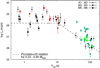 |
Fig. 12 LX vs. Prot for M dwarfs: red – this work, black – K2 sample from Stelzer et al. (2016) (their Fig. 15), green – stars published by Wright & Drake (2016) and Wright et al. (2018). The solid line represents the best-fit rotation-activity relation from Pizzolato et al. (2003) in the range 0.22–0.60 M⊙. |
6.3 Kepler activity diagnostics
6.3.1 Optical flares
We explore here the optical flaring activity measured in the Kepler lightcurves of the spotted stars. This analysis must consider that the sensitivity for detecting flares depends on the (quiescent) brightness of the star and is different for each star. The criteria in our definition of flare include a ≥3σ upward deviation from the flattened lightcurve (see Sect. 4.1). As a result of the relation between Kp and spectral type in our sample (evident in Fig. 5), the minimum measurable flare amplitude (Apeak) – defined here as the relative brightness difference between the flare peak and the flattened lightcurve – shows a trend with spectral type (Fig. 13).
For a meaningful comparison of our sample which covers a large range in brightness we must convert relative quantities, such as Apeak and Sflat, to absolute ones. The Kepler photometry is not flux calibrated. However, an approximate brightness can be associated to the flattened lightcurve assuming that this normalized “quiescent” emission corresponds to the Kepler magnitude of the star. We convert Kp to flux using the zero-point and effective bandwidth provided at the filter profile service of the Spanish Virtual Observatory (SVO)7. Then we apply the distances derived in Sect. 3.2 to obtain the “quiescent” luminosity in the Kepler band,  . Similarly, the flare amplitude is converted from its relative value (Apeak) to a luminosity,
  . The resulting relation between flare amplitude (in erg s−1) and quiescent luminosity is shown in Fig. 14. The lower envelope is defined by our flare detection threshold which is marked as a horizontal bar for each star and which is rising with increasing stellar luminosity. The A-type stars form an exception to this trend. They show lower flare amplitudes than expected for their
  . This finding can easily be explained when the observed flares are attributed to unknown and unresolved later-type companion stars. In this scenario the actual
  value of the flare-host would be lower making the true amplitude
  higher than measured. This would shift the data points to the left and upwards in Fig. 14.
For a given star, the range of flare luminosities,  extends up to ~2 orders of magnitude above the amplitude of the minimum observable flare. The range of flare amplitudes is smaller for G and F stars but this is probably related to the lack of sensitivity for the detection of low-luminosity flares. This is evident from consideration of the Sflat values which set the detection threshold (see Figs. 13 and 14).
One of the aims of our study is the investigation of a connection between flaring activity and rotation rate. In their analogous study on M dwarfsobserved in the K2 mission, Stelzer et al. (2016) have found a sharp transition in the optical flaring behavior at a period of ~ 10 d. This transition is difficult to probe with this X-ray selected Kepler sample for two reasons: (1) the small number of slow rotators and (2) the broad range of Kp translating into a dishomogeneous flare detection threshold. If we restrict our sample to M dwarfs which span a relatively narrow range in optical brightness (cf. Fig. 5), the relative flare amplitudes and the flare frequencies are consistent with the results obtained by Stelzer et al. (2016) but we are covering only the fast periods up to the presumed transition (see Fig. 15). The average flare frequency of the M stars in our sample (0.12 flares d−1) is in excellent agreement with the average flare frequency in Stelzer et al. (2016) calculated over the Prot range (Prot ≲ 10 d) covered by the Kepler M stars (0.11 flares d−1). This shows that our Kepler sample, albeit highly incomplete at the slow-rotation and low-activity side, is representative for fast rotating and active M dwarfs.
Analogous to the study of Stelzer et al. (2016) on K2 lightcurves, the sampling time of 29.4 min of the Kepler lightcurves used in this work, together with the characteristics of the flare search algorithm (see Sect. 4.3), prevent the detection of flares with duration below ~ 1 h. As a consequence, we detect mostly flares with large-amplitude and relatively long duration. It can be suspected that there is a significant population of smaller and shorter flares that cannot be observed, due to the long cadence of the light curves and to the flare-extraction pipeline. Therefore, the flare frequencies of Fig. 15 and Table 5 likely represent a lower limit to the actual values.
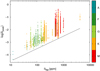 |
Fig. 13 Relative peak amplitudes of all detected optical flares in the Kepler lightcurves measured with respect to the flattened lightcurve. The gray line denotes our threshold for flare detection set to 3 × Sflat. |
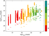 |
Fig. 14 Absolute flare amplitudes versus quiescent luminosity represented by the Kepler magnitude associated with the flattened lightcurve; see text for details. |
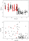 |
Fig. 15 Relative flare amplitudes (Apeak; top panel) and flare frequency (bottom panel) versus rotation period for the M stars in our Kepler sample (red) and for the M stars of the K2 sample presented by Stelzer et al. (2016) (black). |
Mean values and standard deviations measured for photometric activity diagnostics in the Kepler/XMM-Newton sample.
6.3.2 X-ray versus white-light flares
As described in Sect. 5.1.5 we find seven X-ray flares on six stars. For these events the count rate at the flare peak (as measured from the EXTraS Bayesian light curves) is a factor 3− 7 higher than during the non-flaring, quiescent time-intervals. As a result of the large distances of the Kepler stars, the X-ray count rates are small and the low counts statistics prevent a detailed quantitative analysis such as the determination of decay time and total flare energy.
All the stars with an X-ray flare except KIC 8909598 are classified as main-sequence: one M-type, three K-type and one F-type star. We do not consider KIC 8909598 in the further analysis. All but the F star (KIC 8520065), show a clearrotational modulation in their Kepler light curves. This latter one is according to our analysis probably also a rotator, but the variability pattern is unclear, and it is not possible to estimate a reliable rotation period.
We compare the X-ray flaring with the white-light flaring activity. Of the four stars with a detected rotation period, three show a largenumber of white-light flares in the Kepler lightcurves, and are among the stars with the highest optical flare frequency. This underlines the strong connection between X-ray and optical flaring mechanism: since the X-ray observationsare relatively short in duration, X-ray flares are observed predominantly in the light curves of the stars which show a higher optical flare frequency. There are simultaneous XMM-Newton/Kepler observations for 69 stars in our sample. All the X-ray flaring stars in our sample (except for KIC 8909598, which, as mentioned, we exclude from the analysis) have a Kepler observation simultaneous with the XMM-Newton observation in which theX-ray flare was detected. No white-light flares without X-ray counterpart were detected during the simultaneous X-ray and white-light observations.
Our automated Kepler flare-detection algorithm finds 3 events occurring within ~1 h from the observed X-ray flares (see Fig. 8). However, visual inspection shows that the other X-ray flares likely have optical counterparts as well, which have remained below the detection threshold of our automatic algorithm. Finally, a simultaneous event, detected only by visual inspection of the X-ray (and Kepler) lightcurves, occurred on one star. To summarize, of the 6 X-ray flares observed from rotating dwarf stars, there is evidence for a contemporaneous optical event in all cases, but only for three of them is the associated white-light flare clearly detected (one M-type and two K-type stars).
6.3.3 Other Kepler activity diagnostics
Here we examine the distribution of the photospheric activity diagnostics Sph and Rper (see Sect. 4.4 for their definition). As mentioned above, as a result of the bias to active stars, our Kepler sample does not allow us to study the transition of the optical activity diagnostics at Prot ~ 10 d revealed in the K2 data of nearby M dwarfs. Figure 16 shows our M dwarf sample compared to the one studied by Stelzer et al. (2016). Similar to the results on optical flares, the rotation cycle amplitude (Rper) and the overall variability of the lightcurve (Sph) of the two samples follow the same distribution in the fast-rotator regime.
We can examine the spectral type dependence of the photometric activity diagnostics, provided that – analogous to the detection of flares – the brightness dependence of the sensitivity for measuring variations is considered. In Fig. 17 we display Sph and Rper, versus Kp separately for each spectral class. The average values of Sph and Rper for each spectral type are listed in Table 5. While the exclusively high values for the activity diagnostics in the M dwarfs may be due to their faintness, preventing the detection of small variations, a curious distinction is seen for F stars. Albeit covering roughly the same level of (quiescent) brightness in the Kepler band as the G dwarfs and some of the K dwarfs and the same range of Prot (see e.g. Fig. 11), the variability of the F stars is markedly smaller. This points at intrinsically weaker variability in F stars. A similar effect is seen in Fig. 4 of McQuillan et al. (2014). Our finding is aggravated by the fact that the F stars of our sample are more active, that is have higher Sph values, than a sample of 22 F stars selected from the Kepler Asteroseismic Science Consortium (KASC) programme studied by Mathur et al. (2014b).
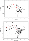 |
Fig. 16 Photometric activity diagnostics versus rotation period for M stars. Red dots – M stars in our sample; black dots – K2 M dwarf sample of Stelzer et al. (2016); gray dots – field M dwarfs in the sample by Mathur et al. (2014a) in the top panel and field M dwarfs from McQuillan et al. (2013) in the bottom panel. |
6.4 UV activity
As this sample is X-ray selected, all stars for which we detected an UV excess have an X-ray detection. We show in Fig. 18 the correlation between the UV excess luminosity (as calculated in Sect. 5.2) and the X-ray luminosity. With the caveat that the GALEX filters exclude some important chromospheric contributions, most notably the Mg II doublet, these relations represent a comparison of the chromospheric and the coronal radiative energy output. The sample with FUV excess is too small for any conclusion. We perform the Spearman’s and Kendall’s correlation tests for the NUV and X-ray luminosities of each SpT and find that only the K stars show a significant positive correlation between the two luminosities (p-values < 0.05) with rank correlation coefficients ρs = 0.85 and ρK = 0.64. The F and G stars show each a considerable spread in the distribution, similar to the behavior of the F stars in the X-ray-rotation relation of Fig. 11.
We also compare the UV emission levels of our sample to the UV emission of the exoplanet hosts studied by Shkolnik (2013). Deviating from the remainder of this paper, which is focused on the high-energy emission due to stellar activity, we consider here the total observed UV emission which includes photospheric plus chromospheric contribution. This enables a direct comparison to the work of Shkolnik (2013). Secondly, for the irradiation of exoplanets the relevant parameter is the total UV output of the star irrespective of its origin. Figure 19 shows the distribution of LNUV ∕ Lbol versus Teff for our stars and for the sample of exoplanet hosts analyzed by Shkolnik (2013). Our UV luminosity values are for given Teff about one order of magnitude above the values of the stars with exoplanets. This might be explained by an oppositely directed bias in both samples: While our sample is biased towards active stars, known exoplanet hosts are typically inactive as a result of the selection criteria for planet search programs. A second reason that might influence the differences between the NUV emission of the two samples is the fact that the stars in the sample of Shkolnik (2013) are typically nearby (tens of parsec), such that many stars were saturated in the GALEX observations and they have been removed from the analysis, thus generating a bias towards small NUV luminosity. Based on these arguments, there is good reason to believe that the two samples taken together represent the full range of NUV luminosity for each spectral type.
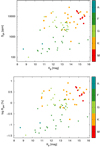 |
Fig. 17 Photometric activity diagnostics versus Kepler magnitude for the stars in our Kepler/XMM-Newton sample divided in spectral type bins. Top: Sph versus Kepler magnitude; Bottom: log Rper versus Kepler magnitude. |
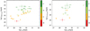 |
Fig. 18 UV chromospheric excess luminosity versus X-ray luminosity for the full sample. |
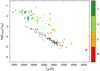 |
Fig. 19 Observed fractional NUV luminosity versus Teff for the starsin our sample (with the usual color code) and the ones from Shkolnik (2013, black dots). |
6.5 A-type stars
Three stars in our sample are classified as A-type on the basis of their effective temperature. The light curve of one of them (KIC 5113797) shows a variability pattern that suggests an association with the class of γ Dor non-radial pulsators. The others (KIC 8703413, KIC 9048114) have a clear rotational modulation pattern suggesting the presence of star spots. Only 3 flares have been detected by our algorithm in the Kepler lightcurves of the A stars in our sample.
Late A-type stars represent the high-mass borderline of the magnetically active stars. A change in the stellar structure occurs with respect to later-type stars: the outer convective layer disappears, leaving a fully radiative stellar interior. It is generally believed that the standard stellar dynamo model can not be applied to fully radiative stars, which lack the transition between convective and radiative zones. Dynamos may operate in the small convective cores of hot stars, but a major problem is the emergence of the ensuing fields to the surface of the stars where magnetic activity is observed. Considering these difficulties, the magnetic activity apparently observed on A-type stars, and especially the X-ray emission, is often ascribed to unresolved late-type companion stars in binary systems. In a systematic study of a large sample of A-type stars associated with a ROSAT X-ray source about 25% are bona-fide single stars (Schröder & Schmitt 2007), and the question on whether A-type stars can maintain a corona has not been conclusively resolved.
Similarly, the occurrence of photospheric magnetic activity in A-type stars is disputed. Balona (2013, 2015) performed a search for activity in the A stars observed by Kepler. Both rotational variability due to starspots and flaring activity was detected for a significant fraction of stars. Two A stars from our sample (KIC 8703413 and KIC 5113797) were classified as flaring stars by Balona (2013, 2015). The authors considered the flares on Kepler A-type too energetic to be attributed to possible late-type companions. However, this result has been refuted by Pedersen et al. (2016).
The Teff of the three stars classified as A-type present in the Kepler/XMM-Newton sample is below the limit set by Simon et al. (2002) for the fully radiative regime (8250 K) within uncertainties. KIC 9048114 is also consistent, within uncertainties, with an early-F type classification. The detection of activity from these stars may thus not be inconsistent with the standard dynamo model.
7 Conclusions
Using a complex sample selection approach involving multi-band photometric characterization and visual inspection of multi-band images, we identify 125 stars with X-ray detection in the 3XMM-DR5 catalog that are observed by the Kepler mission. The subsample of 102 dwarf stars studied in this work comprises stars with spectral types from A to M. The distance of these stars range between ~ 40−7400 pc, with 90% of the stars in the range ~40−1500 pc. By comparison to the volume-limited NEXXUS sample of nearby stars (Schmitt & Liefke 2004) we estimate that – as a result of the X-ray selection and the large distances of the Kepler stars – we probe only the most active 10% of the stellar main-sequence population.
A previous survey of the X-ray (and UV) activity of Kepler objects was performed by Smith et al. (2015), in which ~ 1 ∕ 5 of the Kepler field of view was surveyed with the Swift instruments XRT and UVOT (X-ray sensitivity in the energy range 0.2−10 keV : 2 × 10⁻¹⁴ erg cm−2 s−1 in 104 s). Ninety-three KIC objects were found to have an X-ray counterpart, of which 33 were recognized as stars. None of the 20 X-ray emitting stars from our joint Kepler/XMM-Newton study that are in the Swift FoV was detected by Swift. This is not surprising, as the average sensitivity limit of the XMM-Newton observations in the Kepler field is about a factor 3 deeper than the Swift observations (see Table 1 for the range of flux limits for our data set).
In the Kepler light curves of the XMM-DR5 selected sample, we found several types of variability: rotational modulation due to spots, eclipsing binary systems, multi-periodicity possibly associated with rotational modulation in binary systems, contact binaries, variability due to stellar pulsations (δ Sct and γ Dor stars), uncorrelated and confuse variability patterns. A large fraction of the stars present rotational modulation due to starspots (74, ~ 73% of the dwarf stars in the sample). The number of stars with rotational modulation may represent a lower limit, since other stars may have a weak rotational modulation which cannot be ascertained with sufficient confidence, or the rotational modulation is superimposed on other kinds of variability, as e.g., in the above-mentioned probable binary systems. The maximum period detectable is limited by the length of the Kepler Quarters (~ 90 d). We found periods in the range 0.3−70 d, with a distribution which does not present significant differences from one spectral type to the other.
We explored the relation of several photometric activity indicators and the coronal X-ray emission with the rotation period. Our data confirm previously observed values and ranges for the rotation-dependence of the star-spot brightness amplitude (Rper), the overall variability (characterized by the standard deviation of the lightcurve Sph) and the residual noise after subtraction of rotational modulation and flares (Sflat). Due to the predominance of fast rotators in our sample, the bimodality observed in previous works on M dwarfs (Stelzer et al. 2016), with a sharp transition between fast and slow rotators, can not be studied at the same detail. We do find, however, no evidence for high flare rates and amplitudes in the slow rotator regime above Prot ~ 10 d, in line with the expectation from these previous findings.
The Rper and Sph values of the F stars appear underluminous with respect to later-type stars at the same intrinsic brightness, indicating that this result is not a bias. The same effect was seen in larger and less biased samples, e.g. by McQuillan et al. (2014). Unresolved late-type companion stars are a possible explanation for the low amplitude of the rotational modulation of the F stars. The rotational signal might actually be from such an unknown late-type star, diluted by the bright F star that dominates the unmodulated flux. Alternatively, the low Rper and Sph values of the F stars may mark decreasing spot filling factor towards the high-mass limit of partially convective, dynamo-driving stars.
To examine the relation between X-ray activity and rotation we have composed LX vs. Prot and LX ∕Lbol vs. Rossby number (R0) plot. A kink in the rotation-X-ray relation is observed, traditionally described as a transition between a saturated and a correlated regime. The resulting distributions confirm earlier studies of this parameter space using here a much more homogeneous dataset (X-ray data and rotation periods from a single instrument, each) and analysis (same flare and rotation search mechanism for all stars). Similar to the most extensive sample studied previously in this respect, Wright et al. (2011), the saturated and correlated regime are hard to define for subsamples divided by spectral type. The reason is that in the representation involving Rossby number (where the two regimes are usually more marked than when using Prot) individual spectral types cover either only the saturated part (M stars) or only the correlated part (FGK stars).
We note that the F stars seem not to participate in the downward trend of the X-ray emission in the Prot (or R0) range representing the “correlated” zone for the later spectral types. Also, contrary to the other spectral types, the F stars show no clear correlation between X-ray luminosity and UV excess luminosity. Within the group of F stars there is no correlation of X-ray or UV excess with Teff. It is therefore not obvious to ascribe this finding to the transition to fully radiative interior with the ensuing break-down of the solar-type dynamo. One possibility for the disordinated behavior of the F stars is that this group may comprise close binary stars with a later type companion star confusing the activity pattern. In such unresolved binaries the measured period might actually represent the rotation of the (unknown) later-type star with implications on all relations involving Prot. In fact, we observe in Fig. 11 that both the range of periods and the range of observed Lx are similar for M stars and F stars. This scenario would explain the absence of a correlation between Prot and Lx as the longest observed periods (~10 d) are still within the range of the “canonical” saturated regime for M dwarfs.
A major asset of this study is the fact that 9 of the XMM-Newton observations were carried out during the Kepler monitoring, providing strictly simultaneous optical and X-ray lightcurves. We discovered seven X-ray flares. For all of them there is evidence of a white-light counterpart in the Kepler lightcurves.
Acknowledgements
This work is based on observations obtained with the Kepler mission and with XMM-Newton. Funding for the Kepler mission is provided by the NASA Science Mission directorate. XMM-Newton is an ESA science mission with instruments and contributions directly funded by ESA Member States and NASA. We have made use of data produced by the EXTraS project, funded by the European Union’s Seventh Framework Programme, and we acknowledge its financial support under grant agreement no. 607452 (EXTraS project) and that of the Italian Space Agency (ASI) through the ASI-INAF agreement 2017-14-H.0. This work also includes data from the European Space Agency (ESA) mission Gaia (https://www.cosmos.esa.int/gaia), processed by the Gaia Data Processing and Analysis Consortium (DPAC, https://www.cosmos.esa.int/web/gaia/dpac/consortium). Funding for the DPAC has been provided by national institutions, in particular the institutions participating in the Gaia Multilateral Agreement. This research has made use of the SVO Filter Profile Service (http://svo2.cab.inta-csic.es/theory/fps/) supported from the Spanish MINECO through grant AyA2014-55216 and of VOSA, developed under the Spanish Virtual Observatory project supported from the Spanish MICINN through grants AYA2008-02156 and AYA2011-24052.
Appendix A Additional tables
KIC (Brown et al. 2011) photometry all the 125 stars in the Kepler/XMM-Newton sample, with the corrections by Pinsonneault et al. (2012) for the SLOAN filters and updated magnitudes from the UCAC-4 Catalogue (Zacharias et al. 2012).
Fundamental stellar parameters for all 125 stars in the Kepler/XMM-Newton sample.
Rotation and flaring parameters derived from the Kepler light curves for all 74 rotationally-variable main-sequence stars in the Kepler/XMM-Newton sample.
X-ray luminosity (in the 0.2−2 keV energy band), observed NUV and FUV luminosity, and NUV and FUV chromospheric excess luminosity.
References
- Allard, F., Homeier, D., & Freytag, B. 2012, Phil. Trans. R. Soc. London, Ser. A, 370, 2765 [Google Scholar]
- Arenou, F., Luri, X., Babusiaux, C., et al. 2018, A&A, 616, A17 [Google Scholar]
- Arnaud, K. A. 1996, in, Astronomical Data Analysis Software and Systems V, eds. G. H. Jacoby & J. Barnes, ASP Conf. Ser., 101, 17 [NASA ADS] [Google Scholar]
- Balona, L. A. 2013, MNRAS, 431, 2240 [NASA ADS] [CrossRef] [Google Scholar]
- Balona, L. A. 2015, MNRAS, 447, 2714 [NASA ADS] [CrossRef] [Google Scholar]
- Basri, G., Walkowicz, L. M., & Reiners, A. 2013, ApJ, 769, 37 [NASA ADS] [CrossRef] [Google Scholar]
- Bayo, A., Rodrigo, C., Barrado, Y., Navascués, D., et al. 2008, A&A, 492, 277 [NASA ADS] [CrossRef] [EDP Sciences] [Google Scholar]
- Boch, T., & Fernique, P. 2014, in Astronomical Data Analysis Software and Systems XXIII, ed. N. Manset & P. Forshay, ASP Conf. Ser., 485, 277 [NASA ADS] [Google Scholar]
- Bonnarel, F., Fernique, P., Bienaymé, O., et al. 2000, A&AS, 143, 33 [NASA ADS] [CrossRef] [EDP Sciences] [Google Scholar]
- Brown, T. M., Latham, D. W., Everett, M. E., & Esquerdo, G. A. 2011, AJ, 142, 112 [NASA ADS] [CrossRef] [Google Scholar]
- Cardelli, J. A., Clayton, G. C., & Mathis, J. S. 1989, ApJ, 345, 245 [NASA ADS] [CrossRef] [Google Scholar]
- Cranmer, S. R., & Saar, S. H. 2011, ApJ, 741, 54 [NASA ADS] [CrossRef] [Google Scholar]
- De Luca, A., Salvaterra, R., Tiengo, A., et al. 2016, Astrophys. Space Sci. Proc. (Switzerland: Springer International Publishing), 42, 291 [Google Scholar]
- Dobson, A. K., & Radick, R. R. 1989, ApJ, 344, 907 [NASA ADS] [CrossRef] [Google Scholar]
- Dotter, A., Chaboyer, B., Jevremović, D., et al. 2008, ApJS, 178, 89 [NASA ADS] [CrossRef] [Google Scholar]
- Findeisen, K., Hillenbrand, L., & Soderblom, D. 2011, AJ, 142, 23 [NASA ADS] [CrossRef] [Google Scholar]
- Frasca, A., Molenda-Zakowicz, J., De Cat, P., et al. 2016, A&A, 594, A39 [NASA ADS] [CrossRef] [EDP Sciences] [Google Scholar]
- Gaia Collaboration (Brown, A. G. A., et al.) 2018, A&A, 616, A1 [NASA ADS] [CrossRef] [EDP Sciences] [Google Scholar]
- He, H., Wang, H., & Yun, D. 2015, ApJS, 221, 18 [NASA ADS] [CrossRef] [Google Scholar]
- Huber, D., Silva Aguirre, V., Matthews, J. M., et al. 2014, ApJS, 211, 2 [NASA ADS] [CrossRef] [Google Scholar]
- Jardine, M., & Unruh, Y. C. 1999, A&A, 346, 883 [NASA ADS] [Google Scholar]
- Kalberla, P. M. W., Burton, W. B., Hartmann, D., et al. 2005, A&A, 440, 775 [NASA ADS] [CrossRef] [EDP Sciences] [Google Scholar]
- Kraft, R. P. 1967, ApJ, 150, 551 [NASA ADS] [CrossRef] [Google Scholar]
- Lindegren, L., Hernández, J., Bombrun, A., et al. 2018, A&A, 616, A2 [NASA ADS] [CrossRef] [EDP Sciences] [Google Scholar]
- Mathur, S., Salabert, D., García, R. A., & Ceillier, T. 2014a, J. Space Weather Space Climate, 4, A15 [Google Scholar]
- Mathur, S., García, R. A., Ballot, J., et al. 2014b, A&A, 562, A124 [NASA ADS] [CrossRef] [EDP Sciences] [Google Scholar]
- McQuillan, A., Mazeh, T., & Aigrain, S. 2013, ApJ, 775, L11 [Google Scholar]
- McQuillan, A., Mazeh, T., & Aigrain, S. 2014, ApJS, 211, 24 [NASA ADS] [CrossRef] [MathSciNet] [Google Scholar]
- Micela, G., Sciortino, S., Serio, S., et al. 1985, ApJ, 292, 172 [NASA ADS] [CrossRef] [Google Scholar]
- Noyes, R. W., Hartmann, L. W., Baliunas, S. L., Duncan, D. K., & Vaughan, A. H. 1984, ApJ, 279, 763 [NASA ADS] [CrossRef] [Google Scholar]
- O’dell, M. A., Panagi, P., Hendry, M. A., & Collier Cameron, A. 1995, A&A, 294, 715 [NASA ADS] [Google Scholar]
- Pandey, J. C., & Singh, K. P. 2012, MNRAS, 419, 1219 [NASA ADS] [CrossRef] [Google Scholar]
- Pecaut, M. J., & Mamajek, E. E. 2013, ApJS, 208, 9 [NASA ADS] [CrossRef] [Google Scholar]
- Pedersen, M. G., Antoci, V., & Korhonen, H. 2016, in Solar and Stellar Flares and their Effects on Planets, eds. A. G. Kosovichev, S. L. Hawley, & P. Heinzel, IAU Symp., 320, 150 [NASA ADS] [Google Scholar]
- Pinsonneault, M. H., An, D., Molenda-Żakowicz, J., et al. 2012, ApJS, 199, 30 [NASA ADS] [CrossRef] [Google Scholar]
- Pizzolato, N., Maggio, A., Micela, G., Sciortino, S., & Ventura, P. 2003, A&A, 397, 147 [NASA ADS] [CrossRef] [EDP Sciences] [Google Scholar]
- Poretti, E. 1994, A&A, 285, 524 [NASA ADS] [Google Scholar]
- Rosen, S. R., Webb, N. A., Watson, M. G., et al. 2016, A&A, 590, A1 [NASA ADS] [CrossRef] [EDP Sciences] [Google Scholar]
- Scargle, J. D., Norris, J. P., Jackson, B., & Chiang, J. 2013, ApJ, 764, 167 [NASA ADS] [CrossRef] [Google Scholar]
- Schmitt, J. H. M. M., & Liefke, C. 2004, A&A, 417, 651 [NASA ADS] [CrossRef] [EDP Sciences] [Google Scholar]
- Schröder, C., & Schmitt, J. H. M. M. 2007, A&A, 475, 677 [NASA ADS] [CrossRef] [EDP Sciences] [Google Scholar]
- Shkolnik, E. L. 2013, ApJ, 766, 9 [NASA ADS] [CrossRef] [Google Scholar]
- Simon, T., Ayres, T. R., Redfield, S., & Linsky, J. L. 2002, ApJ, 579, 800 [NASA ADS] [CrossRef] [Google Scholar]
- Skumanich, A. 1972, ApJ, 171, 565 [NASA ADS] [CrossRef] [Google Scholar]
- Smith, R. K., Brickhouse, N. S., Liedahl, D. A., & Raymond, J. C. 2001, ApJ, 556, L91 [NASA ADS] [CrossRef] [Google Scholar]
- Smith, K. L., Boyd, P. T., Mushotzky, R. F., et al. 2015, AJ, 150, 126 [NASA ADS] [CrossRef] [Google Scholar]
- Stelzer, B., Marino, A., Micela, G., López-Santiago, J., & Liefke, C. 2013, MNRAS, 431, 2063 [NASA ADS] [CrossRef] [MathSciNet] [Google Scholar]
- Stelzer, B., Damasso, M., Scholz, A., & Matt, S. P. 2016, MNRAS, 463, 1844 [NASA ADS] [CrossRef] [Google Scholar]
- Vaníček, P. 1971, Ap&SS, 12, 10 [NASA ADS] [CrossRef] [Google Scholar]
- Walter, F. M., & Bowyer, S. 1981, ApJ, 245, 671 [NASA ADS] [CrossRef] [Google Scholar]
- Wenger, M., Ochsenbein, F., Egret, D., et al. 2000, A&AS, 143, 9 [NASA ADS] [CrossRef] [EDP Sciences] [Google Scholar]
- Wilson, O. C. 1966, ApJ, 144, 695 [NASA ADS] [CrossRef] [Google Scholar]
- Wright, N. J., & Drake, J. J. 2016, Nature, 535, 526 [NASA ADS] [CrossRef] [PubMed] [Google Scholar]
- Wright, N. J., Drake, J. J., Mamajek, E. E., & Henry, G. W. 2011, ApJ, 743, 48 [NASA ADS] [CrossRef] [Google Scholar]
- Wright, N. J., Newton, E. R., Williams, P. K. G., Drake, J. J., & Yadav, R. K. 2018, MNRAS, 479, 2351 [NASA ADS] [CrossRef] [Google Scholar]
- Zacharias, N., Finch, C. T., Girard, T. M., et al. 2012, VizieR Online Data Catalog: I/322 [Google Scholar]
- Zhao, G., Zhao, Y.-H., Chu, Y.-Q., Jing, Y.-P., & Deng, L.-C. 2012, Res. Astron. Astrophys., 12, 723 [NASA ADS] [CrossRef] [Google Scholar]
The 3XMM-DR5 Catalog contains a row for each X-ray detection. For a certain “unique” source (the astrophysical object), many detections (referring to different observations) of that object may be available.
The EPIC (European Photon Imaging Camera) consists of three CCD detectors, two MOS and one PN, located at the focus of the three grazing incidence multi-mirror X-ray telescopes which constitute the main instrument onboard XMM-Newton.
IDL is a product of the Exelis Visual Information Solutions, Inc.
The EXTraS project (www.extras-fp7.eu), aimed at the thorough characterization of the variability of X-ray sources in archival XMM-Newton data, was funded within the EU seventh Framework Programme for a data span of 3 yr starting in January 2014. The EXTraS consortium is lead by INAF (Italy) and includes other five institutes in Italy, Germany and the UK.
All Tables
Classification of the main-sequence stars in our sample according to the type of variability observed in the Kepler light curves.
Best fit spectral parameters for the 17 brightest X-ray sources (more than 200 counts) identified as rotational variables; parameters are for a phabs*apec or phabs*(apec+apec) model.
Parameters of the X-ray flares and Kepler flare characteristic of the X-ray flaring stars.
Mean values and standard deviations measured for photometric activity diagnostics in the Kepler/XMM-Newton sample.
KIC (Brown et al. 2011) photometry all the 125 stars in the Kepler/XMM-Newton sample, with the corrections by Pinsonneault et al. (2012) for the SLOAN filters and updated magnitudes from the UCAC-4 Catalogue (Zacharias et al. 2012).
Fundamental stellar parameters for all 125 stars in the Kepler/XMM-Newton sample.
Rotation and flaring parameters derived from the Kepler light curves for all 74 rotationally-variable main-sequence stars in the Kepler/XMM-Newton sample.
X-ray luminosity (in the 0.2−2 keV energy band), observed NUV and FUV luminosity, and NUV and FUV chromospheric excess luminosity.
All Figures
|
Fig. 1 Field of view (FoV) of the Kepler mission is respresented by the solid black squares. It is centered at RA = 19° 22 40.0, Dec = +44° 30 00.0, between the Cygnus and the Lyra constellation. The FoVs of the sixteen 3XMM-DR5 observations we analyzed (Table 1) are reported as red circles; the red numbers represent the 3XMM-DR5 unique observation ID (OBS_ID). The FoVs of some XMM-Newton observations are totally or partially overlapping. |
| In the text | |
|
Fig. 2 Upper panel: distribution of the Teff of the 119 stars in our sample with Teff taken from the literature (Huber et al. 2014; Frasca et al. 2016). Lower panel: comparison between the Teff drawn from the literature and the ones obtained with the SED fitting is reported for thesame sample of stars. The colors represent the original work in which the Teff was derived.Blue: Frasca et al. (2016); red: Huber et al. (2014). |
| In the text | |
|
Fig. 3 log g −log Teff space with the set of isochrones from DSEP and the stars of our sample (black circles) overplotted. Each stack of isochrones (lines in different gray-shades) corresponds to a given value of [Fe/H] (−2.0, − 1.5, − 1.0, − 0.5, 0.0, 0.2, 0.3, 0.5 from dark to pale). |
| In the text | |
|
Fig. 4 Distribution of the adopted distances for the individual spectral types (from top to bottom: M, K, G, F) and for the whole sample of the main-sequence stars(bottom panel). |
| In the text | |
|
Fig. 5 Standard deviation of the flattened lightcurve (Sflat) vs. Kepler magnitude. Shown is for each star the minimum of Sflat from all quarters of observation. |
| In the text | |
|
Fig. 6 Distribution of the X-ray luminosity and of the X-ray activity index in the energy band 0.2–2.0 keV for the 102 main-sequence stars. |
| In the text | |
|
Fig. 7 Distribution of the X-ray luminosity in the energy band 0.2–2.0 keV, for the 102 main-sequence stars of the Kepler - XMM-Newton sample (hatched histograms) and for the NEXXUS stars from Schmitt & Liefke (2004) (solid line) for each spectral type class separately and for all spectral types combined. |
| In the text | |
|
Fig. 8 Simultaneous Kepler and XMM-Newton EPIC PN light curves for the stars showing a simultaneous X-ray andwhite-light flare. The EPIC light curves produced by the EXTraS pipeline with 500 s uniform binning and with the Bayesian blocks adaptive binning are plotted. The flare in the Kepler light curve of KIC 7018131 corresponds to a bump in the EPIC uniform bin lightcurve which is, however, not significant at a 3σ level over the baseline, and not detected with the Bayesian block algorithm. |
| In the text | |
|
Fig. 9 XMM-Newton EPIC PN light curves for the X-ray flares without a white-light counterpart detected by our flare-detection algorithm. Simultaneous Kepler light curves are not available for KIC 8909598. |
| In the text | |
|
Fig. 10 Absolute NUV magnitude versus Johnson color B–V for the stars in our sample with a GALEX NUV detection, for each spectral type, and for the values of Table 1 in Findeisen et al. (2011) (black dots). Different symbols represent the spectral type; red circles: M, orange squares: K, light-green triangle up: G, dark-green triangle down: F. |
| In the text | |
|
Fig. 11 X-ray activity versus rotation for the full sample, M-, K-, G-, and F-type stars (from top to bottom). Left panels: X-ray luminosity in the energy band 0.2− 2.0 keV versus Kepler Prot. Right panels: X-ray activity index versus Rossby number. Colours and symbols follow the convention defined in Fig. 10. The stars in the sample of Wright et al. (2011) are shown as small black dots. The solid lines represent the best-fit relations between X-ray emission and rotation period found by Pizzolato et al. (2003) for stellar mass ranges corresponding approximately to spectral types. |
| In the text | |
|
Fig. 12 LX vs. Prot for M dwarfs: red – this work, black – K2 sample from Stelzer et al. (2016) (their Fig. 15), green – stars published by Wright & Drake (2016) and Wright et al. (2018). The solid line represents the best-fit rotation-activity relation from Pizzolato et al. (2003) in the range 0.22–0.60 M⊙. |
| In the text | |
|
Fig. 13 Relative peak amplitudes of all detected optical flares in the Kepler lightcurves measured with respect to the flattened lightcurve. The gray line denotes our threshold for flare detection set to 3 × Sflat. |
| In the text | |
|
Fig. 14 Absolute flare amplitudes versus quiescent luminosity represented by the Kepler magnitude associated with the flattened lightcurve; see text for details. |
| In the text | |
|
Fig. 15 Relative flare amplitudes (Apeak; top panel) and flare frequency (bottom panel) versus rotation period for the M stars in our Kepler sample (red) and for the M stars of the K2 sample presented by Stelzer et al. (2016) (black). |
| In the text | |
|
Fig. 16 Photometric activity diagnostics versus rotation period for M stars. Red dots – M stars in our sample; black dots – K2 M dwarf sample of Stelzer et al. (2016); gray dots – field M dwarfs in the sample by Mathur et al. (2014a) in the top panel and field M dwarfs from McQuillan et al. (2013) in the bottom panel. |
| In the text | |
|
Fig. 17 Photometric activity diagnostics versus Kepler magnitude for the stars in our Kepler/XMM-Newton sample divided in spectral type bins. Top: Sph versus Kepler magnitude; Bottom: log Rper versus Kepler magnitude. |
| In the text | |
|
Fig. 18 UV chromospheric excess luminosity versus X-ray luminosity for the full sample. |
| In the text | |
|
Fig. 19 Observed fractional NUV luminosity versus Teff for the starsin our sample (with the usual color code) and the ones from Shkolnik (2013, black dots). |
| In the text | |
Current usage metrics show cumulative count of Article Views (full-text article views including HTML views, PDF and ePub downloads, according to the available data) and Abstracts Views on Vision4Press platform.
Data correspond to usage on the plateform after 2015. The current usage metrics is available 48-96 hours after online publication and is updated daily on week days.
Initial download of the metrics may take a while.