Black hole mass estimates in quasars

P. Marziani; A. del Olmo; M. A. Martínez-Carballo; M. L. Martínez-Aldama; G. M. Stirpe; C. A. Negrete; D. Dultzin; M. D’Onofrio; E. Bon; N. Bon

doi:10.1051/0004-6361/201935265

Home

All issues

Volume 627 (July 2019)

A&A, 627 (2019) A88

Full HTML

Free Access

Issue		A&A Volume 627, July 2019


Article Number		A88
Number of page(s)		20
Section		Extragalactic astronomy
DOI		https://doi.org/10.1051/0004-6361/201935265
Published online		05 July 2019

A&A 627, A88 (2019)

A comparative analysis of high- and low-ionization lines

P. Marziani¹, A. del Olmo², M. A. Martínez-Carballo³, M. L. Martínez-Aldama⁴, G. M. Stirpe⁵, C. A. Negrete⁶^,⋆, D. Dultzin⁶, M. D’Onofrio⁷^,⋆⋆, E. Bon⁸ and N. Bon⁸

¹ INAF, Osservatorio Astronomico di Padova, vicolo dell’ Osservatorio 5, 35122 Padova, Italy
e-mail: paola.marziani@oapd.inaf.it
² Instituto de Astrofisíca de Andalucía, IAA-CSIC, Glorieta de la Astronomia s/n, 18008 Granada, Spain
e-mail: chony@iaa.es
³ Departamento de Matemática Aplicada and IUMA, Universidad de Zaragoza, 50009 Zaragoza, Spain
e-mail: gelimc@unizar.es
⁴ Center for Theoretical Physics, Polish Academy of Science, 02-668 Warsaw, Poland
⁵ INAF, Osservatorio di Astrofisica e Scienza dello Spazio, 40129 Bologna, Italy
⁶ Instituto de Astronomía, UNAM, Mexico D.F. 04510, Mexico
⁷ Dipartimento di Fisica & Astronomia “Galileo Galilei”, Università di Padova, Vicolo ell’Osservatorio 3, 35122 Padova, Italy
⁸ Astronomical Observatory, Belgrade, Serbia

Received: 11 February 2019
Accepted: 1 May 2019

Abstract

Context. The inter-line comparison between high- and low-ionization emission lines has yielded a wealth of information on the structure and dynamics of the quasar broad line region (BLR), including perhaps the earliest unambiguous evidence in favor of a disk + wind structure in radio-quiet quasars.

Aims. We carried out an analysis of the C IVλ1549 and Hβ line profiles of 28 Hamburg-ESO high-luminosity quasars and of 48 low-z, low-luminosity sources in order to test whether the width of the high-ionization line C IVλ1549 could be correlated with Hβ and be used as a virial broadening estimator.

Methods. We analyze intermediate- to high-S/N, moderate-resolution optical and near-infrared (NIR) spectra covering the redshifted C IVλ1549 and Hβ over a broad range of luminosity log L ∼ 44 − 48.5 [erg s⁻¹] and redshift (0 − 3), following an approach based on the quasar main sequence.

Results. The present analysis indicates that the line width of C IVλ1549 is not immediately offering a virial broadening estimator equivalent to Hβ. At the same time a virialized part of the BLR appears to be preserved even at the highest luminosities. We suggest a correction to FWHM(C IVλ1549) for Eddington ratio (using the C IVλ1549 blueshift as a proxy) and luminosity effects that can be applied over more than four dex in luminosity.

Conclusions. Great care should be used in estimating high-L black hole masses M_BH from C IVλ1549 line width. However, once a corrected FWHM C IVλ1549 is used, a C IVλ1549-based scaling law can yield unbiased M_BH values with respect to the ones based on Hβ with sample standard deviation ≈0.3 dex.

Key words: quasars: general / quasars: emission lines / quasars: supermassive black holes / line: profiles / ISM: jets and outflows

^⋆

CONACyT research fellow, Instituto de Astronomía, UNAM.

^⋆⋆

INAF associate, Osservatorio Astronomico di Padova.

© ESO 2019

1. Introduction

Type-1 active galactic nuclei (AGNs) and quasars show the same broad optical-UV lines almost always accompanied by broad permitted Fe II emission (e.g., Vanden Berk et al. 2001). However, even among type-1 sources we face a large diversity in observational manifestations involving line profiles, internal line shifts as well as emission line intensity ratios (e.g., Sulentic et al. 2000a; Bachev et al. 2004; Yip et al. 2004; Kuraszkiewicz et al. 2009; Zamfir et al. 2010; Shen & Ho 2014, and Sulentic & Marziani 2015 for a recent review). Broad line measurements involving Hβ line width and Fe II strength are not randomly distributed but instead define a quasar “main sequence” (MS; e.g., Boroson & Green 1992; Sulentic et al. 2000a; Shen & Ho 2014). The MS can be traced in an optical plane defined by Fe II emission prominence and the hydrogen Hβ line width. The Fe II strength is parametrized by the intensity ratio involving the Fe II blue blend at 4570 Å and broad Hβ, that is, R_FeII = I(Fe IIλ4570)/I(Hβ), and the hydrogen Hβ line width by its full width at half maximum. Along the MS, sources with higher R_FeII show narrower broad Hβ (Population A, FWHM(Hβ) ≲ 4000 km s⁻¹, Sulentic et al. 2000a). Lower R_FeII is associated with sources with broader Hβ profiles (Pop. B with FWHM(Hβ) ≳ 4000 km s⁻¹, Sulentic et al. 2011). A glossary of the MS-related terminology is provided in Appendix A.

Studies of the Balmer lines have played a prominent role in characterizing the MS and the properties of the broad-line-emitting region (BLR) in low-z (≲0.8) quasars with Hβ providing information for the largest number of sources (e.g., Osterbrock & Shuder 1982; Wills et al. 1985; Sulentic 1989; Zamfir et al. 2010; Hu et al. 2012; Steinhardt & Silverman 2013; Shen 2016, for a variety of observational and statistical approaches). The most important application of the FWHM Hβ has been its use as a virial broadening estimator (VBE) to derive black hole masses (M_BH) from single-epoch observations of large samples of quasars (e.g., McLure & Jarvis 2002; McLure & Dunlop 2004; Vestergaard & Peterson 2006; Assef et al. 2011; Shen 2013; Peterson 2014, and references therein). The underlying assumption is that the Hβ line width provides the most reliable VBE, which is likely to be the case, albeit with some caveats (e.g., Trakhtenbrot & Netzer 2012, see also Shen 2013, Peterson 2014 for reviews).

Balmer lines provide a reliable VBE up to z ≲ 2 (Matsuoka et al. 2013; Karouzos et al. 2015) at cosmic epochs of less than a few gigayears. The importance of having a reliable VBE at even earlier cosmic epochs cannot be underemphasized. The entire scenario of early structure formation is affected by inferences from estimates of quasar black hole masses. Overestimates of M_BH by lines whose broadening is in excess of the virial one can have implications for the quasar mass function. Also, at high redshift (z≳ 6) when the Universe was less than 1 billion years old, overestimates have further implications for the formation and mass spectrum of the seed black holes (Latif & Ferrara 2016) that may have been responsible, along with Pop. III stars, for the reionization of the process at z ∼ 7 − 10 (e.g., Gallerani et al. 2017, for a review).

Strong and relatively unblended C IVλ1549 has been the best candidate for a VBE beyond z ∼ 1.5, where Hβ is shifted into the IR domain. C IVλ1549 can be observed up to redshift z ≈ 6 with optical spectrometers, and in the near-infrared (NIR) bands up to redshift z ≈ 7.5 (Bañados et al. 2018) and beyond. Can C IVλ1549 be used as an immediate surrogate for Hβ when Hβ is invisible or hard to obtain? Before attempting an answer to this question, two considerations are in order.

First, measurements of the C IVλ1549 line profiles remain of uncertain interpretation without a precise determination of the quasar rest frame: an accurate z measurement is not easy to obtain from broad lines, and redshift determinations at z ≳ 1 from optical survey data suffer systematic biases as large as several hundreds of kilometres per second (Hewett & Wild 2010; Shen et al. 2016). Reliable studies tie C IV measurements to a rest frame derived from the Hβ narrow component (+[O III]λλ4959,5007 whenever applicable; e.g., Mejía-Restrepo et al. 2016; for problems in the use of [O III]λλ4959,5007, see Zamanov et al. 2002; Hu et al. 2008).

Second, significant C IVλ1549 blueshifts are observed over a broad range in redshift and luminosity, from the nearest Seyfert 1 galaxies to the most powerful radio-quiet quasars (Wills et al. 1993; Sulentic et al. 2007, 2017; Richards et al. 2011; Coatman et al. 2016; Shen 2016; Bischetti et al. 2017; Bisogni et al. 2017; Vietri 2017). Measurements of the C IVλ1549 profile velocity displacement provide an additional dimension to a 4D “eigenvector 1” (4DE1) space built on parameters that are observationally independent (“orthogonal”) and related to different physical aspects (Sulentic & Marziani 2015). Inclusion of the C IVλ1549 shift as a 4DE1 parameter was motivated by the earlier discovery of internal redshift differences between low- and high-ionization lines (Burbidge & Burbidge 1967; Gaskell 1982; Tytler & Fan 1992; Brotherton et al. 1994a; Corbin & Boroson 1996; Marziani et al. 1996).

The current interpretation of the BLR in quasars sees the broad lines arising in a region that is physically and dynamically composite (e.g., Collin-Souffrin et al. 1988; Elvis 2000; Ferland et al. 2009; Kollatschny & Zetzl 2013; Grier et al. 2013; Du et al. 2016). C IVλ1549 is a doublet originating from an ionic species of ionization potential (IP) four times larger than Hydrogen (54 eV vs. 13.6 eV), and is therefore a prototypical high-ionization line (HIL). The line is mainly produced by collisional excitation from the ground state ²S₀ to ²S $_{\frac{1}{2}, \frac{3}{2}}$ $_{\frac{1}{2},\frac{3}{2}}$ at the temperature of photo-ionized BLR gas (T ∼ 10⁴ K, Netzer 1990) in the fully ionized zone of the line-emitting gas. Empirically, the line is relatively strong (rest frame equivalent width W ∼ 10−100 Å depending on the source location on the MS) and only moderately contaminated on the red side (red shelf) by He IIλ1640 and O III] λ1663 plus weak emission from FEII_UV multiplets (Fine et al. 2010). The Balmer line Hβ assumed to be representative of the low-ionization lines (LILs, from ionic species with IP ≲ 20 eV) is instead enhanced in a partially ionized zone due to the strong X-ray emission of quasars and to the large column density of the line-emitting gas (N_c ≳ 10²³ cm⁻²; Kwan & Krolik 1981). Comparison of Hβ and C IVλ1549 profiles in the same sources tells us that they provide independent inputs to BLR models – their profiles can be dissimilar and several properties uncorrelated (see, e.g., Fig. C2 of Mejía-Restrepo et al. 2016).

It is possible to interpret Hβ and C IVλ1549 profiles as associated with two sub-regions within the BLR (e.g., Baldwin et al. 1996; Hall et al. 2003; Leighly 2004; Snedden & Gaskell 2004; Czerny & Hryniewicz 2011; Plotkin et al. 2015): one emitting predominantly LILs (e.g., Dultzin-Hacyan et al. 1999; Matsuoka et al. 2008), and a second emitting predominantly HILs, associated with gas outflows and winds (e.g., Richards et al. 2011; Yong et al. 2018). This view is in accordance with early models of the BLR structure involving a disk and outflow or wind component (Collin-Souffrin et al. 1988; Elvis 2000). Intercomparison of C IVλ1549 and Hβ at low z and moderate luminosity provided the most direct observational evidence that this is the case at least for radio-quiet (RQ) quasars (Corbin & Boroson 1996; Sulentic et al. 2007; Wang et al. 2011; Coatman et al. 2016). Modeling involves a disk + wind system (e.g., Proga et al. 2000; Proga & Kallman 2004; Flohic et al. 2012; Sdowski et al. 2014; Vollmer et al. 2018, for different perspectives), although the connection between disk structure and BLR (and hence the Hβ and C IVλ1549 emitting regions) is still unclear.

There are additional caveats, as the C IVλ1549 blueshifts are not universally detected. Their amplitude is a strong function of the location along the MS (Sulentic et al. 2000b, 2007; Sun et al. 2018). Large blueshifts are clearly detected in Population A, with sources accreting at relatively high rates, and reach extreme values for quasars at the high-R_FeII end along the MS. In Pop. B, the wind component is not dominating the line broadening of C IVλ1549 at moderate luminosity; conversely, the C IVλ1549 and Hβ line profile intercomparison indicates that the dynamical relevance of the C IVλ1549 blueshift is small, that is, the ratio between the centroid at half-maximum c(½) $c (\frac{1}{2})$ $ c\left(\frac{1}{2}\right) $ and the FWHM is ≪1 (Sulentic et al. 2007). Reverberation mapping studies indicate that the velocity field is predominantly Keplerian (Pei et al. 2017 and references therein for the prototypical source NGC 5548, Denney et al. 2010; Grier et al. 2013), and that the C IVλ1549 emitting region is closer to a continuum source than that of Hβ (e.g., Peterson & Wandel 2000; Kaspi et al. 2007; Trevese et al. 2014). The issue is complicated by luminosity effects on the C IVλ1549 shifts that may have gone undetected at low redshifts. Both Pop. A and B sources at log L ≳ 47 erg s⁻¹ show large amplitude blueshifts in C IVλ1549 (Sulentic et al. 2017; Bisogni et al. 2017; Vietri et al. 2018). The present work considers the trends associated with the MS as well as the luminosity effects that may appear second-order in low-luminosity samples to provide corrections to the FWHM of Hβ and ultimately a scaling law based on C IVλ1549 FWHM and UV continuum luminosity that may be unbiased with respect to Hβ and with a reasonable scatter.

The occurrence of C IVλ1549 large shifts challenges the suitability of the C IVλ1549 profile broadening as a VBE for M_BH estimates (see e.g., Shen 2013, for a review). Results at low redshift suggest that the C IVλ1549 line is completely unsuitable for part of Pop. A sources (Sulentic et al. 2007). A similar conclusion was reached at z ≈ 2 on a sample of 15 high-luminosity quasars (Netzer et al. 2007). More recent work tends to confirm that the C IVλ1549 line width is not straightforwardly related to virial broadening (e.g., Mejía-Restrepo et al. 2016). However, the C IVλ1549 line is strong and observable up to z ≈ 6 with optical spectrometers. It is so highly desirable to have a consistent VBE up to the highest redshifts that various attempts (e.g., Brotherton et al. 2015) have been made to rescale C IVλ1549 line width estimators to the width of LILs such as Hβ and Mg IIλ2800. Several conflicting claims have recently been made on the valid use of C IVλ1549 width in high-redshift quasars (e.g., Assef et al. 2011; Shen & Liu 2012; Denney et al. 2012; Karouzos et al. 2015; Coatman et al. 2017; Mejía-Restrepo et al. 2018a).

From the previous outline we infer that a proper approach to testing the suitability of the C IVλ1549 line width as a VBE is to compare C IVλ1549 and Hβ profiles along the quasar MS, and to extend the luminosity range including intermediate-to-high redshift (≳1.4) sources when Hβ is usually not covered by optical observations. A goal of this paper is to analyze the factors yielding large discrepancies between the M_BH estimates from Hβ and C IVλ1549, with a focus on the aspect and physical factors affecting the broadening of the two lines.

The quasar sample used in the present paper joins two samples with both Hβ and C IVλ1549 data, one at low luminosity and redshift (≲0.7, Sulentic et al. 2007), and one at high luminosity, in the range 1.5 ≲ z ≲ 3 presented and analyzed by Sulentic et al. (2017, hereafter Paper I). The sample provides a wide coverage in luminosity and Eddington ratio (Sect. 2); Hβ line coverage for each C IVλ1549 observation; and consistent analysis of the line profiles of both C IVλ1549 and Hβ (Sect. 3). Our approach is intended to overcome some of the sample-dependent difficulties encountered by past studies. Results involve the reduction of the measured C IVλ1549 line width to a VBE (Sect. 4) with a correction factor dependent on both shift amplitude and luminosity. They are discussed in terms of BLR structure (Sect. 5.2), and specifically of the interplay between broadening associated with the outflow (very relevant for C IVλ1549) and with orientation effects (which are dominating for Hβ). Finally, a new M_BH scaling law with line width and luminosity (Sect. 5.4) is presented. The new C IVλ1549 scaling law, which considers different corrections for Pop. A and B, separately, may provide an unbiased estimator of black hole masses derived from Hβ over a wide range in luminosity (Sect. 5.5).

2. Sample

2.1. High-luminosity VLT data for Hamburg-ESO quasars

The high-L quasars considered in the present study are 28 sources identified in the HE survey (Wisotzki et al. 2000, hereafter the HE sample) in the redshift range 1.4 ≲ z ≲ 3.1. All satisfy the conditions on the absolute B magnitude M_B ≲ −27.5 and on the bolometric luminosity log L ≳ 10^47.5 erg s⁻¹. They are therefore among the most luminous quasars ever discovered in the Universe, and a relatively rare population even at z ≈ 1−2 when luminous quasars were more frequent than at low redshift (the luminosity function at M_B ≈ −27.5 is Φ(M_B)∼10⁻⁸ Mpc⁻³ mag⁻¹ compared to ∼10⁻⁶ Mpc⁻³ mag⁻¹ at M_B ≈ −25, corresponding to the “knee” of the Boyle et al. 2000 luminosity function).

The C IVλ1549 data were obtained with the FORS1 spectrograph at VLT and Dolores at TNG; the matching Hβ observations with the ISAAC spectrometer were analyzed in detail by Sulentic et al. (2006a). The resolutions at FWHM of the C IVλ1549 data are ≲300 km s⁻¹ and ≲600 km s⁻¹ for FORS1 and Dolores, respectively; the Hβ resolution is ≈300 km s⁻¹ (Sulentic et al. 2004). Typical signal-to-noise ratio (S/N) values are ≳50.

Resolution and S/N are adequate for a multicomponent nonlinear fitting analysis using the IRAF routine specfit (Kriss 1994), involving an accurate deconvolution of Hβ, [O III]λλ4959,5007, Fe II, He IIλ4686 in the optical, and of C IVλ1549 and He IIλ1640 in the UV. The C IVλ1549 and Hβ data and the immediate results of the specfit analysis were reported in Paper I.

2.2. Low-luminosity C IVλ1549 and Hβ data

We considered a Faint Object Spectrograph (FOS) sample from Sulentic et al. (2007) as a complementary sample at low-L and low-z. For the sake of the present paper, we restrict the FOS sample to 29 Pop. A and 19 Pop. B RQ (48 in total) sources covering the C IVλ1549 blend spectral range and with previous measurements for the Hβ profile and R_FeII (Marziani et al. 2003). The list of sources can be obtained by the cross-correlation of the Sulentic et al. (2007) RQ sources (Kellermann’s ratio log R_K < 1.8) and the Marziani et al. (2003) catalog on Vizier. We excluded NGC 4395 and NGC 4253 whose luminosities are log L ≈ 40.4 and 41.7 [erg s⁻¹], respectively, thus outlying with respect to the L distribution of the FOS sample. The FOS high-resolution grisms yielded an inverse resolution λ/δλ ∼ 1000, equivalent to typical resolution of the data of Marziani et al. (2003). The S/N is above ≳20 for both the optical and UV low-redshift data. The FOS sample has a typical bolometric luminosity log L ∼ 45.2 [erg s⁻¹] and a redshift z ≲ 0.5.

2.3. Joint HE+FOS sample

The HE+FOS sample therefore has 76 sources, of which 43 are Pop. A and 33 Pop. B. The distribution of log L for the 76 sources of the joint sample (derived from the rest-frame luminosity at 1450 Å, assuming a constant bolometric correction equal to 3.5) uniformly covers the range 44–48.5, with similar distributions for Pop. A and B (lower panel of Fig. 1; a K–S test confirms that the two distributions are not significantly different). The Eddington ratio (L/L_Edd) covers the range 0.01–1 which means complete coverage of the L/L_Edd range where most sources in optically selected samples are found.

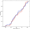Fig. 1.

Cumulative distribution of bolometric luminosity L of the FOS+HE sample (black), Pop. A (blue), and Pop. B (red).

3. Emission line profile analysis for the FOS+HE sample

3.1. Line modeling and measured parameters

In the following we consider the merit of Hβ and C IVλ1549 as VBEs. Previous work has shown that the Hβ and Mg IIλ2800 profiles are almost equally reliable estimators of the “virial” broadening in samples of moderate-to-high luminosity (e.g., Wang et al. 2009; Trakhtenbrot & Netzer 2012; Shen & Liu 2012; Marziani et al. 2013a, excluding the Mg IIλ2800 extreme Population A that is significantly broadened by a blueshifted component; Marziani et al. 2013a). However, the broad Hβ line full profile is often affected by asymmetries toward the line base and by significant line centroid shifts. Typically, the Hβ line profiles are characterized by two main asymmetries, differentially affecting sources in spectral types along the MS (Table A.1 provides the definition of spectral types):

– Pop. A: a blueshifted excess, often modeled with a blueward asymmetric Gaussian component (BLUE) related to the outflows strongly affecting the C IVλ1549 and [O III]λλ4959,5007 line profiles (e.g., Negrete et al. 2018, Paper I, and references therein).

– Pop. B: a redward asymmetry modeled with a broader redshifted (FWHM ∼ 10 000 km s⁻¹, $c (\frac{1}{2}) \sim 2000 {km s}^{- 1}$ $c\left(\frac{1}{2}\right)\sim 2000\,{\mathrm{km\,s}}^{-1}$ ) Gaussian. The very broad Gaussian is meant to represent the innermost part of the BLR, providing a simple representation of the radial stratification of the BLR in Pop. B suggested by reverberation mapping (e.g., Snedden & Gaskell 2007). This component (hereafter the very broad component, VBC) has been associated with a physical region of high-ionization virialized and closest to the continuum source (Peterson & Ferland 1986; Brotherton et al. 1994b; Sulentic et al. 2000c; Snedden & Gaskell 2007; Wang & Li 2011). While the properties of the very broad line region (VBLR) remain debatable, a decomposition of the full Hβ profile into a symmetric, unshifted Hβ component (Hβ_BC) and a Hβ_VBC provides an excellent fit to most Hβ Pop. B profiles (Sulentic et al. 2002; Zamfir et al. 2010).

Figures 4 and 5 of Paper I show the Hβ and C IVλ1549 profiles of the HE sample, and their multicomponent interpretation. To extract a symmetric, unshifted component that excludes the blueshifted excess and the VBC, we considered a model of the broad Hβ and C IVλ1549 line with the following components (see also Table A.2):

– Pop. A Hβ and C IVλ1549: an unshifted Lorentzian profile (Hβ_BC) + one or more asymmetric Gaussians to model the blueward excess (BLUE).

– Pop. B Hβ and C IVλ1549: an unshifted Gaussian (Hβ_BC) + a redshifted VBC for Hβ (Hβ_VBC). In the Hβ case, there is no evidence of a blueward excess even at the highest luminosity. However, among Pop. B sources of the HE sample, a prominent C IVλ1549 BLUE appears, implying an intensity ratio C IVλ1549/Hβ ≫ 1 in the BLUE component. The C IVλ1549 BLUE is usually fainter in the low-luminosity FOS sample Paper I.

In the fits, narrow components of both Hβ (Hβ_NC) and C IVλ1549 (C IVλ1549_NC) were included. In the case of C IVλ1549, separation of the broad and narrow component is subject to significant uncertainty, meaning that the effect of the C IVλ1549_NC needs to be carefully considered (see discussion in Sect. 3.2).

The decomposition approach summarized above has a heuristic value, as the various components are not defined on the basis of a physical model, even if the assumptions on line shapes follow from MS trends. The distinction between BC and VBC might be physically motivated (the emitting region associated with the BC is the one predominantly emitting Fe II), but the decomposition into two symmetric Gaussians is a crude approximation at best. Full profile measurements are added to avoid any exclusive dependence of the results on the profile decomposition. The full profiles of Hβ and C IVλ1549 are parameterized by the FWHM, an asymmetry index (AI), and centroid at $\frac{1}{2}$ $\frac{1}{2}$ and $\frac{1}{4}$ $\frac{1}{4}$ peak fractional intensity, $c (\frac{1}{2})$ $c\left(\frac{1}{2}\right)$ and $c (\frac{1}{4})$ $c\left(\frac{1}{4}\right)$ . The definition of centroids and AI follows Zamfir et al. (2010):

$c (\frac{i}{4}) = \frac{λ_{B} (\frac{i}{4}) + λ_{R} (\frac{i}{4})}{2 λ_{0}} c, i = 1, 2, 3; \frac{i}{4} = 0.9,$ $\begin{aligned}c\left(\frac{i}{4}\right) = \frac{\lambda _{\rm B}\left(\frac{i}{4}\right)+\lambda _{\rm R}\left(\frac{i}{4}\right)}{2 \lambda _{0}} c, \, i=1,2,3; \frac{i}{4} = 0.9, \end{aligned}$ (1)

$A . I . = \frac{λ_{B} (\frac{1}{4}) + λ_{R} (\frac{1}{4}) - 2 λ_{P}}{λ_{B} (\frac{1}{4}) + λ_{B} (\frac{1}{4})},$ $\begin{aligned}A.I. = \frac{\lambda _{\rm B}\left(\frac{1}{4}\right)+\lambda _{\rm R}\left(\frac{1}{4}\right)- 2\lambda _{\rm P}}{\lambda _{\rm B}\left(\frac{1}{4}\right)+\lambda _{\rm B}\left(\frac{1}{4}\right)}, \end{aligned}$ (2)

where λ_P is the peak wavelength, and λ_B and λ_R are the wavelengths on the blue and red side of the line at the i/4 fractional intensities. The centroids are referred to the quasar rest frame, while the AI is referred to as the peak of the line that may be shifted with respect to rest frame. A proxy to λ_P which is used in this paper is $\tilde{λ_{P}} \approx λ_{0} (1 + c (0.9) / c)$ $\tilde{\lambda_{\mathrm{P}}} \approx \lambda_{0}(1+c(0.9)/c)$ .

We assume that the symmetric and unshifted Hβ_BC and C IVλ1549_BC are the representative line components of the virialized part of the BLR. It is expedient to define a parameter ξ as follows:

$\begin{matrix} ξ_{line} = \frac{{FWHM}_{vir}}{FWHM}, \end{matrix}$ $\begin{aligned} \xi _{\mathrm{line}} = \frac{{FWHM}_{\mathrm{vir}}}{{FWHM}}, \end{aligned}$ (3)

where the FWHM_vir is the FWHM of the “virialized” component, in the following assumed to be Hβ_BC, and the FWHM is the FWHM measured on the full profile (i.e., without correction for asymmetry and shifts). The ξ parameter is a correction factor that can be defined also using components of different lines, for instance C IVλ1549 full profile FWHM and Hβ_BC, where Hβ_BC is assumed to be a reference VBE.

3.2. The C IVλ1549 narrow component in the HE sample and its role in FWHM C IVλ1549_BC estimates

In only two cases does C IVλ1549_NC contribute to the total C IVλ1549 flux of the HE Pop. B sources by more than 10%: HE2202-2557 and HE2355-4621 (Pop. B, Fig. 5 of Paper I). There is no evidence for a strong NC in the HE Pop. A sources except for HE0109-3518 where I(C IVλ1549_NC) ≲ 0.09 of the total line flux and whose C IVλ1549 profile resembles those of low-redshift sources that are less luminous by 2–3 dex (the HE0109-3518 C IVλ1549 profile is shown in Fig. 4 of Paper I).

In general, considering Hβ_BC as a reference for Pop. B sources, and comparing FWHM Hβ_BC to FWHM C IVλ1549 with and without removing the C IVλ1549_NC (i.e., to FWHM C IVλ1549_BC and FWHM C IVλ1549_BC + C IVλ1549_NC), the C IVλ1549_NC removal improves the agreement with FWHM Hβ_BC in five out of six cases when C IVλ1549_NC has an appreciable effect on the line width (in the other eight cases there is no effect because C IVλ1549_NC is too weak). The FWHMs measured on the C IVλ1549 profiles without removing the C IVλ1549_NC (i.e., FWHM C IVλ1549_BC + C IVλ1549_NC) are on average ≈−4% and −11 % of the FWHM C IVλ1549, for Pop. A and B, respectively. Therefore, (1) subtracting the C IVλ1549_NC improves the agreement between Hβ and C IVλ1549 FWHM; and (2) the average effect is too small to affect our inferences concerning the C IVλ1549 line width as a VBE in the HE sample. The C IVλ1549_NC has always been included as an independent component in the line profile fitting of Paper I, following an approach consistently applied to the low-redshift FOS sample and described by Sulentic et al. (2007).

4. Results

4.1. Hβ in the HE sample

We considered several different measurements of the Hβ width following empirical corrections derived from previous work on low-redshift samples:

– Substitution of the Hβ_BC extracted through the specfit analysis in place of the full Hβ profile.

In principle, extraction of the Hβ_BC should be the preferred approach, and the FWHM Hβ_BC the preferred VBE. To test the reliability of the FWHM values, we performed Monte-Carlo repetitions of the Hβ fit for Pop. B sources with the broadest lines (FWHM Hβ_BC ∼ 7000 km s⁻¹, and FWHM Hβ_VBC ∼ 11 000 km s⁻¹), assuming an S/N ≈ 20¹, weak and relatively broad [O III]λλ4959,5007, a changing noise pattern, and initial values of the fitting. The values of FWHM Hβ_BC and Hβ_VBC were chosen to represent the broadest lines, where FWHM Hβ_BC measurements might be affected by a degeneracy in the BC+VBC decomposition. The dispersion of the Monte Carlo FWHM distribution is almost symmetric, and implies typical FWHM Hβ_BC uncertainties ≈10% at 1σ confidence level. Therefore, the blending should not be a source of strong bias or of large uncertainties in the Hβ_BC and Hβ_VBC FWHM². However, we still expect that in the case of very broad profiles, and low S/N or low dispersion, the decomposition of the Hβ profile into Hβ_BC and Hβ_VBC is subject to large uncertainties that are difficult to quantify. To retrieve information on the Hβ_BC we introduce several corrections that can be applied to the full Hβ profile without any multicomponent fitting (which also renders the results model-dependent).

– Symmetrization of the full profile: $F W H M_{symm} = F W H M - - 2 c (\frac{1}{2})$ $FWHM_{\mathrm{symm}} = FWHM -- 2c\left(\frac{1}{2}\right)$ (symm in Fig. 2). The physical explanation behind the symmetrization approach involves an excess radial velocity on the red side that may be due to gas with a radial infall velocity component, with velocity increasing toward the central black hole (e.g., Wang et al. 2017, and references therein). Generally speaking, redward displacements of line profiles have been explained by invoking a radial infall component plus obscuration (Hu et al. 2008; Ferland et al. 2009);

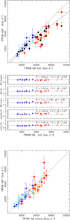Fig. 2.

Virial broadening estimators based on Hβ, with several corrections applied to the HE sample. Top square panel: FWHM Hβ_BC (blue (Pop. A) and red (Pop. B)) with error bars, symmetrized FWHM Hβ (symm, black), and FWHM Hβ corrected according to spectral type (st, aquamarine and dark orange for Pop. A and B respectively) versus FWHM of the full Hβ profile. The gray line traces the correction (corr) following the relation of Sulentic et al. (2006a) reported in Sect. 4. Middle panels: ratios of FWHM after various corrections vs. full profile FWHM. Panels from top show: BC/symm, BC/st, BC/corr, symm/ st, corr/st. Average values, standard deviation and normalized $χ_{ν}^{2}$ $\chi^{2}_{\nu}$ are reported in the upper-right corner of the panels. Bottom square panel: BC, spectral type st and reverberation corrected (corr, open symbols) FWHM values vs. symmetrized FWHM.

– Substitution of the FWHM Hβ_BC with the FWHM measured on the full broad profile of Hβ, corrected according to its spectral type. The spectral types have been assigned following Sulentic et al. (2002, for a conceptually equivalent approach see Shen & Ho 2014). The corrections are as defined from the analysis of the Hβ profile in a large SDSS-based sample at 0.4 ≲ z ≲ 0.7 (labeled as st in Fig. 2). In practice, this means to correct Hβ for Pop. B sources by a factor ξ_Hβ ≈ 0.8 (Marziani et al. 2013b) and extreme population A sources (R_FeII ≥1) by a factor ξ_Hβ ≈ 0.9. On average, spectral types A1 and A2 show symmetric profiles for which ξ_Hβ ≈ 1. Recent work confirmed that the effect of a blueshifted excess on the full profile of Hβ is small at half-maximum, 0.9 ≲ ξ_Hβ ≲ 1.0 (Negrete et al. 2018). We assume ξ_Hβ = 0.9 as an average correction for ST A3 and A4. The ratio we derive between BC and full profile FWHM of HE Pop. B Hβ is ≈0.82 ± 0.09, consistent with the same ratio estimates at moderate luminosity (Marziani et al. 2013b). The st correction can be summarized as follows:

ST	ξHβ

A3 – A4	0.9
A1 – A4	1.0
B1 – B1 +	0.8

– Correction of the width of the full broad Hβ profile based on the one derived at low z by pairing the observed full broad Hβ FWHM to the best width estimator from reverberation mapping, following the relation FWHM_c ≈ 1.14 FWHM–601 – 0.0000217FWHM² derived by Sulentic et al. (2006a, labeled corr);

Figure 2 shows that these corrections all provide similar results if applied to the HE sample FWHM Hβ. Error bars of Fig. 2 were estimated propagating the uncertainty values reported in Paper I for the full profiles, and those derived from specfit for the line components (assuming a minimum error of 10%).

The middle panels of Fig. 2 show the ratios of corrected FWHM measurements as a function of the FWHM of the full Hβ profile. The low $χ_{ν}^{2}$ $\chi^{2}_{\nu}$ indicates that the $χ_{ν}^{2}$ $\chi_{\nu}^{2}$ associated with the ratios between BC and symm, and BC and st is not significantly different from unity. In the case of BC and corr the two measurements are different but only at 1σ confidence level. The F tests do not exclude that BC, symmetrization, st, and reverberation corrections can be equivalent at a confidence level of 2σ. The bottom panel of Fig. 2 shows the behavior of the full and corrected FWHM versus the “symmetrized” Hβ FWHM. We consider the symmetrization, as it is relatively easy to apply (once the quasar rest frame is known), and the st correction (that does not even require the knowledge of the rest frame) as reference corrections. We reiterate the fact that these corrections are relatively minor but still significant: a 20% correction translates into a factor 1.44 correction in M_BH. They do not undermine the value of the full line width of Hβ as a useful VBE (with the caveats discussed in Sect. 5.2), since the Hβ full line width remains preferable to the uncorrected C IVλ1549 width for most objects.

4.2. C IVλ1549 in the full HE+FOS sample

The results on the HE C IVλ1549 profiles do not bode well for the use of C IVλ1549 FWHM as a VBE, as also found by Sulentic et al. (2007) and other workers (Sect. 5.1 for a brief critical review). The presence of very large blueshifts in both Pop. A and B makes the situation even more critical than at low L. Figure 3 (top panel) shows that there is no obvious relation between the FWHM of C IVλ1549 and the FWHM of Hβ if FOS+HE data are considered together.

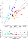Fig. 3.

Top panel: FWHM(C IVλ1549) vs. FWHM(Hβ) (full profiles) for the FOS+HE sample. Data points are color-coded according to sample and population: HE Pop. A – blue circles (), HE Pop. B – red squares (), FOS Pop. A – aquamarine circles (), and FOS Pop. B – golden squares (). Best fitting least-square lines (dashed) are shown in blue for all Pop. A and red for all Pop. B. The black dot-dashed line is the equality line. The continuous gray line is the expected FWHM following the correction of Sulentic et al. (2006a, corr). Lower panel: ratio between FWHM C IVλ1549 and FWHM Hβ as a function of FWHM (Hβ).

For the Pop. A sources in the HE+FOS sample, C IVλ1549 is broader than Hβ, apart from in two cases in the HE sample, and FWHM(C IVλ1549) shows a broad range of values for similar FWHM Hβ, that is, FWHM(C IVλ1549) is almost degenerate with respect to Hβ. The C IVλ1549 line FWHM values are so much larger than the ones of Hβ, thus making it possible that the M_BH derived from FWHM C IVλ1549 might be higher by even more than one order of magnitude. Formally, the Pearson’s correlation coefficient r ≈ 0.52 is highly significant for a sample of n = 43, with significance at a confidence level ≈4.5σ. A weighted least-square fit yields FWHM(C IVλ1549) = (1.822 ± 0.204)FWHM(Hβ) + (−624 ± 677) km s⁻¹, with a significant scatter, rms ≈ 1959 km s⁻¹. Unfortunately it is not possible to apply a simple C IVλ1549 symmetrization as done for Hβ: subtracting $2 \cdot c (\frac{1}{2})$ $2 \cdot c\left(\frac{1}{2}\right)$ from FWHM C IVλ1549 leads to corrections that are unrealistically large.

If we combine the Pop. B FOS and HE samples, FWHM C IVλ1549 and Hβ become loosely correlated (the Pearson’s correlation coefficient is ≈0.4, significant at P ≈ 98% for a sample of 33 objects). A weighted least-square fit yields FWHM(C IVλ1549) ≈ (0.764 ± 0.165)FWHM(Hβ) + (810 ± 1030) km s⁻¹, and rms ≈ 1090 km s⁻¹, with a significant deviation from the 1:1 relation. In the case of Pop. B sources, the trend implies FWHM C IVλ1549 ∼ FWHM Hβ, and even a slightly narrower FWHM C IVλ1549 with respect to Hβ.

The large scatter induced by using an uncorrected C IVλ1549 line FWHM may have contributed to the conclusion that line width does not contribute significantly to M_BH determinations (Croom 2011).

4.3. Practical usability of C IVλ1549_BC

The fitting procedure scaled the Hβ profile to model the red side of C IVλ1549 meaning that the FWHM C IVλ1549_BC estimate is not independent from FWHM Hβ_BC. The FWHM values of the two BCs are in agreement because of this enforced condition.

The C IVλ1549_BC extraction is very sensitive to the assumed rest frame, and also requires that the C IVλ1549 line be cleaned from contaminants such as Fe II (weak) and He IIλ1640 (moderate, but flat-topped and gently merging with the C IVλ1549 red wing; Marziani et al. 2010; Fine et al. 2010; Sun et al. 2018). Without performing a line profile decomposition, one can consider the width of the red side with respect to rest frame as the half width at half maximum (HWHM) of the virial component. Again this requires (1) an accurate redshift that can be set, in the context of high-redshift quasars, either by using the Hβ narrow component or by the [O II]λ3727 doublet (Eracleous & Halpern 2004; Hu et al. 2008), and (2) the decomposition from He IIλ1640 emission blended on the C IVλ1549 red side. If [O II]λ3727 is covered, then Mg IIλ2800 is also likely to be covered. As mentioned in Sect. 3, the Mg IIλ2800 line width is a reliable VBE for the vast majority of type-1 AGNs. The same is not true for C IVλ1549. For spectra where C IVλ1549 is conveniently placed at z ≳ 1.45, the [O II]λ3727 line is shifted beyond 9000 Å, a domain where intense sky emission makes it difficult to analyze a relatively faint narrow line. The extraction of C IVλ1549_BC is therefore not a viable solution if single-epoch C IVλ1549 observations are available without the support of at least a narrow LIL that may set a reliable rest frame. This is unlikely to occur on the same optical spectra. An alternative strategy for M_BH estimation using C IVλ1549 FWHM should consider the origin of the C IVλ1549 nonvirial broadening.

4.4. Reducing C IVλ1549 to a VBE estimator consistent with Hβ

The main results of Paper I suggest a strong dependence of the C IVλ1549 blueshift on L/L_Edd, especially above a threshold value L/L_Edd ≈ 0.2 ± 0.1 (Sulentic et al. 2014, and references therein). A correlation between Eddington ratio and the FWHM(C IVλ1549) to FWHM(Hβ) ratio (i.e., 1/ξ_CIV, cf., Saito et al. 2016) is detected at a high significance level (Pearson’s correlation coefficient r ≈ 0.55) joining all FOS RQ sources of Sulentic et al. (2007; Fig. 4). In this context, L/L_Edd was computed from the M_BH scaling law of Vestergaard & Peterson (2006) using the FWHM of Hβ and λL_λ(5100). A bisector best fit with SLOPES (Feigelson & Babu 1992) yields

$\begin{matrix} log \frac{1}{ξ_{CIV}} \approx (0.426 \pm 0.043) \frac{L}{L_{Edd}} + (0.401 \pm 0.035) . \end{matrix}$ $\begin{aligned} \log \frac{1}{\xi _\mathrm{CIV} } \approx (0.426 \pm 0.043) \frac{L}{L_\mathrm{Edd} } + (0.401 \pm 0.035). \end{aligned}$ (4)

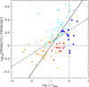Fig. 4.

Relation between the logarithm of the FWHM ratio of C IVλ1549 to Hβ and the logarithm of the Eddington ratio L/L_Edd. The vertical dot-dashed line traces the Eddington limit. The colors and shapes of symbols are as in Fig. 3. The dashed line is an unweighted least-squares fit, and the filled line was obtained with the bisector method (Feigelson & Babu 1992).

An L/L_Edd-dependent correction is in principle a valid approach. However, how to calculate L/L_Edd from UV spectra without resorting to Hβ observations is not obvious. In addition, FWHM Hβ is strongly affected by orientation and yields biased values of L/L_Edd (Sect. 5.2.2). Both FWHM(Hβ_BC)/FWHM(C IVλ1549) and $c (\frac{1}{2})$ $c\left(\frac{1}{2}\right)$ are correlated with Eddington ratio. Consistently, the C IVλ1549 blueshift is correlated with FWHM C IVλ1549 (Paper I, Coatman et al. 2016), and accounts for the broadening excess in the C IVλ1549 FWHM. Measurements of the C IVλ1549 blueshift or the FWHM(Hβ_BC)/FWHM(C IVλ1549) can be used as proxies for L/L_Edd. At the same time, Paper I reveals a weaker correlation with L, which is expected in the case of a radiation-driven wind. If the correction factor is ξ_CIV = FWHM(Hβ_BC)/FWHM(C IVλ1549), then it should include a term in the form 1/ζ(L, L/L_Edd).

4.5. Calibrating empirical corrections on FWHM C IVλ1549

Coatman et al. (2017) introduced a nonparametric measurement of the C IVλ1549 blueshift associated with the wavelength that splits the line flux in equal parts on its blue and red sides (flux bisector). The flux bisector is strongly correlated with $c (\frac{1}{2})$ $c\left(\frac{1}{2}\right)$ and $c (\frac{1}{4})$ $c\left(\frac{1}{4}\right)$ , and $c (\frac{1}{2})$ $c\left(\frac{1}{2}\right)$ and $c (\frac{1}{4})$ $c\left(\frac{1}{4}\right)$ are correlated among themselves in the FOS+HE sample (Pearson’s r ≈ 0.95): $c (\frac{1}{2}) = (0.773 \pm 0.307) c (\frac{1}{4}) - (58 \pm 65) km s^{- 1}$ $c\left(\frac{1}{2}\right) = (0.773 \pm 0.307) c\left(\frac{1}{4}\right) -(58 \pm 65)\,\mathrm{km \, s^{-1}}$ . The bisector correlation is stronger with $c (\frac{1}{4})$ $c\left(\frac{1}{4}\right)$ (Pearson’s correlation coefficient r ≈ 0.98), with flux bisector $\sim (0.98 \pm 0.04) c (\frac{1}{4}) + (220 \pm 110) km s^{- 1}$ ${\sim}(0.98 \pm 0.04) c\left(\frac{1}{4}\right) +(220 \pm 110)\, \mathrm{km \, s^{-1}}$ (Fig. 5). The lower panel of Fig. 5 shows a few objects where the difference between the $c (\frac{1}{4})$ $c\left(\frac{1}{4}\right)$ and the flux bisector is ≳20%; these sources are either with small shifts (within the measurement uncertainties; shaded area of Fig. 5), or sources strongly affected by broad absorptions, for which measurement of blueshift is tricky regardless of the method employed. Therefore, it is possible to apply Eq. (4) of Coatman et al. (2017) substituting the $c (\frac{1}{4})$ $c\left(\frac{1}{4}\right)$ to the flux-bisector blueshift measurements:

$\begin{matrix} ξ_{CIV, 0} = \frac{1}{a (- \frac{c (\frac{1}{4})}{1000}) + b}, \end{matrix}$ $\begin{aligned} \xi _\mathrm{CIV,0} = \frac{1}{a \left(- \frac{c\left(\frac{1}{4}\right)}{1000} \right) + b} , \end{aligned}$ (5)

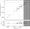Fig. 5.

Top panel: bisector flux estimator of Coatman et al. (2017) vs. $c (\frac{1}{4})$ $c\left(\frac{1}{4}\right)$ , in km s⁻¹. The dot-dashed line is the equality line. Bottom panel: percentage residuals. The shaded areas indicate the average errors of measurements at a 2σ confidence level computed from Table 4 of Paper I.

with a = 0.41 ± 0.02 and b ≈ 0.62 ± 0.04 (the minus sign is because Coatman et al. (2017) assumed blueshifts to be positive), to correct the FWHM C IVλ1549 of the FOS+HE sample. The resulting trend is shown in Fig. 6. Equation (4) of Coatman et al. (2017) undercorrects both Pop. A and B sources at low L (the FOS sample) and provides a slight overcorrection for the HE sources. The correction of Coatman et al. (2017) does not yield FWHM (C IVλ1549) in agreement with the observed values of FWHM(Hβ). This does not necessarily mean that the FWHM(C IVλ1549) values are incorrect, as FWHM(Hβ) is likely more strongly affected by orientation effects than FWHM(C IVλ1549); see the discussion in Sect. 5.2.

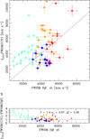Fig. 6.

Top panel: FWHM(C IVλ1549) C16 (i.e., corrected following Coatman et al. 2016), vs. FWHM(Hβ) st for the FOS+HE sample. Meaning of symbols is the same as for Fig. 3. The black dot-dashed line is the equality line. Bottom panel: residuals. Average ratio, dispersion, and $χ_{ν}^{2}$ $\chi^{2}_{\nu}$ refer to all sources.

A correction dependent on luminosity reduces the systematic differences between the various samples in the present work but it has to be separately defined for Pop. A and B (Fig. 7). The following expression provides a suitable fitting law, with a, b, c different for Pop. A and B.

$\begin{matrix} ξ_{CIV, 1} = \frac{1}{b (a - log λ L_{λ} (1450)) \cdot (| \frac{c (\frac{1}{2})}{1000} |) + c} \cdot \end{matrix}$ $\begin{aligned} \xi _\mathrm{CIV,1} = \frac{1}{b \left(a - \log \lambda L_{\lambda }(1450)\right) \cdot \left(\big |\frac{c\left(\frac{1}{2}\right)}{1000}\big |\right) + c} \cdot \end{aligned}$ (6)

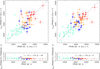Fig. 7.

Top left panel: ξ_CIVFWHM(C IVλ1549) i.e., FWHM(C IVλ1549) after correction for blueshift and luminosity dependence following Eq. (6) vs. FWHM(Hβ) cm for the FOS+HE sample. The black dot-dashed line is the equality line, and the meaning of the color-coding is the same as in Fig. 3. Top right: as in top panel but with ξ_CIV computed from Eq. (7).

Here we consider the $c (\frac{1}{2})$ $c\left(\frac{1}{2}\right)$ because of its immediate connection with the FWHM, and because it is highly correlated with $c (\frac{1}{4})$ $c\left(\frac{1}{4}\right)$ (Sect. 5.5). Equation (6) is empirical: it entails a term proportional to shift and one to the product of log L₁₄₅₀ and shift. Multivariate, nonlinear lsq results for Eq. (6) are reported in the first rows of Table 1. For Pop. A, the correction is rather similar to the one of Coatman et al. (2017), and is driven by the large blueshifts observed at high L/L_Edd. The luminosity-dependent factor accounts for low-luminosity sources that are not present in the Coatman et al. (2017) sample. The use of the absolute value operator provides an improvement with respect to the case in which blueshifts are left negative. There are only three objects for which $c (\frac{1}{2})$ $c\left(\frac{1}{2}\right)$ is positive. The improvement is understandable if one considers any C IVλ1549 shift as affecting the difference between the FWHM of C IVλ1549 and Hβ. An A(+) sample was defined from the Pop. A sample minus three objects with positive $c (\frac{1}{2})$ $c\left(\frac{1}{2}\right)$ , that is, all A(+) sample sources show blueshifts. No significant improvement was found with respect to the previous sample.

Table 1.

Fits of ξ_CIV.

The correction for Pop. B is less well defined, considering the uncertainty in a, and the low value of b (Table 1). The corrections for Pop. B still offer an improvement because they remove significant bias (as evident by comparing Figs. 3 and 7). In practice, for Pop. B, at low L the ξ_CIV could be considered constant to a zero-order approximation, with ξ_CIV ∼ 1. In other words, when the velocity field is predominantly virial, and no prominent blueshifted component affects the line width, C IVλ1549 may be somewhat broader than Hβ as expected for the stratification revealed by reverberation mapping of lines from different ionic species (Peterson & Wandel 1999, 2000). The fit is consistent with ξ_CIV depending on shift but only weakly on luminosity. The Pop. B correction is so ill-defined that larger samples are needed for a better determination of its coefficients.

Slightly different fitting laws

$\begin{matrix} ξ_{CIV, 2} = \frac{1}{a + b log λ L_{λ} (1450) + c \frac{c (\frac{1}{2})}{1000}}, \end{matrix}$ $\begin{aligned} \xi _\mathrm{CIV,2} = \frac{1}{a + b \log \lambda L_{\lambda }(1450) + c \frac{c\left(\frac{1}{2}\right)}{1000}} , \end{aligned}$ (7)

which considers a linear combination log λL_λ(1450) and shift, and

$\begin{matrix} ξ_{CIV, 3} = \frac{1}{a - b log λ L_{λ} (1450) \cdot \frac{c (\frac{1}{2})}{1000}}, \end{matrix}$ $\begin{aligned} \xi _\mathrm{CIV,3} = \frac{1}{a - b \log \lambda L_{\lambda }(1450) \cdot \frac{c\left(\frac{1}{2}\right)}{1000}} , \end{aligned}$ (8)

which assumes a dependence from the product log λL_λ(1450) and shift, provide consistent results, with fitting parameters, 1σ confidence level associated uncertainty, and root mean square (rms) residuals of ξ_CIV reported in Table 1. The fitting relations yield a lower residual scatter in ξ_CIV than assuming no luminosity dependence. For instance, using Eq. (7) we obtain a scatter in ξ_CIV, 2 that is a factor 1.86 lower than if Eq. (5) is used. We also considered the AI in place of $c (\frac{1}{2})$ $c\left(\frac{1}{2}\right)$ in Eq. (6) (without the absolute value operator; bottom rows of Table 1). The AI has a non-negligible advantage to be independent from the choice of the rest frame. The AI is correlated with both $c (\frac{1}{4})$ $c\left(\frac{1}{4}\right)$ and $c (\frac{1}{2})$ $c\left(\frac{1}{2}\right)$ , and shows higher correlation with $c (\frac{1}{4})$ $c\left(\frac{1}{4}\right)$ (Pearson’s r ≈ 0.66). However, the scatter in ξ_CIV, A.I. is unfortunately large, and would imply a scatter ≈1.5 higher in M_BH estimates than in the case where Eq. (6) is considered for Pop. A.

If Pop. A and B are considered together, the final scatter in ξ_CIV is close for the different fitting function (Eq. (6) yields a slightly better result) but much higher than if Pop. A and B are kept separated. It is therefore necessary to distinguish between Pop. A and B as the intrinsic structure of their BLR may be different (e.g., Goad & Korista 2014; Wang et al. 2014a). In Pop. B, at low L/L_Edd, the lines are mainly broadened following a virial velocity field (Peterson & Wandel 2000). The relative prominence of the blueshifted to the virialized component (ratio BLUE over BC) is lower in Pop. B than in Pop. A, a consequence of the low L/L_Edd for Pop. B sources. Both properties are expected to contribute to the overall consistency between Hβ and C IVλ1549 profiles in Pop. B sources. At any rate, ξ_CIV should always be ≲1, with ξ_CIV ≈ 1 for Pop. B at low L, and ξ_CIV ≪ 1 in case of very large shifts, as in Pop. A at high L.

It is possible in most cases to distinguish between Pop. A and B from the UV spectrum emission blend, making the correction applicable at least to a fraction of all quasars in large samples. Several criteria were laid out by Negrete et al. (2014): (1) broad line width; (2) evidence of a prominent red wing indicative of a VBC; and (3) prominence of C III]λ1909. Population B sources show a C IVλ1549 red wing and strong C III]λ1909 in the 1900 Å. Extreme Pop. A (xA) sources are easy to recognize; they show strong Al IIIλ1860 in 1900 Å blend and low W(C IVλ1549). A prototypical composite spectrum of xA sources is shown by Martínez-Aldama et al. (2018). However, some intermediate cases along the MS (i.e., spectral type A1) may be easier to misclassify. Also, with only the UV spectral range available, the redshift estimate may be subject to large errors. Negrete et al. (2014) provide a helpful recipe; however, their recipe applied to three of their eight sources allowed for a precision of ∼100 km s⁻¹ in the rest frame, but the remaining five had an average uncertainty ≳500 km s⁻¹.

5. Discussion

Recently, the problems outlined in earlier works by Sulentic et al. (2007) and Netzer et al. (2007) have been ascribed to a “bias” in the C IVλ1549 M_BH estimates (Denney et al. 2016). The C IVλ1549 M_BH bias is dependent on the location in the 4DE1 quasar MS: Figs. 2 and 3 clearly show the different behavior for Populations A and B. By the same token, an L/L_Edd-dependent correction is in principle a valid approach, as L/L_Edd is probably one of the main drivers of the MS (Boroson & Green 1992; Sulentic et al. 2000a; Sun & Shen 2015). Unfortunately, several recent works still ignore 4DE1-related effects (or, in other words, MS trends). For instance, scaling laws derived from the pairing of the virial products for all sources with reverberation mapping data should be viewed with care (as shown by the reverberation mapping results of Du et al. 2018).

5.1. C IVλ1549 and Hβ as M_BH estimators: input from recent works

Attempts at using the C IVλ1549 as a VBE have been renewed in the last few years, not least because C IVλ1549 can be observed in the optical and NIR spectral ranges over which high-redshift quasars have been discovered and are expected to be discovered in the near future. The large C IVλ1549 blueshifts indicate that part of the BLR gas is under dynamical conditions that are far from virialized equilibrium. At high Eddington ratios, ionized gas may escape from the galactic bulge, and even be dispersed into the intergalactic medium, as predicted by numerical simulations (e.g., Debuhr et al. 2012), and at high luminosity (log L ≳ 47 [erg s⁻¹]) they might have a significant feedback effect on the host galaxy (Marziani et al. 2016).

A firm premise is that the disagreement between Hβ and C IVλ1549 mass estimates is not a matter of S/N (Denney et al. 2013). The C IVλ1549 line width suffers from systematic effects which emerge more dramatically at high S/N, i.e., when it is possible to appreciate the complexity of the C IVλ1549 profile. Given this basic result, recent literature can be tentatively grouped into three main strands: (1) low-redshift studies involving FOS and Cosmic Origin Spectrograph (COS) spectra to cover C IVλ1549; (2) high-redshift studies, where the prevalence of large C IVλ1549 shifts is high; and (3) studies attempting to correct the C IVλ1549 FWHM and reduce it to an equivalent of Hβ, some of them employing results that are directly connected to the MS contextualization of quasar properties.

Low-redshift studies. A large systematic analysis of the C IVλ1549 profiles paired to Hβ emission was carried out using HST/FOS (in part used for the present work) and optical observations (Sulentic et al. 2007). The results of this study emphasized the role of the C IVλ1549 line width in the M_BH estimates. Figure 6 of Sulentic et al. (2007) clearly shows the importance of placing sources in an E1 context: estimates of the masses could be easily overestimated by a factor ≲100 for extreme Pop. A sources such as I Zw 1, while for Pop. B, C IVλ1549 and HβM_BH estimates appeared more consistent albeit with a large scatter. The line width (be it the FWHM or the velocity dispersion σ) remains a major factor in C IVλ1549 versus HβM_BH determinations since broadening enters squared in the scaling laws (Kelly & Bechtold 2007). Similar warnings on using C IVλ1549 FWHM were issued by Netzer et al. (2007). Low-redshift samples are less affected by the Eddington ratio bias that is cutting low-Eddington ratio sources at a given M_BH for a fixed flux limit (Sulentic et al. 2014). Therefore, it may not be surprising to find studies based on excellent spectra that find an overall consistency between Hβ and C IVλ1549 M_BH estimates. Intrinsic scatter is probably high if full line widths without corrections are used: Tilton & Shull (2013) find ≈0.5 dex from COS observations of low-redshift quasars. Denney et al. (2013) claim to be able to reduce the disagreement between M_BH derived using Hβ and C IVλ1549 to ≈0.24 dex by using the velocity dispersion of the C IVλ1549 line. Since the C IVλ1549 profile in the Denney et al. (2013) sample almost never shows large blueshifts, which may be associated to a velocity shear in outflowing gas, these results appear consistent with the Pop. B properties of the FOS sample.

High-redshift studies. These studies generally agree on the fact that the C IVλ1549 FWHM is poorly correlated with the Balmer line FWHM. Shen & Liu (2012) describe the scatter between C IVλ1549 and Hβ FWHM as due to an irreducible part (≈0.12 dex), and a part that correlates with the blueshift of the C IVλ1549 centroid relative to that of Hβ. These latter authors propose scaling laws in which the virial assumption is abandoned, that is, with the exponent of the line FWHM being significantly different from two. For C IVλ1549, this means correcting for the overbroadening associated with the nonvirial component. The scaling law introduced by Park et al. (2013) is consistent with the approach by Shen & Liu (2012) and implies M_BH ∝ FWHM^0.5, that is, a FWHM dependence that is very different from the one expected from a virial law (M_BH ∝ FWHM²). As shown in Fig. 8, the scaling law suggested by Park et al. (2013) applied to the HE sample properly corrects for the overbroadening of Pop. A sources, but overcorrects the width of Pop. B, yielding a large deviation from the Hβ-derived M_BH values (on average ≈0.28 dex).

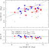Fig. 8.

Black hole mass computed from the fiducial relation of Vestergaard & Peterson (2006) based on FWHM Hβ vs. the ones computed from the C IVλ1549 FWHM following Park et al. (2013), for Pop. A (blue) and B (red) HE sources. Values of M_BH obtained from the Vestergaard & Peterson (2006) C IVλ1549 scaling law after the correction suggested by Brotherton et al. (2015, small dots) are shown by small open circles. Lower panel: residuals as a function of M_BH. The average and the scatter reported for Populations A and B refer to the Park et al. (2013) scaling laws.

Studies exploiting MS trends. The results reported in Sect. 4 and in Paper I indicate that any solution seeking to bring C IVλ1549 M_BH estimates into agreement with the ones from Hβ cannot exclude the strong L/L_Edd dependence of the C IVλ1549 blueshift that is in turn affecting the C IVλ1549 FWHM (Fig. 4). The discussion in Sects. 3 and 4.5 here identifies the C IVλ1549 blueshift as an expedient L/L_Edd proxy. Any parameterization of the blueshifted amplitude such as $c (\frac{1}{2})$ $c\left(\frac{1}{2}\right)$ , the flux bisector of Coatman et al. (2016), or the ratio FWHM(C IVλ1549)/FWHM(Hβ) takes into account the MS trends in C IVλ1549 properties due to the L/L_Edd and C IVλ1549 blueshift correlation. Another L/L_Edd proxy may involve the Si IVλ1397/C IVλ1549 peak ratio: at low Si IVλ1397/C IVλ1549 the M_BH is underestimated with respect to Hβ, and at high Si IVλ1397/C IVλ1549 the mass is overestimated (Brotherton et al. 2015). Since the ratio Si IVλ1397/C IVλ1549 is a known 4DE1 correlate (Wills et al. 1993; Bachev et al. 2004), these results confirm that FWHM C IVλ1549 leads to an overestimate of M_BH for Pop. A (as Pop. A outflows produce blueshifted emission that significantly broadens the line (Fig. 3; cf. Denney et al. 2012). In our sample, however, applying the correction suggested by Brotherton et al. (2015), that is, $δ log M \approx - 1.23 log \frac{1400}{CIV} - 0.91,$ $\delta \log M \approx - 1.23 \log \frac{1400}{\mathrm{CIV}} - 0.91,$ to the masses derived from the Park et al. (2013) would move the M_BH of Pop. B further down, leading to a further increase of the overcorrection, and also destroying the agreement for Pop. A sources; on top of the ∝FWHM^0.5 law, the additional correction is δlog M ≈ −0.91 if $\frac{1400}{CIV} \sim 1$ $\frac{1400}{\mathrm{CIV}} \sim 1$ . The correction is lower but still negative for most Pop. B sources where $\frac{1400}{CIV} \sim 0.3$ $\frac{1400}{\mathrm{CIV}} \sim 0.3$ , exacerbating the disagreement between the Hβ and C IVλ1549 derived masses. Better consistency is achieved if the correction of Brotherton et al. (2015) is applied to the Vestergaard & Peterson (2006) scaling law for C IVλ1549. In this case (shown in Fig. 8 by small open circles) the correction for Pop. A still implies non-negligible systematic residuals δlog M = log M_BH(Hβ_BC) – log M_BH(C IVλ1549) ≈0.23. The average residual is higher for Pop. B M_BH, with δlog M ≈ 0.27, and scatter ≈0.39 dex.

Assef et al. (2011) used a sample of approximately ten sources with optical spectra covering C IVλ1549 and NIR spectra covering Hβ or Hα and showed that M_BH estimates can be made consistently. The approach of Assef et al. (2011) may also be understood as a correction related to the MS. Assef et al. (2011) suggest that much of the dispersion in their virial mass is caused by the poor correlation between λL_λ at 5100 Å and at 1350 Å rather than between their line widths. Their Figs. 14 and 15 show that the FWHM C IVλ1549 to Hβ ratio depends on the flux ratio at 1350 Å and 5100 Å, which is an MS correlate (Laor et al. 1997; Shang et al. 2011). The Assef et al. 2011 sample of gravitationally lensed quasars might have lowered the Eddington ratio bias described by Sulentic et al. (2014), leading to a preferential section of Pop. B quasars, and better agreement between Hβ and C IVλ1549 line width.

5.2. A virialized component

5.2.1. Similar Hβ and C IVλ1549 luminosity trends

A systematic increase in line width in the HE sample is expected if the line broadening is predominantly virial: Fig. 5 of Paper I shows that there are no FWHM Hβ ≲ 3000 km s⁻¹ at log L ≳ 47 [erg s⁻¹]. Figure 9 here shows that a similar increase in FWHM as a function of luminosity is occurring in the FOS+HE sample for both Hβ and C IVλ1549. The FWHM ratio between C IVλ1549 and Hβ does not instead appear strongly influenced by L, leading to the interpretation that the broadening of both lines – even if the C IVλ1549 centroid measurements are significantly affected by an outflowing component – may be mostly related to the gravitational effects of the supermassive black hole (as further discussed below). As mentioned, Balmer lines provide a VBE up z ≳ 2, and the results of Paper I extended this finding to the highest luminosities. For C IVλ1549, Fig. 9 and the correlation $F W H M - c (\frac{1}{2})$ $FWHM-c\left(\frac{1}{2}\right)$ justify the assumption of a virial broadening component coexisting with a nonvirial one (Wang et al. 2011).

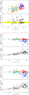Fig. 9.

Hβ and C IVλ1549 profile parameter comparison as a function of luminosity. Top panels: behavior of FWHM C IVλ1549 and Hβ (upper half) and of the ratio FWHM(C IVλ1549)/FWHM(Hβ) as a function of L (lower half), for FOS (golden and pale blue) and HE sample (red and blue). The yellow band identifies the region where FWHM(C IVλ1549)/FWHM(Hβ) = 1 within the errors. Middle panels: $c (\frac{1}{2})$ $c\left(\frac{1}{2}\right)$ of Hβ and C IVλ1549 (upper half), and difference $δ (\frac{1}{2})$ $\delta\left(\frac{1}{2}\right)$ as a function of L (lower half). Square symbols indicate Pop. B, circles Pop. A. Lines trace an unweighted least-squares fit for the Pop. A (black) and for Pop. B (red) sources. Bottom panels: as in top panels but for $c (\frac{1}{4})$ $c\left(\frac{1}{4}\right)$ and $δ (\frac{1}{4})$ $\delta\left(\frac{1}{4}\right)$ . The vertical dotted lines join Hβ and C IVλ1549 parameters for the same object (e.g., they are not error bars).

5.2.2. Orientation effects on Hβ

A large part of the C IVλ1549 – Hβ scatter is expected to be due to orientation effects. The issue of orientation effects remains open for RQ sources, and orientation effects are most likely strongly affecting the FWHM of Hβ (Mejía-Restrepo et al. 2018b), even if it remains hard to distinguish them from other physical factors (such as M_BH and L/L_Edd). A clue is given by the 4DE1 predictions at extreme orientations: objects observed near the disk rotation axis (i.e., nearly pole-on) have the smallest FWHM Hβ, the strongest Fe II and Ca II intensities (Dultzin-Hacyan et al. 1999), the largest soft X excess, and the largest C IVλ1549 blue shifts/asymmetries. These predictions are motivated by the physical scenarios involving an accretion disk–wind system. From a pole-on orientation we should see the smallest Doppler broadening of virially dominated Hβ-emitting clouds, and the strongest intensity of Fe II and other LILs if they are emitted from clouds in the outer part of the disk (Martínez-Aldama et al. 2015). We should also observe the largest contribution of the soft X excess if it is related to disk emission (Wang et al. 1996, 2014b; Boller et al. 1996). Finally, if a wind is associated with an optically thick disk, and its dynamics is dominated by radiation pressure, HILs such as C IVλ1549 emitted in the wind would show the largest blueshifts (if the receding part of the flow is shielded from view). The case of I Zw 1 provided a prototypical case in which a flattened LIL-emitting systems and a radial outflow could be seen at small inclination (e.g., Marziani et al. 1996; Leighly 2004).

From a more modern perspective, there are several indications that the low-ionization BLR is a flattened system (Mejía-Restrepo et al. 2017, 2018a; Negrete et al. 2017, 2018). We see the clearest evidence at the MS extrema: extreme Pop. B sources radiating at very low L/L_Edd frequently show LIL profiles consistent with geometrically thin accretion disk profiles (e.g., Chen & Halpern 1989; Strateva et al. 2003; Storchi-Bergmann et al. 2017), which may be hidden in the majority of Pop. B sources (Bon et al. 2007, 2009). A highly flattened LIL-BLR is also suggested in blazars, which are also Pop. B low-radiatiors (Decarli et al. 2011), by comparing the virial product to mass estimates obtained from the correlation between M_BH and the host galaxy luminosity. At the other end of the MS, extreme Pop. A quasars show deviations from virial luminosity estimates consistent with the effect of orientation on the line width, if the emitting region is highly flattened (Negrete et al. 2018). A flattened low-ionization BLR is also suggested by comparing the virial product to mass estimates obtained from accretion disk fits to the SED (Mejía-Restrepo et al. 2017, 2018a).

The effect of orientation on the FWHM and on M_BH and L/L_Edd estimates can be computed by assuming that we are observing randomly oriented samples of quasars whose line emission arises from a flattened structure – possibly the accretion disk itself. The probability of viewing the structure with an isotropic velocity broadening δν_iso at an angle θ between line-of-sight and the symmetry axis of a flattened structure is P(θ) = sin(θ). The radial velocity spread (in the following we use the FWHM as a measure, δν_obs = FWHM) can be written as

$\begin{matrix} \frac{{FWHM}^{2}}{4} = δ ν_{iso}^{2} + δ ν_{K}^{2} {sin}^{2} θ, \end{matrix}$ $\begin{aligned} \frac{{FWHM}^{2}}{4} = \delta \nu ^{2}_\mathrm{iso} + \delta \nu ^{2}_\mathrm{K} \sin ^{2}\theta , \end{aligned}$ (9)

which implies that

$\begin{matrix} \frac{M_{BH, obs}}{M_{BH, K}} = \frac{δ ν_{obs}^{2}}{δ ν_{K}^{2}} = 4 \cdot (κ^{2} + {sin}^{2} θ), \end{matrix}$ $\begin{aligned} \frac{M_\mathrm{BH,obs} }{M_\mathrm{BH,K} } = \frac{\delta \nu ^{2}_\mathrm{obs} }{\delta \nu ^{2}_\mathrm{K} } = 4 \cdot (\kappa ^{2} + \sin ^{2} \theta ), \end{aligned}$ (10)

where κ = δν_iso/δν_K. From Eq. (9) one can estimate the ratio of δν_obs to intrinsic velocity δν_K either by computing the most probable value of θ or by deconvolving the observed velocity distribution from P(θ). The calculations are described in Appendix B. The average ratio is $⟨ \frac{M_{BH, obs}}{M_{BH, K}} ⟩ \approx 1.1$ $\langle \frac{M_{\mathrm{BH,obs}}}{M_{\mathrm{BH,K}}}\rangle\approx 1.1$ if κ = 0.1. If the FWHM of the Hβ line is used, the M_BH suffers from a small bias if the LIL-emitting region is highly flattened. If κ = 0.5 (a “fat” emitting region), then the bias is much larger $⟨ \frac{M_{BH, obs}}{M_{BH, K}} ⟩ \approx 2.1$ $\langle \frac{M_{\mathrm{BH,obs}}}{M_{\mathrm{BH,K}}}\rangle\approx 2.1$ . The M_BH dispersion in the case of κ = 0.1 was estimated for large samples (10⁶ replications) with θ distributed according to P(θ) (Appendix C), and was found to be σ_{M_BH} ≈ 0.33 dex. Therefore, even if P(θ) strongly disfavors cases with θ → 0, the viewing angle can account for a large fraction of the dispersion in the M_BH scaling laws with line width and luminosity.

5.3. A wind component

The interpretation of the C IVλ1549 profile (and Hβ profile differences) rests on the main results of Paper I: the C IVλ1549 shifts are dependent on L/L_Edd and, to a lesser extent on L; the C IVλ1549 broadening is due to a blueshifted component whose strength with respect to a virialized component increases with L/L_Edd and L.

At one quarter and one half of the fractional intensity the difference in the line centroid radial velocity of Hβ and C IVλ1549, that is, $c (\frac{1}{2}) (H β)$ $c\left(\frac{1}{2}\right)(\mathrm{H}\beta)$ – $c (\frac{1}{2}) (C I V λ 1549)$ $c\left(\frac{1}{2}\right)({\rm C}{\textsc{IV}}\lambda1549)$ and $c (\frac{1}{4}) (H β)$ $c\left(\frac{1}{4}\right) (\mathrm{H}\beta)$ – $c (\frac{1}{4}) (C I V λ 1549)$ $c\left(\frac{1}{4}\right) ({\rm C}{\textsc{IV}}\lambda1549)$ , is almost always positive, and can reach 7000 km s⁻¹ and 4000 km s⁻¹ in the HE sample and FOS, respectively, mainly because of the large C IVλ1549 blueshifts (Fig. 9). A luminosity dependence of $δ (\frac{1}{2}) = c (\frac{1}{2}) (H β)$ $\delta\left(\frac{1}{2}\right) = c\left(\frac{1}{2}\right)(\mathrm{H}\beta)$ – $c (\frac{1}{2}) (C I V λ 1549)$ $c\left(\frac{1}{2}\right)({\rm C}{\textsc{IV}}\lambda1549)$ and $δ (\frac{1}{4}) = c (\frac{1}{4})$ $\delta\left(\frac{1}{4}\right) = c\left(\frac{1}{4}\right)$ (Hβ) – $c (\frac{1}{4})$ $c\left(\frac{1}{4}\right)$ (C IVλ1549) is illustrated in Fig. 9. The centroid separations are correlated with L, with a similar slope at both one quarter and one half of the fractional intensity (Fig. 9): for $δ (\frac{1}{2})$ $\delta\left(\frac{1}{2}\right)$ of Pop. A,

$\begin{matrix} δ (\frac{1}{2}) \approx (648 \pm 121) log L - (28530 \pm 5600) {km s}^{- 1}, \end{matrix}$ $\begin{aligned} \delta \left(\frac{1}{2}\right) \approx (648 \pm 121) \log L - (28530\ \pm \ 5600)\, \mathrm{km s} ^{-1}, \end{aligned}$ (11)

in the range 44 ≲ log L ≲ 48.5.

The trends of Fig. 9 suggest that the C IVλ1549 broadening is however affected by M_BH, as both the Hβ and C IVλ1549 widths steadily increase with luminosity, and their ratio shows no strong dependence on luminosity. This may be the case if the outflow velocity is a factor k of the virial velocity ( $k = \sqrt{2}$ $k = \sqrt{2}$ would correspond to the escape velocity). The correlation between shift and FWHM of Paper I indicates that we are seeing an outflow component “emerging” on the blue side of the BC. If we assume that line emission arises from a flattened structure with velocity dispersion ν_iso (i.e., as in Eq. (9)), and that the outflowing component from the accretion disk contributes to an additional broadening term proportional to cos θ (the projection along the line of sight of the outflow velocity), then the observed C IVλ1549 broadening can be written as

$\begin{matrix} {FWHM}_{CIV}^{2} = 4 (δ ν_{iso}^{2} + δ ν_{K}^{2} {sin}^{2} θ) + ℷ^{2} δ ν_{K}^{2} M \frac{L}{L_{Edd}} {cos}^{2} θ, \end{matrix}$ $\begin{aligned} {{FWHM}}^{2}_{\mathrm{CIV}} = 4(\delta \nu ^{2}_{\mathrm{iso}} + \delta \nu ^{2}_{\rm K}\sin ^{2}\theta ) + \gimel ^{2} \delta \nu ^{2}_{\rm K} {M} \frac{L}{L_{\mathrm{Edd}}}\cos ^{2}\theta , \end{aligned}$ (12)

where ℷ is a proportionality constant, and ℳ the force multiplier. It follows that the total broadening can easily exceed δν_K for a typical viewing angle θ = π/6, provided that the factor $Q = ℷ^{2} M \frac{L}{L_{Edd}}$ $\mathcal{Q} =\gimel^{2}\mathcal{M}\frac{L}{L_{\mathrm{Edd}}}$ is larger than 1. The factors ℷ and ℳ depend on physical properties (density, ionization level) and should be calculated in a real physical model linking ionization condition and dynamics. The factor 𝒬 encloses the dependence of wind properties on radiation forces, opacity, and so on (Stevens & Kallman 1990) along with the dependence on ionization. For example, in the case of optically thick gas being accelerated by the full absorption of the ionizing continuum, the force multiplier is $M = \frac{α}{σ_{T} N_{c}} \approx 7.5$ ${\cal M} = \frac{\alpha}{\sigma_{\mathrm{T}} N_{\mathrm{c}}} \approx 7.5$ for column density N_c = 10²³ cm⁻², and α = 0.5 (α is the fraction between the ionizing and bolometric luminosity, Netzer & Marziani 2010). If L/L_Edd →1, and ℷ ∼ 1, implying 𝒬 ∼ O(10), the FWHM_CIV can exceed the FWHM(Hβ) by up to a factor of several, as indeed observed in the most extreme radiators from the comparison between C IVλ1549 and Hβ.

Equations (9) and (12) account for the consistent increase in broadening of C IVλ1549 and Hβ (Fig. 9). In the context of the present sample covering a wide range in luminosity, L can be considered a proxy for the increase in M_BH (L∝ M_BH, with a scatter set by the L/L_Edd distribution) and therefore in Keplerian velocity. The top and middle panels of Fig. 9 show a consistent increase of the centroid, and of the centroid difference $δ (\frac{1}{2})$ $\delta\left(\frac{1}{2}\right)$ and $δ (\frac{1}{4})$ $\delta\left(\frac{1}{4}\right)$ with L. This result motivated the introduction of a luminosity-dependent correction to the line width. The centroid difference can be written as

$\begin{matrix} δ (\frac{i}{4}) \sim \frac{1}{2} δ ν_{K} (\frac{i}{4}) cos θ (- ℷ {(M \frac{L}{L_{Edd}})}^{\frac{1}{2}} + f), i = 1, 2, \end{matrix}$ $\begin{aligned} \delta \left(\frac{i}{4}\right) \sim \frac{1}{2}\delta \nu _\mathrm{K} \left(\frac{i}{4}\right) \cos \theta \left(-\gimel \left({M} \frac{L}{L_\mathrm{Edd} } \right)^{\frac{1}{2}} + {f} \right),\; i=1,2, \end{aligned}$ (13)

with f ≡ 0 for Pop. A, and f defined by the infall velocity ν_inf = fδν_K as a fraction of the radial free-fall velocity for Pop. B. Equations (13) and (12) imply that $F W H M_{CIV}^{2} = F W H M_{H β}^{2} + 4 δ^{2} (\frac{1}{2})$ $FWHM^{2}_{\mathrm{CIV}} = FWHM_{\mathrm{H\beta}}^{2} + 4\delta^{2}\left(\frac{1}{2}\right)$ , if f = 0.

If we ascribe the redward displacement of the Hβ wing in Pop. B sources to gravitational and transverse redshift (e.g., Corbin 1990; Bon et al. 2015),

$\begin{matrix} δ (\frac{i}{4}) = & \frac{1}{2} (- δ ν_{K} (\frac{i}{4}) ℷ {(M \frac{L}{L_{Edd}})}^{\frac{1}{2}} cos θ + \frac{3}{2} c z_{g} (\frac{i}{4})) \\ = & \frac{1}{2} δ ν_{K} (\frac{i}{4}) (- ℷ {(M \frac{L}{L_{Edd}})}^{\frac{1}{2}} cos θ + \frac{3}{2} \frac{δ ν_{K} (\frac{i}{4})}{c}), \end{matrix}$ $\begin{aligned} \delta \left(\frac{i}{4}\right) =&\frac{1}{2}\left(-\delta \nu _\mathrm{K} \left(\frac{i}{4}\right) \gimel \left(\mathcal{{M}} \frac{L}{L_{\mathrm{Edd}}}\right)^{\frac{1}{2}} \cos \theta +\frac{3}{2}c z_{\rm g}\left(\frac{i}{4}\right)\right)\\ =&\frac{1}{2} \delta \nu _{\rm K}\left(\frac{i}{4}\right) \left(- \gimel \left( \mathcal{{M}} \frac{L}{L_{\mathrm{Edd}}}\right)^{\frac{1}{2}}\cos \theta + \frac{3}{2} \frac{\delta \nu _{\rm K}\left(\frac{i}{4}\right)}{c} \right)\nonumber , \end{aligned}$ (14)

where cz_g ∼ cGM_BH/c²r is the $c (\frac{1}{2})$ $c\left(\frac{1}{2}\right)$ or $c (\frac{1}{4})$ $c\left(\frac{1}{4}\right)$ of Hβ, which can usually be 0 (Pop. A) or ≥0 (Pop. B), and where we have used the weak field approximation for the gravitational redshift.

Equations (13) and (14) account for the steady increase in the centroid difference δ with luminosity. The Hβ centroid displacement in Pop. B may be associated with free fall or gravitational redshift. The amplitude of blueshift depends on luminosity in Pop. A. The point is that both Hβ redward displacement and blueshift of C IVλ1549 (and hence their differences) are proportional to the δν_K and hence to the M_BH.

The ξ_CIV factor can be written as

$\begin{matrix} ξ_{CIV} = & {(\frac{δ ν_{iso}^{2} + δ ν_{K}^{2} {sin}^{2} θ}{4 (δ ν_{iso}^{2} + δ ν_{K}^{2} {sin}^{2} θ) + ℷ^{2} δ ν_{K}^{2} M \frac{L}{L_{Edd}} {cos}^{2} θ})}^{\frac{1}{2}} \\ = & {(\frac{1}{1 + \frac{Q {cos}^{2} θ}{4 (κ^{2} + {sin}^{2} θ)}})}^{\frac{1}{2}} \cdot \end{matrix}$ $\begin{aligned} \xi _{\mathrm{CIV}} =&\left(\frac{\delta \nu ^{2}_{\mathrm{iso}} + \delta \nu ^{2}_{\rm K}\sin ^{2}\theta }{4(\delta \nu ^{2}_{\mathrm{iso}} + \delta \nu ^{2}_{\rm K}\sin ^{2}\theta ) + \gimel ^{2} \delta \nu ^{2}_{\rm K} \mathcal {M} \frac{L}{L_{\mathrm{Edd}}}\cos ^{2}\theta } \right)^{\frac{1}{2}}\nonumber \\ =&\left( \frac{1}{1+ \frac{\mathcal{Q} \cos ^{2}\theta }{4(\kappa ^{2} +\sin ^{2}\theta )}} \right)^{\frac{1}{2}}\cdot \end{aligned}$ (15)

The ξ_CIV behavior as a function of the viewing angle θ is described in the top panel of Fig. 10. The figure shows the dependence in the case of a flat κ = 0.1 (black) or fat κ = 0.5 (red) for four values of 𝒬. The bottom panel of Fig. 10 shows the behavior of the ratios ${\tilde{ξ}}_{H} β = 1 / {[4 (κ^{2} + {sin}^{2} θ)]}^{1 / 2}$ $\tilde{\xi}_{\mathrm{H}}\beta = 1 / [4(\kappa^2 + \sin^2 \theta)]^{1/2}$ and ${\tilde{ξ}}_{CIV} = 1 / {(4 κ^{2} + 4 {sin}^{2} θ + Q {cos}^{2} θ)}^{1 / 2}$ $\tilde{\xi}_{\mathrm{CIV}} = 1/(4\kappa^2 + 4\sin^2 \theta + \mathcal{Q}\cos^2\theta)^{1/2}$ . The $\tilde{ξ}$ $\tilde{\xi}$ are the ratios between the δν_K and the observed FWHM. At low θ, the FWHM(Hβ) underestimates the δν_K by a large factor, while the overestimation of δν_K by the FWHM(C IVλ1549) is almost independent of θ and a factor ≈2.

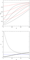Fig. 10.

Top panel: parameter ξ_CIV behavior as a function of viewing angle as a function of θ for a “thin” emitting region with κ = 0.1, for different 𝒬 values (0.4, 1.6, 4.0, 12.0; black lines). Red line: ξ_CIV behavior for a thick emitting region κ = 0.5, for the same 𝒬 values. Bottom panel: as in top panel but for κ = 0.1, with 𝒬 = 12. The thin lines are the $\tilde{ξ}$ $\tilde{\xi}$ values for Hβ (black) and C IVλ1549 (blue). See text for more details. The thick line is their ratio (also shown in the top panel).

The panels of Fig. 11 compare the observed distribution of ξ_CIV, 1 (shaded histogram) with the prediction of randomly oriented synthetic samples, at different 𝒬. We are not seeking a fit of the observed distribution especially around ξ_CIV ≈ 1 because of the many biases affecting our sample and of the problem raised by ξ_CIV > 1 (see below), but a qualitative consistency in the distribution of ξ_CIV < 1.

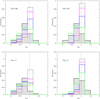Fig. 11.

Top left: observed distribution of ξ_CIV for the full FOS+HE sample (shaded histogram), and distribution of ξ_CIV for 𝒬 = 0.4 (gray), 0.8 (magenta), 2.0 (blue), and 7.8 (green), assuming κ = 0.1, for randomly oriented synthetic samples. Top right: as in top-left panel but for κ = 0.5. Bottom left: distribution of ξ_CIV restricted to Pop. A sources for 𝒬 = 1.0 (gray), 2.0 (magenta), 4.0 (blue), and 12.0 (green), for κ = 0.1. Bottom right: as in bottom-left but for Pop. B sources, with 𝒬 = 0. (gray),0.2 (magenta), 0.4 (blue), and 1.6 (green), for κ = 0.1. See text for more details.

If we focus the analysis of Fig. 11 mainly on large shifts, the presence of low ξ_CIV values and their higher frequency favors a highly flattened low-ionization BLR, as well as high 𝒬 for the full sample. A fat κ = 0.5 BLR is unable to reproduce the largest shift amplitudes. The scatter in ξ_CIV linear values at 𝒬 ≳ 2𝒬 ≳ 2 is ≈0.2, implying a dispersion in the M_BH of ≈0.15 dex. If we separate Pop. A and B, more extreme values of 𝒬 ≳ 2 are required to fit the large shift distribution in Pop. A, with 𝒬 ∼ 10. The distribution of ξ_CIV for Pop. B is more peaked around ξ_CIV ≈ 1, and the ξ_CIV distribution can be qualitatively accounted for if 𝒬 ≲ 2.

The ξ_CIV observed distribution includes values > 1. These values are not possible following our model: the FWHM(C IVλ1549) should be always in excess of or comparable to FWHM(Hβ_BC). In the case of 𝒬 ≫ 1, the C IVλ1549 line is broadened by an outflowing component; if 𝒬 → 0, ξ_CIV ≲ 1. In the latter case, the excess broadening may come from the smaller emissivity-weighted distance expected for C IVλ1549 in a virial velocity field. The existence of cases with FWHM C IVλ1549 < FWHM Hβ was already noted by Mejía-Restrepo et al. (2018b), and therefore it is not unique to the FOS+HE sample. The bottom-right panel of Fig. 11 shows that such cases are relatively frequent among Pop. B. Inspection of the HE spectra in Paper I reveals that the C IVλ1549 profile is significantly affected by semi-broad absorptions such as the ones often found in mini-BAL quasars (Vestergaard 2003; Sulentic et al. 2006b). Since mini-BALs cluster around the line core, it is most likely that these Pop. B sources would satisfy the condition FWHM C IVλ1549 ≳ FWHM Hβ if the effect of the absorptions could be removed.

5.4. M_BH scaling laws dependent on L/L_Edd and L

The goal is to obtain an M_BH estimator based on C IVλ1549 that is consistent with the scaling law derived for Hβ. In this context, the dependence on luminosity of FWHM C IVλ1549 cannot be ignored especially if samples encompass a broad range in luminosity. This will be the case in deep, forthcoming surveys. Considering the corrections to FWHM C IVλ1549 of Sect. 4, the M_BH scaling law is derived in the form log M_BH = α ⋅ log L + 2 ⋅ log FWHM + γ by minimizing the scatter and any systematic deviation of M_BH estimated from C IVλ1549 with respect to the Hβ-derived masses: the unweighted least-square fit of Fig. 12 yields

$\begin{matrix} M_{BH} (CIV) \approx (0.99 \pm 0.04) M_{BH} (H β) + (0.11 \pm 0.39) . \end{matrix}$ $\begin{aligned} M_{\mathrm{BH}}({\mathrm{CIV}}) \approx (0.99 \pm 0.04) M_{\mathrm{BH}}(\mathrm{H}\beta ) + (0.11\pm 0.39). \end{aligned}$ (16)

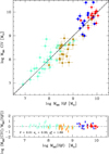Fig. 12.

M_BH computed from the fiducial relation of Vestergaard & Peterson (2006) based on FWHM Hβ vs. the one computed from the C IVλ1549 FWHM corrected following Eq. (6). Error bars include luminosity uncertainties estimated by the scatter in L derived from the UV and the visual spectral ranges along with errors on FWHM propagated quadratically. Lower panel: residuals for the three cases. Meaning of the color-code is the same as in the previous Figs.

The C IVλ1549 scaling law, with M_BH in solar units and L₁₄₅₀ normalized by 10⁴⁴, takes the form:

$\begin{matrix} log M_{BH, 1} CIV \approx & (0 . 64_{- 0.025}^{+ 0.045}) log L_{1450, 44} \\ + 2 log (ξ_{CIV, 1} FWHM (CIV)) + (0 . 525_{- 0.18}^{+ 0.22}) \end{matrix}$ $\begin{aligned} \log M_{\mathrm{BH,1}}\, {\mathrm{CIV}} \approx &(0.64^{+0.045}_{-0.025}) \log L_{1450,44}\nonumber \\&+ 2 \log \left(\xi _{\mathrm{CIV,1}}{{FWHM}}({\mathrm{CIV}}) \right) + (0.525^{+0.22}_{-0.18}) \end{aligned}$ (17)

for the FWHM correction using Eq. (6). Applying Eq. (7), the scaling law does not change appreciably, and uncertainties in the coefficients are only slightly different.

$\begin{matrix} log M_{BH, 2} CIV \approx & (0 . 63_{- 0.035}^{+ 0.045}) log L_{1450, 44} \\ + 2 log (ξ_{CIV, 2} FWHM (CIV)) + (0 . 525_{- 0.19}^{+ 0.275}) . \end{matrix}$ $\begin{aligned} \log M_{\mathrm{BH,2}}\, {\mathrm{CIV}} \approx &(0.63^{+0.045}_{-0.035}) \log L_{1450,44}\nonumber \\&+ 2 \log \left(\xi _{\mathrm{CIV,2}}{\mathrm{FWHM}}({\mathrm{CIV}}) \right) + (0.525^{+0.275}_{-0.19}). \end{aligned}$ (18)

The scaling law parameter uncertainties have been estimated following the standard approach in Bevington & Robinson (2003, p. 210ff), with the constraint that unbiased consistency between M_BH from Hβ and C IVλ1549 (Eq. (16)) is satisfied within the 1σ uncertainties. The rms scatter is σ ≈ 0.33 for Eq. (6) and σ ≈ 0.35 for Eq. (7). Assuming a single correction for both Pop. A and B significantly worsens the fit quality, and no scaling law is reported.

An application of the bisector-fitting technique using SLOPES (Feigelson & Babu 1992) yields

$\begin{matrix} log M_{BH, 1} CIV \approx & (0 . 5925_{- 0.030}^{+ 0.0275}) log L_{1450, 44} \\ + 2 log (ξ_{CIV, 1} FWHM (CIV)) + (0.62 \pm 032), \end{matrix}$ $\begin{aligned} \log M_{\mathrm{BH,1}}\, {\mathrm{CIV}} \approx &(0.5925^{+0.0275}_{-0.030}) \log L_{1450,44} \nonumber \\&+ 2 \log \left(\xi _{\mathrm{CIV,1}}{{FWHM}}({\mathrm{CIV}}) \right) + (0.62\pm 032),\end{aligned}$ (19)

$\begin{matrix} log M_{BH, 2} CIV \approx & (0 . 572_{- 0.032}^{+ 0.0285}) log L_{1450, 44} \\ + 2 log (ξ_{CIV, 2} FWHM (CIV)) + (0.64 \pm 035) . \end{matrix}$ $\begin{aligned} \log M_\mathrm{BH,2} \, \mathrm{CIV} \approx &(0.572^{+0.0285}_{-0.032}) \log L_{1450,44} \nonumber \\&+ 2 \log \left(\xi _\mathrm{CIV,2} {FWHM}(\mathrm{CIV} ) \right) + (0.64\pm 035).\end{aligned}$ (20)

The Vestergaard & Peterson (2006) Hβ scaling laws suffer from significant scatter (see the discussion in their paper) that can be explained on the basis of the scatter induced by orientation (0.33 dex at 1σ) according to the results of Appendix B. The C IVλ1549 and Hβ relation should be considered equivalent. The luminosity exponent (≈0.64) is in agreement with previous observations (Peterson et al. 2005). It is slightly above the exponent of the C IVλ1549 radius dependence on luminosity found in more recent reverberation mapping studies (≈0.52−0.55 Kaspi et al. 2007; Lira et al. 2017, 2018).

Figure 12 suggests the presence of a well-behaved distribution with a few outlying points. It is possible to reduce the scatter to σ ≈ 0.25 applying a σ clipping algorithm (i.e., eliminating all sources deviating more than ±2σ), with no significant change in the best-fit parameters. This selective procedure is however unwarranted: as shown in Appendix C, outlying points are expected precisely because of the possible occurrence of low-probability viewing angles. The residual rms can be largely accounted for by orientation effects if 𝒬 is small, and by the combination of orientation effects and outflow prominence if 𝒬 is much larger than 1 (Appendix C).

5.5. Application to a large sample with Hβ and CIVλ1549 data

The Coatman et al. (2017) data provide a different sample for the testing of the scaling law of Eq. (17). The flux bisector can be converted into $c (\frac{1}{4})$ $c\left(\frac{1}{4}\right)$ (Sect. 4.5). An application of Eq. (17) to Pop. A and B (applying the luminosity-dependent separation as in Paper I) yields agreement with the expectation of an unbiased M_BH estimator with respect to the HβM_BH estimates using the scaling law of Vestergaard & Peterson (2006): the slope of an unweighted least-squares fit is ≈0.958 ± 0.065 (using SLOPES, Feigelson & Babu 1992, Fig. 13).

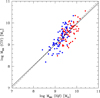Fig. 13.

Estimates of M_BH using corrected C IVλ1549 FWHM as a VBE versus M_BH computed from Hβ FWHM using the scaling law of Vestergaard & Peterson (2006). The luminosity and FWHM(C IVλ1549) data from Coatman et al. (2017) for Pop. A (blue) and B sources (red; see Sect. 5.5 for more details) are used to compute the C IVλ1549 M_BH according to Eq. (17). The dot-dashed line traces the 1:1 relation between M_BH from C IVλ1549 and Hβ; the black line is an unweighted least-squares fit for the A+B M_BH estimates.

6. Conclusion

The present investigation focuses on the C IVλ1549 relations to Hβ over a broad range of luminosities (log L ∼ 43−48, including very high luminosities, log L ≳ 47) in the Eigenvector 1 context, with the goal of testing the C IVλ1549 suitability as virial broadening estimators when observations of low-ionization lines are not available. The Eigenvector 1 context means that the quasar main sequence is considered to properly interpret first-order Eddington ratio effects and luminosity effects that appear to be second order in low- redshift samples.

The main conclusions that we draw from this study are as follows.

1. Within the limits of our sample size, and of our UV spectral coverage, it does not appear that the C IVλ1549 FWHM can be used as a reliable virial broadening estimator without significant corrections. There is large scatter between FWHM measurements on Hβ and C IVλ1549 that seems to defy the definition of a meaningful trend.

2. The C IVλ1549_NC removal improves the agreement between C IVλ1549 and Hβ measurements in the HE sample, but C IVλ1549_NC is not a major factor hampering the definition of a C IVλ1549 VBE consistent with Hβ.

3. Corrections to FWHM C IVλ1549- and C IVλ1549-based M_BH estimates that vary systematically along the 4DE1 sequence and are strongly dependent on Eddington ratio are promising and should be further explored.

4. Following the results of Paper I, we define a correction to the FWHM(C IVλ1549) based on the full-profile C IVλ1549 $c (\frac{1}{2})$ $c\left(\frac{1}{2}\right)$ (a proxy for L/L_Edd) and on the luminosity at 1450 Å. Given the intrinsic differences between Pop. A and B, and their “threshold” separation dependent on a critical L/L_Edd, two different correction laws were considered for the two populations. We note that the correction for Pop. B as derived from the FOS+HE sample is highly uncertain.

5. The M_BH scaling law (Eq. (17)) associated with the corrected FWHM(C IVλ1549) following Eq. (6), as explained in Sect. 5.4, allows for the preservation of the virial dependence on line broadening. Its practical usefulness rests on the ability to distinguish Pop. A and B quasars. This can be achieved in a large fraction of quasars following the guideline set forth by Negrete et al. (2014).

6. We constructed a toy model that helped the interpretation of the scatter. Orientation effects induce scatter ≈0.3−0.4 dex in mass estimates that account for a large fraction of the dispersion in the landmark scaling law of Vestergaard & Peterson (2006). A physical model of the disk + wind system might allow for the viewing angle θ to be recovered for individual quasars.

¹

S/N is measured per pixel on the continuum.

²

If S/N is relatively high ( ≳ 20) only in some peculiar cases might the uncertainty be significantly larger. For example, if the Hβ profile is composed for a narrower core and a broader base, the FWHM measure is unstable, and may abruptly change depending on continuum placement.

³

However, it is not clear whether the results of Runnoe et al. (2014) are applicable to radio quiet quasars: RL sources show no strong evidence of large blueshifts (Sulentic et al. 2007; Richards et al. 2011) as the disk outflow properties may be strongly affected by the powerful radio ejecta (e.g. Punsly 2010; Punsly & Zhang 2011; Sulentic et al. 2015, and references therein).

Acknowledgments

The authors acknowledge the contribution of Jack Sulentic to the development of this paper which is based on observations made with ESO Telescopes at the Paranal Observatory under programme 082.B-0572(A), and with the Italian Telescopio Nazionale Galileo (TNG) operated on the island of La Palma by the Fundación Galileo Galilei of the INAF at the Spanish Observatorio del Roque de los Muchachos of the Instituto de Astrofísica de Canarias.. PM acknowledges the Programa de Estancias de Investigación (PREI) No. DGAP/DFA/2192/2018 of UNAM, where this paper was completed. The relevant research is part of the projects 176001 “Astrophysical spectroscopy of extragalactic objects” and 176003 “Gravitation and structure of universe on large scales” supported by the Ministry of Education, Science and Technological Development of the Republic of Serbia. MLMA acknowledges a CONACyT postdoctoral fellowship, and wishes to thank the IAA for support during her postdoctoral stay from February 2016 to July 2018. MLMA acknowledges a CONACyT postdoctoral fellowship and National Science Centre, Poland, grant No.2017/26/A/ST9/00756 (Maestro 9). AdO and MLMA acknowledge financial support from the Spanish Ministry of Economy and Competitiveness through grant AYA2016-76682-C3-1-P. AdO acknowledges financial support from the State Agency for Research of the Spanish MCIU through the “Center of Excellence Severo Ochoa" award for the Instituto de Astrofísica de Andalucía (SEV-2017-0709). MLMA, PM and MDO acknowledge funding from the INAF PRIN-SKA 2017 program 1.05.01.88.04. DD and AN acknowledge support from CONACyT through grant CB221398. DD also thanks for support from grants IN108715 and IN113719 PAPIIT, DGAPA, UNAM. MAMC was partially supported by the Spanish Research project MTM2015-64095-P and by Diputación General de Aragón, Group E24-17R. The scientific results reported in this article are also based on publicly available HST spectra.

References

Assef, R. J., Denney, K. D., Kochanek, C. S., et al. 2011, ApJ, 742, 93 [NASA ADS] [CrossRef] [Google Scholar]
Bañados, E., Venemans, B. P., Mazzucchelli, C., et al. 2018, Nature, 553, 473 [NASA ADS] [CrossRef] [Google Scholar]
Bachev, R., Marziani, P., Sulentic, J. W., et al. 2004, ApJ, 617, 171 [NASA ADS] [CrossRef] [Google Scholar]
Baldwin, J. A., Ferland, G. J., Korista, K. T., et al. 1996, ApJ, 461, 664 [NASA ADS] [CrossRef] [Google Scholar]
Bensch, K., del Olmo, A., Sulentic, J., Perea, J., & Marziani, P. 2015, JApA, 36, 467 [Google Scholar]
Bevington, P. R., & Robinson, D. K. 2003, Data Reduction and Error Analysis for the Physical Sciences (McGraw-Hill) [Google Scholar]
Bischetti, M., Piconcelli, E., Vietri, G., et al. 2017, A&A, 598, A122 [NASA ADS] [CrossRef] [EDP Sciences] [Google Scholar]
Bisogni, S., di Serego Alighieri, S., Goldoni, P., et al. 2017, A&A, 603, A1 [NASA ADS] [CrossRef] [EDP Sciences] [Google Scholar]
Boller, T., Brandt, W. N., & Fink, H. 1996, A&A, 305, 53 [NASA ADS] [Google Scholar]
Bon, E., Popović, L., & Gavrilović, N. 2007, in Spectral Line Shapes in Astrophysics, eds. L. C. Popovic, & M. S. Dimitrijevic, AIP Conf. Ser., 938, 59 [NASA ADS] [CrossRef] [Google Scholar]
Bon, E., Popović, L. Č., Gavrilović, N., Mura, G. L., & Mediavilla, E. 2009, MNRAS, 400, 924 [NASA ADS] [CrossRef] [Google Scholar]
Bon, N., Bon, E., Marziani, P., & Jovanović, P. 2015, Ap&SS, 360, 7 [CrossRef] [Google Scholar]
Boroson, T. A., & Green, R. F. 1992, ApJS, 80, 109 [NASA ADS] [CrossRef] [Google Scholar]
Boyle, B. J., Shanks, T., Croom, S. M., et al. 2000, MNRAS, 317, 1014 [NASA ADS] [CrossRef] [Google Scholar]
Brotherton, M. S., Wills, B. J., Steidel, C. C., & Sargent, W. L. W. 1994a, ApJ, 423, 131 [NASA ADS] [CrossRef] [Google Scholar]
Brotherton, M. S., Wills, B. J., Francis, P. J., & Steidel, C. C. 1994b, ApJ, 430, 495 [NASA ADS] [CrossRef] [Google Scholar]
Brotherton, M. S., Runnoe, J. C., Shang, Z., & DiPompeo, M. A. 2015, MNRAS, 451, 1290 [NASA ADS] [CrossRef] [Google Scholar]
Burbidge, G. R., & Burbidge, E. M. 1967, Quasi-stellar Objects (San Francisco: Freeman) [Google Scholar]
Chen, K., & Halpern, J. P. 1989, ApJ, 344, 115 [NASA ADS] [CrossRef] [Google Scholar]
Coatman, L., Hewett, P. C., Banerji, M., & Richards, G. T. 2016, MNRAS, 461, 647 [NASA ADS] [CrossRef] [Google Scholar]
Coatman, L., Hewett, P. C., Banerji, M., et al. 2017, MNRAS, 465, 2120 [NASA ADS] [CrossRef] [Google Scholar]
Collin-Souffrin, S., Dyson, J. E., McDowell, J. C., & Perry, J. J. 1988, MNRAS, 232, 539 [NASA ADS] [CrossRef] [Google Scholar]
Corbin, M. R. 1990, ApJ, 357, 346 [NASA ADS] [CrossRef] [Google Scholar]
Corbin, M. R., & Boroson, T. A. 1996, ApJS, 107, 69 [NASA ADS] [CrossRef] [Google Scholar]
Croom, S. M. 2011, ApJ, 736, 161 [NASA ADS] [CrossRef] [Google Scholar]
Czerny, B., & Hryniewicz, K. 2011, A&A, 525, L8 [NASA ADS] [CrossRef] [EDP Sciences] [Google Scholar]
Debuhr, J., Quataert, E., & Ma, C.-P. 2012, MNRAS, 420, 2221 [NASA ADS] [CrossRef] [Google Scholar]
Decarli, R., Dotti, M., & Treves, A. 2011, MNRAS, 413, 39 [NASA ADS] [CrossRef] [Google Scholar]
Denney, K. D., Peterson, B. M., Pogge, R. W., et al. 2010, ApJ, 721, 715 [NASA ADS] [CrossRef] [Google Scholar]
Denney, K. D., Vestergaard, M., Watson, D., & Davis, T. 2012, Am. Astron. Soc. Meeting Abstracts, 219, 440.20 [NASA ADS] [Google Scholar]
Denney, K. D., Pogge, R. W., Assef, R. J., et al. 2013, ApJ, 775, 60 [NASA ADS] [CrossRef] [Google Scholar]
Denney, K. D., Horne, K., Brandt, W. N., et al. 2016, ApJ, 833, 33 [NASA ADS] [CrossRef] [Google Scholar]
Du, P., Lu, K.-X., Hu, C., et al. 2016, ApJ, 820, 27 [NASA ADS] [CrossRef] [Google Scholar]
Du, P., Zhang, Z.-X., Wang, K., et al. 2018, ApJ, 856, 6 [NASA ADS] [CrossRef] [Google Scholar]
Dultzin-Hacyan, D., Taniguchi, Y., & Uranga, L. 1999, in Structure and Kinematics of Quasar Broad Line Regions, eds. C. M. Gaskell, W. N. Brandt, M. Dietrich, D. Dultzin-Hacyan, & M. Eracleous, ASP Conf. Ser., 175, 303 [NASA ADS] [Google Scholar]
Elvis, M. 2000, ApJ, 545, 63 [NASA ADS] [CrossRef] [Google Scholar]
Eracleous, M., & Halpern, J. P. 2004, ApJS, 150, 181 [NASA ADS] [CrossRef] [Google Scholar]
Feigelson, E. D., & Babu, G. J. 1992, ApJ, 397, 55 [NASA ADS] [CrossRef] [Google Scholar]
Ferland, G. J., Hu, C., Wang, J., et al. 2009, ApJ, 707, L82 [NASA ADS] [CrossRef] [Google Scholar]
Fine, S., Croom, S. M., Bland-Hawthorn, J., et al. 2010, MNRAS, 409, 591 [NASA ADS] [CrossRef] [Google Scholar]
Flohic, H. M. L. G., Eracleous, M., & Bogdanović, T. 2012, ApJ, 753, 133 [NASA ADS] [CrossRef] [Google Scholar]
Gallerani, S., Fan, X., Maiolino, R., & Pacucci, F. 2017, PASA, 34, e022 [NASA ADS] [CrossRef] [Google Scholar]
Gaskell, C. M. 1982, ApJ, 263, 79 [NASA ADS] [CrossRef] [Google Scholar]
Goad, M. R., & Korista, K. T. 2014, MNRAS, 444, 43 [NASA ADS] [CrossRef] [Google Scholar]
Grier, C. J., Peterson, B. M., Horne, K., et al. 2013, ApJ, 764, 47 [NASA ADS] [CrossRef] [Google Scholar]
Hall, P. B., Hutsemékers, D., Anderson, S. F., et al. 2003, ApJ, 593, 189 [NASA ADS] [CrossRef] [Google Scholar]
Hewett, P. C., & Wild, V. 2010, MNRAS, 405, 2302 [NASA ADS] [Google Scholar]
Hu, C., Wang, J.-M., Ho, L. C., et al. 2008, ApJ, 683, L115 [NASA ADS] [CrossRef] [Google Scholar]
Hu, C., Wang, J.-M., Ho, L. C., et al. 2012, ApJ, 760, 126 [NASA ADS] [CrossRef] [Google Scholar]
Karouzos, M., Woo, J.-H., Matsuoka, K., et al. 2015, ApJ, 815, 128 [NASA ADS] [CrossRef] [Google Scholar]
Kaspi, S., Brandt, W. N., Maoz, D., et al. 2007, ApJ, 659, 997 [NASA ADS] [CrossRef] [Google Scholar]
Kelly, B. C., & Bechtold, J. 2007, ApJS, 168, 1 [NASA ADS] [CrossRef] [Google Scholar]
Kollatschny, W., & Zetzl, M. 2013, A&A, 549, A100 [NASA ADS] [CrossRef] [EDP Sciences] [Google Scholar]
Kriss, G. 1994, ASP Conf. Ser., 61, 437 [Google Scholar]
Kuraszkiewicz, J., Wilkes, B. J., Schmidt, G., et al. 2009, ApJ, 692, 1180 [NASA ADS] [CrossRef] [Google Scholar]
Kwan, J., & Krolik, J. H. 1981, ApJ, 250, 478 [NASA ADS] [CrossRef] [Google Scholar]
Laor, A., Fiore, F., Elvis, M., Wilkes, B. J., & McDowell, J. C. 1997, ApJ, 477, 93 [NASA ADS] [CrossRef] [Google Scholar]
Latif, M. A., & Ferrara, A. 2016, PASA, 33, e051 [NASA ADS] [CrossRef] [Google Scholar]
Leighly, K. M. 2004, ApJ, 611, 125 [NASA ADS] [CrossRef] [Google Scholar]
Lira, P., Botti, I., Kaspi, S., & Netzer, H. 2017, Front. Astron. Space Sci., 4, 71 [NASA ADS] [CrossRef] [Google Scholar]
Lira, P., Kaspi, S., Netzer, H., et al. 2018, ApJ, 865, 56 [NASA ADS] [CrossRef] [Google Scholar]
Martínez-Aldama, M. L., Dultzin, D., Marziani, P., et al. 2015, ApJS, 217, 3 [NASA ADS] [CrossRef] [Google Scholar]
Martínez-Aldama, M. L., Del Olmo, A., Marziani, P., et al. 2018, Front. Astron. Space Sci., 4, 65 [NASA ADS] [CrossRef] [Google Scholar]
Marziani, P., Sulentic, J. W., Dultzin-Hacyan, D., Calvani, M., & Moles, M. 1996, ApJS, 104, 37 [Google Scholar]
Marziani, P., Sulentic, J. W., Zamanov, R., et al. 2003, ApJS, 145, 199 [NASA ADS] [CrossRef] [Google Scholar]
Marziani, P., Sulentic, J. W., Negrete, C. A., et al. 2010, MNRAS, 409, 1033 [NASA ADS] [CrossRef] [Google Scholar]
Marziani, P., Sulentic, J. W., Plauchu-Frayn, I., & del Olmo, A. 2013a, ApJ, 764, 150 [NASA ADS] [CrossRef] [Google Scholar]
Marziani, P., Sulentic, J. W., Plauchu-Frayn, I., & del Olmo, A. 2013b, A&A, 555, A89 [NASA ADS] [CrossRef] [EDP Sciences] [Google Scholar]
Marziani, P., Martínez Carballo, M. A., Sulentic, J. W., et al. 2016, Ap&SS, 361, 29 [NASA ADS] [CrossRef] [Google Scholar]
Marziani, P., Dultzin, D., Sulentic, J. W., et al. 2018, Front. Astron. Space Sci., 5, 6 [CrossRef] [Google Scholar]
Matsuoka, Y., Kawara, K., & Oyabu, S. 2008, ApJ, 673, 62 [NASA ADS] [CrossRef] [Google Scholar]
Matsuoka, K., Silverman, J. D., Schramm, M., et al. 2013, ApJ, 771, 64 [NASA ADS] [CrossRef] [Google Scholar]
McLure, R. J., & Dunlop, J. S. 2004, MNRAS, 352, 1390 [NASA ADS] [CrossRef] [Google Scholar]
McLure, R. J., & Jarvis, M. J. 2002, MNRAS, 337, 109 [NASA ADS] [CrossRef] [Google Scholar]
Mejía-Restrepo, J. E., Trakhtenbrot, B., Lira, P., Netzer, H., & Capellupo, D. M. 2016, MNRAS, 460, 187 [NASA ADS] [CrossRef] [Google Scholar]
Mejía-Restrepo, J. E., Lira, P., Netzer, H., Trakhtenbrot, B., & Capellupo, D. 2017, Front. Astron. Space Sci., 4, 70 [NASA ADS] [CrossRef] [Google Scholar]
Mejía-Restrepo, J. E., Lira, P., Netzer, H., Trakhtenbrot, B., & Capellupo, D. M. 2018a, Nat. Astron., 2, 63 [NASA ADS] [CrossRef] [Google Scholar]
Mejía-Restrepo, J. E., Trakhtenbrot, B., Lira, P., & Netzer, H. 2018b, MNRAS, 478, 1929 [NASA ADS] [CrossRef] [Google Scholar]
Negrete, C. A., Dultzin, D., Marziani, P., & Sulentic, J. W. 2014, ApJ, 794, 95 [NASA ADS] [CrossRef] [Google Scholar]
Negrete, C. A., Dultzin, D., Marziani, P., et al. 2017, Front. Astron. Space Sci., 4, 59 [NASA ADS] [CrossRef] [Google Scholar]
Negrete, C. A., Dultzin, D., Marziani, P., et al. 2018, A&A, 620, A118 [NASA ADS] [CrossRef] [EDP Sciences] [Google Scholar]
Netzer, H. 1990, in Active Galactic Nuclei, eds. R. D. Blandford, H. Netzer, L. Woltjer, T. J.-L. Courvoisier, & M. Mayor, 57 [Google Scholar]
Netzer, H., & Marziani, P. 2010, ApJ, 724, 318 [NASA ADS] [CrossRef] [Google Scholar]
Netzer, H., Lira, P., Trakhtenbrot, B., Shemmer, O., & Cury, I. 2007, ApJ, 671, 1256 [NASA ADS] [CrossRef] [Google Scholar]
Osterbrock, D. E., & Shuder, J. M. 1982, ApJS, 49, 149 [NASA ADS] [CrossRef] [Google Scholar]
Park, D., Woo, J.-H., Denney, K. D., & Shin, J. 2013, ApJ, 770, 87 [NASA ADS] [CrossRef] [Google Scholar]
Pei, L., Fausnaugh, M. M., Barth, A. J., et al. 2017, ApJ, 837, 131 [NASA ADS] [CrossRef] [Google Scholar]
Peterson, B. M. 2014, SpScieRev, 183, 253 [Google Scholar]
Peterson, B. M., & Ferland, G. J. 1986, Nature, 324, 345 [NASA ADS] [CrossRef] [Google Scholar]
Peterson, B. M., & Wandel, A. 1999, ApJ, 521, L95 [NASA ADS] [CrossRef] [Google Scholar]
Peterson, B. M., & Wandel, A. 2000, ApJ, 540, L13 [NASA ADS] [CrossRef] [Google Scholar]
Peterson, B. M., Bentz, M. C., Desroches, L.-B., et al. 2005, ApJ, 632, 799 [NASA ADS] [CrossRef] [Google Scholar]
Plotkin, R. M., Shemmer, O., Trakhtenbrot, B., et al. 2015, ApJ, 805, 123 [NASA ADS] [CrossRef] [Google Scholar]
Proga, D., & Kallman, T. R. 2004, ApJ, 616, 688 [Google Scholar]
Proga, D., Stone, J. M., & Kallman, T. R. 2000, ApJ, 543, 686 [NASA ADS] [CrossRef] [Google Scholar]
Punsly, B. 2010, ApJ, 713, 232 [NASA ADS] [CrossRef] [Google Scholar]
Punsly, B., & Zhang, S. 2011, ApJ, 735, L3 [NASA ADS] [CrossRef] [Google Scholar]
Richards, G. T., Kruczek, N. E., Gallagher, S. C., et al. 2011, AJ, 141, 167 [NASA ADS] [CrossRef] [Google Scholar]
Runnoe, J. C., Brotherton, M. S., DiPompeo, M. A., & Shang, Z. 2014, MNRAS, 438, 3263 [NASA ADS] [CrossRef] [Google Scholar]
Saito, Y., Imanishi, M., Minowa, Y., et al. 2016, PASJ, 68, 1 [NASA ADS] [CrossRef] [Google Scholar]
Sdowski, A., Narayan, R., McKinney, J. C., & Tchekhovskoy, A. 2014, MNRAS, 439, 503 [NASA ADS] [CrossRef] [Google Scholar]
Shang, Z., Brotherton, M. S., Wills, B. J., et al. 2011, ApJS, 196, 2 [NASA ADS] [CrossRef] [Google Scholar]
Shen, Y. 2013, Bull. Astron. Soc. India, 41, 61 [NASA ADS] [Google Scholar]
Shen, Y. 2016, ApJ, 817, 55 [NASA ADS] [CrossRef] [Google Scholar]
Shen, Y., & Ho, L. C. 2014, Nature, 513, 210 [NASA ADS] [CrossRef] [Google Scholar]
Shen, Y., & Liu, X. 2012, ApJ, 753, 125 [NASA ADS] [CrossRef] [Google Scholar]
Shen, Y., Brandt, W. N., Richards, G. T., et al. 2016, ApJ, 831, 7 [NASA ADS] [CrossRef] [Google Scholar]
Snedden, S., & Gaskell, C. 2004, in AGN Physics with the Sloan Digital Sky Survey, eds. G. T. Richards, & P. B. Hall, ASP Conf. Ser., 311, 197 [NASA ADS] [Google Scholar]
Snedden, S. A., & Gaskell, C. M. 2007, ApJ, 669, 126 [NASA ADS] [CrossRef] [Google Scholar]
Steinhardt, C. L., & Silverman, J. D. 2013, PASJ, 65, 82 [NASA ADS] [CrossRef] [Google Scholar]
Stevens, I. R., & Kallman, T. R. 1990, ApJ, 365, 321 [NASA ADS] [CrossRef] [Google Scholar]
Storchi-Bergmann, T., Schimoia, J. S., Peterson, B. M., et al. 2017, ApJ, 835, 236 [NASA ADS] [CrossRef] [Google Scholar]
Strateva, I. V., Strauss, M. A., Hao, L., et al. 2003, AJ, 126, 1720 [NASA ADS] [CrossRef] [Google Scholar]
Sulentic, J. W. 1989, ApJ, 343, 54 [NASA ADS] [CrossRef] [Google Scholar]
Sulentic, J., & Marziani, P. 2015, Front. Astron. Space Sci., 2, 6 [NASA ADS] [CrossRef] [Google Scholar]
Sulentic, J. W., Marziani, P., & Dultzin-Hacyan, D. 2000a, ARA&A, 38, 521 [NASA ADS] [CrossRef] [Google Scholar]
Sulentic, J. W., Marziani, P., Zwitter, T., Dultzin-Hacyan, D., & Calvani, M. 2000b, ApJ, 545, L15 [NASA ADS] [CrossRef] [Google Scholar]
Sulentic, J. W., Zwitter, T., Marziani, P., & Dultzin-Hacyan, D. 2000c, ApJ, 536, L5 [NASA ADS] [CrossRef] [Google Scholar]
Sulentic, J. W., Marziani, P., Zamanov, R., et al. 2002, ApJ, 566, L71 [NASA ADS] [CrossRef] [Google Scholar]
Sulentic, J. W., Stirpe, G. M., Marziani, P., et al. 2004, A&A, 423, 121 [NASA ADS] [CrossRef] [EDP Sciences] [Google Scholar]
Sulentic, J. W., Repetto, P., Stirpe, G. M., et al. 2006a, A&A, 456, 929 [NASA ADS] [CrossRef] [EDP Sciences] [Google Scholar]
Sulentic, J. W., Dultzin-Hacyan, D., Marziani, P., et al. 2006b, Rev. Mex. Astron. Astrofis., 42, 23 [NASA ADS] [Google Scholar]
Sulentic, J. W., Bachev, R., Marziani, P., Negrete, C. A., & Dultzin, D. 2007, ApJ, 666, 757 [NASA ADS] [CrossRef] [Google Scholar]
Sulentic, J., Marziani, P., & Zamfir, S. 2011, Balt. Astron., 20, 427 [NASA ADS] [Google Scholar]
Sulentic, J. W., Marziani, P., del Olmo, A., et al. 2014, A&A, 570, A96 [NASA ADS] [CrossRef] [EDP Sciences] [Google Scholar]
Sulentic, J. W., Martínez-Carballo, M. A., Marziani, P., et al. 2015, MNRAS, 450, 1916 [NASA ADS] [CrossRef] [Google Scholar]
Sulentic, J. W., del Olmo, A., Marziani, P., et al. 2017, A&A, 608, A122 [NASA ADS] [CrossRef] [EDP Sciences] [Google Scholar]
Sun, J., & Shen, Y. 2015, ApJ, 804, L15 [NASA ADS] [CrossRef] [Google Scholar]
Sun, M., Xue, Y., Richards, G. T., et al. 2018, ApJ, 854, 128 [NASA ADS] [CrossRef] [Google Scholar]
Tilton, E. M., & Shull, J. M. 2013, ApJ, 774, 67 [NASA ADS] [CrossRef] [Google Scholar]
Trakhtenbrot, B., & Netzer, H. 2012, MNRAS, 427, 3081 [NASA ADS] [CrossRef] [Google Scholar]
Trevese, D., Perna, M., Vagnetti, F., Saturni, F. G., & Dadina, M. 2014, ApJ, 795, 164 [NASA ADS] [CrossRef] [Google Scholar]
Tytler, D., & Fan, X.-M. 1992, ApJS, 79, 1 [NASA ADS] [CrossRef] [Google Scholar]
Vanden Berk, D. E., Richards, G. T., Bauer, A., et al. 2001, AJ, 122, 549 [NASA ADS] [CrossRef] [Google Scholar]
Vestergaard, M. 2003, ApJ, 599, 116 [NASA ADS] [CrossRef] [Google Scholar]
Vestergaard, M., & Peterson, B. M. 2006, ApJ, 641, 689 [NASA ADS] [CrossRef] [Google Scholar]
Vietri, G. 2017, Am. Astron. Soc. Meeting Abstracts, 229, 302.06 [NASA ADS] [Google Scholar]
Vietri, G., Piconcelli, E., Bischetti, M., et al. 2018, A&A, 617, A81 [NASA ADS] [CrossRef] [EDP Sciences] [Google Scholar]
Vollmer, B., Schartmann, M., Burtscher, L., et al. 2018, A&A, 615, A164 [NASA ADS] [CrossRef] [EDP Sciences] [Google Scholar]
Wang, J., & Li, Y. 2011, ApJ, 742, L12 [NASA ADS] [CrossRef] [Google Scholar]
Wang, T., Brinkmann, W., & Bergeron, J. 1996, A&Ap, 309, 81 [NASA ADS] [Google Scholar]
Wang, J., Dong, X., Wang, T., et al. 2009, ApJ, 707, 1334 [NASA ADS] [CrossRef] [Google Scholar]
Wang, H., Wang, T., Zhou, H., et al. 2011, ApJ, 738, 85 [NASA ADS] [CrossRef] [Google Scholar]
Wang, J.-M., Qiu, J., Du, P., & Ho, L. C. 2014a, ApJ, 797, 65 [NASA ADS] [CrossRef] [Google Scholar]
Wang, J.-M., Du, P., Li, Y.-R., et al. 2014b, ApJ, 792, L13 [NASA ADS] [CrossRef] [Google Scholar]
Wang, J.-M., Du, P., Brotherton, M. S., et al. 2017, Nat. Astron., 1, 775 [NASA ADS] [CrossRef] [Google Scholar]
Wills, B. J., Netzer, H., & Wills, D. 1985, ApJ, 288, 94 [NASA ADS] [CrossRef] [Google Scholar]
Wills, B. J., Brotherton, M. S., Fang, D., Steidel, C. C., & Sargent, W. L. W. 1993, ApJ, 415, 563 [NASA ADS] [CrossRef] [Google Scholar]
Wisotzki, L., Christlieb, N., Bade, N., et al. 2000, A&A, 358, 77 [NASA ADS] [Google Scholar]
Yip, C. W., Connolly, A. J., Vanden Berk, D. E., et al. 2004, AJ, 128, 2603 [NASA ADS] [CrossRef] [Google Scholar]
Yong, S. Y., King, A. L., Webster, R. L., et al. 2018, MNRAS, 479, 4153 [NASA ADS] [CrossRef] [Google Scholar]
Zamanov, R., Marziani, P., Sulentic, J. W., et al. 2002, ApJ, 576, L9 [NASA ADS] [CrossRef] [Google Scholar]
Zamfir, S., Sulentic, J. W., Marziani, P., & Dultzin, D. 2010, MNRAS, 403, 1759 [NASA ADS] [CrossRef] [Google Scholar]

Appendix A: The MS / 4DE1 formalism: a glossary

In the optical plane of the quasar main sequence, spectral types are isolated following Sulentic et al. (2002). Figure A.1 provides a sketch and Table A.1 a summary with the spectral types identification in the optical plane of the MS. Here we provide a glossary of the MS-related terms and acronyms employed in the paper, along the order of the quasar main sequence. A more thorough description can be found in Sulentic et al. (2011) and Marziani et al. (2018).

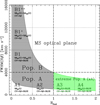Fig. A.1.

Schematic representation of the optical plane of the quasar MS, with the subdivisions identifying spectral types along the sequence. The main components that are blended in the Hβ and C IVλ1549 profile are listed in each spectral bin. The shaded area shows the approximate occupation of low-z quasars sample in the plane.

Table A.1.

Spectral type definition along the main sequence.

The rational for two type-1 quasar populations (A and B) was originally given by Sulentic et al. (2000a). Spectral types A3 and A4 are also indicated as extreme Population A, with R_FeII ≳ 1. They are the highest radiators per unit mass and possibly super-Eddington accretors (Wang et al. 2014b).

The 4D Eigenvector-1 formalism was introduced to limit the set of MS-correlated parameters to the four ones that are most relevant for the MS physical interpretation. In addition to FWHM Hβ, R_FeII, and $c (\frac{1}{2})$ $c\left(\frac{1}{2}\right)$ C IVλ1549, the soft X-ray photon index Γ_soft is also considered (Sulentic et al. 2000b). The four parameters were meant to represent the velocity dispersion of the LIL-emitting part of the BLR, the physical condition within the LIL-BLR (R_FeII), the dynamical condition of the HIL-emitting gas, and the accretion state of the black hole. Γ_soft > 2 implies a soft X-ray excess that is exclusive of Population A (Wang et al. 1996; Boller et al. 1996; Shen & Ho 2014; Bensch et al. 2015).

Line components assumed in the decomposition along the MS are defined as follows (see also the sketch of Fig. A.1 and Table A.2).

Table A.2.

Line components along the main sequence.

BLUE becomes detectable as a blueward excess in the Hβ profile mainly in A3 and A4 (more infrequently in A2). For C IVλ1549, BLUE increases in prominence along the sequence from B1⁺⁺, to A4. In B1⁺⁺ and B1⁺ is weak and often undetectable, while in A3 and A4 it may dominate C IVλ1549 emission.

Appendix B: Effect of orientation on HβM_BH estimates

From the inversion of Eq. (9), we obtain an expression for the viewing angle $θ = arcsin \sqrt{x^{2} / 4 - κ^{2}}$ $\theta = \arcsin{\sqrt{x^2/4 - \kappa^2}}$ , where x = δν_obs/δν_K and κ = δν_iso/δν_K. The probability to observe δν_obs for a given δν_K is then

$\begin{matrix} P (x) = \sqrt{x^{2} / 4 - κ^{2}} \frac{d θ}{d x} = \frac{x / 4}{\sqrt{κ^{2} - x^{2} / 4 + 1}} \cdot \end{matrix}$ $\begin{aligned} P(x) = \sqrt{x^2/4-\kappa ^{2}} \frac{\mathrm{d}\theta }{\mathrm{d}x} = \frac{x/4}{\sqrt{\kappa ^2-x^2/4+1}}\cdot \end{aligned}$ (B.1)

The black hole mass is ∝x². Therefore the average effect can be written as

$\begin{matrix} ⟨ \frac{M_{BH, obs}}{M_{BH, K}} ⟩ = \int_{x (ν_{iso})}^{x (edge)} x^{2} P (x) d x / \int_{x (ν_{iso})}^{x (edge)} P (x) d x . \end{matrix}$ $\begin{aligned} \langle \frac{M_\mathrm{BH,obs} }{M_\mathrm{BH,K} }\rangle = \int _{x(\nu _\mathrm{iso} )}^{x(\mathrm{edge} )} x^2 P(x) \mathrm{d}x{ /} \int _{x(\nu _\mathrm{iso} )}^{x(\mathrm{edge} )} P(x) \mathrm{d}x. \end{aligned}$ (B.2)

The integrals of Eq. (B.2) can be computed analytically:

$\begin{matrix} \int x^{2} P (x) d x = & (- \frac{4}{3} \sqrt{4 κ^{2} - x^{2} + 4}) \\ - \frac{4}{3} κ^{2} \sqrt{4 κ^{2} - x^{2} + 4} - \frac{1}{6} (x^{2} \sqrt{4 κ^{2} - x^{2} + 4}), \end{matrix}$ $\begin{aligned} \int x^2 P(x)\mathrm{d}x =&\left(-\frac{4}{3}\sqrt{4\kappa ^2-x^2+4}\right)\\& -\frac{4}{3}\kappa ^2 \sqrt{4\kappa ^2-x^2+4} -\frac{1}{6}\left(x^2 \sqrt{4\kappa ^2-x^2+4}\right),\nonumber \end{aligned}$ (B.3)

$\begin{matrix} \int P (x) d x = - \sqrt{1 + κ^{2} - x^{2} / 4} . \end{matrix}$ $\begin{aligned} \int P(x) \mathrm{d}x = -\sqrt{1+ \kappa ^2 - x^2/4}. \end{aligned}$ (B.4)

We note that the integration limits in x (which correspond to θ = 0 and θ = 45) are different for κ = 0.1 and 0.5. For κ = 0.1, x_iso = 0.2 and x_edge ≈ 1.43 In the latter case, θ = 0 corresponds to x_min = 1 and θ = 45 to x_edge ≈ 1.73: M_BH will be always overestimated, for every possible θ value larger than 0.

If we consider the Eddington ratio, we obtain

$\begin{matrix} \int P (x) / x^{2} d x = - arctan h (\frac{\sqrt{κ^{2} + 1}}{\sqrt{κ^{2} - x^{2} / 4 + 1}}) / 4 \sqrt{κ^{2} + 1} . \end{matrix}$ $\begin{aligned} \int P(x)/x^2 \mathrm{d}x= -\arctan {\mathrm{h} } \left(\frac{\sqrt{\kappa ^2+1}}{\sqrt{\kappa ^2-x^2/4+1}}\right)/4{\sqrt{\kappa ^2+1}} . \end{aligned}$ (B.5)

Equation (B.5) implies a significant effect on L/L_Edd for both κ = 0.1 and κ = 0.5. In the first case, the L/L_Edd will be overestimated by a factor ≈1.8. In the second case, the L/L_Edd will be underestimated by a factor ≈2, due to the systematic overestimation in M_BH.

Appendix C: Origin of scatter in scaling laws

We considered synthetic samples of ∼10 000 objects obtained from random variates with distribution P(θ)∝sinθ (0 ≤ θ ≤ π/4), and “true” M_BH uniformly distributed in the range 10⁷ M_⊙ ≤ M_BH ≤ 10⁹ M_⊙. The dependence on orientation of the Hβ FWHM is assumed to follow Eq. (9), with κ = 0.1. The effect of orientation on FWHM is such that in a randomly oriented synthetic sample the M_BH estimated from Hβ deviates from the true M_BH as in Fig. C.1 (top panel). The dispersion is ≈0.35, which is comparable to the uncertainty in the scaling-law M_BH estimate following Vestergaard & Peterson (2006, ≈0.5 at 1σ confidence level).

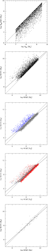Fig. C.1.

Top: M_BH with effect of orientation via Eq. (10) vs. the “true” M_BH, for a synthetic sample of 10 000 sources. Second from top: M_BH C IVλ1549 vs. M_BH Hβ estimated for an Eddington ratio distribution as described in the text and no correction. Third from top: FWHM M_BH C IVλ1549 corrected because of outflow broadening using a correction factor ξ. The blue dots identify the M_BH Hβ estimates that are under 0.33 dex the true M_BH; the red ones are for overestimates by more than 0.33 dex. The gray dots represent mass estimates within −0.33 and +0.33 dex from the true value. Fourth from top: as above but with color-coding referring to C IVλ1549 M_BH. Bottom: synthetic sample with n ≲ 80 sources, as in the FOS+HE sample. See text for more details. In all panels, the dot-dashed line is the equality line; the filled line traces an unweighted least-squares fit.

The estimates of M_BH C IVλ1549 show a significant scatter if plotted against M_BH Hβ (Fig. 12). The origin of the scatter is in part related to orientation, in part to the outflow component. The second panel from top of Fig. C.1 shows the M_BH C IVλ1549 vs. Hβ for a synthetic sample to which no correction has been applied. FWHM of C IVλ1549 and Hβ are expected to be related to the Keplerian velocity by Eqs. (12) and (10), respectively. The distribution of L/L_Edd has been assumed Gaussian, peaking at log L/L_Edd = −0.3, and σ ≈ 0.5. Typical values of ξ_CIV and 𝒬 are appropriate for Pop. A sources. There is a strong bias (0.5 dex) and a standard deviation of the mass ratios of ≈0.6 dex. In some rare instances (a combination of face-on orientation and large outflow velocity) the ratio between M_BH from Hβ and C IVλ1549 can reach a factor ∼10², as actually found by Sulentic et al. (2007).

The third and fourth panels from the top show the same configuration, but after applying a correction factor ξ_CIV in the form 1/ζ(L, L/L_Edd) = 1/(1 + kL^a(L/L_Edd)^b), with a ≈ 0.1, b ≈ 1 and no dependence on orientation, intended to mimic the correction actually applied to the data in Sect. 4. The orientation effect is changing the C IVλ1549 FWHM following Eq. (12), and therefore displacing the M_BH from the true mass also after correcting the FWHM. We note that the outlying blue points are due to Hβ underestimates of the mass by more than 0.33 dex because of low values of the viewing angle θ. On the contrary, the relatively high value of 𝒬 in the simulation produces a significant fraction of M_BH C IVλ1549 which are overestimating the M_BH by more than 0.33 dex (red points). The dispersion is however reduced with respect to the case with no correction, with an rms ≈ 0.3. The bottom panel is a realization of the synthetic sample for a number of sources ≲100, comparable to the size of the FOS+HE sample, and Gaussian distribution of L/L_Edd as for case shown and correction in the second panel from top.

In all of these cases save the one of the second panel from top the dispersion remains ∼0.3, comparable to the one measured for the scaling laws of Eqs. (17) and (18). It is interesting to note that in the framework of the toy model, if 𝒬 = 0 the orientation-induced scatter is the same for Hβ and C IVλ1549; if 𝒬 ≈ 4, C IVλ1549 becomes an almost perfect VBE, with all the scatter being due to Hβ, in a plot M_BH C IVλ1549 vs M_BH Hβ. These results may be consistent with no strong dependence on orientation of the C IVλ1549 line shift in RL quasars (Runnoe et al. 2014)³.

A uniform distribution of 𝒬 between 0 and 1.6, a situation more appropriate for Pop. B, was also considered. The results were similar with smaller dispersion and biases.

All Tables

Table 1.

Fits of ξ_CIV.

In the text

Table A.1.

Spectral type definition along the main sequence.

In the text

Table A.2.

Line components along the main sequence.

In the text

All Figures

	Fig. 1. Cumulative distribution of bolometric luminosity L of the FOS+HE sample (black), Pop. A (blue), and Pop. B (red).
In the text

Fig. 2.

Virial broadening estimators based on Hβ, with several corrections applied to the HE sample. Top square panel: FWHM Hβ_BC (blue (Pop. A) and red (Pop. B)) with error bars, symmetrized FWHM Hβ (symm, black), and FWHM Hβ corrected according to spectral type (st, aquamarine and dark orange for Pop. A and B respectively) versus FWHM of the full Hβ profile. The gray line traces the correction (corr) following the relation of Sulentic et al. (2006a) reported in Sect. 4. Middle panels: ratios of FWHM after various corrections vs. full profile FWHM. Panels from top show: BC/symm, BC/st, BC/corr, symm/ st, corr/st. Average values, standard deviation and normalized $χ_{ν}^{2}$ $\chi^{2}_{\nu}$ are reported in the upper-right corner of the panels. Bottom square panel: BC, spectral type st and reverberation corrected (corr, open symbols) FWHM values vs. symmetrized FWHM.

In the text

Fig. 3.

Top panel: FWHM(C IVλ1549) vs. FWHM(Hβ) (full profiles) for the FOS+HE sample. Data points are color-coded according to sample and population: HE Pop. A – blue circles (), HE Pop. B – red squares (), FOS Pop. A – aquamarine circles (), and FOS Pop. B – golden squares (). Best fitting least-square lines (dashed) are shown in blue for all Pop. A and red for all Pop. B. The black dot-dashed line is the equality line. The continuous gray line is the expected FWHM following the correction of Sulentic et al. (2006a, corr). Lower panel: ratio between FWHM C IVλ1549 and FWHM Hβ as a function of FWHM (Hβ).

In the text

	Fig. 4. Relation between the logarithm of the FWHM ratio of C IVλ1549 to Hβ and the logarithm of the Eddington ratio L/L_Edd. The vertical dot-dashed line traces the Eddington limit. The colors and shapes of symbols are as in Fig. 3. The dashed line is an unweighted least-squares fit, and the filled line was obtained with the bisector method (Feigelson & Babu 1992).
In the text

	Fig. 5. Top panel: bisector flux estimator of Coatman et al. (2017) vs. $c (\frac{1}{4})$ $c\left(\frac{1}{4}\right)$ , in km s⁻¹. The dot-dashed line is the equality line. Bottom panel: percentage residuals. The shaded areas indicate the average errors of measurements at a 2σ confidence level computed from Table 4 of Paper I.
In the text

	Fig. 6. Top panel: FWHM(C IVλ1549) `C16` (i.e., corrected following Coatman et al. 2016), vs. FWHM(Hβ) `st` for the FOS+HE sample. Meaning of symbols is the same as for Fig. 3. The black dot-dashed line is the equality line. Bottom panel: residuals. Average ratio, dispersion, and $χ_{ν}^{2}$ $\chi^{2}_{\nu}$ refer to all sources.
In the text

	Fig. 7. Top left panel: ξ_CIVFWHM(C IVλ1549) i.e., FWHM(C IVλ1549) after correction for blueshift and luminosity dependence following Eq. (6) vs. FWHM(Hβ) `cm` for the FOS+HE sample. The black dot-dashed line is the equality line, and the meaning of the color-coding is the same as in Fig. 3. Top right: as in top panel but with ξ_CIV computed from Eq. (7).
In the text

Fig. 8.

Black hole mass computed from the fiducial relation of Vestergaard & Peterson (2006) based on FWHM Hβ vs. the ones computed from the C IVλ1549 FWHM following Park et al. (2013), for Pop. A (blue) and B (red) HE sources. Values of M_BH obtained from the Vestergaard & Peterson (2006) C IVλ1549 scaling law after the correction suggested by Brotherton et al. (2015, small dots) are shown by small open circles. Lower panel: residuals as a function of M_BH. The average and the scatter reported for Populations A and B refer to the Park et al. (2013) scaling laws.

In the text

Fig. 9.

Hβ and C IVλ1549 profile parameter comparison as a function of luminosity. Top panels: behavior of FWHM C IVλ1549 and Hβ (upper half) and of the ratio FWHM(C IVλ1549)/FWHM(Hβ) as a function of L (lower half), for FOS (golden and pale blue) and HE sample (red and blue). The yellow band identifies the region where FWHM(C IVλ1549)/FWHM(Hβ) = 1 within the errors. Middle panels: $c (\frac{1}{2})$ $c\left(\frac{1}{2}\right)$ of Hβ and C IVλ1549 (upper half), and difference $δ (\frac{1}{2})$ $\delta\left(\frac{1}{2}\right)$ as a function of L (lower half). Square symbols indicate Pop. B, circles Pop. A. Lines trace an unweighted least-squares fit for the Pop. A (black) and for Pop. B (red) sources. Bottom panels: as in top panels but for $c (\frac{1}{4})$ $c\left(\frac{1}{4}\right)$ and $δ (\frac{1}{4})$ $\delta\left(\frac{1}{4}\right)$ . The vertical dotted lines join Hβ and C IVλ1549 parameters for the same object (e.g., they are not error bars).

In the text

Fig. 10.

Top panel: parameter ξ_CIV behavior as a function of viewing angle as a function of θ for a “thin” emitting region with κ = 0.1, for different 𝒬 values (0.4, 1.6, 4.0, 12.0; black lines). Red line: ξ_CIV behavior for a thick emitting region κ = 0.5, for the same 𝒬 values. Bottom panel: as in top panel but for κ = 0.1, with 𝒬 = 12. The thin lines are the $\tilde{ξ}$ $\tilde{\xi}$ values for Hβ (black) and C IVλ1549 (blue). See text for more details. The thick line is their ratio (also shown in the top panel).

In the text

Fig. 11.

Top left: observed distribution of ξ_CIV for the full FOS+HE sample (shaded histogram), and distribution of ξ_CIV for 𝒬 = 0.4 (gray), 0.8 (magenta), 2.0 (blue), and 7.8 (green), assuming κ = 0.1, for randomly oriented synthetic samples. Top right: as in top-left panel but for κ = 0.5. Bottom left: distribution of ξ_CIV restricted to Pop. A sources for 𝒬 = 1.0 (gray), 2.0 (magenta), 4.0 (blue), and 12.0 (green), for κ = 0.1. Bottom right: as in bottom-left but for Pop. B sources, with 𝒬 = 0. (gray),0.2 (magenta), 0.4 (blue), and 1.6 (green), for κ = 0.1. See text for more details.

In the text

Fig. 12.

M_BH computed from the fiducial relation of Vestergaard & Peterson (2006) based on FWHM Hβ vs. the one computed from the C IVλ1549 FWHM corrected following Eq. (6). Error bars include luminosity uncertainties estimated by the scatter in L derived from the UV and the visual spectral ranges along with errors on FWHM propagated quadratically. Lower panel: residuals for the three cases. Meaning of the color-code is the same as in the previous Figs.

In the text

Fig. 13.

Estimates of M_BH using corrected C IVλ1549 FWHM as a VBE versus M_BH computed from Hβ FWHM using the scaling law of Vestergaard & Peterson (2006). The luminosity and FWHM(C IVλ1549) data from Coatman et al. (2017) for Pop. A (blue) and B sources (red; see Sect. 5.5 for more details) are used to compute the C IVλ1549 M_BH according to Eq. (17). The dot-dashed line traces the 1:1 relation between M_BH from C IVλ1549 and Hβ; the black line is an unweighted least-squares fit for the A+B M_BH estimates.

In the text

	Fig. A.1. Schematic representation of the optical plane of the quasar MS, with the subdivisions identifying spectral types along the sequence. The main components that are blended in the Hβ and C IVλ1549 profile are listed in each spectral bin. The shaded area shows the approximate occupation of low-z quasars sample in the plane.
In the text

Fig. C.1.

Top: M_BH with effect of orientation via Eq. (10) vs. the “true” M_BH, for a synthetic sample of 10 000 sources. Second from top: M_BH C IVλ1549 vs. M_BH Hβ estimated for an Eddington ratio distribution as described in the text and no correction. Third from top: FWHM M_BH C IVλ1549 corrected because of outflow broadening using a correction factor ξ. The blue dots identify the M_BH Hβ estimates that are under 0.33 dex the true M_BH; the red ones are for overestimates by more than 0.33 dex. The gray dots represent mass estimates within −0.33 and +0.33 dex from the true value. Fourth from top: as above but with color-coding referring to C IVλ1549 M_BH. Bottom: synthetic sample with n ≲ 80 sources, as in the FOS+HE sample. See text for more details. In all panels, the dot-dashed line is the equality line; the filled line traces an unweighted least-squares fit.

In the text

Current usage metrics show cumulative count of Article Views (full-text article views including HTML views, PDF and ePub downloads, according to the available data) and Abstracts Views on Vision4Press platform.

Data correspond to usage on the plateform after 2015. The current usage metrics is available 48-96 hours after online publication and is updated daily on week days.

Initial download of the metrics may take a while.

[1] Assef, R. J., Denney, K. D., Kochanek, C. S., et al. 2011, ApJ, 742, 93 [NASA ADS] [CrossRef] [Google Scholar]

[2] Bañados, E., Venemans, B. P., Mazzucchelli, C., et al. 2018, Nature, 553, 473 [NASA ADS] [CrossRef] [Google Scholar]

[3] Bachev, R., Marziani, P., Sulentic, J. W., et al. 2004, ApJ, 617, 171 [NASA ADS] [CrossRef] [Google Scholar]

[4] Baldwin, J. A., Ferland, G. J., Korista, K. T., et al. 1996, ApJ, 461, 664 [NASA ADS] [CrossRef] [Google Scholar]

[5] Bensch, K., del Olmo, A., Sulentic, J., Perea, J., & Marziani, P. 2015, JApA, 36, 467 [Google Scholar]

[6] Bevington, P. R., & Robinson, D. K. 2003, Data Reduction and Error Analysis for the Physical Sciences (McGraw-Hill) [Google Scholar]

[7] Bischetti, M., Piconcelli, E., Vietri, G., et al. 2017, A&A, 598, A122 [NASA ADS] [CrossRef] [EDP Sciences] [Google Scholar]

[8] Bisogni, S., di Serego Alighieri, S., Goldoni, P., et al. 2017, A&A, 603, A1 [NASA ADS] [CrossRef] [EDP Sciences] [Google Scholar]

[9] Boller, T., Brandt, W. N., & Fink, H. 1996, A&A, 305, 53 [NASA ADS] [Google Scholar]

[10] Bon, E., Popović, L., & Gavrilović, N. 2007, in Spectral Line Shapes in Astrophysics, eds. L. C. Popovic, & M. S. Dimitrijevic, AIP Conf. Ser., 938, 59 [NASA ADS] [CrossRef] [Google Scholar]

[11] Bon, E., Popović, L. Č., Gavrilović, N., Mura, G. L., & Mediavilla, E. 2009, MNRAS, 400, 924 [NASA ADS] [CrossRef] [Google Scholar]

[12] Bon, N., Bon, E., Marziani, P., & Jovanović, P. 2015, Ap&SS, 360, 7 [CrossRef] [Google Scholar]

[13] Boroson, T. A., & Green, R. F. 1992, ApJS, 80, 109 [NASA ADS] [CrossRef] [Google Scholar]

[14] Boyle, B. J., Shanks, T., Croom, S. M., et al. 2000, MNRAS, 317, 1014 [NASA ADS] [CrossRef] [Google Scholar]

[15] Brotherton, M. S., Wills, B. J., Steidel, C. C., & Sargent, W. L. W. 1994a, ApJ, 423, 131 [NASA ADS] [CrossRef] [Google Scholar]

[16] Brotherton, M. S., Wills, B. J., Francis, P. J., & Steidel, C. C. 1994b, ApJ, 430, 495 [NASA ADS] [CrossRef] [Google Scholar]

[17] Brotherton, M. S., Runnoe, J. C., Shang, Z., & DiPompeo, M. A. 2015, MNRAS, 451, 1290 [NASA ADS] [CrossRef] [Google Scholar]

[18] Burbidge, G. R., & Burbidge, E. M. 1967, Quasi-stellar Objects (San Francisco: Freeman) [Google Scholar]

[19] Chen, K., & Halpern, J. P. 1989, ApJ, 344, 115 [NASA ADS] [CrossRef] [Google Scholar]

[20] Coatman, L., Hewett, P. C., Banerji, M., & Richards, G. T. 2016, MNRAS, 461, 647 [NASA ADS] [CrossRef] [Google Scholar]

[21] Coatman, L., Hewett, P. C., Banerji, M., et al. 2017, MNRAS, 465, 2120 [NASA ADS] [CrossRef] [Google Scholar]

[22] Collin-Souffrin, S., Dyson, J. E., McDowell, J. C., & Perry, J. J. 1988, MNRAS, 232, 539 [NASA ADS] [CrossRef] [Google Scholar]

[23] Corbin, M. R. 1990, ApJ, 357, 346 [NASA ADS] [CrossRef] [Google Scholar]

[24] Corbin, M. R., & Boroson, T. A. 1996, ApJS, 107, 69 [NASA ADS] [CrossRef] [Google Scholar]

[25] Croom, S. M. 2011, ApJ, 736, 161 [NASA ADS] [CrossRef] [Google Scholar]

[26] Czerny, B., & Hryniewicz, K. 2011, A&A, 525, L8 [NASA ADS] [CrossRef] [EDP Sciences] [Google Scholar]

[27] Debuhr, J., Quataert, E., & Ma, C.-P. 2012, MNRAS, 420, 2221 [NASA ADS] [CrossRef] [Google Scholar]

[28] Decarli, R., Dotti, M., & Treves, A. 2011, MNRAS, 413, 39 [NASA ADS] [CrossRef] [Google Scholar]

[29] Denney, K. D., Peterson, B. M., Pogge, R. W., et al. 2010, ApJ, 721, 715 [NASA ADS] [CrossRef] [Google Scholar]

[30] Denney, K. D., Vestergaard, M., Watson, D., & Davis, T. 2012, Am. Astron. Soc. Meeting Abstracts, 219, 440.20 [NASA ADS] [Google Scholar]

[31] Denney, K. D., Pogge, R. W., Assef, R. J., et al. 2013, ApJ, 775, 60 [NASA ADS] [CrossRef] [Google Scholar]

[32] Denney, K. D., Horne, K., Brandt, W. N., et al. 2016, ApJ, 833, 33 [NASA ADS] [CrossRef] [Google Scholar]

[33] Du, P., Lu, K.-X., Hu, C., et al. 2016, ApJ, 820, 27 [NASA ADS] [CrossRef] [Google Scholar]

[34] Du, P., Zhang, Z.-X., Wang, K., et al. 2018, ApJ, 856, 6 [NASA ADS] [CrossRef] [Google Scholar]

[35] Dultzin-Hacyan, D., Taniguchi, Y., & Uranga, L. 1999, in Structure and Kinematics of Quasar Broad Line Regions, eds. C. M. Gaskell, W. N. Brandt, M. Dietrich, D. Dultzin-Hacyan, & M. Eracleous, ASP Conf. Ser., 175, 303 [NASA ADS] [Google Scholar]

[36] Elvis, M. 2000, ApJ, 545, 63 [NASA ADS] [CrossRef] [Google Scholar]

[37] Eracleous, M., & Halpern, J. P. 2004, ApJS, 150, 181 [NASA ADS] [CrossRef] [Google Scholar]

[38] Feigelson, E. D., & Babu, G. J. 1992, ApJ, 397, 55 [NASA ADS] [CrossRef] [Google Scholar]

[39] Ferland, G. J., Hu, C., Wang, J., et al. 2009, ApJ, 707, L82 [NASA ADS] [CrossRef] [Google Scholar]

[40] Fine, S., Croom, S. M., Bland-Hawthorn, J., et al. 2010, MNRAS, 409, 591 [NASA ADS] [CrossRef] [Google Scholar]

[41] Flohic, H. M. L. G., Eracleous, M., & Bogdanović, T. 2012, ApJ, 753, 133 [NASA ADS] [CrossRef] [Google Scholar]

[42] Gallerani, S., Fan, X., Maiolino, R., & Pacucci, F. 2017, PASA, 34, e022 [NASA ADS] [CrossRef] [Google Scholar]

[43] Gaskell, C. M. 1982, ApJ, 263, 79 [NASA ADS] [CrossRef] [Google Scholar]

[44] Goad, M. R., & Korista, K. T. 2014, MNRAS, 444, 43 [NASA ADS] [CrossRef] [Google Scholar]

[45] Grier, C. J., Peterson, B. M., Horne, K., et al. 2013, ApJ, 764, 47 [NASA ADS] [CrossRef] [Google Scholar]

[46] Hall, P. B., Hutsemékers, D., Anderson, S. F., et al. 2003, ApJ, 593, 189 [NASA ADS] [CrossRef] [Google Scholar]

[47] Hewett, P. C., & Wild, V. 2010, MNRAS, 405, 2302 [NASA ADS] [Google Scholar]

[48] Hu, C., Wang, J.-M., Ho, L. C., et al. 2008, ApJ, 683, L115 [NASA ADS] [CrossRef] [Google Scholar]

[49] Hu, C., Wang, J.-M., Ho, L. C., et al. 2012, ApJ, 760, 126 [NASA ADS] [CrossRef] [Google Scholar]

[50] Karouzos, M., Woo, J.-H., Matsuoka, K., et al. 2015, ApJ, 815, 128 [NASA ADS] [CrossRef] [Google Scholar]

[51] Kaspi, S., Brandt, W. N., Maoz, D., et al. 2007, ApJ, 659, 997 [NASA ADS] [CrossRef] [Google Scholar]

[52] Kelly, B. C., & Bechtold, J. 2007, ApJS, 168, 1 [NASA ADS] [CrossRef] [Google Scholar]

[53] Kollatschny, W., & Zetzl, M. 2013, A&A, 549, A100 [NASA ADS] [CrossRef] [EDP Sciences] [Google Scholar]

[54] Kriss, G. 1994, ASP Conf. Ser., 61, 437 [Google Scholar]

[55] Kuraszkiewicz, J., Wilkes, B. J., Schmidt, G., et al. 2009, ApJ, 692, 1180 [NASA ADS] [CrossRef] [Google Scholar]

[56] Kwan, J., & Krolik, J. H. 1981, ApJ, 250, 478 [NASA ADS] [CrossRef] [Google Scholar]

[57] Laor, A., Fiore, F., Elvis, M., Wilkes, B. J., & McDowell, J. C. 1997, ApJ, 477, 93 [NASA ADS] [CrossRef] [Google Scholar]

[58] Latif, M. A., & Ferrara, A. 2016, PASA, 33, e051 [NASA ADS] [CrossRef] [Google Scholar]

[59] Leighly, K. M. 2004, ApJ, 611, 125 [NASA ADS] [CrossRef] [Google Scholar]

[60] Lira, P., Botti, I., Kaspi, S., & Netzer, H. 2017, Front. Astron. Space Sci., 4, 71 [NASA ADS] [CrossRef] [Google Scholar]

[61] Lira, P., Kaspi, S., Netzer, H., et al. 2018, ApJ, 865, 56 [NASA ADS] [CrossRef] [Google Scholar]

[62] Martínez-Aldama, M. L., Dultzin, D., Marziani, P., et al. 2015, ApJS, 217, 3 [NASA ADS] [CrossRef] [Google Scholar]

[63] Martínez-Aldama, M. L., Del Olmo, A., Marziani, P., et al. 2018, Front. Astron. Space Sci., 4, 65 [NASA ADS] [CrossRef] [Google Scholar]

[64] Marziani, P., Sulentic, J. W., Dultzin-Hacyan, D., Calvani, M., & Moles, M. 1996, ApJS, 104, 37 [Google Scholar]

[65] Marziani, P., Sulentic, J. W., Zamanov, R., et al. 2003, ApJS, 145, 199 [NASA ADS] [CrossRef] [Google Scholar]

[66] Marziani, P., Sulentic, J. W., Negrete, C. A., et al. 2010, MNRAS, 409, 1033 [NASA ADS] [CrossRef] [Google Scholar]

[67] Marziani, P., Sulentic, J. W., Plauchu-Frayn, I., & del Olmo, A. 2013a, ApJ, 764, 150 [NASA ADS] [CrossRef] [Google Scholar]

[68] Marziani, P., Sulentic, J. W., Plauchu-Frayn, I., & del Olmo, A. 2013b, A&A, 555, A89 [NASA ADS] [CrossRef] [EDP Sciences] [Google Scholar]

[69] Marziani, P., Martínez Carballo, M. A., Sulentic, J. W., et al. 2016, Ap&SS, 361, 29 [NASA ADS] [CrossRef] [Google Scholar]

[70] Marziani, P., Dultzin, D., Sulentic, J. W., et al. 2018, Front. Astron. Space Sci., 5, 6 [CrossRef] [Google Scholar]

[71] Matsuoka, Y., Kawara, K., & Oyabu, S. 2008, ApJ, 673, 62 [NASA ADS] [CrossRef] [Google Scholar]

[72] Matsuoka, K., Silverman, J. D., Schramm, M., et al. 2013, ApJ, 771, 64 [NASA ADS] [CrossRef] [Google Scholar]

[73] McLure, R. J., & Dunlop, J. S. 2004, MNRAS, 352, 1390 [NASA ADS] [CrossRef] [Google Scholar]

[74] McLure, R. J., & Jarvis, M. J. 2002, MNRAS, 337, 109 [NASA ADS] [CrossRef] [Google Scholar]

[75] Mejía-Restrepo, J. E., Trakhtenbrot, B., Lira, P., Netzer, H., & Capellupo, D. M. 2016, MNRAS, 460, 187 [NASA ADS] [CrossRef] [Google Scholar]

[76] Mejía-Restrepo, J. E., Lira, P., Netzer, H., Trakhtenbrot, B., & Capellupo, D. 2017, Front. Astron. Space Sci., 4, 70 [NASA ADS] [CrossRef] [Google Scholar]

[77] Mejía-Restrepo, J. E., Lira, P., Netzer, H., Trakhtenbrot, B., & Capellupo, D. M. 2018a, Nat. Astron., 2, 63 [NASA ADS] [CrossRef] [Google Scholar]

[78] Mejía-Restrepo, J. E., Trakhtenbrot, B., Lira, P., & Netzer, H. 2018b, MNRAS, 478, 1929 [NASA ADS] [CrossRef] [Google Scholar]

[79] Negrete, C. A., Dultzin, D., Marziani, P., & Sulentic, J. W. 2014, ApJ, 794, 95 [NASA ADS] [CrossRef] [Google Scholar]

[80] Negrete, C. A., Dultzin, D., Marziani, P., et al. 2017, Front. Astron. Space Sci., 4, 59 [NASA ADS] [CrossRef] [Google Scholar]

[81] Negrete, C. A., Dultzin, D., Marziani, P., et al. 2018, A&A, 620, A118 [NASA ADS] [CrossRef] [EDP Sciences] [Google Scholar]

[82] Netzer, H. 1990, in Active Galactic Nuclei, eds. R. D. Blandford, H. Netzer, L. Woltjer, T. J.-L. Courvoisier, & M. Mayor, 57 [Google Scholar]

[83] Netzer, H., & Marziani, P. 2010, ApJ, 724, 318 [NASA ADS] [CrossRef] [Google Scholar]

[84] Netzer, H., Lira, P., Trakhtenbrot, B., Shemmer, O., & Cury, I. 2007, ApJ, 671, 1256 [NASA ADS] [CrossRef] [Google Scholar]

[85] Osterbrock, D. E., & Shuder, J. M. 1982, ApJS, 49, 149 [NASA ADS] [CrossRef] [Google Scholar]

[86] Park, D., Woo, J.-H., Denney, K. D., & Shin, J. 2013, ApJ, 770, 87 [NASA ADS] [CrossRef] [Google Scholar]

[87] Pei, L., Fausnaugh, M. M., Barth, A. J., et al. 2017, ApJ, 837, 131 [NASA ADS] [CrossRef] [Google Scholar]

[88] Peterson, B. M. 2014, SpScieRev, 183, 253 [Google Scholar]

[89] Peterson, B. M., & Ferland, G. J. 1986, Nature, 324, 345 [NASA ADS] [CrossRef] [Google Scholar]

[90] Peterson, B. M., & Wandel, A. 1999, ApJ, 521, L95 [NASA ADS] [CrossRef] [Google Scholar]

[91] Peterson, B. M., & Wandel, A. 2000, ApJ, 540, L13 [NASA ADS] [CrossRef] [Google Scholar]

[92] Peterson, B. M., Bentz, M. C., Desroches, L.-B., et al. 2005, ApJ, 632, 799 [NASA ADS] [CrossRef] [Google Scholar]

[93] Plotkin, R. M., Shemmer, O., Trakhtenbrot, B., et al. 2015, ApJ, 805, 123 [NASA ADS] [CrossRef] [Google Scholar]

[94] Proga, D., & Kallman, T. R. 2004, ApJ, 616, 688 [Google Scholar]

[95] Proga, D., Stone, J. M., & Kallman, T. R. 2000, ApJ, 543, 686 [NASA ADS] [CrossRef] [Google Scholar]

[96] Punsly, B. 2010, ApJ, 713, 232 [NASA ADS] [CrossRef] [Google Scholar]

[97] Punsly, B., & Zhang, S. 2011, ApJ, 735, L3 [NASA ADS] [CrossRef] [Google Scholar]

[98] Richards, G. T., Kruczek, N. E., Gallagher, S. C., et al. 2011, AJ, 141, 167 [NASA ADS] [CrossRef] [Google Scholar]

[99] Runnoe, J. C., Brotherton, M. S., DiPompeo, M. A., & Shang, Z. 2014, MNRAS, 438, 3263 [NASA ADS] [CrossRef] [Google Scholar]

[100] Saito, Y., Imanishi, M., Minowa, Y., et al. 2016, PASJ, 68, 1 [NASA ADS] [CrossRef] [Google Scholar]

[101] Sdowski, A., Narayan, R., McKinney, J. C., & Tchekhovskoy, A. 2014, MNRAS, 439, 503 [NASA ADS] [CrossRef] [Google Scholar]

[102] Shang, Z., Brotherton, M. S., Wills, B. J., et al. 2011, ApJS, 196, 2 [NASA ADS] [CrossRef] [Google Scholar]

[103] Shen, Y. 2013, Bull. Astron. Soc. India, 41, 61 [NASA ADS] [Google Scholar]

[104] Shen, Y. 2016, ApJ, 817, 55 [NASA ADS] [CrossRef] [Google Scholar]

[105] Shen, Y., & Ho, L. C. 2014, Nature, 513, 210 [NASA ADS] [CrossRef] [Google Scholar]

[106] Shen, Y., & Liu, X. 2012, ApJ, 753, 125 [NASA ADS] [CrossRef] [Google Scholar]

[107] Shen, Y., Brandt, W. N., Richards, G. T., et al. 2016, ApJ, 831, 7 [NASA ADS] [CrossRef] [Google Scholar]

[108] Snedden, S., & Gaskell, C. 2004, in AGN Physics with the Sloan Digital Sky Survey, eds. G. T. Richards, & P. B. Hall, ASP Conf. Ser., 311, 197 [NASA ADS] [Google Scholar]

[109] Snedden, S. A., & Gaskell, C. M. 2007, ApJ, 669, 126 [NASA ADS] [CrossRef] [Google Scholar]

[110] Steinhardt, C. L., & Silverman, J. D. 2013, PASJ, 65, 82 [NASA ADS] [CrossRef] [Google Scholar]

[111] Stevens, I. R., & Kallman, T. R. 1990, ApJ, 365, 321 [NASA ADS] [CrossRef] [Google Scholar]

[112] Storchi-Bergmann, T., Schimoia, J. S., Peterson, B. M., et al. 2017, ApJ, 835, 236 [NASA ADS] [CrossRef] [Google Scholar]

[113] Strateva, I. V., Strauss, M. A., Hao, L., et al. 2003, AJ, 126, 1720 [NASA ADS] [CrossRef] [Google Scholar]

[114] Sulentic, J. W. 1989, ApJ, 343, 54 [NASA ADS] [CrossRef] [Google Scholar]

[115] Sulentic, J., & Marziani, P. 2015, Front. Astron. Space Sci., 2, 6 [NASA ADS] [CrossRef] [Google Scholar]

[116] Sulentic, J. W., Marziani, P., & Dultzin-Hacyan, D. 2000a, ARA&A, 38, 521 [NASA ADS] [CrossRef] [Google Scholar]

[117] Sulentic, J. W., Marziani, P., Zwitter, T., Dultzin-Hacyan, D., & Calvani, M. 2000b, ApJ, 545, L15 [NASA ADS] [CrossRef] [Google Scholar]

[118] Sulentic, J. W., Zwitter, T., Marziani, P., & Dultzin-Hacyan, D. 2000c, ApJ, 536, L5 [NASA ADS] [CrossRef] [Google Scholar]

[119] Sulentic, J. W., Marziani, P., Zamanov, R., et al. 2002, ApJ, 566, L71 [NASA ADS] [CrossRef] [Google Scholar]

[120] Sulentic, J. W., Stirpe, G. M., Marziani, P., et al. 2004, A&A, 423, 121 [NASA ADS] [CrossRef] [EDP Sciences] [Google Scholar]

[121] Sulentic, J. W., Repetto, P., Stirpe, G. M., et al. 2006a, A&A, 456, 929 [NASA ADS] [CrossRef] [EDP Sciences] [Google Scholar]

[122] Sulentic, J. W., Dultzin-Hacyan, D., Marziani, P., et al. 2006b, Rev. Mex. Astron. Astrofis., 42, 23 [NASA ADS] [Google Scholar]

[123] Sulentic, J. W., Bachev, R., Marziani, P., Negrete, C. A., & Dultzin, D. 2007, ApJ, 666, 757 [NASA ADS] [CrossRef] [Google Scholar]

[124] Sulentic, J., Marziani, P., & Zamfir, S. 2011, Balt. Astron., 20, 427 [NASA ADS] [Google Scholar]

[125] Sulentic, J. W., Marziani, P., del Olmo, A., et al. 2014, A&A, 570, A96 [NASA ADS] [CrossRef] [EDP Sciences] [Google Scholar]

[126] Sulentic, J. W., Martínez-Carballo, M. A., Marziani, P., et al. 2015, MNRAS, 450, 1916 [NASA ADS] [CrossRef] [Google Scholar]

[127] Sulentic, J. W., del Olmo, A., Marziani, P., et al. 2017, A&A, 608, A122 [NASA ADS] [CrossRef] [EDP Sciences] [Google Scholar]

[128] Sun, J., & Shen, Y. 2015, ApJ, 804, L15 [NASA ADS] [CrossRef] [Google Scholar]

[129] Sun, M., Xue, Y., Richards, G. T., et al. 2018, ApJ, 854, 128 [NASA ADS] [CrossRef] [Google Scholar]

[130] Tilton, E. M., & Shull, J. M. 2013, ApJ, 774, 67 [NASA ADS] [CrossRef] [Google Scholar]

[131] Trakhtenbrot, B., & Netzer, H. 2012, MNRAS, 427, 3081 [NASA ADS] [CrossRef] [Google Scholar]

[132] Trevese, D., Perna, M., Vagnetti, F., Saturni, F. G., & Dadina, M. 2014, ApJ, 795, 164 [NASA ADS] [CrossRef] [Google Scholar]

[133] Tytler, D., & Fan, X.-M. 1992, ApJS, 79, 1 [NASA ADS] [CrossRef] [Google Scholar]

[134] Vanden Berk, D. E., Richards, G. T., Bauer, A., et al. 2001, AJ, 122, 549 [NASA ADS] [CrossRef] [Google Scholar]

[135] Vestergaard, M. 2003, ApJ, 599, 116 [NASA ADS] [CrossRef] [Google Scholar]

[136] Vestergaard, M., & Peterson, B. M. 2006, ApJ, 641, 689 [NASA ADS] [CrossRef] [Google Scholar]

[137] Vietri, G. 2017, Am. Astron. Soc. Meeting Abstracts, 229, 302.06 [NASA ADS] [Google Scholar]

[138] Vietri, G., Piconcelli, E., Bischetti, M., et al. 2018, A&A, 617, A81 [NASA ADS] [CrossRef] [EDP Sciences] [Google Scholar]

[139] Vollmer, B., Schartmann, M., Burtscher, L., et al. 2018, A&A, 615, A164 [NASA ADS] [CrossRef] [EDP Sciences] [Google Scholar]

[140] Wang, J., & Li, Y. 2011, ApJ, 742, L12 [NASA ADS] [CrossRef] [Google Scholar]

[141] Wang, T., Brinkmann, W., & Bergeron, J. 1996, A&Ap, 309, 81 [NASA ADS] [Google Scholar]

[142] Wang, J., Dong, X., Wang, T., et al. 2009, ApJ, 707, 1334 [NASA ADS] [CrossRef] [Google Scholar]

[143] Wang, H., Wang, T., Zhou, H., et al. 2011, ApJ, 738, 85 [NASA ADS] [CrossRef] [Google Scholar]

[144] Wang, J.-M., Qiu, J., Du, P., & Ho, L. C. 2014a, ApJ, 797, 65 [NASA ADS] [CrossRef] [Google Scholar]

[145] Wang, J.-M., Du, P., Li, Y.-R., et al. 2014b, ApJ, 792, L13 [NASA ADS] [CrossRef] [Google Scholar]

[146] Wang, J.-M., Du, P., Brotherton, M. S., et al. 2017, Nat. Astron., 1, 775 [NASA ADS] [CrossRef] [Google Scholar]

[147] Wills, B. J., Netzer, H., & Wills, D. 1985, ApJ, 288, 94 [NASA ADS] [CrossRef] [Google Scholar]

[148] Wills, B. J., Brotherton, M. S., Fang, D., Steidel, C. C., & Sargent, W. L. W. 1993, ApJ, 415, 563 [NASA ADS] [CrossRef] [Google Scholar]

[149] Wisotzki, L., Christlieb, N., Bade, N., et al. 2000, A&A, 358, 77 [NASA ADS] [Google Scholar]