| Issue |
A&A
Volume 626, June 2019
|
|
|---|---|---|
| Article Number | A39 | |
| Number of page(s) | 7 | |
| Section | Stellar structure and evolution | |
| DOI | https://doi.org/10.1051/0004-6361/201834784 | |
| Published online | 07 June 2019 | |
Detailed X-ray spectroscopy of the magnetar 1E 2259+586
1
INAF-Istituto di Astrofisica Spaziale e Fisica Cosmica Milano, via A. Corti 12, 20133 Milano, Italy
e-mail: daniele.pizzocaro@gmail.com
2
Scuola Universitaria Superiore IUSS, piazza della Vittoria 15, 27100 Pavia, Italy
3
INFN Istituto Nazionale di Fisica Nucleare, Sezione di Pavia, via A. Bassi 6, 27100 Pavia, Italy
4
Department of Physics and Astronomy, University of Padova, via Marzolo 8, 35131 Padova, Italy
5
Mullard Space Science Laboratory, University College London, Holmbury St. Mary, Surrey RH5 6NT, UK
6
Anton Pannekoek Institute for Astronomy, University of Amsterdam, Science Park 904, Postbus 94249, 1090 GE Amsterdam, The Netherlands
7
Osservatorio Astronomico di Roma, INAF, via Frascati 33, 00078, Monteporzio Catone, Roma, Italy
8
Institute of Space Sciences (ICE, CSIC), Campus UAB, Carrer de Can Magrans s/n, 08193 Barcelona, Spain
9
Institut d’Estudis Espacials de Catalunya (IEEC), 08034, Barcelona, Spain
Received:
4
December
2018
Accepted:
11
April
2019
Magnetic field geometry is expected to play a fundamental role in magnetar activity. The discovery of a phase-variable absorption feature in the X-ray spectrum of SGR 0418+5729, interpreted as cyclotron resonant scattering, suggests the presence of very strong non-dipolar components in the magnetic fields of magnetars. We performed a deep XMM-Newton observation of pulsar 1E 2259+586 to search for spectral features due to intense local magnetic fields. In the phase-averaged X-ray spectrum, we found evidence for a broad absorption feature at very low energy (0.7 keV). If the feature is intrinsic to the source, it might be due to resonant scattering and absorption by protons close to star surface. The line energy implies a magnetic field of ∼1014 G, which is roughly similar to the spin-down measure, ∼6 × 10¹³ G. Examination of the X-ray phase-energy diagram shows evidence for another absorption feature, the energy of which strongly depends on the rotational phase (E ≳ 1 keV). Unlike similar features detected in other magnetar sources, notably SGR 0418+5729, it is too shallow and limited to a short phase interval to be modeled with a narrow phase-variable cyclotron absorption line. A detailed phase-resolved spectral analysis reveals significant phase-dependent variability in the continuum, especially above 2 keV. We conclude that all the variability with phase in 1E 2259+586 can be attributed to changes in the continuum properties, which appear consistent with the predictions of the resonant Compton scattering model.
Key words: pulsars: individual: 1E2259+586 / stars: magnetars / stars: neutron / X-rays: individuals: 1E2259+586 / X-rays: stars
© ESO 2019
1. Introduction
Magnetars are young isolated neutron stars characterized by an X-ray luminosity that is often much higher than that expected from spin-down powered emission. Historically, they have been discovered either through an analysis of their steady X-ray emission (anomalous X-ray pulsars, AXPs) or in outburst events (soft gamma repeaters, SGRs; see Mereghetti et al. 2015). In the commonly adopted unified model, the outbursts and a significant part of the steady X-ray luminosity are due to the energy provided by the decay and instabilities of very intense magnetic fields, ≳1014 G (Duncan & Thompson 1992; Paczynski 1992; Thompson & Duncan 1995, 1996; Thompson et al. 2002).
Most AXPs and SGRs possess magnetic dipole fields, as inferred from their period and period derivative, which are higher than or at the high end of those of the ordinary pulsars. However, several radio pulsars have never been seen to undergo bursting or flaring activity, although their magnetic dipole fields are as strong as those of many SGRs or AXPs. Together with the recent discovery of a few SGRs with P and Ṗ indicating a dipole field well in the range of ordinary radio pulsars (Rea et al. 2010, 2012, 2013; Livingstone et al. 2011), this shows that a strong magnetic dipole field is not by itself a necessary nor a sufficient condition for a neutron star to be a magnetar. Not only the field intensity, but also its topology (mainly in the stellar interior or crust) plays an important role in triggering the magnetar activity: the strength of the toroidal component of the internal field is possibly the deciding factor. This is responsible for the deformation in the neutron star crust, which imparts twists to the external magnetosphere (which results in strong magnetospheric currents that are responsible for the nonthermal power-law component through resonant cyclotron scattering), and for crust fractures (which are assumed to produce bursts and flares). For a review on the physics of magnetars, see, for instance, Turolla et al. (2015) and Kaspi & Beloborodov (2017).
The discovery of a phase-variable absorption line in the X-ray spectrum of the transient low-field magnetar SGR 0418+5729 convincingly showed that an ultra-strong component of the B field is localized in a small magnetic structure close to the stellar surface (Tiengo et al. 2013). A somewhat similar phase-variable spectral feature was found in another transient low-field magnetar, SWIFT J1822.3−1606 (Rodríguez Castillo et al. 2016). The dipolar magnetic field derived from the timing properties of these two objects is the lowest of the currently known magnetar candidates (∼6 × 10¹² G, Rea et al. 2013, and 3.4(1) × 1013 G, Rodríguez Castillo et al. 2016, respectively). Therefore, we speculate that the detection of phase-variable absorption lines in their spectra was probably enabled by the high contrast between the large-scale dipolar magnetic field and the field in small magnetic loops that cross the line of sight only during a short rotational phase interval.
From this point of view, a promising candidate for the search for similar phase-variable spectral features is the magnetar 1E 2259+586 because its dipole magnetic field is relatively low (Bdip ∼ 6 × 10¹³ G; Dib & Kaspi 2014). We therefore performed a search for phase-dependent spectral features in its X-ray spectrum. 1E 2259+586 is the prototype of the old class of AXPs (Fahlman & Gregory 1981, 1983) and played a significant role in the development of the unified model for magnetars. This magnetar is a persistent X-ray emitter, with an average X-ray luminosity of ∼1035 − 1036 erg s−1 and a pulse period of ∼7.0 s. As most magnetars, it also has occasional periods of bursting activity. An outburst occurred on 2002-06-18 (Kaspi et al. 2003). An XMM-Newton observation was performed one week before the onset of the outburst (ID: 0038140101, observation A in the following; see Table 1), and another observation was made (ID: 0155350301, B in the following) three days after the onset, while the source was still in outburst.
The XMM-Newton observations of 1E 2259+586 analyzed in the present work.
An efficient and quick way to look for phase-dependent spectral features is the visual inspection of phase-energy images, where the photons collected from a source are binned in energy and phase, and counts are normalized, so that they can be used to identify (phase-variable) spectral features. In the phase-energy diagrams of the two XMM-Newton observations (Fig. 1) of 1E 2259+586, we discovered a possible time-variable absorption feature that mainly in the observation taken in quiescence (A) resembled the feature observed in SGR 0418+5729 (Tiengo et al. 2013). On that basis, we proposed a deep XMM-Newton observation of 1E 2259+586 to clarify the nature of this phase-dependent feature. In the present work we perform a detailed analysis of this observation (ID:0744800101, C in the following), together with that of the two archival data sets (A and B, see Table 1). The data reduction is described in Sect. 2. In Sect. 3 we briefly present the timing properties of 1E 2259 + 586. The spectral analysis, with special focus on the phase-resolved spectroscopy, is presented in Sect. 4. Results are discussed in Sect. 5, and conclusions are drawn in Sect. 6.
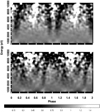 |
Fig. 1. Top: phase-energy diagram for the EPIC PN data of observation A, obtained by binning the source counts into energy and rotational phase channels, then normalizing to the phase-averaged energy spectrum and energy-integrated pulse profile. Bottom: same for observation B, when the source was in outburst. |
2. Data reduction
We compare our observation C with the two deepest archival observations (A and B, see Woods et al. 2004 for details on these observations). Observation A (2002-06-11) had a duration of 52 ks, with a net exposure time for the EPIC1 PN camera of 24.9 ks. Observation B (2002-06-21) had a duration of 31 ks, with a net exposure time for the EPIC PN camera of 18.5 ks. Observation B was performed while the source was in outburst, at a flux level that was about three times higher than the quiescent flux. Observation C (2014-07-29) had a duration of 112 ks, with a net exposure time for the EPIC PN camera of 100 ks.
We focused on the EPIC data from the PN instrument because of its higher time resolution (5.7 ms, Small Window mode, whereas the MOS cameras in Small Window mode have a time resolution of 0.3 s). In order to characterize possible phase-dependent features also in the low-energy region, we selected the 0.3−12.0 keV energy band, which is broader than the energy range commonly adopted in this type of studies (e.g., Zhu et al. 2008). The source extraction region is a circle with a radius of 40″. For the background, we chose two rectangular regions (90″ × 90″ and 90″ × 60″) at the border of the ∼4′ ×4′ PN Small Window, in order to minimize the contribution from the point spread function (PSF) of the central source.
3. Timing analysis
From the EPIC PN data set of observation C we generated a barycentered event file using the barycenter SAS tool. From the barycentered time series, we calculated the rotation period with a folding analysis (P = 6.979164(1) s). We also performed phase-connection analysis. The two values are consistent within 1σ. The uncertainties were evaluated through Monte Carlo simulations. With this value for the rotation period, we calculated the phase for the barycentered events with the phasecalc tool. We produced a phase-energy image for the EPIC PN observation by binning the source counts into energy and rotational phase channels (phase bin width: 0.02; energy bin width: 200 eV). This image was then normalized to the phase-averaged energy spectrum and the energy-integrated pulse profile. The visual inspection of such a phase-energy diagram (Fig. 2) shows a possible phase-dependent structure, as suggested (with a poorer counting statistics) by the archival observation A, namely a V-shaped feature spanning the plotted energy range. The data reduction and the creation of the phase-energy images performed on the X-ray data of observation C were also applied to the archival observations of 1E 2259+586 (A and B, Fig. 1).
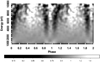 |
Fig. 2. Phase-energy diagram for the EPIC PN data of observation C, normalized as in Fig. 1. The V-shaped absorption profile is visible between phase 0.8 and 1.2. |
4. Spectral analysis
We generated the spectrum of observation C for the PN, and also for the two MOS, as a cross-check. We performed both a phase-averaged and a phase-resolved spectral analysis by dividing the observation into phase bins and fitting different spectral models in the XSPEC (Arnaud 1996) spectral analysis package. We compared the spectrum of observation C with the archival observations A and B.
4.1. Phase-averaged spectroscopy
In the XSPEC spectral analysis package, we adopted a phenomenological model made by a power-law and a blackbody component, modified by photoelectric absorption (TBabs*(pegpwrlw + bbodyrad)). When we fit this model to the phase-averaged PN spectrum of observation C, no acceptable fit was obtained (null hypothesis probability ∼10−10). A good fit was instead obtained by including a Gaussian absorption component (gabs). The best fit (χ2 = 1203.3 for 1157 degrees of freedom, null hypothesis probability = 0.18) is obtained for a broad (σ ≃ 3 keV) absorption line centered at ∼0.7 keV. The results of the best fit are reported in Table 2 and Fig. 5. Owing to the large number of counts in each spectral bin, systematic errors may be more relevant than the statistical errors. We therefore tested the possibility that this absorption feature was consistent with the systematic uncertainties. We plotted the residuals of the best fit obtained without the gabs component in units of data/model ratio. In the energy range around ∼0.7 keV, the residuals are about 10% or higher, which is far higher than the dynamical range of systematic uncertainties observed in EPIC-PN spectra (≲4%, see, e.g., Read et al. 2014 and references therein). This means that the observed absorption feature cannot be explained in terms of an incorrect calibration of the spectral response.
Best-fit model parameters (errors at 1σ confidence level) for the phase-averaged spectrum and the spectra of the four phase bins.
We analyzed the data from the two MOS cameras as well by fitting the spectral model adopted for the PN to the two MOS spectra simultaneously. A broad Gaussian absorption line at low energy is required here as well to obtain a satisfactory fit (χ2 = 2083.51, 1949 d.o.f., null hypothesis probability = 1.7 × 10⁻²; without line: χ2 = 2696.19; 1951 d.o.f., null hypothesis probability = ∼10−27, Fig. 6). The best-fit values for the parameters of the Gaussian absorption feature (gabs LineE = 0.87 ± 0.02 keV, gabs Sigma = 0.20 ± 0.01 keV) and some other parameters from the MOS are slightly different from those of the PN. A simultaneous fit to the MOS and PN spectra, leaving only a normalization factor for the different cameras free to vary, is not acceptable. Nonetheless, compatibility was obtained by considering a systematic error of ∼1.5−2% in the model parameters, which is within the range of the cross-calibration uncertainties between the three EPIC cameras (e.g., Read et al. 2014). A similar broad absorption feature at E ≃ 0.65 keV is also evident in the low-energy spectrum of observation A, but not in observation B, when 1E 2259+586 was much brighter and displayed a different continuum spectrum.
4.2. Phase-resolved spectroscopy
To characterize the high-energy phase-dependent spectral features identified through visual inspection of the phase-energy diagram, we first followed the procedure adopted by Tiengo et al. (2013) to detect the possible signature of a narrow phase-dependent cyclotron absorption line. Taking advantage of the high counting statistics, we divided the source PN event list of observation C into 50 phase bins of equal width (0.02). We fit the model for the entire observation (gabs*TBabs*(pegpwrlw + bbodyrad)) to the spectrum in each phase bin, with all parameters frozen to their best-fit value, including a free multiplicative factor (const) to account for different count rates in different bins. The spectra of the phase bins that are associated with the V-shaped dark feature that is apparent in the phase-energy image were inconsistent with the continuum emission model. The spectrum of one of the phase bins where a poor fit (null hypothesis probability < 0.003) was obtained is shown in Fig. 4. We therefore tried to fit the same model plus a cyclotron absorption line (const*cyclabs*gabs*TBabs*(pegpwrlw + bbodyrad)). The best fit was obtained for a very broad absorption line at energies above 1 keV. However, as suggested by the residuals in the top panel in Fig. 4, a fit with equivalent quality can be obtained by substituting the cyclotron line component with a high-energy cutoff or by letting the parameters of the power-law component free to vary. This indicates that some kind of phase-dependent spectral variability is present, but it cannot be straightforwardly modeled with a narrow absorption feature as in the case of SGR 0418+5729 (Tiengo et al. 2013).
Because the phase-resolved spectroscopy described above did not provide conclusive results on the phase variability in the high-energy (≳5 keV) region, we decided to divide the observation into broader phase intervals to better highlight the spectral evolution in phase. The X-ray light curve of 1E 2259+586 shows a double peak (Fig. 3, upper panel). The phase-energy image (not normalized for the pulse profile) displayed in the lower panel of Fig. 3 shows that the apparent V-shaped feature is located within the absolute minimum of the pulsation profile. In the high-energy region (≳5 keV) three distinct phase regions can be distinguished: two with a relative depletion of events (bars of the V) and a central region with a relative excess of events. At lower energy, the low signal-to-noise ratio of the data prevents us from clearly observing the tip of the V that connects the two bars. We divided the observation into the four phase bins shown in Fig. 3, which according to our inspection of the pulse profile and residual of the continuum modeling maximize the spectral differences along the phase axis. These phase intervals correspond to the two maxima (0.05−0.32 plus 0.62−0.83, bin 1); the relative minimum of the pulsation (0.32−0.62, bin 2); the event-depleted bars of the V on the sides of the absolute minimum of the pulsation (0.83−0.88 plus 0.98−0.05, bin 3); and the phase region located in the trough of the V, corresponding to the absolute minimum (0.88−0.98, bin 4)2.
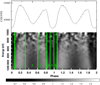 |
Fig. 3. Top: EPIC PN light curve in the energy range 0.3−12.0 keV for observation C. The double-peak pulse profile is clearly visible. Bottom: phase-energy diagram for the EPIC PN data obtained by binning the source counts into energy and rotational phase channels, then normalizing to the phase-averaged energy spectrum for the same observation (same as in Fig. 2, but not normalized to the energy-integrated pulse profile). The four phase bins used for the phase-resolved spectroscopy on the EPIC spectrum are identified by the green bars and numbers. |
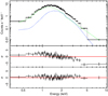 |
Fig. 4. Example of a spectral fit in one of the 50 phase bins we used for the phase-resolved spectroscopy. This is one of the bins located inside the bars of the V-shaped feature. Upper panel: results of the best fit for the const*cyclabs*gabs*TBabs*(pegpwrlw + bbodyrad) model (best-fit model for the phase-averaged spectrum plus a cyclotron absorption line) to the EPIC PN spectrum. The blackbody (blue line) and power-law (green line) components are plotted. Lower panels: residuals (in standard deviation units) for the best fit obtained without (χ2 = 539.2 for 347 d.o.f., null hypothesis probability ≃10−10), and with (χ2 = 360.2 for 344 d.o.f., null hypothesis probability = 0.26) the cyclotron absorption line. The best-fit parameters for the cyclotron absorption line are E = 1.0 keV and width W = 4.0 keV. A factor 5 graphic rebin is used. |
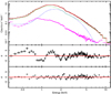 |
Fig. 5. Upper panel: results of the best fit for the EPIC PN phase-averaged spectrum of observation C (red line) obtained with a gabs*TBabs*(pegpwrlw + bbodyrad) model. The blackbody (blue line) and power-law (green line) components are plotted, as well as the spectrum of the background (magenta). Lower panels: residuals (in standard deviation units) for the best fit obtained without (top) and with (bottom) the gabs component. A factor 10 graphic rebin is used. |
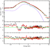 |
Fig. 6. Upper panel: results of the best fit for the EPIC MOS1 (black) and MOS2 (red) phase-averaged spectrum of observation C obtained with a gabs*TBabs*(pegpwrlw + bbodyrad) model. The blackbody (blue and magenta line) and power-law (green and yellow line) components are plotted. Lower panels: residuals (in standard deviation units) for the best fit obtained without (top) and with (bottom) the gabs component. A factor 10 graphic rebin is used. |
We simultaneously fit the phenomenological model used for the phase-averaged spectrum (gabs*TBabs (pegpwrlw+bbodyrad)) to the spectra of the four bins. We included a free overall normalization factor (const) to account for the different flux levels of the spectra in different bins. We linked the value of the parameters across the four bins, leaving only some of them free to vary from bin to bin. By leaving only the overall normalization (const) free to vary across the four bins, no acceptable fit is obtained (χ2 = 4127.1 for 3192 d.o.f., null-hypothesis probability ∼10−27). In the same way, linking the parameters of the power-law component and leaving the parameters of the blackbody component free to vary, no acceptable fit is obtained. On the other hand, by leaving the parameters of the power-law component free to vary independently (with linked blackbody parameters), we obtained a very good fit (χ2 = 3221.8 for 3128 d.o.f., null-hypothesis probability = 0.118). The spectra of the four bins together with the best-fit model are shown in Fig. 7, and the corresponding best-fit values for the photon index and normalization for the power-law component are reported in Table 2.
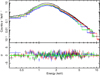 |
Fig. 7. Results of the joint fit for the four phase-resolved EPIC PN spectra of observation C. Black: Bin 1. Red: Bin 2. Green: Bin 3. Blue: Bin 4. Lower panel: residuals (in standard deviation units) for each spectrum. A factor 10 graphic rebin is used. |
For each of the four spectra, we computed a contour plot of the best-fit photon index against the power-law normalization (Fig. 8). The parameters of the blackbody component were the same for each bin. Because we kept the blackbody normalization constant across the four bins (which was made possible by introducing an overall normalization factor, const) the value of the power-law component normalization in each bin represents the relative flux of the power-law component with respect to the blackbody. This allowed us to evaluate the relative strength of the power-law and blackbody components in the spectrum. From the contour plot, it is evident that regardless of the overall normalization factor, all spectra are inconsistent with each other, except for bins 1 and 4.
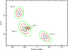 |
Fig. 8. Contour plots for the 1, 2, and 3σ contours of the values of photon index and normalization (unabsorbed flux in the 2−10 keV band in units of 10−12 erg s−1 cm−2 divided by the constant factors reported in Table 2) of the power-law component of the best-fit model (const*gabs*TBabs*(pegpwrlw+bbodyrad)) for the four phase bins used in the phase-resolved spectroscopy. |
Following Tiengo et al. (2013), we tested the addition of a cyclotron absorption line component to the phase-averaged model and fit it to the spectra of the four bins, leaving only the parameters of the line free to vary across different bins, and linking all the others. As for the spectra of some of the narrow phase intervals, the addition of a (broad) cyclotron absorption line to the model was sufficient to obtain an acceptable fit also for all the spectra of the four broad phase intervals. The results we obtained are comparable in terms of the goodness of fit to what we obtained by leaving the parameters of the power-law component free to vary in the simpler continuum model we adopted for the phase-averaged spectrum. There is therefore no statistical evidence that a cyclotron absorption line is needed to describe the phase variability observed in the phase-energy diagram of 1E 2259 + 586.
As shown by Fernández & Thompson (2007) and Nobili et al. (2008), spectra produced by resonant Compton scattering (RCS) of thermal photons by magnetospheric currents show a distinct phase-dependence that affects the power-law tail at energies above ∼5 keV. Motivated by this, we performed a fit to the phase-averaged spectrum with the RCS model (ntznoang in XSPEC; Nobili et al. 2008; Zane et al. 2009). The best fit ( for 1183 d.o.f.) yields T = 0.38 keV, βbulk = 0.20, Δϕ = 0.86 rad and an overall normalization factor of 0.56 for the model parameters (here T, βbulk, and Δϕ are the surface temperature, the bulk electron velocity in units of c, and the twist angle, respectively; see Nobili et al. 2008 for more details). We computed the phase-resolved spectra for the model parameters obtained from the fit of the phase-averaged spectrum, and a few combinations of χ and ξ, the two angles that the star rotation axis makes with the line of sight and the dipole axis. While the phase-averaged spectrum is quite insensitive to the source geometry, phase-resolved spectra depend on χ and ξ, so that different choices of χ and ξ yield different phase-dependent variability in the continuum spectrum. Results confirm that the observed spectral variations with phase can indeed be recovered within the RCS model for suitable geometries.
We considered the possibility that also the 0.7 keV feature discovered in the phase-averaged spectrum shows a phase dependence. The distribution of residuals in both the 50-bin and 4-bin analysis does not provide any evidence of phase variability for the 0.7 keV feature. Nonetheless, Fig. 2 shows possible structures in the E < 1 keV region: an apparent depletion of events at phase ∼0.2 and ∼0.8. However, also when we divided the observation into two phase bins (0.12−0.24 plus 0.74−0.82 and 0.24−0.74 plus 0.82−0.12) and fit the phase-averaged model to their spectra, leaving the gabs energy free to vary, we did not find significant variability.
5. Discussion
Absorption features in the X-ray spectra of neutron stars are considered an astrophysical “holy grail” because by comparing the observed and intrinsic energy of lines of unambiguous origin, the gravitational redshift can be measured. This depends on the neutron star compactness (M/R), which would allow placing constraints on the equation of state (EOS) of nuclear matter. Furthermore, understanding the physical origin of spectral features is fundamental for determining the composition of a possible atmosphere and thus fit the thermal emission spectra with the most appropriate models. Broad absorption features centered at some hundreds of eV have repeatedly been observed in the spectra of most X-ray dim isolated neutron stars (XDINSs), as single or harmonically spaced features, which often display spectral phase variability (Haberl et al. 2003, 2004; van Kerkwijk et al. 2004; Zane et al. 2005; Schwope et al. 2007; Haberl 2007; Borghese et al. 2015, 2017). XDINSs are a class of radio-quiet isolated neutron stars that are characterized by purely thermal X-ray spectra. The apparent lack of contamination from nonthermal magnetospheric emission in their spectra makes these stars very good candidates for spectral studies that are aimed at constraining the EOS. Phase-dependent harmonically spaced absorption lines were revealed in the radio-quiet pulsar 1E 1207.4-5209 (fundamental at 0.7 keV, plus two or possibly three harmonics, Sanwal et al. 2002; Mereghetti et al. 2002; Bignami et al. 2003, De Luca et al. 2004), as well as in the rotating radio transient PSR J1819−1458 (at ∼0.5 keV and ∼1 keV, McLaughlin et al. 2007). More recently, absorption lines have also been found in standard rotation-powered radio pulsars (e.g., PSR J1740+1000, Kargaltsev et al. 2012; PSR B0628–28, Rigoselli & Mereghetti 2018, PSR J0656+1414, Arumugasamy et al. 2018).
In order to obtain a good fit for the high statistics spectrum of 1E 2259+586 provided by our deep EPIC exposure, we had to introduce a broad Gaussian absorption line (σ ∼ 0.3 keV) at ∼0.7 keV. This line was detected with high significance in the phase-averaged spectrum. The properties of this broad feature are similar to those of the lines detected in some XDINS, and when we interpret it as a cyclotron line, it implies a magnetic field of 6 × 10¹⁰ (1+z) G or 1.1 × 10¹⁴ (1+z) G in the case of electrons or protons, respectively. This is to be compared with the dipole field of ∼6 × 10¹³ G derived from the timing parameters of 1E 2259+586. Using a typical value for the neutron star M/R (0.12 M⊙/km, Sammarruca & Millerson 2019) and the following gravitational redshift (z = 0.25), we obtain a value in the proton scattering scenario that is consistent, within an order of magnitude with the magnetic field inferred from timing. The large width and the lack of variability of this line throughout the magnetar rotation are consistent with proton cyclotron scattering in the global magnetic field close to the surface of the neutron star. In particular, following Zane et al. (2001), we derive an expected line width of ∼0.35 keV, which is in very good agreement with our best-fit value of 0.33 keV. However, given the apparent absence of phase variability of this feature, we cannot completely rule out the possibility of a spurious origin that is due to calibration issue. On the other hand, the detection of this absorption feature in the EPIC MOS spectra as well, although with slightly different best-fit parameters, suggests that it is not a calibration artifact. Another possibility is that the feature we found in 1E 2259+586 is due to an inadequate modeling of the interstellar absorption in our spectra.
Our long observation of 1E 2259+586 was primarily motivated by the features observed in the phase-energy images derived from previous XMM-Newton observations of this source (see Fig. 1 and Fig. 2). They resemble those found in the transient magnetars SGR 0418+5729 and SWIFT J1822.3−1606, which were interpreted as proton cyclotron lines in localized regions of strong magnetic field (Tiengo et al. 2013; Rodríguez Castillo et al. 2016). The phase-energy images displayed in Figs. 1 and 2 are quite similar to those of SGR 0418+5729 and SWIFT J1822.3−1606. In particular, the behavior of 1E 2259+586 in outburst (observation B, bottom panel of Fig. 1), with the single slightly inclined dark feature discovered in the present work (at phase ∼0.8) resembles that of SWIFT J1822.3−1606, whereas the V-shaped dark feature that appears during the quiescent observations (A, C) recalls the feature that was observed in SGR 0418+5729. However, the V-shaped feature in our observation C looks somewhat different from the feature observed in SGR 0418+5729 because its relative strength is lower, especially at the lowest energies, and it appears less extended in rotational phase.
If a proton cyclotron interpretation were acceptable, then this variation would suggest a different geometry of the strong multipolar magnetic field components and/or of the hot regions that generate the photons that interact with the magnetospheric protons between the quiescence and outburst phase. However, the spectral variability of 1E 2259+586 cannot be straightforwardly modeled with a proton cyclotron model as in the basic model proposed for SGR 0418+5729 (Tiengo et al. 2013). We therefore described the high-quality phase-resolved spectrum obtained from our observation C with a phenomenological model, where the bulk of the X-ray emission is provided by the sum of a blackbody and a power-law component. In this context, the spectral changes of 1E 2259+586 along its pulsation phase can be fully attributed to a phase-dependence of the power-law slope and of its intensity with respect to that of the blackbody component. The results of the fit of the ntzang model to the spectra of the four broad phase bins suggest that the phase variability in the continuum of the spectrum of observation C is indeed consistent with RCS in the magnetosphere. It is interesting to note that despite their significantly different flux, the spectral shapes of the two maxima and of the absolute minimum are consistent with each other. On the other hand, the hardest and softest spectra are observed in the secondary minimum and in two narrow-phase intervals around the absolute minimum.
6. Conclusions
We have carried out a long XMM-Newton observation of the persistent magnetar 1E 2259+586, with the main objective to search for phase-dependent spectral features. We found that the phase-averaged spectrum is well fit by a phenomenological model consisting of the combination of an absorbed blackbody plus power law with a Gaussian absorption line (E ∼ 0.7 keV) accounting for a phase-independent deficit of counts at low energies. This broad (∼0.3 keV) absorption feature resembles the features that are detected in the X-ray spectra of other isolated neutron stars, and in particular, in most XDINSs. If this line is caused by proton cyclotron resonant scattering, the inferred magnetic field is not much different from that derived from pulsar spin-down parameters. On the other hand, if it is due to electrons, the derived field is more than two orders of magnitude smaller than the surface dipole field, implying an origin high in the stellar magnetosphere.
We found that the spectrum of 1E 2259+586 varies significantly as a function of the rotational phase, especially at energies > 2 keV. Although the phase-energy images of 1E 2259+586 in quiescence and in outburst resemble those of the low field magnetars SGR 0418+5729 and SWIFT J1822.3-1606, respectively, in this case, the phase-resolved X-ray spectra cannot be fit by a simple model with a narrow phase-variable cyclotron absorption feature. We found instead that the phase-dependent spectral variations can be entirely explained in terms of changes in the continuum emission, namely a significant variation (> 3σ) in the hardness and normalization of the power-law spectral component. We suggest that this variability can be attributed to RCS in the twisted global dipole field of the magnetar.
The European Photon Imaging Camera (EPIC) is located at the focus of the three grazing-incidence multi-mirror X-ray telescopes that constitute the main instrument of XMM-Newton; it consists of three CCD cameras: one PN and two MOS (Strüder et al. 2001, Turner et al. 2001).
Acknowledgments
This work is based on observations obtained with XMM-Newton, an ESA science mission with instruments and contributions directly funded by ESA Member States and NASA. PE acknowledges funding in the framework of the project ULTraS, ASI–INAF contract N. 2017-14-H.0. LS acknowledges financial contributions from ASI-INAF agreements 2017-14-H.O and I/037/12/0 and from iPeska research grant (P.I. Andrea Possenti) funded under the INAF call PRIN-SKA/CTA (resolution 70/2016). FCZ is supported by grant AYA2015-71042-P.
References
- Arnaud, K. A. 1996, in Astronomical Data Analysis Software and Systems V, eds. G. H. Jacoby, & J. Barnes, ASP Conf. Ser., 101, 17 [NASA ADS] [Google Scholar]
- Arumugasamy, P., Kargaltsev, O., Posselt, B., Pavlov, G. G., & Hare, J. 2018, ApJ, 869, 97 [NASA ADS] [CrossRef] [Google Scholar]
- Bignami, G. F., Caraveo, P. A., De Luca, A., & Mereghetti, S. 2003, Nature, 423, 725 [NASA ADS] [CrossRef] [PubMed] [Google Scholar]
- Borghese, A., Rea, N., Coti Zelati, F., Tiengo, A., & Turolla, R. 2015, ApJ, 807, L20 [NASA ADS] [CrossRef] [Google Scholar]
- Borghese, A., Rea, N., Coti Zelati, F., et al. 2017, MNRAS, 468, 2975 [NASA ADS] [CrossRef] [Google Scholar]
- De Luca, A., Mereghetti, S., Caraveo, P. A., et al. 2004, A&A, 418, 625 [NASA ADS] [CrossRef] [EDP Sciences] [Google Scholar]
- Dib, R., & Kaspi, V. M. 2014, ApJ, 784, 37 [NASA ADS] [CrossRef] [Google Scholar]
- Duncan, R. C., & Thompson, C. 1992, ApJ, 392, L9 [NASA ADS] [CrossRef] [Google Scholar]
- Fahlman, G. G., & Gregory, P. C. 1981, Nature, 293, 202 [NASA ADS] [CrossRef] [Google Scholar]
- Fahlman, G. G., & Gregory, P. C. 1983, in Supernova Remnants and their X-ray Emission, eds. J. Danziger, & P. Gorenstein, IAU Symp., 101, 445 [NASA ADS] [CrossRef] [Google Scholar]
- Fernández, R., & Thompson, C. 2007, ApJ, 660, 615 [NASA ADS] [CrossRef] [Google Scholar]
- Haberl, F. 2007, Ap&SS, 308, 181 [NASA ADS] [CrossRef] [Google Scholar]
- Haberl, F., Schwope, A. D., Hambaryan, V., Hasinger, G., & Motch, C. 2003, A&A, 403, L19 [NASA ADS] [CrossRef] [EDP Sciences] [Google Scholar]
- Haberl, F., Motch, C., Zavlin, V. E., et al. 2004, A&A, 424, 635 [NASA ADS] [CrossRef] [EDP Sciences] [Google Scholar]
- Kargaltsev, O., Durant, M., Misanovic, Z., & Pavlov, G. G. 2012, Science, 337, 946 [NASA ADS] [CrossRef] [Google Scholar]
- Kaspi, V. M., & Beloborodov, A. M. 2017, ARA&A, 55, 261 [NASA ADS] [CrossRef] [Google Scholar]
- Kaspi, V. M., Gavriil, F. P., Woods, P. M., et al. 2003, ApJ, 588, L93 [NASA ADS] [CrossRef] [Google Scholar]
- Kothes, R., & Foster, T. 2012, ApJ, 746, L4 [NASA ADS] [CrossRef] [Google Scholar]
- Livingstone, M. A., Ng, C.-Y., Kaspi, V. M., Gavriil, F. P., & Gotthelf, E. V. 2011, ApJ, 730, 66 [NASA ADS] [CrossRef] [Google Scholar]
- McLaughlin, M. A., Rea, N., Gaensler, B. M., et al. 2007, ApJ, 670, 1307 [NASA ADS] [CrossRef] [Google Scholar]
- Mereghetti, S., De Luca, A., Caraveo, P. A., et al. 2002, ApJ, 581, 1280 [NASA ADS] [CrossRef] [Google Scholar]
- Mereghetti, S., Pons, J. A., & Melatos, A. 2015, Space Sci. Rev., 191, 315 [NASA ADS] [CrossRef] [Google Scholar]
- Nobili, L., Turolla, R., & Zane, S. 2008, MNRAS, 386, 1527 [NASA ADS] [CrossRef] [Google Scholar]
- Paczynski, B. 1992, Acta Astron., 42, 145 [NASA ADS] [Google Scholar]
- Rea, N., Esposito, P., Turolla, R., et al. 2010, Science, 330, 944 [NASA ADS] [CrossRef] [PubMed] [Google Scholar]
- Rea, N., Israel, G. L., Esposito, P., et al. 2012, ApJ, 754, 27 [NASA ADS] [CrossRef] [Google Scholar]
- Rea, N., Israel, G. L., Pons, J. A., et al. 2013, ApJ, 770, 65 [NASA ADS] [CrossRef] [Google Scholar]
- Read, A. M., Guainazzi, M., & Sembay, S. 2014, A&A, 564, A75 [NASA ADS] [CrossRef] [EDP Sciences] [Google Scholar]
- Rigoselli, M., & Mereghetti, S. 2018, A&A, 615, A73 [NASA ADS] [CrossRef] [EDP Sciences] [Google Scholar]
- Rodríguez Castillo, G. A., Israel, G. L., Tiengo, A., et al. 2016, MNRAS, 456, 4145 [NASA ADS] [CrossRef] [Google Scholar]
- Sammarruca, F., & Millerson, R. 2019, J. Phys. G Nucl. Phys., 46, 024001 [NASA ADS] [CrossRef] [Google Scholar]
- Sanwal, D., Pavlov, G. G., Zavlin, V. E., & Teter, M. A. 2002, ApJ, 574, L61 [NASA ADS] [CrossRef] [Google Scholar]
- Schwope, A. D., Hambaryan, V., Haberl, F., & Motch, C. 2007, Ap&SS, 308, 619 [NASA ADS] [CrossRef] [Google Scholar]
- Strüder, L., Briel, U., Dennerl, K., et al. 2001, A&A, 365, L18 [NASA ADS] [CrossRef] [EDP Sciences] [Google Scholar]
- Thompson, C., & Duncan, R. C. 1995, MNRAS, 275, 255 [NASA ADS] [CrossRef] [Google Scholar]
- Thompson, C., & Duncan, R. C. 1996, ApJ, 473, 322 [NASA ADS] [CrossRef] [Google Scholar]
- Thompson, C., Lyutikov, M., & Kulkarni, S. R. 2002, ApJ, 574, 332 [NASA ADS] [CrossRef] [Google Scholar]
- Tiengo, A., Esposito, P., Mereghetti, S., et al. 2013, Nature, 500, 312 [NASA ADS] [CrossRef] [PubMed] [Google Scholar]
- Turner, M. J. L., Abbey, A., Arnaud, M., et al. 2001, A&A, 365, L27 [NASA ADS] [CrossRef] [EDP Sciences] [Google Scholar]
- Turolla, R., Zane, S., & Watts, A. L. 2015, Rep. Prog. Phys., 78, 116901 [Google Scholar]
- van Kerkwijk, M. H., Kaplan, D. L., Durant, M., Kulkarni, S. R., & Paerels, F. 2004, ApJ, 608, 432 [NASA ADS] [CrossRef] [Google Scholar]
- Woods, P. M., Kaspi, V. M., Thompson, C., et al. 2004, ApJ, 605, 378 [NASA ADS] [CrossRef] [Google Scholar]
- Zane, S., Turolla, R., Stella, L., & Treves, A. 2001, ApJ, 560, 384 [NASA ADS] [CrossRef] [Google Scholar]
- Zane, S., Cropper, M., Turolla, R., et al. 2005, ApJ, 627, 397 [NASA ADS] [CrossRef] [Google Scholar]
- Zane, S., Rea, N., Turolla, R., & Nobili, L. 2009, MNRAS, 398, 1403 [NASA ADS] [CrossRef] [Google Scholar]
- Zhu, W., Kaspi, V. M., Dib, R., et al. 2008, ApJ, 686, 520 [NASA ADS] [CrossRef] [Google Scholar]
All Tables
Best-fit model parameters (errors at 1σ confidence level) for the phase-averaged spectrum and the spectra of the four phase bins.
All Figures
|
Fig. 1. Top: phase-energy diagram for the EPIC PN data of observation A, obtained by binning the source counts into energy and rotational phase channels, then normalizing to the phase-averaged energy spectrum and energy-integrated pulse profile. Bottom: same for observation B, when the source was in outburst. |
| In the text | |
|
Fig. 2. Phase-energy diagram for the EPIC PN data of observation C, normalized as in Fig. 1. The V-shaped absorption profile is visible between phase 0.8 and 1.2. |
| In the text | |
|
Fig. 3. Top: EPIC PN light curve in the energy range 0.3−12.0 keV for observation C. The double-peak pulse profile is clearly visible. Bottom: phase-energy diagram for the EPIC PN data obtained by binning the source counts into energy and rotational phase channels, then normalizing to the phase-averaged energy spectrum for the same observation (same as in Fig. 2, but not normalized to the energy-integrated pulse profile). The four phase bins used for the phase-resolved spectroscopy on the EPIC spectrum are identified by the green bars and numbers. |
| In the text | |
|
Fig. 4. Example of a spectral fit in one of the 50 phase bins we used for the phase-resolved spectroscopy. This is one of the bins located inside the bars of the V-shaped feature. Upper panel: results of the best fit for the const*cyclabs*gabs*TBabs*(pegpwrlw + bbodyrad) model (best-fit model for the phase-averaged spectrum plus a cyclotron absorption line) to the EPIC PN spectrum. The blackbody (blue line) and power-law (green line) components are plotted. Lower panels: residuals (in standard deviation units) for the best fit obtained without (χ2 = 539.2 for 347 d.o.f., null hypothesis probability ≃10−10), and with (χ2 = 360.2 for 344 d.o.f., null hypothesis probability = 0.26) the cyclotron absorption line. The best-fit parameters for the cyclotron absorption line are E = 1.0 keV and width W = 4.0 keV. A factor 5 graphic rebin is used. |
| In the text | |
|
Fig. 5. Upper panel: results of the best fit for the EPIC PN phase-averaged spectrum of observation C (red line) obtained with a gabs*TBabs*(pegpwrlw + bbodyrad) model. The blackbody (blue line) and power-law (green line) components are plotted, as well as the spectrum of the background (magenta). Lower panels: residuals (in standard deviation units) for the best fit obtained without (top) and with (bottom) the gabs component. A factor 10 graphic rebin is used. |
| In the text | |
|
Fig. 6. Upper panel: results of the best fit for the EPIC MOS1 (black) and MOS2 (red) phase-averaged spectrum of observation C obtained with a gabs*TBabs*(pegpwrlw + bbodyrad) model. The blackbody (blue and magenta line) and power-law (green and yellow line) components are plotted. Lower panels: residuals (in standard deviation units) for the best fit obtained without (top) and with (bottom) the gabs component. A factor 10 graphic rebin is used. |
| In the text | |
|
Fig. 7. Results of the joint fit for the four phase-resolved EPIC PN spectra of observation C. Black: Bin 1. Red: Bin 2. Green: Bin 3. Blue: Bin 4. Lower panel: residuals (in standard deviation units) for each spectrum. A factor 10 graphic rebin is used. |
| In the text | |
|
Fig. 8. Contour plots for the 1, 2, and 3σ contours of the values of photon index and normalization (unabsorbed flux in the 2−10 keV band in units of 10−12 erg s−1 cm−2 divided by the constant factors reported in Table 2) of the power-law component of the best-fit model (const*gabs*TBabs*(pegpwrlw+bbodyrad)) for the four phase bins used in the phase-resolved spectroscopy. |
| In the text | |
Current usage metrics show cumulative count of Article Views (full-text article views including HTML views, PDF and ePub downloads, according to the available data) and Abstracts Views on Vision4Press platform.
Data correspond to usage on the plateform after 2015. The current usage metrics is available 48-96 hours after online publication and is updated daily on week days.
Initial download of the metrics may take a while.