| Issue |
A&A
Volume 700, August 2025
|
|
|---|---|---|
| Article Number | A19 | |
| Number of page(s) | 10 | |
| Section | Stellar structure and evolution | |
| DOI | https://doi.org/10.1051/0004-6361/202554386 | |
| Published online | 25 July 2025 | |
The Northern Cross Fast Radio Burst project
V. Search for transient radio emission from Galactic magnetars
1
Scuola Universitaria Superiore IUSS Pavia, Palazzo del Broletto, Piazza della Vittoria 15, I-27100 Pavia, Italy
2
Dipartimento di Fisica, Università di Trento, Via Sommarive 14, I-38123 Povo, (TN), Italy
3
INAF–Osservatorio Astronomico di Cagliari, Via della Scienza 5, I-09047 Selargius, (CA), Italy
4
INAF–Istituto di Astrofisica Spaziale e Fisica Cosmica di Milano, Via Corti 12, I-20133 Milano, Italy
5
INAF–Istituto di Radio Astronomia (IRA), Via Piero Gobetti 101, I-40129 Bologna, Italy
6
South African Radio Astronomy Observatory, Black River Park, 2 Fir Street, Observatory, Cape Town 7925, South Africa
7
Department of Physics and Electronics, Rhodes University, PO Box 94 Makhanda 6140, South Africa
8
Dipartimento di Fisica e Astronomia, Università di Bologna, Via Gobetti 93/2, I-40129 Bologna, Italy
9
Dipartimento di Fisica e Astronomia, Università di Padova, Via Marzolo 8, I-35131 Padova, Italy
10
Mullard Space Science Laboratory, University College London, Holmbury St Mary, Dorking, Surrey RH5 6NT, UK
11
INAF–Osservatorio Astronomico di Roma, Via Frascati 33, I-00078 Monteporzio Catone, Italy
12
ASI–Space Science Data Center, Via del Politecnico snc, I-00133 Roma, (RM), Italy
13
INAF–IAPS, Via del Fosso del Cavaliere 100, I-00133 Roma, (RM), Italy
14
INFN Tor Vergata, Via della Ricerca Scientifica, I-00133 Roma, (RM), Italy
15
Institute of Space Sciences and Astronomy (ISSA), University of Malta, Msida MSD 2080, Malta
16
Dipartimento di Fisica, Università degli Studi di Roma “Tor Vergata”, Via della Ricerca Scientifica 1, I-00133 Roma, (RM), Italy
⋆ Corresponding author: andrea.geminardi@iusspavia.it
Received:
5
March
2025
Accepted:
29
May
2025
Context. The radio emission from magnetars is poorly understood and poorly characterized observationally, particularly for what concerns single pulses and sporadic events. Interest in this type of radio emission has been boosted by the detection of an extremely bright millisecond radio signal from the Galactic magnetar designated as SGR J1935+2154 in 2020, which occurred almost simultaneously with a typical magnetar short burst of X-rays. As of now, this event remains the Galactic radio pulse that is the most reminiscent of fast radio bursts, and it is the only one that has a sound association with a known progenitor.
Aims. We aim to constrain the rate of impulsive radio events from magnetars by means of intensive monitoring using a high-sensitivity radio telescope.
Methods. We performed a long-term campaign on seven Galactic magnetars (plus one candidate) using the Northern Cross transit radio telescope (in Medicina, Italy), searching for short timescales and dispersed radio pulses.
Results. We obtained no detections in ∼560 hours of observation, setting an upper limit at a 95% confidence level of < 52 yr−1 on the rate of events with energy ≳1028 erg, which is consistent with limits in the literature. Furthermore, under some assumptions regarding the properties and energetic behavior of magnetars, we find that our upper limits point toward the fact that the entire population of observed fast radio bursts cannot be explained by radio bursts emitted by magnetars.
Key words: stars: magnetars / pulsars: general
© The Authors 2025
 Open Access article, published by EDP Sciences, under the terms of the Creative Commons Attribution License (https://creativecommons.org/licenses/by/4.0), which permits unrestricted use, distribution, and reproduction in any medium, provided the original work is properly cited.
This article is published in open access under the Subscribe to Open model. Subscribe to A&A to support open access publication.
1. Introduction
Magnetars are a class of neutron stars characterized by their high magnetic field strength (1014 − 1015 G) and their peculiar emission behavior (Mereghetti 2008; Turolla et al. 2015; Kaspi & Beloborodov 2017; Esposito et al. 2021). These compact objects can exhibit persistent and transient X-ray emission and, in some cases, also optical and infrared counterparts (Chrimes et al. 2025 and references therein). The signature feature of magnetars is their bursting activity. In addition, their emission and timing properties can undergo enormous changes over different timescales, and these sharp variations are unpredictable (Rea & Esposito 2011). The longest magnetar events are the outburst phases, where the X-ray luminosity grows by a few orders of magnitude with respect to the quiescent phases, and they can last from weeks to years (Coti Zelati et al. 2018). On shorter timescales, magnetars exhibit explosive events such as short bursts (≲1 s and luminosity L ≈ 1036 − 1043 erg s−1), which are often clustered in activity windows that can last for days (Göǧüş et al. 2001; Israel et al. 2008; Esposito et al. 2008). The rarest events at shorter timescales are extremely energetic giant flares, during which the initial millisecond gamma-ray flash (L ≈ 1045 − 1047 erg s−1) is followed by a fading X-ray and γ-ray afterglow modulated at the neutron star spin period that can last for minutes and has a characteristic total energy of ≈1044 erg (Mazets et al. 1979a; Hurley et al. 1999a; Palmer et al. 2005). So far, the number of Galactic sources identified as magnetars is around 30 (Olausen & Kaspi 2014)1. However, the number of these sources in our Galaxy is expected to be much higher (Muno et al. 2008; Gullón et al. 2015; Pardo et al., in prep.). At radio wavelengths, ephemeral pulsations have been detected only from five magnetars during outburst phases (Camilo et al. 2006, 2007; Levin et al. 2010; Rea et al. 2013a; Esposito et al. 2020, and references therein)2. The energy involved in their radio emission is comparable or higher with respect to standard rotation-powered pulsars, while some clearly different features distinguish the bursting behaviors of these two classes (Kramer et al. 2007). Radio pulses coming from magnetars present a harder spectrum (∝ν−0.5). In particular, the short timescale and unpredictable variations of the shapes of the pulses do not permit identification of a characteristic pulsing profile.
Owing to their extreme properties and bursting behavior, magnetars are often invoked in various astrophysical phenomena, such as gamma-ray bursts or super-luminous supernovae engines and ultra-luminous X-ray sources (Dall’Osso & Stella 2022). In recent years, one of the most intriguing proposed magnetar associations is that with the so-called fast radio bursts (FRBs Popov et al. 2018; Bailes 2022; Zhang 2023).
Fast radio bursts are powerful millisecond bursts of celestial origin detected only at radio frequencies. Their highspectral luminosity, typically greater than 1030 erg s−1 Hz−1, and extreme brightness temperature (≳1030 K, with some of them exceeding 1036 K) suggest coherent emission mechanisms in compact sources (Nimmo et al. 2022). Among the great variety of models proposed to explain these intriguing signals, those involving the magnetosphere of magnetars or shocks beyond the magnetosphere are among the most popular and promising (Platts et al. 2019). Since their discovery in 2007 (Lorimer et al. 2007), more than 800 FRB sources have been found (Xu et al. 2023), and current estimations suggest a high all-sky rate of FRBs of ∼500 per day above a 5 Jy ms threshold at 600 MHz (CHIME/FRB Collaboration 2023a). Fast radio bursts show high flux densities (a few Jy, approximately reaching the kJy level in a few cases; CHIME/FRB Collaboration 2024), and their characteristic high dispersion measure (DM), which far exceeds the predicted Galactic contribution in the directions of arrival of the FRBs, points to an extragalactic origin. Some associations with galaxies, with the most distant detected so far at redshift z ∼ 1 (Ryder et al. 2023), suggest that FRBs can come from great distances and could be exploited in cosmological studies (Gupta et al. 2025).
The main subdivision in the FRB population is between sources detected only once (one-off FRBs) and those that have shown recurrent activity (FRB repeaters), which comprise ∼8% of the known population (Xu et al. 2023)3. Current knowledge and understanding of FRBs is not sufficient to assess whether the repeating sources represent a standalone population with respect to one-off FRBs and not even whether they are produced by the same sources or mechanisms (Pleunis et al. 2021). Today, despite many efforts, there are no counterparts associated with any known extragalactic FRBs.
The suggested link between magnetars and FRBs was strengthened by the peculiar radio activity observed from SGR J1935+2154, which was an “ordinary” magnetar up until that point. In 2020, this source emitted several bright millisecond radio bursts (CHIME/FRB Collaboration 2020; Bochenek et al. 2020; Kirsten et al. 2021; Rehan & Ibrahim 2025). One of these was extremely bright (CHIME/FRB Collaboration 2020), lasted for ∼1 ms, and reached a fluence of 480 kJy ms at 400−800 MHz and a MJy ms fluence at 1.4 GHz. To date, this Galactic radio signal is the most reminiscent of FRBs, although the inferred energy released was a few orders of magnitude lower than the typical FRB energy.
In this work, we aim to constrain the radio-bursting activity of magnetar-like objects. We focused our search on millisecond-long transients coming from Galactic magnetars with intense monitoring at high sensitivity. Our campaign is sensitive to both FRB-like events and giant pulses coming from the observed magnetars (Lundgren et al. 1995; Camilo et al. 2006; Israel et al. 2021; Caleb et al. 2022). Furthermore, under some assumptions, we exploited our observations to investigate the magnetar energy spectrum and their high-energy behavior.
This paper is organized as follows: In Section 2 we describe the targets observed in this work. In Section 3, we outline how the data were stored and analyzed. Section 4 presents the model used to obtain the results that are listed and discussed in Section 5. Finally, in Section 6 we discuss the results and summarize our work.
2. Targets
In this section, we summarize the properties of the sample of magnetars that we observed. We monitored all the currently known Galactic magnetars that are visible from the Northern Cross (NC) site in Medicina, near Bologna, Italy (Olausen & Kaspi 2014). Most of the targets are located in the direction of the Galactic plane. Table 1 shows the coordinates and estimated DMs for each source. We performed DM estimations using the models of Cordes & Lazio (2002) and Yao et al. (2017) based on the electron density distribution in the Galaxy and using the best fit of the relation between the DM and the observed hydrogen column density ofHe et al. (2013).
Localization and predicted Galactic DM contributions for the magnetar sample.
2.1. 3XMM J185246.6+003317
In 2014, 3XMM J185246.6+003317 was discovered and identified as a magnetar (Zhou et al. 2014). Based on re-analysis of XMM-Newton data, this source was found to have had an outburst phase between 2008 and 2009. The neutron star rotates with a period of P ∼ 11.56 s, and the upper limit on the spin period derivative is Ṗ < 1.4 × 10⁻¹³ s s−1, implying adipolar surface magnetic field of Bdip < 4.1 × 10¹³ G (Rea et al. 2014). These are typical parameters of a low magnetic field (low-B) aged magnetar. No radio signals have ever been detected from this source. We note that 3XMM J185246.6+003317 is located at a distance of 1′ from the supernova remnant Kes 79, and the two objects have similar absorption properties. Therefore, as in Zhou et al. (2014), we assumed ∼7.1 kpc as the distance for both Kes 79 and the magnetar. The sky coordinates used for the observations of this target are RA = 18h52m46.67s, Dec = +00° 33′17.8″ (J2000).
2.2. SGR 1900+14
Discovered in 1979 (Mazets et al. 1979b), SGR 1900+14 is a persistent X-ray source. It has a spin period of P ∼ 5.20 s and a period derivative of Ṗ ∼ 9.2 × 10⁻¹¹ s s−1 (Mereghetti et al. 2006). The inferred surface magnetic field is Bdip ∼ 8 × 10¹⁴ G (Kouveliotou et al. 1999). SGR 1900+14 emitted a giant flare in 1998 (Hurley et al. 1999a), reaching a total energy of ∼1044 erg, and in the following years, several high-energy bursts were detected from this target. Based on observations from the Very Large Array (VLA), a fading radio source was associated with this object just after the giant flare (Frail et al. 1999). Similar to what was observed for SGR 1806−20 after its 2004 giant flare (Cameron et al. 2005), the radio source was tentatively attributed to an outflow of relativistic particles. The distance from Earth of this magnetar is not well established. Kouveliotou et al. (1999) and Hurley et al. (1999b) estimated a distance between 5 and 7 kpc, while others, such as Mereghetti et al. (2006) and Davies et al. (2009), locate the magnetar between 12.5 and 15 kpc. According to the kinematic distance estimated in Davies et al. (2009), we assumed a distance of 12.0 ± 1.7 kpc and the sky coordinates RA = 19h06m53.7s, Dec = +09° 20′47.0″ (J2000).
2.3. SGR J1935+2154
The source SGR J1935+2154 was identified as a magnetar in 2015 (Israel et al. 2016) without a detected radio counterpart. The pulsation period is P ∼ 3.24 s, and the spin-down rate is Ṗ ∼ 1.43 × 10⁻¹¹ s s−1, resulting in an estimated surface dipolar magnetic field of Bdip ∼ 2.2 × 10¹⁴ G (Israel et al. 2016). This magnetar is of particular interest because it has exhibited subsequent outburst phases since its discovery (e.g., Borghese et al. 2022; Ibrahim et al. 2024) and because of its transient radio activity with several detected radio bursts. In particular, in 2020, SGR J1935+2154 emitted an FRB-like event (CHIME/FRB Collaboration 2020) and a few other isolated radio bursts (Kirsten et al. 2021; Rehan & Ibrahim 2025), showing a dispersion measure of DMJ1935 ∼ 332 pc cm−3. The FRB-like event was detected during an intense X-ray activity phase, and it arrived in advance of 6.5 ± 1.0 ms with respect to a bright X-ray burst (Mereghetti et al. 2020; Bochenek et al. 2020; Tavani et al. 2021). The distance of SGR J1935+2154 is still an open question. The supernova remnant G57.2+0.8 has been proposed as the origin of this magnetar, with inferred distances spanning 4.4 to 12.5 kpc (Kothes et al. 2018; Ranasinghe et al. 2018). Exploiting the observational constraints and the modeling of the DM distribution in the direction of SGR J1935+2154, as in Zhong et al. (2020), we assumed a distance of 9.0 ± 2.5 kpc. The sky coordinates used for the observations of this target are RA = 19h34m59.5978s, Dec = +21° 53′47.7864″ (J2000).
2.4. SGR 2013+34
SGR 2013+34 is a candidate magnetar associated with the detection of an X-ray signal (GRB 050925) in 2005 (Sakamoto et al. 2011b) of ∼90 ms in duration coming from a direction in the Galactic plane. An inspection of the BATSE Gamma-Ray Burst Catalog4 produced three bursts possibly consistent with the direction of GRB 050925 (Sakamoto et al. 2011a)5. These few clues are not enough to establish if this target is a magnetar or not. We observed this source for completeness and consistency with the Olausen & Kaspi (2014) catalog. In the direction of arrival of GRB 050925, there are a few HII regions, assuming that the source is associated with one of them, a distance of 8.8 kpc was inferred (Sakamoto et al. 2011a). The sky localization of GRB 050925 is RA = 20h13m56.9s, Dec = +34° 19′48.0″ (J2000).
2.5. 1E 2259+586
In 1981, 1E 2259+586 was discovered due to its bright X-ray pulsating behavior (Fahlman & Gregory 1981), which exceeded the energy that a common rotation-powered neutron star is able to emit. In 2002, 1E 2259+586 entered an outburst phase, where its persistent X-ray flux increased by a factor of approximately ten, showing also a bursting activity and one glitch (a timing anomaly frequently associated with magnetars; Woods et al. 2004). Furthermore, another outburst was detected in 2012 (Foley et al. 2012) showing an increased soft X-ray flux, strongly suggesting that the two classes of anomalous X-ray pulsars (AXPs) and soft gamma repeaters (SGRs) were actually parts of the same population. This magnetar has a period of pulsation of P ∼ 6.98 s, spin derivative of Ṗ ∼ 4.84 × 10⁻¹³ s s−1 and the inferred surface magnetic field strength is Bdip ∼ 5.9 × 10¹³ G (Dib & Kaspi 2014). 1E 2259+586 is associated with the supernova remnant CTB109 in the Galactic Perseus spiral arm located at a distance of 3.2 ± 0.2 kpc (Kothes & Foster 2012) and its sky coordinates are RA = 23h01m08.295s, Dec = +58° 52′44.45″ (J2000).
2.6. 4U 0142+61
One of the brightest persistent X-ray magnetars ever detected is 4U 0142+61 (Israel et al. 1994). It also showed optical (Hulleman et al. 2000) and infrared counterparts (Hulleman et al. 2004). This magnetar has a pulse period of P ∼ 8.69 s and a spin derivative of Ṗ ∼ 2 × 10⁻¹² s s−1, which implies a surface dipolar magnetic field of Bdip ∼ 6 × 10¹³ G (Dib & Kaspi 2014). A possible glitch-like event (Morii et al. 2005) was reported for 4U 0142+61, and it also showed periods of high bursting activity. This magnetar is located at a distance of 3.6 ± 0.4 kpc (Durant & van Kerkwijk 2006; Tendulkar et al. 2013) at sky coordinates RA = 01h46m22.407s, Dec = +61° 45′03.19″ (J2000).
2.7. SGR 0418+5729
SGR 0418+5729 was discovered in 2009 during an outburst phase (van der Horst et al. 2010). It is a low-B magnetar, and its inferred surface dipolar magnetic field is Bdip ∼ 6 × 10¹² G due to a period of pulsation of P ∼ 9.08 s and a spin derivative of Ṗ ∼ 4 × 10⁻¹⁵ s s−1 (Esposito et al. 2010; Rea et al. 2010, 2013b). The well-studied spin-down and the low magnetic field of this source provided the first confirmation that the dipolar component of the magnetic field of magnetars is not enough to explain their behavior, suggesting a twisted and strong multi-polar structure. No radio or other counterparts were detected for this target. SGR 0418+5729 is arguably located at a distance of ∼2 kpc in the Perseus arm (Xu et al. 2006) at sky coordinates RA = 04h18m33.867s, Dec = +57° 32′22.91″ (J2000) (van der Horst et al. 2010).
2.8. SGR 0501+4516
SGR 0501+4516 is a magnetar discovered by the Neil Gehrels Swift Observatory satellite in 2008 (Barthelmy et al. 2008; Rea et al. 2009) while it was having a period of intense bursting activity related to an outburst phase. It has a spin period of P ∼ 5.76 s, a spin derivative of Ṗ ∼ 5.94 × 10⁻¹² s s−1, and a derived surface dipolar magnetic field of Bdip ∼ 1.9 × 10¹⁴ G (Camero et al. 2014). An optical/infrared counterpart and optical pulsation (Dhillon et al. 2011) have both been detected for this magnetar. Its distance is the same as for SGR 0418+5729 since both sources are located in the Perseus arm (Xu et al. 2006), with the most reliable estimate being 2 kpc (Lin et al. 2011). The sky localization is RA = 05h01m06.76s, Dec = +45° 16′33.92″ (J2000).
3. Observations
The NC is a T-shaped transit radio telescope situated in Medicina (BO), Italy (Locatelli et al. 2020). It is composed of two perpendicular arms respectively orientated along the east-west and north-south directions. The east-west arm has a single cylindric-parabolic antenna of size 564 × 35 m with a total of 1488 dipoles. The north-south arm comprises an array of 64 receiving cylinders, each of size 7.5 × 23.5 m, corresponding to a total collecting area of ∼11 280 m2. A great part of the telescope is under refurbishment, and the observations presented in this work were performed using the currently available receivers (i.e., 16 cylinders of the north-south arm), as in Pelliciari et al. (2024). The instrument produces down-sampled data with a time resolution of τs = 138 μs over an operative bandwidth of ∼14.8 MHz divided into 1024 frequency channels and centered at 408 MHz.
Using the radiometer equation (Lorimer & Kramer 2012), as in Pelliciari et al. (2024), we can estimate the flux density of a single burst detected with the NC with a given S/N as
The system equivalent flux density (SEFD) is SEFD = 8400 Jy (Trudu et al. 2022) for every receiver, and the number of receivers is A = 64 in the current 16 cylinder configuration. The number of polarizations in our case is Np = 1 due to the fact that the NC has dipoles aligned along the focal direction. The burst full width at half maximum (FWHM) is w. The number of frequency channels is Nc = 1024, and each is of width Δνch = 14.468 kHz, while ξ (usually ≲5%) is the fraction of channels, with respect to the total, that are excluded due to the presence of radio frequency interference (RFI). The gain of the NC is represented by 𝒢(ToA)∈[0.493, 1] and is linked to the primary beam attenuation of each single antenna element. The latter depends on the time of arrival (ToA) of the burst, the attenuation is minimum for bursts arriving at the time of the peak of the gain, and it increases away from the peak (see Fig. 1). In fact, for the NC transit telescope, the observed flux density of a celestial source changes as it moves across the telescope’s field of view, according to the profile shown in Fig. 1. This beam-forming response is fit from the telescope gain profile and applied to the magnetar analysis of Sect. 4. Different from previous works (Locatelli et al. 2020; Trudu et al. 2022; Pelliciari et al. 2023) but coherent with Pelliciari et al. (2024), we used a dense source tracking with updates of the beam-steering coefficients that occurred every 5 s of observation. Furthermore, the northern hemisphere location and the mechanical steering properties of NC allowed us to observe only sources with a sky declination ≳0°. As our targets lie in the −0.996° < b < 5.119° range, the Galactic plane emission is expected to increase the telescope SEFD. We used the 408 MHz all-sky map provided by Remazeilles et al. (2015) to estimate the sky temperature in a 6° area centered on each magnetar of the sample. We found that the sky contribution to the SEFD is negligible (less than 3%) for any magnetar of our sample.
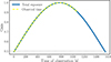 |
Fig. 1. Gain profile of an NC observation on 3XMM J185246.6+003317 as an example. The target has a total exposure of 1548 s every day. The exposure is defined as the amount of time per day during which the NC can observe the target with a gain ≳0.5 (the gray dashed line represents this limit). The plot shows in blue the NC gain profile, which corresponds to the primary beam attenuation, over the entire observable interval, while the dashed yellow line represents the net observed window that, for this target, is stopped at 480 s in advance due to schedule constraints. |
3.1. Data analysis strategy
The observations are stored as 16-bit SIGPROC filterbank format data (Lorimer 2011). The narrow bandwidth of the NC and the low presence of RFIs allowed us to analyze most of the filterbanks without using RFI cleaning tools. Anyway, when the individual filterbanks provided a high number of candidates due to RFI, we used the inter-quartile range mitigation (IQRM)6 real-time adaptive RFI masking (Morello et al. 2022). The incoherent de-dispersion and the search for radio transients were performed using the HEIMDALL7 algorithm (Barsdell et al. 2012). Taking into account the high uncertainties on the Galactic DM contribution (see Table 1), due to not well-known distances and different possible models, we searched for candidates over a wide DM range, from 20 to 3000 pc cm−3. We used a narrower DM range only in the case of SGR J1935+2154, between 300 to 360 pc cm−3, centered around the known DMJ1935 ∼ 332.7 pc cm−3 (CHIME/FRB Collaboration 2020). Our full use of our computing capabilities allowed us to perform a search adopting a fine DM sampling, with ∼25 000 DM steps (∼1100 in the case of SGR J1935+2154), and to look for bursts with a maximum width of ∼70 ms. The HEIMDALL-generated candidates with a signal-to-noise ratio greater than seven were classified with FETCH8, a convolutional neural network trained to distinguish between RFI and astrophysical de-dispersed signals (Agarwal et al. 2020). We tested the efficiency of FETCH models on NC data, and we found that combining the probabilities of the different models improves the detectability of dispersed signals. Finally, every candidate that passed all the selection steps underwent a deep human-based inspection.
3.2. Observing campaign
We observed the targets from 2024-01-27 to 2025-03-03 (see Fig. 2) with daily observations as allowed by the telescope’s scheduling constraints. In Table 2, we report the amount of observing time for each target. Most of the observed magnetars are distributed in the Galactic plane; therefore, the RA distribution of the targets is such that there is often overlap of visibility from the NC (see Fig. 3). Taking the overlaps of the targets and the movement delays of the antennas into account, we were forced to cut some of the observing intervals at the extremes. Cropping the observing windows reduced the amount of on-source time for the NC. However, the cutting of the extremes of the interval implies that the parts that are erased are those that are less sensitive due to primary beam attenuation (as shown in Fig. 1), and we have taken this into account in the results of our work.
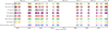 |
Fig. 2. Observing windows during the monitoring campaign. The total exposure time is 565.92 h. Each vertical notch represents an observation. The typical duration of a daily exposure for the different sources can be seen in Fig. 3. |
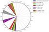 |
Fig. 3. Daily time distribution of the observable windows of the targets. The NC observing intervals on each target shift by ∼4 minutes per day in advance. |
4. Methods
If we apply Eq. (1) to our observing campaign, considering only candidates with S/N ≥ 7, the NC minimum detectable flux density is ![$ F_\nu \sim 7.55 \; \left(\frac{\mathit{w}}{\mathrm{[ms]}}\right)^{-1/2} \frac{1}{\mathcal{G}(\mathrm{ToA})} $](/articles/aa/full_html/2025/08/aa54386-25/aa54386-25-eq18.gif) Jy. If we convert the flux density into an energy for a source located at distance D using the NC bandwidth Δν = 14.815 MHz and assuming a pulse duration of w = 1 ms, we find the highest (𝒢(ToA) = 0.493) and lowest (𝒢(ToA) = 1) detectable energies:
Jy. If we convert the flux density into an energy for a source located at distance D using the NC bandwidth Δν = 14.815 MHz and assuming a pulse duration of w = 1 ms, we find the highest (𝒢(ToA) = 0.493) and lowest (𝒢(ToA) = 1) detectable energies:
![$$ \begin{aligned} E_{\mathrm{min} } = (1.34-2.72) \times 10^{20} \left(\frac{D}{\mathrm{[pc]}}\right)^{2} \; \mathrm{erg}. \end{aligned} $$](/articles/aa/full_html/2025/08/aa54386-25/aa54386-25-eq19.gif)
The intervals of the minimum detectable energies for each magnetar are listed in the third column of Table 2. The uncertainties on the distances of the targets (listed in Table 1) can influence the minimum energy estimates, but we verified that the final conclusions of this work are not significantly influenced by these changes even when assuming the extreme values.
Inferred upper limits on the sample of magnetars.
Our sensitivity threshold corresponds to a spectral luminosity of ∼7.3 × 10²² erg s−1 Hz−1 for a 1 ms burst assuming D = 2 kpc (i.e., the minimum distance in our sample of magnetars). On the other hand, when using the maximum distance among our targets, D = 12.5 kpc, the limit grows to ∼2.8 × 1024 erg s−1 Hz−1. Comparing our thresholds with the known population of fast (≲1 s) radio transients (Nimmo et al. 2022), we expected to be sensitive to any FRB-like event from our sample of magnetars. Furthermore, especially for the closest magnetars, the NC has the sensitivity to detect events with giant-pulse energy (Karuppusamy et al. 2010) as well as the most energetic single pulses from rotating radio transients and “ordinary” pulsars (Keane 2018).
Similar to Pelliciari et al. (2023), assuming an energy power-law distribution of single bursts, we defined the rate of events above the minimum detectable energy coming from a single magnetar in the primary beam attenuation interval, j, as
Different from Pelliciari et al. (2023), we did not restrict the rate of events to the ones with an energy higher than E0 (i.e., using the Heaviside function Θ[E − E0]). In fact, in our work the low-energy events strongly influence the expected bursts rate. In Eq. (3), we fit the NC gain profile (Fig. 1) by dividing it into short intervals. Therefore, Emin, j is the NC sensitivity in the gain interval, j, computed with Eq. (1). The maximum energy of the distribution is Emax, E0 is a reference energy used for the normalization, and K0 is a normalization constant that ensures the following:
The equation defines the number of events emitted by a magnetar with energy above E0. Importantly, the free parameters of our model are λmag and the power-law index γ. Similar to Pelliciari et al. (2023), we adopted a reference energy E0 = 3.2 × 1034 erg, which represents the energy of the FRB-like event of SGR J1935+2154 (Margalit et al. 2020) considering our 9 kpc assumption of the distance of SGR J1935+2154 (Pelliciari et al. 2023 assumed E0 = 2 × 1034 erg due to a different distance estimate). Furthermore, we assumed that the maximum energy a magnetar is able to emit depends on the energy reservoir of the neutron star, which is a function of the surface magnetic field strength (Margalit et al. 2020):
Taking into account the uncertainties on the radio efficiency and the complex magnetic field structure of magnetars, we used a common order of magnitude for the maximum energy for all the magnetars: Emax = 1.2 × 1041 erg. Here, we assumed a surface magnetic field of Bdip = 2 × 10¹⁴ G and η = 10−5 as the efficiency of the radio emission for each magnetar, as in the case of SGR J1935+2154 radio bursts (Margalit et al. 2020).
Combining the normalization of Eq. (4) with the rate of events of Eq. (3), we obtained
From this equation, knowing that in our case Emax ≫ E0 ≫ Emin, we could see that the choice of the maximum energy influences the inferred rate of events only when γ ≃ 1. If we perform a sum weighted on the time spent in every primary beam attenuation interval Tj, we obtain
![$$ \begin{aligned} \mathcal{R} \left(\lambda _{\mathrm{mag} },\gamma \right) = \lambda _{\mathrm{mag} } \frac{\sum _{j}\left[\left(E_{\mathrm{max} }^{\;\;\;\;1-\gamma } - E_{\mathrm{min} ,j}^{\;\;\;\;1-\gamma }\right) \cdot T_{j}\right]}{\left( E_{\mathrm{max} }^{\;\;\;\;1-\gamma } - E_{0}^{\;1-\gamma } \right) \cdot \sum _{j} \left[T_{j}\right]}\cdot \end{aligned} $$](/articles/aa/full_html/2025/08/aa54386-25/aa54386-25-eq24.gif)
Finally, in the case of the entire sample of magnetars, the rate of events expected from our sample is the sum of the rates of the single magnetars:
5. Results and discussion
No magnetar-related detections were found during the monitoring campaign. We exploited the observing hours to set upper limits on the burst rate of impulsive events from each target in our sample of Galactic magnetars. We assumed a Poisson distribution of events in time, and the inferred upper limits for each magnetar are listed in the fourth column of Table 2. Considering the entire ∼560 hours of monitoring, the upper limit on the burst rate at a 95% confidence level is ℛtot < 46 yr−1 (Gehrels 1986, Table 1). If we exclude the magnetar candidate SGR 2013+34, the “clean” upper limit increases to ℛtot, clean < 52 yr−1. The upper limits refer only to bursts with an energy greater than the minimum detectable energy for each magnetar. In fact, each target has a different minimum detectable energy interval and a different upper limit on the burst rate, which is related to the amount of on-source time.
The result of our power-law energy distribution model (see Sect. 4) is a rate of single pulse events, and it can be represented using a colored scale that shows the variations of the number of detectable events in the parameter space. The rate, ℛtot, is a function of the free parameters of the model, which are the slope of the power-law energy distribution (γ) and the number of events with energy greater than the energy emitted by the FRB-like event of SGR J1935+2154 (λmag). If we combine the number of observable events computed using the method described before (see Sect. 4) with the upper limits obtained by our observations, we can investigate the parameter space of our model and infer which are the favored combinations of the free parameters. The resulting plots for the entire magnetar sample are shown in Fig. 4, while the plots for each individual magnetar are reported in Appendix A for completeness.
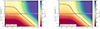 |
Fig. 4. Graphical representation of the power-law energy distribution model for both the entire sample of targets (left) and excluding the magnetar candidate SGR 2013+34 (right). The x-axis represents the slope of the power-law energy distribution γ, while on the y-axis are the number of events with an energy greater than the energy emitted by the FRB-like event of SGR J1935+2154 λmag. The two free parameters of the model are γ and λmag, and their combinations produce ℛtot (Eq. 8) for the entire magnetar sample, respectively. The rate of events obtained in every case are shown using a fixed logarithmic color code presented in the color bars. The solid black lines represent the upper limits obtained with our observing campaign on the possible combinations of γ and λmag, while the black dashed lines show reference values for graphical purposes. The difference between the upper and lower panels is the scale of the y-axis: The upper panels are in linear scale, and the lower panels are in logarithmic scale. |
In our model, the rate of high-energy events, λmag, has the role of a normalization. Therefore, having a flat energy distribution (i.e., a low γ) implies that we do not expect a large population of detectable low-energy events. On the other hand, rapidly decreasing power-law distributions (i.e., high γ) produce a large number of low-energy events that we expect are detectable. In Fig. 4, our results are combined with the upper limits of the observations, and the graphs suggest that flatter energy distributions are favored over steeper ones. We note that values of γ < 1 produce a flat upper limit in our plots since in that case, the Emax contribution dominates in Eq. (6).
Since the SGR J1935+2154 FRB-like event in 2020 (CHIME/FRB Collaboration 2020), a considerable effort has been made to investigate the possible link between magnetars and FRBs. Works such as CHIME/FRB Collaboration (2020), Kirsten et al. (2021), Pelliciari et al. (2023) have already set upper and lower limits on the expected burst rate of FRB-like signals from magnetars, while Xie et al. (2025) has set deep upper limits on the energy emitted by the magnetars SGR J1935+2154 and 3XMM J185246.6+003317 during quiescent phases.
Kirsten et al. (2021) used a few European radio telescopes to monitor the activity of SGR J1935+2154 and obtained two detections at 1.4 GHz in a total of 763.3 hours. Knowing that the time separation between the two detected bursts was only ∼1.4 s, they fit the time intervals between subsequent bursts with a Weibull distribution. On the other hand, in our case of nondetections, we assumed a Poissonian distribution of events as explained earlier. If we apply our statistics to the Kirsten et al. (2021) work and we ignore the statistical differences and the fact that both the observing frequency bands and sensitivities are different, we obtain an expected number of detectable events from magnetars between 4−34 yr−1 that is consistent with our upper limits.
If we take into account the literature observations on extragalactic targets, CHIME/FRB Collaboration (2020) observed SGR J1935+2154 and 15 nearby galaxies, and they set constraints on the burst rate of FRB-like events. They assumed a number of magnetars in the Milky Way (MW), Nmag ∼ 30, and that the number of magnetars in a galaxy is directly related to its star formation rate, resulting in a rate of SGR J1935+2154-like bursts per magnetar of 0.007 < λmag < 0.4 yr−1. A similar reasoning was followed in Pelliciari et al. (2023), from which a consistent upper limit of λmag < 0.42 yr−1 was obtained. We can use the constraints on λmag from CHIME/FRB Collaboration (2020) to investigate which combinations of our parameter space are favored by our upper limits. The resulting plot is shown in the left panel of Fig. 5, where we can observe that only power-law indexes γ ≲ 1.4 produce observable rates consistent with the constraints set by CHIME/FRB Collaboration (2020). Furthermore, we can exploit the ∼695 hours observed in the nearby galaxies campaign of Pelliciari et al. (2023) to obtain an improved NC upper limit on the burst rate, resulting in λmag < 0.043 yr−1. The resulting plot, compared with the literature upper limits, is shown in the right panel of Fig. 5. We used the same conservative assumptions of CHIME/FRB Collaboration (2020), Pelliciari et al. (2023) by setting the number of magnetars in the MW as Nmag = 29 but including the low-energy events (i.e., we removed the Heaviside function in Eq. 4 of Pelliciari et al. 2023). Crucially, Nmag = 29 is the number of known magnetars in our Galaxy, though we know that many more magnetars may actually be present in the MW. If we define magnetars as sources that can emit SGR-like flares, works such as Muno et al. (2008), Gullón et al. (2015), and Pardo et al. (in prep.) suggest that the number of currently active neutron stars in the MW that could behave as magnetars is between 500 and 800. Taking into account this estimate, the upper limit (solid black line) shown in the right panel of Fig. 5 is most likely overestimated. In our case, we note that if we adopt a value consistent with these population studies of Nmag = 500, we find a NC upper limit of λmag < 0.0025 yr−1.
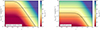 |
Fig. 5. Graphical representation of the power-law energy distribution model. The left panel is the same as the right panel of Figure 4. The dashed lines represent the CHIME/FRB Collaboration (2020) lower and upper limits at a 95% confidence level on the rate of events that are SGR J1935+2154-like. We adopted a different scale for better visualization. In the right panel, we combined our campaign with observations of nearby galaxies by Pelliciari et al. (2023). |
6. Summary and conclusions
In this work, we have used the NC radio telescope to monitor seven known Galactic magnetars that are visible from the site (Table 1). Our ∼560 hours of observations did not produce any sound detection of events directly linked to magnetars. We exploited our long-term monitoring campaign to constrain the rate of single pulses from this class of objects while also making considerations on the occurrence of FRB-like events. Our upper limit of < 52 yr−1 at a 95% confidence level on the cleaned sample of magnetars is consistent with the ones estimated in previous observations (Kirsten et al. 2021). Furthermore, we modeled the single pulse emission from magnetars using a power law energy distribution, similar to Pelliciari et al. (2023). Our upper limits constrain the free parameters of the model (γ and λmag), suggesting a flat energy distribution of events (see Table 2 and Fig. 4). If we include observations of nearby galaxies (CHIME/FRB Collaboration 2020; Pelliciari et al. 2023), the constraints on the rate become more stringent, and the flatter energy distributions are even more preferred (see Fig. 5). Furthermore, when adopting a more realistic estimate of the number of active magnetars in MW-like galaxies (Nmag = 500), the limits become even more stringent.
The fact that none of the targets showed X-ray bursting activity or outburst phases during our monitoring campaign could be a hint that FRB-like events are indeed related to magnetar-like activity windows, as in the case of SGR J1935+2154 and of their radio emission in general. As already discussed, the typical inferred luminosity of extragalactic FRBs is a few orders of magnitude higher than the FRB-like event observed from the magnetar SGR J1935+2154.
It is relevant to point out that our observations constrain λmag to be λmag < 7.4 yr−1 for flat values of the energy slope γ, that is γ ≲ 1.1. However, for steeper energy slopes (i.e., γ ≳ 1.4), the chance of observing an FRB-like event with energy greater than that of SGR J1935+2154 becomes increasingly small. Furthermore, if we combine our observations with observations of nearby galaxies (CHIME/FRB Collaboration 2020; Pelliciari et al. 2023), the constraint on λmag for the flat energy slopes becomes 0.007 < λmag < 0.043 yr−1.
These results are somewhat in tension with models that attempt to explain the all-sky FRB rate with radio bursts from magnetars similar to SGR J1935+2154. Indeed, James et al. (2022) found that the extragalactic FRB rate can be explained in terms of the evolution of the cosmic star formation rate, with a slope of the luminosity distribution γ ≃ 2.19. If there is no significant evolution of the slope with redshift, this result is disfavored by our observations that tend to exclude slopes steeper than ∼1.5.
Furthermore, Margalit et al. (2020), based on radio observations of SGR J1935+2154 (CHIME/FRB Collaboration 2020), assumed 0.0036 < λmag < 0.8 yr−1 and found that the slope of the luminosity distribution needs to be in the 1 < γ < 1.5 range to fit the extragalactic FRB rate. For this reason, they speculated on the existence of an additional population of more exotic magnetars not generated by core-collapse supernovae that may need to be included in the model, as the event rate of SGR J1935+2154-like magnetars is too small to account for the observed extragalactic rate. As our results reduce the ranges of allowed λmag and γ values, they imply a larger contribution from this possible population of exotic magnetars.
Possibly six, including SGR J1935+2154, which was detected only with FAST in a small fraction of their monitoring time (Zhu et al. 2023).
However, CHIME/FRB Collaboration (2023b) suggest a repeaters detection rate of ∼3%.
The typical localization accuracy is ∼2° (68% containment radius), see https://gammaray.nsstc.nasa.gov/batse/grb/rbr/
Acknowledgments
The reported data were collected during the phase of the INAF scientific exploitation with the NC radio telescope. We thank the referee, for their comments and suggestions that greatly improved the paper, and Nanda Rea, for useful discussion. This publication was produced while AG was attending the PhD program in Space Science and Technology at the University of Trento, Cycle XXXIX, with the support of a scholarship financed by the Ministerial Decree no. 118 of 2nd March 2023, based on the NRRP – funded by the European Union – NextGenerationEU – Mission 4 “Education and Research”, Component 1 “Enhancement of the offer of educational services: from nurseries to universities” – Investment 4.1 “Extension of the number of research doctorates and innovative doctorates for public administration and cultural heritage” – CUP E66E23000110001. Part of the research activities described in this paper were carried out with contribution of the NextGenerationEU funds within the National Recovery and Resilience Plan (PNRR), Mission 4 – Education and Research, Component 2 – From Research to Business (M4C2), Investment Line 3.1 – Strengthening and creation of Research Infrastructures, Project IR0000026 – Next Generation Croce del Nord.
References
- Agarwal, D., Aggarwal, K., Burke-Spolaor, S., Lorimer, D. R., & Garver-Daniels, N. 2020, MNRAS, 497, 1661 [Google Scholar]
- Bailes, M. 2022, Science, 378, abj3043 [NASA ADS] [CrossRef] [Google Scholar]
- Barsdell, B. R., Bailes, M., Barnes, D. G., & Fluke, C. J. 2012, MNRAS, 422, 379 [CrossRef] [Google Scholar]
- Barthelmy, S. D., Baumgartner, W. H., Beardmore, A. P., et al. 2008, ATel, 1676, 1 [Google Scholar]
- Bochenek, C. D., Ravi, V., Belov, K. V., et al. 2020, Nature, 587, 59 [NASA ADS] [CrossRef] [Google Scholar]
- Borghese, A., Coti Zelati, F., Israel, G. L., et al. 2022, MNRAS, 516, 602 [Google Scholar]
- Caleb, M., Rajwade, K., Desvignes, G., et al. 2022, MNRAS, 510, 1996 [Google Scholar]
- Camero, A., Papitto, A., Rea, N., et al. 2014, MNRAS, 438, 3291 [Google Scholar]
- Cameron, P. B., Chandra, P., Ray, A., et al. 2005, Nature, 434, 1112 [NASA ADS] [CrossRef] [PubMed] [Google Scholar]
- Camilo, F., Ransom, S. M., Halpern, J. P., et al. 2006, Nature, 442, 892 [NASA ADS] [CrossRef] [Google Scholar]
- Camilo, F., Ransom, S. M., Halpern, J. P., & Reynolds, J. 2007, ApJ, 666, L93 [NASA ADS] [CrossRef] [Google Scholar]
- CHIME/FRB Collaboration (Andersen, B. C., et al.) 2020, Nature, 587, 54 [Google Scholar]
- CHIME/FRB Collaboration (Amiri, M., et al.) 2023a, ApJS, 264, 53 [Google Scholar]
- CHIME/FRB Collaboration (Andersen, B. C., et al.) 2023b, ApJ, 947, 83 [NASA ADS] [CrossRef] [Google Scholar]
- CHIME/FRB Collaboration (Amiri, M., et al.) 2024, ApJ, 969, 145 [NASA ADS] [CrossRef] [Google Scholar]
- Chrimes, A. A., Levan, A. J., Lyman, J. D., et al. 2025, A&A, 696, A127 [NASA ADS] [CrossRef] [EDP Sciences] [Google Scholar]
- Cordes, J. M., & Lazio, T. J. W. 2002, ArXiv e-prints [arXiv:astro-ph/0207156] [Google Scholar]
- Coti Zelati, F., Rea, N., Pons, J. A., Campana, S., & Esposito, P. 2018, MNRAS, 474, 961 [NASA ADS] [CrossRef] [Google Scholar]
- Dall’Osso, S., & Stella, L. 2022, Astrophys. Space Sci. Lib., 465, 245 [Google Scholar]
- Davies, B., Figer, D. F., Kudritzki, R.-P., et al. 2009, ApJ, 707, 844 [NASA ADS] [CrossRef] [Google Scholar]
- Dhillon, V. S., Marsh, T. R., Littlefair, S. P., et al. 2011, MNRAS, 416, L16 [Google Scholar]
- Dib, R., & Kaspi, V. M. 2014, ApJ, 784, 37 [NASA ADS] [CrossRef] [Google Scholar]
- Durant, M., & van Kerkwijk, M. H. 2006, ApJ, 650, 1070 [Google Scholar]
- Esposito, P., Israel, G. L., Zane, S., et al. 2008, MNRAS, 390, L34 [NASA ADS] [Google Scholar]
- Esposito, P., Israel, G. L., Turolla, R., et al. 2010, MNRAS, 405, 1787 [NASA ADS] [Google Scholar]
- Esposito, P., Rea, N., Borghese, A., et al. 2020, ApJ, 896, L30 [NASA ADS] [CrossRef] [Google Scholar]
- Esposito, P., Rea, N., & Israel, G. L. 2021, Astrophys. Space Sci. Lib., 461, 97 [NASA ADS] [CrossRef] [Google Scholar]
- Fahlman, G. G., & Gregory, P. C. 1981, Nature, 293, 202 [Google Scholar]
- Foley, S., Kouveliotou, C., Kaneko, Y., & Collazzi, A. 2012, GRB Coordinates Network, 13280, 1 [Google Scholar]
- Frail, D. A., Kulkarni, S. R., & Bloom, J. S. 1999, Nature, 398, 127 [Google Scholar]
- Gehrels, N. 1986, ApJ, 303, 336 [Google Scholar]
- Göǧüş, E., Kouveliotou, C., Woods, P. M., et al. 2001, ApJ, 558, 228 [Google Scholar]
- Gullón, M., Pons, J. A., Miralles, J. A., et al. 2015, MNRAS, 454, 615 [CrossRef] [Google Scholar]
- Gupta, O., Beniamini, P., Kumar, P., & Finkelstein, S. L. 2025, ApJ, 986, 100 [Google Scholar]
- He, C., Ng, C. Y., & Kaspi, V. M. 2013, ApJ, 768, 64 [NASA ADS] [CrossRef] [Google Scholar]
- Hulleman, F., van Kerkwijk, M. H., & Kulkarni, S. R. 2000, Nature, 408, 689 [Google Scholar]
- Hulleman, F., van Kerkwijk, M. H., & Kulkarni, S. R. 2004, A&A, 416, 1037 [NASA ADS] [CrossRef] [EDP Sciences] [Google Scholar]
- Hurley, K., Cline, T., Mazets, E., et al. 1999a, Nature, 397, 41 [NASA ADS] [CrossRef] [Google Scholar]
- Hurley, K., Li, P., Kouveliotou, C., et al. 1999b, ApJ, 510, L111 [NASA ADS] [CrossRef] [Google Scholar]
- Ibrahim, A. Y., Borghese, A., Coti Zelati, F., et al. 2024, ApJ, 965, 87 [Google Scholar]
- Israel, G. L., Mereghetti, S., & Stella, L. 1994, ApJ, 433, L25 [Google Scholar]
- Israel, G. L., Romano, P., Mangano, V., et al. 2008, ApJ, 685, 1114 [Google Scholar]
- Israel, G. L., Esposito, P., Rea, N., et al. 2016, MNRAS, 457, 3448 [NASA ADS] [CrossRef] [Google Scholar]
- Israel, G. L., Burgay, M., Rea, N., et al. 2021, ApJ, 907, 7 [NASA ADS] [CrossRef] [Google Scholar]
- James, C. W., Prochaska, J. X., Macquart, J. P., et al. 2022, MNRAS, 510, L18 [Google Scholar]
- Karuppusamy, R., Stappers, B. W., & van Straten, W. 2010, A&A, 515, A36 [NASA ADS] [CrossRef] [EDP Sciences] [Google Scholar]
- Kaspi, V. M., & Beloborodov, A. M. 2017, ARA&A, 55, 261 [Google Scholar]
- Keane, E. F. 2018, Nat. Astron., 2, 865 [Google Scholar]
- Kirsten, F., Snelders, M. P., Jenkins, M., et al. 2021, Nat. Astron., 5, 414 [Google Scholar]
- Kothes, R., & Foster, T. 2012, ApJ, 746, L4 [Google Scholar]
- Kothes, R., Sun, X., Gaensler, B., & Reich, W. 2018, ApJ, 852, 54 [NASA ADS] [CrossRef] [Google Scholar]
- Kouveliotou, C., Strohmayer, T., Hurley, K., et al. 1999, ApJ, 510, L115 [NASA ADS] [CrossRef] [Google Scholar]
- Kramer, M., Stappers, B. W., Jessner, A., Lyne, A. G., & Jordan, C. A. 2007, MNRAS, 377, 107 [Google Scholar]
- Levin, L., Bailes, M., Bates, S., et al. 2010, ApJ, 721, L33 [Google Scholar]
- Lin, L., Kouveliotou, C., Baring, M. G., et al. 2011, ApJ, 739, 87 [Google Scholar]
- Locatelli, N. T., Bernardi, G., Bianchi, G., et al. 2020, MNRAS, 494, 1229 [NASA ADS] [CrossRef] [Google Scholar]
- Lorimer, D. R. 2011, Astrophysics Source Code Library [record ascl:1107.016] [Google Scholar]
- Lorimer, D. R., & Kramer, M. 2012, Handbook of Pulsar Astronomy (Cambridge: Cambridge University Press) [Google Scholar]
- Lorimer, D. R., Bailes, M., McLaughlin, M. A., Narkevic, D. J., & Crawford, F. 2007, Science, 318, 777 [Google Scholar]
- Lundgren, S. C., Cordes, J. M., Ulmer, M., et al. 1995, ApJ, 453, 433 [Google Scholar]
- Margalit, B., Beniamini, P., Sridhar, N., & Metzger, B. D. 2020, ApJ, 899, L27 [NASA ADS] [CrossRef] [Google Scholar]
- Mazets, E. P., Golentskii, S. V., Ilinskii, V. N., Aptekar, R. L., & Guryan, I. A. 1979a, Nature, 282, 587 [NASA ADS] [CrossRef] [Google Scholar]
- Mazets, E. P., Golenetskij, S. V., & Guryan, Y. A. 1979b, Sov. Astron. Lett., 5, 343 [NASA ADS] [Google Scholar]
- Mereghetti, S. 2008, A&ARv, 15, 225 [NASA ADS] [CrossRef] [Google Scholar]
- Mereghetti, S., Esposito, P., Tiengo, A., et al. 2006, ApJ, 653, 1423 [NASA ADS] [CrossRef] [Google Scholar]
- Mereghetti, S., Savchenko, V., Ferrigno, C., et al. 2020, ApJ, 898, L29 [Google Scholar]
- Morello, V., Rajwade, K. M., & Stappers, B. W. 2022, MNRAS, 510, 1393 [Google Scholar]
- Morii, M., Kawai, N., & Shibazaki, N. 2005, ApJ, 622, 544 [Google Scholar]
- Muno, M. P., Gaensler, B. M., Nechita, A., Miller, J. M., & Slane, P. O. 2008, ApJ, 680, 639 [Google Scholar]
- Nimmo, K., Hessels, J. W. T., Kirsten, F., et al. 2022, Nat. Astron., 6, 393 [NASA ADS] [CrossRef] [Google Scholar]
- Olausen, S. A., & Kaspi, V. M. 2014, ApJS, 212, 6 [Google Scholar]
- Palmer, D. M., Barthelmy, S., Gehrels, N., et al. 2005, Nature, 434, 1107 [NASA ADS] [CrossRef] [Google Scholar]
- Pelliciari, D., Bernardi, G., Pilia, M., et al. 2023, A&A, 674, A223 [NASA ADS] [CrossRef] [EDP Sciences] [Google Scholar]
- Pelliciari, D., Bernardi, G., Pilia, M., et al. 2024, A&A, 690, A219 [NASA ADS] [CrossRef] [EDP Sciences] [Google Scholar]
- Pizzocaro, D., Tiengo, A., Mereghetti, S., et al. 2019, A&A, 626, A39 [NASA ADS] [CrossRef] [EDP Sciences] [Google Scholar]
- Platts, E., Weltman, A., Walters, A., et al. 2019, Phys. Rep., 821, 1 [NASA ADS] [CrossRef] [Google Scholar]
- Pleunis, Z., Good, D. C., Kaspi, V. M., et al. 2021, ApJ, 923, 1 [NASA ADS] [CrossRef] [Google Scholar]
- Popov, S. B., Postnov, K. A., & Pshirkov, M. S. 2018, Phys. Usp., 61, 965 [CrossRef] [Google Scholar]
- Ranasinghe, S., Leahy, D. A., & Tian, W. 2018, Open. Phys. J., 4, 1 [Google Scholar]
- Rea, N., & Esposito, P. 2011, Astrophys. Space Sci. Proc., 21, 247 [NASA ADS] [CrossRef] [Google Scholar]
- Rea, N., Nichelli, E., Israel, G. L., et al. 2007, MNRAS, 381, 293 [Google Scholar]
- Rea, N., Israel, G. L., Turolla, R., et al. 2009, MNRAS, 396, 2419 [NASA ADS] [CrossRef] [Google Scholar]
- Rea, N., Esposito, P., Turolla, R., et al. 2010, Science, 330, 944 [NASA ADS] [CrossRef] [Google Scholar]
- Rea, N., Esposito, P., Pons, J. A., et al. 2013a, ApJ, 775, L34 [Google Scholar]
- Rea, N., Israel, G. L., Pons, J. A., et al. 2013b, ApJ, 770, 65 [NASA ADS] [CrossRef] [Google Scholar]
- Rea, N., Viganò, D., Israel, G. L., Pons, J. A., & Torres, D. F. 2014, ApJ, 781, L17 [NASA ADS] [CrossRef] [Google Scholar]
- Rehan, N. S., & Ibrahim, A. I. 2025, ApJS, 276, 60 [Google Scholar]
- Remazeilles, M., Dickinson, C., Banday, A. J., Bigot-Sazy, M. A., & Ghosh, T. 2015, MNRAS, 451, 4311 [NASA ADS] [CrossRef] [Google Scholar]
- Ryder, S. D., Bannister, K. W., Bhandari, S., et al. 2023, Science, 382, 294 [NASA ADS] [CrossRef] [Google Scholar]
- Sakamoto, T., Barbier, L., Barthelmy, S. D., et al. 2011a, Adv. Space Res., 47, 1346 [Google Scholar]
- Sakamoto, T., Barthelmy, S. D., Baumgartner, W. H., et al. 2011b, ApJS, 195, 2 [Google Scholar]
- Tavani, M., Casentini, C., Ursi, A., et al. 2021, Nat. Astron., 5, 401 [NASA ADS] [CrossRef] [Google Scholar]
- Tendulkar, S. P., Cameron, P. B., & Kulkarni, S. R. 2013, ApJ, 772, 31 [Google Scholar]
- Trudu, M., Pilia, M., Bernardi, G., et al. 2022, MNRAS, 513, 1858 [NASA ADS] [CrossRef] [Google Scholar]
- Turolla, R., Zane, S., & Watts, A. L. 2015, Rep. Progr. Phys., 78, 116901 [Google Scholar]
- van der Horst, A. J., Connaughton, V., Kouveliotou, C., et al. 2010, ApJ, 711, L1 [Google Scholar]
- Woods, P. M., Kaspi, V. M., Thompson, C., et al. 2004, ApJ, 605, 378 [Google Scholar]
- Xie, L., Han, J. L., Yang, Z. L., et al. 2025, RAA, 25, 014004 [Google Scholar]
- Xu, Y., Reid, M. J., Zheng, X. W., & Menten, K. M. 2006, Science, 311, 54 [NASA ADS] [CrossRef] [Google Scholar]
- Xu, J., Feng, Y., Li, D., et al. 2023, Universe, 9, 330 [Google Scholar]
- Yao, J. M., Manchester, R. N., & Wang, N. 2017, ApJ, 835, 29 [NASA ADS] [CrossRef] [Google Scholar]
- Zhang, B. 2023, Rev. Mod. Phys., 95, 035005 [NASA ADS] [CrossRef] [Google Scholar]
- Zhong, S.-Q., Dai, Z.-G., Zhang, H.-M., & Deng, C.-M. 2020, ApJ, 898, L5 [NASA ADS] [CrossRef] [Google Scholar]
- Zhou, P., Chen, Y., Li, X.-D., et al. 2014, ApJ, 781, L16 [CrossRef] [Google Scholar]
- Zhu, W., Xu, H., Zhou, D., et al. 2023, Sci. Adv., 9, eadf6198 [NASA ADS] [CrossRef] [Google Scholar]
Appendix A: Individual magnetar results
In Fig. A.1, we report on our results for each individual target, obtained using Eq. 7.
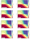 |
Fig. A.1. Graphical representation of the power-law energy distribution model for each magnetar in our sample. The x-axis represents the slope of the power-law energy distribution γ, while on the y-axis are the number of events with an energy greater than the energy emitted by the FRB-like event of SGR J1935+2154 λmag. The rate of events obtained in every case are shown using a fixed logarithmic color code presented in the color bars. The black line represents the upper limits obtained with our observing campaign on the possible combinations of γ and λmag, while the black dashed lines show reference values for graphical purposes. The difference between the upper and lower panels is the scale of the y-axis: The upper panels are in linear scale, and the lower panels are in logarithmic scale. |
All Tables
All Figures
|
Fig. 1. Gain profile of an NC observation on 3XMM J185246.6+003317 as an example. The target has a total exposure of 1548 s every day. The exposure is defined as the amount of time per day during which the NC can observe the target with a gain ≳0.5 (the gray dashed line represents this limit). The plot shows in blue the NC gain profile, which corresponds to the primary beam attenuation, over the entire observable interval, while the dashed yellow line represents the net observed window that, for this target, is stopped at 480 s in advance due to schedule constraints. |
| In the text | |
|
Fig. 2. Observing windows during the monitoring campaign. The total exposure time is 565.92 h. Each vertical notch represents an observation. The typical duration of a daily exposure for the different sources can be seen in Fig. 3. |
| In the text | |
|
Fig. 3. Daily time distribution of the observable windows of the targets. The NC observing intervals on each target shift by ∼4 minutes per day in advance. |
| In the text | |
|
Fig. 4. Graphical representation of the power-law energy distribution model for both the entire sample of targets (left) and excluding the magnetar candidate SGR 2013+34 (right). The x-axis represents the slope of the power-law energy distribution γ, while on the y-axis are the number of events with an energy greater than the energy emitted by the FRB-like event of SGR J1935+2154 λmag. The two free parameters of the model are γ and λmag, and their combinations produce ℛtot (Eq. 8) for the entire magnetar sample, respectively. The rate of events obtained in every case are shown using a fixed logarithmic color code presented in the color bars. The solid black lines represent the upper limits obtained with our observing campaign on the possible combinations of γ and λmag, while the black dashed lines show reference values for graphical purposes. The difference between the upper and lower panels is the scale of the y-axis: The upper panels are in linear scale, and the lower panels are in logarithmic scale. |
| In the text | |
|
Fig. 5. Graphical representation of the power-law energy distribution model. The left panel is the same as the right panel of Figure 4. The dashed lines represent the CHIME/FRB Collaboration (2020) lower and upper limits at a 95% confidence level on the rate of events that are SGR J1935+2154-like. We adopted a different scale for better visualization. In the right panel, we combined our campaign with observations of nearby galaxies by Pelliciari et al. (2023). |
| In the text | |
|
Fig. A.1. Graphical representation of the power-law energy distribution model for each magnetar in our sample. The x-axis represents the slope of the power-law energy distribution γ, while on the y-axis are the number of events with an energy greater than the energy emitted by the FRB-like event of SGR J1935+2154 λmag. The rate of events obtained in every case are shown using a fixed logarithmic color code presented in the color bars. The black line represents the upper limits obtained with our observing campaign on the possible combinations of γ and λmag, while the black dashed lines show reference values for graphical purposes. The difference between the upper and lower panels is the scale of the y-axis: The upper panels are in linear scale, and the lower panels are in logarithmic scale. |
| In the text | |
Current usage metrics show cumulative count of Article Views (full-text article views including HTML views, PDF and ePub downloads, according to the available data) and Abstracts Views on Vision4Press platform.
Data correspond to usage on the plateform after 2015. The current usage metrics is available 48-96 hours after online publication and is updated daily on week days.
Initial download of the metrics may take a while.