A diversity of starburst-triggering mechanisms in interacting galaxies and their signatures in CO emission

F. Renaud; F. Bournaud; O. Agertz; K. Kraljic; E. Schinnerer; A. Bolatto; E. Daddi; A. Hughes

doi:10.1051/0004-6361/201935222

Home

All issues

Volume 625 (May 2019)

A&A, 625 (2019) A65

Full HTML

Free Access

Issue		A&A Volume 625, May 2019


Article Number		A65
Number of page(s)		15
Section		Extragalactic astronomy
DOI		https://doi.org/10.1051/0004-6361/201935222
Published online		13 May 2019

A&A 625, A65 (2019)

A diversity of starburst-triggering mechanisms in interacting galaxies and their signatures in CO emission

F. Renaud¹, F. Bournaud², O. Agertz¹, K. Kraljic³, E. Schinnerer⁴, A. Bolatto⁵, E. Daddi² and A. Hughes⁶

¹ Department of Astronomy and Theoretical Physics, Lund Observatory, Box 43, 221 00 Lund, Sweden
e-mail: florent@astro.lu.se
² Laboratoire AIM Paris-Saclay, CEA/IRFU/SAp, Université Paris Diderot, 91191 Gif-sur-Yvette Cedex, France
³ Institute for Astronomy, University of Edinburgh, Royal Observatory, Blackford Hill, Edinburgh EH9 3HJ, UK
⁴ Max-Planck-Institut für Astronomie/Königstuhl 17, 69117 Heidelberg, Germany
⁵ Department of Astronomy, University of Maryland, College Park, MA 20742, USA
⁶ Institut de Recherche en Astrophysique et Planétologie (IRAP), CNRS, 14 avenue Belin, 31400 Toulouse, France

Received: 6 February 2019
Accepted: 21 March 2019

Abstract

The physical origin of enhanced star formation activity in interacting galaxies remains an open question. Knowing whether starbursts are triggered by an increase in the quantity of dense gas or an increase in the star formation efficiency therein would improve our understanding of galaxy evolution and make it possible to transfer the results obtained in the local Universe to high-redshift galaxies. In this paper, we analyze a parsec-resolution simulation of a model of interacting galaxies similar to the Antennae Galaxies. We find that the interplay of physical processes such as tides, shear, and turbulence shows complex and important variations in time and space, but that different combinations of these processes can produce similar signatures in observable quantities such as the depletion time and CO emission. Some clouds within the interacting galaxies exhibit an excess of dense gas (> 10⁴ cm⁻³), while others only attain similarly high densities in the tail of their density distribution. The clouds with an excess of dense gas are found across all regions of the galaxies, but their number density varies between regions due to different cloud assembly mechanisms. This translates into variations in the scale dependence of quantities related to cloud properties and star formation. The super-linearity of the relationship between the star formation rate and gas density implies that the dense gas excess corresponds to a decrease in the depletion time, and thus leads to a deviation from the classical star formation regime that is visible up to galactic scales. We find that the α_CO conversion factor between the CO luminosity and molecular gas mass exhibits stronger spatial than temporal variations in a system like the Antennae. Our results raise several caveats for the interpretation of observations of unresolved star-forming regions, but also predict that the diversity of environments for star formation will be better captured by the future generations of instruments.

Key words: methods: numerical / galaxies: star formation / galaxies: ISM

© ESO 2019

1. Introduction

In the local Universe, galaxy interactions and mergers are often associated with an enhancement of the star formation activity, particularly visible in ultraluminous infrared galaxies (ULIRGs; Sanders & Mirabel 1996; Scudder et al. 2012; Knapen et al. 2015). Although this is now routinely reproduced in simulations (e.g., Karl et al. 2010; Teyssier et al. 2010; Moreno et al. 2013; Renaud et al. 2014), the underlying physical reasons and the main driver(s) of these starbursts remain uncertain. Understanding the physics of enhanced star formation is key to establishing whether and how the known empirical and theoretical relations between star formation and its triggers derived in the local Universe can be transposed to the extreme conditions at high redshift, during the first phases of galaxy formation.

To date, it is not clear whether the bursts of star formation rate (SFR) result from an enhancement of the quantity of dense gas due to a compression from galactic scale mechanisms (e.g., Combes et al. 1994; Casasola et al. 2004; Kaneko et al. 2017) or from an increase in the efficiency of the formation process itself¹ (see Solomon & Sage 1988; Graciá-Carpio et al. 2008; Michiyama et al. 2016). The former is often quantified by estimating the molecular gas mass, while the latter relates to the depletion time of the gas reservoir (t_dep = M_gas/SFR). A number of observations of local interacting systems have quantified the variations in these two quantities to determine the main driver of starbursts, often as functions of the interaction parameters. The emergent consensus depicts a mixed influence of the two effects, with the increase in dense gas content being the dominant one (Pan et al. 2018).

In the Schmidt–Kennicutt plane (i.e., the relation between the surface densities of gas and of SFR), an increase in the dense gas mass leads to the expected increase in SFR along the canonical relation( $Σ_{gas} \propto Σ_{SFR}^{N}$ ${\Sigma _{{\rm{gas}}}} \propto \Sigma _{{\rm{SFR}}}^N$ , with N ≈ 1.4−2.3, Kennicutt 1998; Kennicutt & Evans 2012; Kravtsov 2003; Elmegreen & Elmegreen 2005; Semenov et al. 2018), i.e., at a roughly uniform depletion time (∼1 Gyr, Bigiel et al. 2010; Saintonge et al. 2011; Leroy et al. 2013). Such a high dense gas mass is what is observed, for example in gas-rich turbulent disk galaxies at redshifts z ≳ 1 (e.g., Tacconi et al. 2010). However, a decrease in the depletion time as observed, for example, in LIRGs (Klaas et al. 2010; Martinez-Badenes et al. 2012; Nehlig et al. 2016), translates into a deviation from this relation. A duality of star formation regimes has been proposed by Daddi et al. (2010a, see also Genzel et al. 2010) to distinguish galaxies with long and short depletion times, respectively disks and mergers, but independently of their SFRs. To reach this conclusion, these authors had to assume a conversion factor α_CO between the CO luminosity and the molecular mass (due to the difficulty in detecting H₂; see Bolatto et al. 2013). Uncertainties hinder the choice of this factor (Zhu et al. 2003; Graciá-Carpio et al. 2008; Pereira-Santaella et al. 2016). The value of 0.8 M_⊙ K⁻¹ km⁻¹ s⁻¹ pc⁻² adopted by Daddi et al. for the mergers is in sharp contrast with that of the disks (4.3 for the Milky Way) and has been highly debated; an underestimated α_CO would artificially accentuate or even create the differences between the regimes in depletion times. However, the decrease in t_dep is retrieved in parsec-resolution simulations of interacting galaxies where the transitions between the disk and the merger regimes (and back) can be resolved without any assumptions about α_CO (Renaud et al. 2014, 2018; Kraljic 2014; Fensch et al. 2017). Furthermore, by post-processing similar simulations to derive α_CO, Renaud et al. (2019) showed that the choice of a low α_CO for ULIRG systems is likely justified (see also Narayanan et al. 2011) for a few 10 Myr after the peak(s) of their SFRs. The positions of starbursting systems (at least in the local Universe) in the Schmidt–Kennicutt plane thus confirm both an increase in the dense gas content and a decrease in the depletion time. We note that this effect is hidden in variants of this diagram when Σ_gas is normalized by the free-fall time (Krumholz et al. 2012; Federrath 2013; Salim et al. 2015).

Variations in the depletion time have been reported observationally across galactic disks (e.g., Meidt et al. 2013; Bigiel et al. 2015; Usero et al. 2015; Pereira-Santaella et al. 2016; Saito et al. 2016; Leroy et al. 2017; Tomičić et al. 2018; Bemis & Wilson 2019) and along the course of interactions both theoretically (e.g., Renaud et al. 2014) and observationally by considering statistical samples of galaxies at different evolutionary stages (e.g., Feldmann et al. 2012; Violino et al. 2018; Pan et al. 2018). For instance, the evolution of modeled interacting systems in the Schmidt–Kennicutt plane reveals that successive encounters do not induce the same effects (see, e.g., Fig. 3 in Renaud et al. 2014 for an Antennae-like system, and Fig. 11 in Renaud et al. 2018 for a Cartwheel-like galaxy). Distant passages (usually at an early stage of the interaction before strong dynamical friction has reduced the orbital energy) trigger a violent increase in the star formation activity over large volumes, while the global surface density of gas remains almost unchanged (measured at a scale of ∼100 pc). However, closer, penetrating encounters (usually at later stages, moments before coalescence) yield an increase in the gas density and in the star formation rate density, because most of the activity is concentrated in the galactic nuclei. Differences are also seen in star cluster formation rates, in the sense that clusters are preferentially formed during early passages rather than at coalescence (Renaud et al. 2015a).

These variations in both space and time relate to extended star formation, in particular the off-nuclear activity (Barnes 2004; Wang et al. 2004; Cullen et al. 2006; Smith et al. 2008; Hancock et al. 2009; Chien & Barnes 2010), and suggest that different physical mechanisms trigger starburst events through an increase in the dense gas mass, a decrease in the depletion time, or both, and that their interplay and relative importance vary in space and time as a function of the properties of the galactic encounter. For instance, the importance of nuclear inflows induced by tidal torques from one galaxy onto the other (Keel et al. 1985; Barnes & Hernquist 1991) increases with decreasing pericenter distance. Similarly, shocks have a strong impact during close passages when the dense regions of the interstellar medium (ISM) overlap (Jog & Solomon 1992). Conversely, tidal and turbulent compression found in simulations (Renaud et al. 2014) are of gravitational origin and are thus remote effects, occurring even during fly-bys and spanning large volumes. Understanding these phenomena, their interplay, and their possible observable signatures is thus important in order to pin down the physics of star formation and to determine which quantities should be the priority for future observational tests.

To address this problem with simulations, parsec-resolution is necessary to capture the cold, dense (∼10 K, ≳10³ cm⁻³) phase of the ISM, and the details of its turbulent nature. The high cost of these simulations caps the number of cases that can be studied. Here we use an Antennae-like simulation that encompasses a wide variety of star-forming environments (nuclei, shocks, extended formation). We explore these spatial variations, attempt to connect them to underlying physical process(es), and seek possible differences in their signatures in the CO emission that can be observed in real galaxies. Such differences may provide useful diagnostics for distant unresolved systems for which only integrated fluxes are available.

2. Method

2.1. Numerical method

The numerical method followed is identical to that used in Renaud et al. (2019), and is summarized here. The simulation considered is a hydrodynamical model of an Antennae-like major merger (see details and initial conditions in Renaud et al. 2015a), run with the adaptive mesh refinement code RAMSES (Teyssier 2002). It follows a quasi-Lagrangian refinement strategy: refinement occurs when a cell contains more than 50 particles (dark matter or stars from the initial conditions), when the baryonic density exceeds a certain value (which depends on the refinement level of the cell), or when the Jeans length is not resolved by at least four cells. Following this strategy, the maximum resolution reached is 1.5 pc. The metallicity is set uniformly at the solar value and no enrichment is considered. Heating and cooling are treated with a background UV heating, and atomic and molecular cooling from tabulated data (from Sutherland & Dopita 1993 and Rosen & Bregman 1995 at high and low temperatures, respectively). Star formation proceeds at an efficiency of 2% per free-fall time for the gas denser than 50 cm⁻³ (i.e., where the molecular gas fraction is expected to be close to unity at solar metallicity, Krumholz & Gnedin 2011). Photo-ionization from young stars is treated by heating the gas in Strömgren spheres, radiative pressure is deposited as momentum in this volume (see Renaud et al. 2013 for details), and type II supernova feedback is injected in the form of thermal energy (Dubois & Teyssier 2008; Teyssier et al. 2013).

The overall energy and momentum budgets of stellar feedback are still subjects to debate. The net effect of feedback has been shown to vary with the individual processes considered and the numerical scheme employed (e.g., Agertz et al. 2013; Hopkins et al. 2013a, 2018). Uncertainties and missing physics are partly accounted for in subgrid models by using correction parameters, yet lacking constraints (e.g., a factor modeling multiple scattering of photons in models of radiative pressure, see Krumholz & Matzner 2009; Krumholz & Dekel 2010). Furthermore, the effects of feedback on the surroundings of molecular clouds and the diffuse gas depend on the drift of stars from their formation sites (Renaud et al. 2013) and porosity of the ISM (e.g., Rogers & Pittard 2013; Ohlin et al. 2019). These aspects are not captured by most galaxy and cosmological simulations. Subgrid recipes should then include a parametrization of such effects that vary from low-redshift disks to more turbulent cases like interactions and high-redshift galaxies, but we currently lack observational constraints and/or derivations from first principles to improve our models. Details in our simulations would likely change with different treatments of feedback. However, we can argue that the star formation sites considered here are denser and more massive than in isolated galaxies, and thus are the least sensitive to feedback disruptions, in particular at pre-supernova stages (e.g., Matzner 2002; Dale et al. 2012). However, the enhanced star formation activity in a merger induces a larger deposition of energy and momentum, and the net result is uncertain at our working resolutions. Furthermore, neglecting AGN feedback in interacting galaxies might be critical as it could regulate star formation, in particular at the late stages of the merger (Hopkins et al. 2013b). Although this could affect our conclusions, in particular in the nuclear regions of the galaxies where X-ray photons could heat the gas and excite CO (e.g., Krips et al. 2011), the presence of an AGN in the Antennae galaxies has not been unambiguously established (see Brandl et al. 2009, and also Ueda et al. 2012, where the possibility of a hidden AGN causing high line ratios in the nucleus of NGC 4039 is presented).

The results related to star formation depend on the subgrid recipe used, and the details change when using different methods. The implementation and parameters we use have been designed, at our working resolution, to reproduce observations of integrated quantities like the SFR and the depletion time of the progenitor galaxies run in isolation, typical of main sequence galaxies. The simulation also retrieves the observed star formation activity of the Antennae during the interaction (see below). Uncertainties remain about the validity of non-integrated quantities like the number, spatial distribution, and masses of star-forming clouds that would change, for example by varying the density threshold and star formation efficiency (SFE), even if the SFR were unchanged. However, the morphology of the star-forming areas and the properties of the young massive clusters formed in the simulation are consistent with the observations (Renaud et al. 2015a), such that our models can be used to guide the interpretation of observational data down to a limiting scale of ∼10 pc.

2.2. CO emission

To compute the intensity of the CO (J → J − 1) emission lines, we first estimate the intrinsic emission on a cell basis, using the local density, temperature, and metallicity (fixed at the solar value in our case) of the ISM and lookup data (Weiß et al. 2005). The intrinsic line width is computed from the local velocity dispersion measured in the simulation. Then the net emission is evaluated by examining the velocity differences between the emitting cell and all the foreground cells along the same line of sight. The flux is absorbed if the velocity difference if smaller than the emitted line width (see Bournaud et al. 2015 for details). The process is repeated for all the cells in the simulations. The analysis is conducted at 1.5 pc resolution for almost all the lines of sight, with rare exceptions at 3 pc where the highest densities are not present. Data presented here are velocity-integrated Rayleigh-Jeans brightness temperatures, in units of K km s⁻¹. For convenience, we also provide the conversion to flux integral in units of Jy km s⁻¹. The CO-to-H₂ conversion factor α_CO (expressed in M_⊙ K⁻¹ km⁻¹ s⁻¹ pc⁻² in the rest of the paper) is inferred using the mass of the gas denser than 50 cm⁻³ (i.e., matching the star formation density threshold), which leads to a good agreement with empirical values for a Milky Way-like galaxy (Renaud et al. 2019). The dispersions presented are the root mean square values of a sample of five lines of sight, obtained by tilting the system by ±15° along the axes of the plane of the sky.

2.3. Regions of interest

After exploring the time evolution of the system in Renaud et al. (2014, 2019), we now focus on the snapshot representing the best morphological match to observational data. This instant is found 5 Myr after the second pericenter passage, and 19 Myr before the third pericenter passage which marks the onset of final coalescence. At this time, the SFR of the entire system reaches 15.7 M_⊙ yr⁻¹ (i.e., in the range of the observed values, 7−20 M_⊙ yr⁻¹, see Zhang et al. 2001; Brandl et al. 2009; Klaas et al. 2010) and the global α_CO is 2.9 (which puts the system in the post-burst regime; see Renaud et al. 2019).

For the sake of simplicity, we adopt a line of sight and an orientation comparable to that of the real system. In this snapshot, we select four star-forming regions of 1 kpc × 1 kpc, as shown in Fig. 1. The selection comprises the two galactic nuclei, the overlap region (on the eastern side, left in Fig. 1, where the disk remnants mix), and the arc on the opposite side of the overlap in the northern galaxy. In the real Antennae galaxies, the corresponding regions yield strong CO(1–0) emission (Wilson et al. 2003), and host – or have recently hosted – an intense star formation activity, in particular in the form of massive star clusters (≈5−10 Myr old; see, e.g., Whitmore et al. 1999; Bastian et al. 2009; Herrera et al. 2012). Our previous explorations of the system as a whole suggest that a variety of physical processes are responsible for this activity (Renaud et al. 2014, 2015a). In this paper, we seek observational signatures of these ISM processes, and in particular whether they affect the properties of the CO emission.

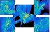Fig. 1.

Gas density map of the central 12 kpc × 12 kpc of the merger. The connections with the long tidal tails are visible on the left-hand side. The smaller panels show magnifications of the four 1 kpc × 1 kpc regions where our analysis is conducted.

For comparison, we also use another snapshot of the same simulation, during the starburst episode triggered by coalescence, when the SFR peaks at 97.2 M_⊙ yr⁻¹. We refer to this point as “ULIRG” in the following. We also include the Milky Way-like case (1 M_⊙ yr⁻¹) and the gas-rich clumpy galaxy (45 M_⊙ yr⁻¹, representing a disk at redshift ∼2) presented in Bournaud et al. (2015).

In this paper, we use the term “cloud” to designate gaseous structures substantially denser than the typical ISM (i.e., ≳10 cm⁻³), usually 10−50 pc wide, with no criterion on the shape or star formation activity. In Sect. 3.3, however, our analysis is done at cloud scale, which we identify using the friend-of-friend code HOP (Eisenstein & Hut 1998) on the gas cells, with peak, saddle, and outer densities of 400, 400, and 40 cm⁻³, respectively, chosen to visually match these overdensities. Changing these parameters by up to a factor of 10 does not alter our conclusions.

3. Results

3.1. The triggers of star formation and their delays

We start by seeking spatial (anti-)correlations between the star formation activity and processes known to trigger (quench) it. The top left panel of Fig. 2 overlays the gas density map of our Antennae model with the depletion times measured at the scale of 125 pc, using the stars younger than 10 Myr².

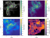Fig. 2.

Maps of the depletion time (top left), shear (top right), Mach number (bottom left), and the compressive-to-total ratio of turbulent energy (bottom right). A grayscale map of the gas density is underlaid in the top left panel and is represented as contours in the others to guide the eye. The depletion time and Mach numbers are measured at a scale of 125 pc, using stars younger than 10 Myr for the former, while the shear and compressive-to-total ratio are measured at 50 pc and their maps are density weighted histograms with a bin size of 125 pc. Small circles indicate the positions of minima of depletion times and the dashed squares show our four regions of interest. No clear correlations between these quantities are visible. This is due to the time delay between the onset of a physical trigger and the resulting star formation activity being of the same order of magnitude as the dynamical time of the merger (∼10 Myr).

We first find that, across the galaxies, t_dep has a scatter of several orders of magnitude, with sharp gradients especially around the overlap and the galactic nuclei (up to ≈20 Myr pc⁻¹), as discussed in Sect. 3.5. Other regions also host a range of depletion times. The structure of the northern arc (including our rightmost region of interest and its gaseous extension toward the top left) yields a broad distribution of depletion times and dense gas clumps not hosting star formation. The map of shear (top right panel of the figure) indicates that such clouds found at the edge of the disk remnant lie in areas of strong shear (e.g., at x ≈ 0.9 kpc, y ≈ 2.2 kpc in Fig. 2), likely caused by the differential tidal stretch that truncates the disks. Shear is thus destroying the overdensities and these structures will not survive long enough to form stars. Conversely, other clouds (farther away from the tidal truncation of the disk) are on the verge of hosting star formation in the next few Myr (e.g., at x ≈ −1.9 kpc, y ≈ 2.3 kpc).

This indicates that the large scatter of t_dep is partly due to gas structures being at different evolutionary stages, toward collapse or dissolution, and that the influence of the large-scale environment is blended with this intrinsic time sequence (see Grisdale et al. 2019 on the diversity of SFEs at cloud scale). The variations in gas depletion times are discussed further in Sect. 3.3, in relation to the distribution of dense gas.

The four panels of Fig. 2 illustrate the complexity of the picture by displaying the maps of some factors triggering or quenching star formation. In these maps, we retrieved expected general trends in most of the regions: volumes with strong shear have long depletion times, and those with strong compressive turbulence (i.e., high Mach number and high compressive-to-solenoidal ratio) tend to favor efficient star formation. Notable exceptions are the vicinity of the galactic centers, discussed in Sect. 3.5. However, a more detailed and quantitative inspection of the relations between the plotted quantities reveals no clearer trends than the general qualitative ideas mentioned above. In that sense, the causal link between these processes and star formation is not unambiguously established here, although it appears when considering the time evolution of the system (see Renaud et al. 2014, their Fig. 1).

The reason for this is likely the time delay between the onset of a physical process and the measure of the resulting star formation activity. In our case, using stars younger than 10 Myr implies that the delay is at least 10 Myr. In other words, the process that triggers (quenches) star formation as early as the formation of a cloud can be long gone when the depletion time is measured to be dropping (rising). This is particularly important in fast evolving systems like galaxy mergers where dynamical times are short. If causal relations are not found in our Eulerian scheme, they would likely get clearer by using Lagrangian methods (e.g., with tracers in grid codes, see Genel et al. 2013; Cadiou et al. 2019) and by tracking the gas material throughout the phases of compression, cooling, fragmentation, and star formation (Semenov et al. 2017).

Apparent in these maps is the diversity of environments leading to a broad dynamical range in the quantities plotted. For instance, the vicinity of the nuclei host strong shear and the depth of the potential implies fast moving gas structures, while the arc in the outskirts of the disk evolves with longer timescales. As a result, the relevant timescales for cloud evolution (and thus star formation) are strong functions of position and time, such that it is impossible to define global timescales. Therefore, observational tracers of any stage of the star formation process (from dense gas to gas-free star clusters) suffer from this diversity of timescales by likely introducing biases in the interpretation of galaxy-wide maps. For the same reason, the diversity of timescales translates into a diversity of scale-lengths which also introduce biases, as discussed in Sect. 3.4.

According to our model, the present ongoing collision is taking place ∼150 Myr after the first encounter between the galaxies, i.e., the galaxies are now falling back onto each other. The northern galaxy (NGC 4038) is moving southward toward the other progenitor. The overlap of the disks starts on the east side (left in Fig. 1) and moves roughly to the southwest as the two galaxies fly through each other. The time taken by the overlap to move from one side of the stellar disks to the other is about 10 Myr, i.e., comparable to the timescales of the physical processes mentioned above, to the depletion times of the clouds, and to the propagation time of feedback. If starbursts were exclusively triggered by shocks (when the gaseous material of the two galaxies overlap, either through cloud-cloud collisions or between the gas reservoirs of the progenitors; see Jog & Solomon 1992 and Sect. 4.2), we would expect to find a signature of this evolution with star formation running from east to west across the system. In that case, the galaxies would exhibit gradients of tracers of star formation from the signatures of the latest stages of star formation (e.g., Hα, UV, IR) toward the east, behind the shocks themselves, to more early-stage indicators (e.g., dense gas, CO, HCN, HNC) to the west. However, MUSE observations covering the entire central region reveal no such gradients in the positions or sizes of the HII regions (Weilbacher et al. 2018), indicating that shocks are not the only triggers of the starburst activity. The observed complexity is in line with our results and we predict that similar conclusions could be reached with other tracers.

In this context, using velocity dispersion only to trace star formation might lead to errors, since an above-average dispersion could be both the cause of star formation (e.g., compressive turbulence, shocks) and its consequence (feedback). Some strong shocks not associated with young stars have been detected in the Antennae (Haas et al. 2005), but exclusively in the overlap, very likely marking the onset of localized shock-triggered star formation.

Due to this diversity in star-forming regions, their triggers, and their delays, it is difficult to establish clear global relations. To circumvent this, we examine the properties of the dense ISM to identify features specific to interacting systems.

3.2. Excess of dense gas in the star-forming regions

Figure 3 shows the gas density probability distribution functions (PDFs) in our four regions and in the entire system. All PDFs yield a secondary peak of dense gas (≳10⁴ cm⁻³), but this feature is most pronounced in the nuclei and to a lesser extent in the overlap. Together, the four kpc-scale regions account for 87% of the dense gas across the galactic system. A handful of other clouds account for the remainder (on the eastern side of the northern arc, and at the southernmost end of the southern galaxy; see Fig. 1). We note that the average density of the secondary peak varies from one region to the next. Although gas less dense than this secondary peak can also form stars, the density dependence of the star formation law (∝ρ^3/2) makes the dense peak the main contributor (85%) to the total star formation activity.

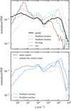Fig. 3.

Normalized mass-weighted gas density PDFs in the four regions and in the entire galaxy (top), and in the two nuclei, with and without the central clouds (i.e., the nuclei themselves; bottom). All regions exhibit a secondary peak of dense gas (≳10⁴ cm⁻³) in contrast with isolated galaxies where these highest densities only correspond to the tails of the distributions.

As shown in Fig. 3 (bottom panel) the gas clouds of the nuclei themselves (i.e., the innermost ∼100 pc) constitute a significant fraction of the mass in the secondary peak of their regions, but are not the sole contributors: the peak is still present in the PDF of the kpc-scale regions without the nuclei and its maximum is found at the same density with and without the nuclei. Star formation in the central regions is thus not solely restricted to the innermost gas structures, but spans a number of other clouds with comparably high densities, as visible in the density maps (Fig. 1). These star-forming clouds in the immediate vicinity of the nuclei could result from the fragmentation of infalling material, but the excess of dense gas and the similarities of the PDFs with and without the nuclei suggests a more efficient process.

The similarity of the PDFs across the nuclear regions, as well as the presence of the secondary peak in the overlap and arc regions, indicates that the physical origin of the second peak is a process that affects large volumes and is not solely due to nuclear inflows. Furthermore, Renaud et al. (2014, their Fig. 2) showed that the secondary peaks appear as early as the first passage in the interaction, and are thus not only limited to penetrating encounters, in line with the global increase in compressive turbulence. The link between the shape of these PDF and turbulence is further discussed in Sect. 4.1.

It is important to note that these PDFs do not result from a shift or a widening of the density distributions found in isolated galaxies: the presence of a secondary peak is unique to interactions and reflects that star formation in these systems is not a simple extrapolation of that of isolated galaxies. Therefore, the physical reason for the enhanced star formation, both in terms of rate and efficiency (i.e., SFR and t_dep), lies in the process(es) that generate this excess of dense gas. In the next section, we connect this excess to reduced depletion times.

3.3. Variations in depletion time

At the instant considered, the entire galactic system has a depletion time of 100 Myr (180 Myr, if considering the molecular and atomic gas), i.e., about one order of magnitude shorter than the depletion time of normal star-forming disk galaxies, which places it in the regime of LIRGs/ULIRGs defined by Daddi et al. (2010a).

The molecular gas depletion times for the kpc-sized overlap, nuclei and arc regions are 65, 80, and 170 Myr, respectively. Accounting for the total neutral gas reservoir (i.e., molecular and atomic gas), these depletion times increase to 120, 120, and 250 Myr, respectively. These measurements are compatible with the estimates of Bigiel et al. (2015), who reported shorter depletion times when using tracers of dense gas (∼40−160 Myr in total infrared) and longer times with CO, but on slightly larger scales (≈2−3 kpc) and by adopting disk-like luminosity-to-mass conversion factors (while the α_CO model from Renaud et al. 2018 would lead to depletion times about 1.5 shorter). By selecting the regions hosting the most intense star formation activity, we already detect significant variations in t_dep. However, these four regions are not representative of the all the star-forming ISM in the galaxies and thus we also examine the t_dep variations across the entire cloud population of the system.

The top panel of Fig. 4 shows the positions of star-forming clouds in the Schmidt–Kennicutt diagram. The surface densities are computed at the scale of each cloud (∼30 pc), independently of each others. The overall relation is super-linear as the points are best fitted by power laws of indexes 1.4 when including the two very dense clouds at the galactic centers, and 2.0 when excluding them, but with large deviations (69.2 and 19.2, respectively, in the units of the figure).

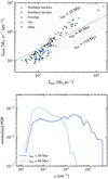Fig. 4.

Top: Schmidt–Kennicutt diagram of the clouds identified in the simulation. The two densest points correspond to the clouds at the galactic centers. The dotted lines mark constant depletion times (from 10 to 110 Myr, in steps of 10 Myr); the dark line corresponds to 40 Myr. Bottom: normalized mass-weighted gas density PDF of these clouds, split into two regimes of depletion times: < 40 and > 60 Myr. Clouds with 40 Myr < t_dep < 60 Myr correspond to the transition regime shown in the top panel and are not considered here for the sake of clarity. The distribution of clouds does not follow a unique power law, but rather a combination of two regimes: clouds with an excess of dense gas have shorter depletion times than those without.

Instead of interpreting this distribution as a unique power law with a large scatter, we highlight that a line of constant depletion time splits the clouds into two families: those with short depletion times (t_dep ≲ 40 Myr) are found at the dense end of the distribution, while the others are systematically less dense. The dichotomy directly relates to the PDFs of these clouds (see bottom panel of Fig. 4). Clouds with short t_dep systematically exhibit an excess of dense gas (≳10⁴ cm⁻³) with respect to the other clouds. More than the mere expected relation between short t_dep and high densities, this shows that all the clouds with t_dep < 40 Myr contain an excess of dense gas, while none of the others do. Furthermore, not all star-forming clouds contribute to the secondary peak noted in Fig. 3, but only those with a short t_dep, demonstrating that the excess of dense gas noted earlier as the presence of a secondary peak is associated with short depletion times, in addition to high SFRs.

On small scales, the density of star formation rate depends on the gas density in a super-linear fashion (e.g., ρ_SFR ∝ ρ^1.5 in the case of constant efficiency per free-fall time, as adopted here). This implies that, for a given gas mass, an excess of dense gas (our secondary peak) leads to a more efficient star formation (i.e., a decrease in depletion time).

Both the Schmidt–Kennicutt diagram and the distribution of t_dep show that the interacting galaxies can simultaneously contain clouds with unimodal PDFs and long depletion times (in line with those of isolated galaxies), and clouds with an excess of dense gas and significantly shorter depletion times. The mix of the two types sets the properties of the galaxies at kpc-scale, which (in our case at this instant) puts the Antennae among the galaxies with shortened depletion time in the starburst regime.

Comparable variations in t_dep have also been found observationally across the Antennae (Bigiel et al. 2015; Bemis & Wilson 2019), IC 4687 (Pereira-Santaella et al. 2016), and NGC 2276 (Tomičić et al. 2018). In the Antennae (seen in observation and in our model), the complexity of the geometry due to the deformation from the previous interaction and the partial overlap of two galaxies lead to complex galactic-scale gradients, neither radial nor from one side of the galaxy to the other (unlike in NGC 2276 where ram pressure and tides imprint clear variations in t_dep, Tomičić et al. 2018). The absence of such large-scale, smooth variations indicates that the triggers of star formation are a complex interplay of physical processes and/or of processes with timescales on the order of the dynamical times of the clouds, as suggested by Fig. 2.

The exact physical origin of this dense gas is difficult to assess in our models, as discussed in Sect. 3.1. However, some additional clues can be obtained by examining the star formation histories of the clouds. Clouds with long depletion times (t_dep > 40 Myr) are forming fewer stars now than 5 Myr ago. This indicates that their formation activity is slowing down, and will probably stop within a few Myr, due to the consumption of dense gas and/or its dispersion by feedback. The picture is less clear for the clouds with shorter t_dep. Some show an increasing star formation activity, while others behave like the longer t_dep objects mentioned previously. This points toward a mix between evolutionary and environmental effects shaping the star formation activity of these clouds (see Grisdale et al. 2019, in the context of the Milky Way.).

Interestingly, the loci of the clouds in the Schmidt–Kennicutt diagram (Fig. 4) is independent of their host region, and more generally of their position in the galaxies. In particular, we find dense clouds with short depletion times in all regions. The excess of dense gas is found during all the phases of the interaction (from the first passage to final coalescence; see Renaud et al. 2014, their Fig. 2). Although the most central clouds always exhibit the shortest depletion times, we report the existence of clouds with reduced depletion times in all regions of the galaxies during all phases of the interaction. This further establishes a link between clouds with short depletion times and the spatially extended starburst activity, and suggests that differences in the kpc-scale environment play a minor role on the properties of the clouds themselves. The other possible explanation is that the diversity of processes leading to short depletion times across the galaxies are indistinguishable in a Schmidt–Kennicutt diagram (with the exceptions of the two nuclei that reach extreme densities, but comparable depletion times to those of many other clouds).

3.4. Scale dependence

In Fig. 5, we consider different areas (or beam sizes) centered on the star formation peaks within our four regions of interest. Due to the spatially extended enhanced star formation activity, all of our regions have a depletion time an order of magnitude shorter than an equivalent volume in a normal star-forming disk (∼1 Gyr, as expected). Not surprisingly, increasing the beam size usually leads to including a larger fraction of non-star-forming gas, which increases the depletion time (see, e.g., Schruba et al. 2010). Details of this relation, however, depend on the size of individual star-forming structures and the separation between them within the beams, and the latter varies across the galaxies due to the diversity of processes involved (see Fig. 2). This is illustrated by the differences between our four regions of interest in Fig. 5, in addition to the expected general trend of increase in t_dep with the beam size, as also seen in the isolated galaxy.

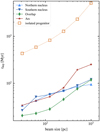Fig. 5.

Depletion times as a function of the measurement scale for our four analysis regions, and for a reference isolated progenitor galaxy. While the general trend is common to all regions, details depend on the sub-kpc structure of the ISM and significantly vary from one region to the next, due to different organizations of the clouds set by the kpc-scale environment.

For instance, star formation in the arc occurs in a handful of clouds, surrounded by non-star-forming diffuse material. Therefore, the depletion time in this area rapidly increases when it is measured on scales larger than the size of these clouds. In the other regions, this effect is still visible but without a particular scale identifiable due to the larger filling factor of clouds in the area³, which means that increasing the beam size leads to including more clouds, i.e., a smaller fraction of non-star-forming material than in the arc.

Figure 6 shows the distribution of depletion times when measured on cloud (30 pc) and galactic (500 pc) scales. On large scales, the regions of shortest depletion times are blended with little or no star-forming material, which truncates the distribution on the short t_dep side. For the same reason, regions not forming stars (t_dep = ∞) are binned with regions with long (but finite) depletion times (≳5 Gyr), which extends the distribution to its long side with respect to that on small scales. As expected, using beam sizes larger than star-forming regions dilutes them toward longer t_dep.

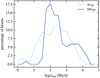Fig. 6.

Distribution of depletion times, measured in 30 pc and 500 pc beams on a Cartesian grid (with arbitrary origin, i.e., not centered on peaks of star formation) in the central 6 kpc × 6 kpc of the system. For better statistics, we repeat the measurements by shifting the origin of the grid by several fractions of the beam size, and stack the distributions obtained. Large-scale measurements have a bimodal distribution of short (∼100 Myr) and long (∼2 Gyr) t_dep.

The galactic-scale distribution reveals the two modes of depletion times: the main one at ∼100 Myr and a secondary at ∼2 Gyr. These average t_dep values approximately correspond to those of the disk and starburst regimes found in Schmidt–Kennicutt diagrams (e.g., Daddi et al. 2010a; Genzel et al. 2010). On the cloud scale, however, the distribution is narrower (although it appears wider due to the log-scale of Fig. 6) because of the lack of the dilution effect mentioned above. However, it still spans several orders of magnitude in depletion times, despite the uniform star formation recipe at constant SFE imposed (0.02 at 1.5 pc). Details of the physical origin of this scatter are discussed in Grisdale et al. (2019) in the context of more quiescent disk galaxies, and Kraljic et al. (in prep.) in the case of interacting systems.

In summary, all regions contain clouds with short and long depletion times, with an excess of dense gas or not. This implies that the galactic-scale dynamics has either no influence on the depletion times of individual clouds, and thus that the scatter is a purely intrinsic evolution, or that the different dynamical triggers at stake have the same signatures on the depletion times. However, the details in the scale dependence of t_dep reveal a different organization of the star-forming material from one region to the next (in particular in the arc) linked with the kpc-scale triggering of cloud formation.

3.5. Long depletion times in the nuclei

Figure 5 shows that the depletion time yields a steeper dependence with scale for beam sizes ≲100 pc in the nuclei than in the overlap and the arc. The reason for this originates from the peculiarity of the nuclei in the gravitational potential of the galaxies. Being natural convergence points of flows and minima in the potential, they induce strong shearing and tidal effects along the fueling channels toward them (see Fig. 2). These effects smooth out most (but not all) of the gas clumps, and in turn prevent their collapse on overdense seeds. Consequently, and despite large amounts of dense gas, star formation is considerably slowed down a few 100 pc away from the centers. However, when the gas reaches the nuclei themselves (∼50−100 pc in our simulation) it accumulates, leading to important overdensities and the observed star formation activity. As a result, efficient star formation is concentrated in the main structure of the nuclei, while it is more evenly distributed in the overlap, due to the large shocked and compressed volumes. This situation is qualitatively comparable to that of barred galaxies where the bar(s) generate the torques necessary to fuel large amounts of gas, but where shear increases t_dep of this gas, or even quenches star formation (see Emsellem et al. 2015; Renaud et al. 2015b, in the context of the Milky Way), with the notable difference that the excess of dense gas in the Antennae allows some clouds to survive destruction, due to their higher binding energy (see Figs. 1 and 2, and Sect. 4.2).

This point explains why observations focusing on the nuclei can report longer depletion times there than in the overlap, despite higher SFRs (see, e.g., Bigiel et al. 2015). Our results predict that observing these regions with beams comparable to the sizes of the star-forming area only (i.e., encapsulating as little surrounding non-star-forming material as possible) would lead to the expected shorter t_dep in the nuclei. We also note that the scale dependence of the depletion time varies with the clumpy nature of star formation, which itself depends on the tracer used to measure the SFR. For instance, a tracer of molecular gas is expected to reflect larger objects and thus milder variation in t_dep with the scale than, for example, the Hα luminosity which is more concentrated around the star-forming sites.

3.6. CO emission

3.6.1. Spectral line energy distributions

Figure 7 shows the spectral line energy distributions (SLEDs), in term of integrated intensity and flux integral, of our regions (1 kpc) compared to entire galaxies (10−30 kpc): the Antennae at the same time (labeled “global”), at the time of maximum starburst (labeled “ULIRG”), a Milky Way-like galaxy, and a high-redshift clumpy disk.

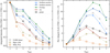Fig. 7.

CO spectral line energy distributions for velocity-integrated brightness temperature (left) and velocity-integrated flux density (right), both normalized to CO(1–0), in our four selected regions (filled symbols), in the entire system (global), in the same simulation but during the starburst episode (ULIRG), in a gas-rich clumpy disk (high-redshift), and in a Milky Way-like galaxy (open symbols). The SLEDs of the most actively star-forming regions (nuclei and overlap) resemble that of the Antennae (global and ULIRG), while the arc better matches the high-redshift disk at high J_upper.

Our regions of interest encompass a range of densities, from the peaks in the clouds to the more diffuse warm medium between them. For this reason, we expect our modeled CO emission to differ from that observed when exclusively focusing on clouds. Our results would thus better match observations with beams not resolving the individual clouds and thus blending the peaks of cold emission with warmer media, i.e., on scales on the order of and larger than ∼1 kpc. While our results for the Antennae are indeed in qualitative agreement with the observations of Bigiel et al. (2015, ∼0.6 kpc beams, centered on peaks), they better match those of Schirm et al. (2014, ∼4 kpc beams), as discussed in Appendix A. All four of our regions and the Antennae system (global and ULIRG in Fig. 7) yield a strong CO(3–2) emission, scattered around CO(3−2)/CO(1−0) ≈ 0.6, which is similar to the expected values in (U)LIRGs (Yao et al. 2003; Papadopoulos et al. 2012; Bolatto et al. 2015).

The high CO(3–2) intensity (in particular the ratio of brightness temperatures CO(3–2)/CO(2–1)) in the kpc-scale regions is not retrieved in any of the large-scale measurements, regardless of the star formation activity. A similar trend might be seen in the observational SLEDs from Bigiel et al. (2015) who used a beam size smaller than our regions (≈0.6 kpc). This suggests that this emission is localized in small volume(s), and thus gets blended with regions of weaker emission on larger scales. This may correspond to the CO(3–2) detection in the real system of a bright super giant molecular cloud (known as the firecracker) supposedly being the future formation site of a massive star cluster (Whitmore et al. 2014, see also Johnson et al. 2015).

At higher excitation levels (J_upper ≥ 4−5), the nuclei and the overlap regions have SLEDs comparable to that of the ULIRG phase, but the arc (and the galactic-scale global measurement) more closely resembles a high-redshift clumpy galaxy, with a significant bend in their SLEDs (in integral intensity). We propose an interpretation of these features in Sect. 4.3.

Figure 8 shows the contribution of the regions (1 kpc scale) to the global CO(J → J − 1) intensity (10 kpc scale). As expected, each region contributes more than average to the global intensity, for all transitions. Their combined contribution ranges from ≈40% (CO(1–0)) to 75% (CO(6–5)) of the total intensity, and 85% of the SFR, although they only span 4% of the area considered. The remaining, yet significant, fraction of the flux originates from less concentrated regions.

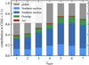Fig. 8.

Contribution to the CO(J→J-1) line from our four 1 kpc × 1 kpc regions, with respect to the entire system (global, i.e., 10 kpc × 10 kpc). The relative contribution of our four regions varies with J_upper due to differences in the density, temperature, and velocity dispersion of the ISM, particularly in the inter-cloud medium.

The relative contribution of the individual regions increases with J_upper up to 6 for the nuclei and the overlap. However, that of the arc peaks at CO(4–3), which further distinguishes the arc. As shown in Figs. 7 and 8, the southern nucleus is more excited and has a higher CO intensity than the northern nucleus at all J_upper, despite hosting lower amounts of dense gas and with lower maximum densities (Fig. 3), and a comparable distribution of temperatures. One would then expect a stronger emission from the northern nucleus, in contrast to our measurements; however, it hosts a stronger shear and higher Mach number (Fig. 2) than its southern counterpart, i.e., an overall larger gas velocity dispersion, which accounts for a stronger absorption of the CO flux captured by the LVG method. The exact relative roles of the gas density, the temperature, and the velocity dispersion are difficult to assess due to sharp variations in these quantities on small scales and the limited resolution of our analysis. Our results on the differences between the regions presented in the previous sections highlight that the relative importance of each quantity varies across the galaxy (and thus likely in time as well) in a complex manner (see also Sect. 4.3).

3.6.2. Spatial variations of α_CO

Figure 9 shows the CO-to-molecular conversion factor α_CO in our regions. As noted in Renaud et al. (2019), the SFR and its surface density are not good tracers of variations in α_CO, and the recent SFH must also be considered, in particular to account for the effects of feedback on temperature and velocity dispersion. When doing so, we find that all regions contain stars formed during the first passage (≈150 Myr), and a recent boost of the activity (≈20 Myr) due to the second encounter. By tracking backward in time, we find that the material in the present-day arc region comes exclusively from the outer disk, while the overlap comprises material from a wider range of radii, including only several kpc from the galactic centers. The difference in gas densities between these volumes explains that, during the separation of the galaxies, star formation slows down significantly more in the future arc material than in the elements ending up in the other regions. This translates into a deficit of 20−100 Myr old stars in the arc compared to the other regions. Furthermore, tides, shear, shocks, and the resulting turbulence reshape the structures of clouds, particularly in the nuclei and the overlap, which shifts young stars away from the densest gas. As a result, stellar feedback can propagate further and with less resistance to large scales in the nuclei and the overlap (see Sect. 4.4). Therefore, the ISM of the nuclei and the overlap contain more gas of intermediate densities and warm temperatures (∼10 cm⁻³, 10⁴ K) than the arc. The media in which CO emission propagates are thus different in the arc and the other regions, which translates into a different absorption and in turn, into a different α_CO. The same argument explains the slight difference between the two nuclei (see also Sect. 3.6.1).

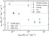Fig. 9.

The α_CO factor as a function of the surface density of SFR in the four selected regions (1 kpc × 1 kpc, filled symbols), for the entire merger system (global), the same system during the ULIRG phase, a gas-rich clumpy disk (high-redshift) and a Milky Way-like galaxy (open symbols). The error bars show the dispersions of the values, evaluated by varying the line of sight (see Sect. 2.2). Horizontal lines indicate the values commonly used in observations (4.3 for disks, Bolatto et al. 2013, and 0.8 for ULIRGs, Downes & Solomon 1998). Important variations in α_CO are found across the galaxies, due to different interplays of physical processes setting the assembly of star-forming regions, and making our regions lie in between the values traditionally assumed for disks and ULIRGs.

The new onset of star formation triggered by the second passage (∼5 Myr ago) is too recent to have significantly altered the CO emission and propagation over kpc scales (see Renaud et al. 2019), and therefore only the older activity affects our results. The galaxies thus lie on the post-burst regime and with slightly higher α_CO values in the outskirts of the disks than in the central regions. These spatial variations are comparable to the observations of Sandstrom et al. (2013) who report a depression of α_CO by a factor of about two in the centers of their isolated galaxies (see also Strong et al. 2004), but otherwise flat gradients across the disks. They invoke a possible contribution from diffuse medium in lowering the α_CO factor (Liszt et al. 2010; Liszt & Pety 2012), but the physical reason is probably different in our case, and might be due to differences in the ISM structure between their isolated disks and our interacting system. Sandstrom et al. (2013) also note that the interacting case in their sample (M 66) exhibits more uniform values of α_CO across its disk, but this particular galaxy is only mildly interacting with its neighbors with little perturbation of its structure, in contrast with our starbursting case. Therefore, the spatial variations of ISM properties and α_CO might not be directly comparable between our studies.

Our simulations show that globally α_CO is significantly smaller in interacting systems than in isolated galaxies, independently of the gas fraction (or equivalently redshift; see also Bournaud et al. 2015; Renaud et al. 2019). This is consistent with the observations of Tacconi et al. (2008) who argue for α_CO ≈ 1.0−2.4 in submillimeter galaxies (z ∼ 2 and Σ_SFR ∼ 10−100 M_⊙ yr⁻¹ kpc⁻²), which also exhibit high SFRs and short depletion times (Greve et al. 2005; Bouché et al. 2007; Magnelli et al. 2012), as opposed to high-redshift isolated disks for which α_CO is closer to the Milky Way value. This confirms that regions with a high Σ_SFR can have either a high or a low α_CO, but those with short depletion times correspond to low values of α_CO.

As noted in Renaud et al. (2019), the value of α_CO for the entire system ranges from 4.27 in the isolated phase to 1.78 at the peak of the starburst triggered by the final coalescence, i.e., a variation of a factor of 2.4 during the merger. This is comparable to the variation between our regions of interest from our selected snapshot (from 1.3 to 2.8, i.e., a factor of 2.2; see Fig. 9). However, it should be noted that we focus our analysis on actively star-forming regions, and that α_CO is likely much higher in other areas. Therefore, we expect the spatial variations of α_CO to be larger than temporal variations, even for a system that passes from the normal disk to the starburst regime. This could have important implications for the interpretation of observations resolving the diversity of star-forming environments, even across a given galaxy.

4. Discussion

4.1. Compressive turbulence and the shape of the density PDF

Sub-kpc scale simulations of the ISM are commonly used to study the inner physics of molecular clouds, down to the individual star level (see Hennebelle & Falgarone 2012, for a review). These simulations do not include the galactic scales from which part of the turbulence is generated (≳0.1−1 kpc; see Agertz et al. 2009; Bournaud et al. 2010; Renaud et al. 2013; Falceta-Gonçalves et al. 2015; Grisdale et al. 2017), and they must resort to manually forced turbulence. Such works indicate that the turbulent ISM yields a log-normal density PDF (see, e.g., Vazquez-Semadeni 1994) for which the variance may be written

$\begin{matrix} σ^{2} = ln (1 + b^{2} M^{2}), \end{matrix}$ $\begin{aligned} \sigma ^2 = \ln {\left(1+b^2{{\mathcal{M} }}^2\right)}, \end{aligned}$ (1)

where ℳ is the Mach number, and b is a dimensionless parameter related to the forcing nature of the turbulence, i.e., the mix between its compressive (i.e., curl-free) and solenoidal (i.e., divergence-free) modes (see, e.g., Kritsuk et al. 2007; Federrath et al. 2010). In these simulations, the PDF is found to always have a log-normal shape⁴, regardless of the turbulence forcing (with a power-law tail at high densities when self-gravity is captured; Ballesteros-Paredes et al. 2011; Elmegreen 2011; Renaud et al. 2013). In other words, for a given Mach number these simulations yield a wider but still log-normal PDF in compressive turbulence than for equipartition.

As presented in Renaud et al. (2014) and Fig. 3, the shape of the density PDF in our interacting galaxy models, which show the formation of a secondary peak at high densities, significantly deviates from the classical log-normal shape during the interactions (see also Teyssier et al. 2010; Bournaud et al. 2011). The same bimodal feature is also seen in real interacting galaxies in terms of line-width distributions (Sun et al. 2018), further suggesting the superposition of a high σ mode on the classical mode in efficiently star-forming systems. Renaud et al. (2014) attributed this excess of dense gas to turbulent compression that arises during the interaction: changing the turbulence from energy equipartition between the compressive and solenoidal modes before the interaction to a compressive-dominated turbulence until the post-merger phase increases the gas density contrast and generates this excess of dense gas. Therefore, a discrepancy exists between the log-normal PDF from forced compressive turbulence in small-scale simulations, and the double-peaked PDF measured in the compressive turbulence of galaxy mergers (as is, i.e., without any manual forcing).

In the context of the Schmidt–Kennicutt relations, the analytical model of Renaud et al. (2012) uses the secondary peak to explain the observed differences in depletion times between disks and starbursting galaxies. In this model (and others of the same nature, see, e.g., Padoan & Nordlund 2011; Hennebelle & Chabrier 2011; Federrath & Klessen 2012), using a log-normal PDF shape for all galaxies would lead to a unimodal star formation law, in which the SFR is set by the width of the PDF (Eq. (1)), and would thus not retrieve the difference between a gas-rich isolated disk with a high SFR (e.g., BzK galaxies, Daddi et al. 2010b) and a local (U)LIRG with the same SFR (Kennicutt 1998). In other words, increasing the variance of the log-normal PDF (either by increasing ℳ or b in Eq. (1)) would only shift a galaxy along the canonical Schmidt–Kennicutt relation, while keeping it on the relation. Such a model could retrieve a diversity of SFRs, but not the diversity of depletion times. Another effect is needed to change the regime, for example moving from the relation of disks to that of starbursts by decreasing the depletion time.

As discussed in Sect. 3.3, the super-linearity of the star formation law linking the local density of SFR to that of gas is the key to changing the regime, i.e., to moving the galaxy from the relation of disks to that of starbursts. With a wide, unimodal PDF the densest gas constitutes the tail of the PDF, and increasing its width leads to a higher SFR. Conversely, the presence of a secondary peak in the distribution (i.e., the excess of dense gas we report) and the super-linearity of the star formation law imply that most of the star formation activity takes place at the highest densities, therefore with a higher efficiency than usual (i.e., a shorter depletion time). (See Renaud et al. 2012 for an analytical demonstration, and see also Fig. 4.)

We thus report a fundamentally different shape of the PDF between that from manual forcing of compressive turbulence in sub-kpc scale simulations and that of compressive turbulence consistently arising in our simulations of interacting systems. We do not fully understand the reason of this difference, but assuming it originates from the different setups of the simulations, we postulate it could be related to the injection scale of the turbulence, its forcing mechanism, and/or its dissipation. It could also be that galactic simulations contain large gas reservoirs to replenish the PDF when compression occurs, while simulations at cloud scales would suffer from a rarefaction of gas to populate both of our peaks. By nature, galactic scale simulations like ours are likely better at capturing the injection and forcing mechanisms, but the limited resolution implies the dissipation is less accurate than in small-scale studies. Further investigations with a large dynamical range are needed before we can draw firm conclusions.

The exact nature of turbulence has important implications for the structure of the ISM and the propagation of feedback, potentially down to the stellar initial mass function (IMF) itself. For instance, theoretical models predict that a compressive turbulence would lead to a bottom-heavy IMF (Chabrier et al. 2014). However, Renaud et al. (2014) have established the existence of compression-dominated turbulence in interactions only at the scale of ∼40 pc, i.e., several orders of magnitude larger than that of pre-stellar cores. Therefore, there are still many uncertainties on how this type of turbulence, driven by galactic dynamics, cascades and potentially dissipates down to the core scale, in addition to our lack of understanding of the core-to-star mapping (Goodwin et al. 2008; Motte et al. 2018). Small-scale studies with detailed implementations of a range of physical processes conclude that the IMF is independent of environmental conditions, and in particular does not vary with turbulent properties of the gas or the metallicity (Bate 2009, 2019; Myers et al. 2011). However, including self-consistently the full range of galactic-driven effects, in particular turbulence injected at ≳100 pc scale, seems essential to capture and predict the possible variations in the IMF. This is still beyond the reach of present-day models and supercomputing resources.

4.2. The galactic nuclei as collision environments

All the aspects of our analysis reveal similarities between the overlap and the nuclei, suggesting that the former could be a scaled-down version of the latter, i.e., with similar physical processes active, but at lower rates. From a morphological point of view, the two types of regions show several dense, cold star-forming clumps, with an average separation of ≈130 pc, distributed along elongated structures of warm gas at intermediate densities (∼10²⁻³ cm⁻³, ∼10¹⁻² K), themselves surrounded by more diffuse medium (∼1−10 cm⁻³, ∼10²⁻⁴ K).

The overlap is, by definition, the location of kpc-scale shocks between the gas reservoirs and the clouds (and/or marginally stable overdensities) they contain (Jog & Solomon 1992). As simulated and observed in other contexts, cloud-cloud collisions trigger star formation (Tan 2000; Tasker & Tan 2009; Inoue & Fukui 2013) in the form of massive clusters (due to the enhanced external pressure Elmegreen & Efremov 1997; Fukui et al. 2014) and possibly massive stars (Motte et al. 2014; Takahira et al. 2014). Although it is difficult in our Eulerian simulation to track individual gas structures and establish collision rates, the presence of thin and dense tidal tails and bridges connecting the density peaks in the overlap confirms the ubiquity of cloud-cloud collisions (Fig. 1). It is thus likely that a significant fraction of the star formation activity in the overlap is linked to cloud-cloud or cloud-reservoir collisions.

In the nuclei, the gas is fueled toward the center by negative gravitational torques, mainly from one galaxy on the other (Keel et al. 1985; Hernquist & Katz 1989; Barnes & Hernquist 1991), but also from asymmetric structures (see, e.g., Emsellem et al. 2015). The clumpy nature of the fueled material (see Sect. 3.5) makes the nuclear accretion comparable to a series of cloud-cloud collisions. In that sense, the nuclei share a common mechanism with clouds in the overlap region, but likely at a higher rate due to their preferential location in the potential.

In both the overlap and the nuclei, the trigger(s) of star formation is a short-range effect whose intensity peaks during penetrating galaxy encounters (but remains relatively high during separation phases, due to the high gas density in these inner galactic regions), which then explains that the α_CO values of these areas are closer to the starburst regime highlighted in Renaud et al. (2019) than to the transitional post-burst regime as it is clearer for the arc.

In short, the nuclear inflows induced by gravitational torques during close encounters play a similar role as the overlap of the outer disks, by triggering collisions between dense gas structures that lead to a starburst activity lasting ∼100 Myr (Renaud et al. 2014). The similar physical processes translate into SLEDs and α_CO factors in the galactic nuclei and the overlap resembling those of starbursting systems, while the activity in the arc appears to have fundamentally different signatures, closer to that of disks with a high but steady SFR.

4.3. Imprint of the ISM structure on the CO emission

By separately fitting the SLEDs from the cold and warm phases, Schirm et al. (2014) established a transition at J_upper ≈ 4−5, with the emission from the cold phase dominating the small J_upper regime. All our regions share a comparable distribution of cold ISM (≲100 K) and have similar SLEDs at small J_upper (Fig. 7), which confirms the conclusion of Schirm et al. (2014).

In this regime, the behavior of our SLEDs corresponds to a ULIRG (or starburst) type of activity (as opposed to a disk, steady regime of star formation). However, at higher J_upper, the arc deviates from the common ULIRG-like behavior and more closely resembles a high-redshift disk. This is due to a different inter-cloud medium in the arc where the dense gas is highly concentrated into clouds surrounded by relatively diffuse medium (∼10 cm⁻³, see Fig. 3), like the massive clumps in high-redshift gas-rich disks (see discussion in Bournaud et al. 2015). Conversely, due to destroying tides, shear, and the overall smaller separation between the star-forming regions (Sect. 3.4), the inter-cloud media of the nuclei and the overlap gather larger amounts of dense and warm gas (∼10²⁻³ cm⁻³, 10⁴ K), likely heated by stellar feedback which propagates farther from the young stars in such inhomogeneous, porous media (see Ohlin et al. 2019, and the next section). Because these types of regions typically dominate the emission of (U)LIRGs (Fig. 8), they are good representatives of our large-scale SLEDs (labeled global and ULIRG in Fig. 7).

The state of the medium surrounding the density peaks is critical in order to set the external pressure on the clouds, and it possibly sets the mass of the star clusters formed (Elmegreen & Efremov 1997; Ashman & Zepf 2001; Maji et al. 2017). Although our model predicts comparable pressures for the overlap and the nuclei (as estimated observationally by Schirm et al. 2014), a comparison of the mass of the clusters is likely inadequate when considering the extreme cases of nuclear clusters. However, our analysis also leads (at first order) to a higher pressure in the overlap than in the arc, which would translate into more massive clusters in the former region. Even so, comparable massive clusters are found in both regions in our simulation (Renaud et al. 2015a) and in the observations (e.g., Bastian et al. 2009), which calls into question the sole role of pressure in setting the mass of young clusters.

4.4. The importance of capturing the structure of the cold ISM

Our results on the CO emission and the diversity of depletion times reflect the distribution of dense gas, and also the nature of the surrounding, more diffuse ISM. The hierarchical nature of the ISM (Elmegreen & Efremov 1997; Elmegreen 2008) is crucial here in order to assess how star-forming seeds are fueled with gas, and how fluxes are emitted and absorbed. For instance, as we noted above, the decoupling of the stars from their gas nursery, mainly due to the dissipative nature of the ISM (Renaud et al. 2013) or because of deformation of the clouds by tides or shear, can lead to significant drifts of young stars away from the densest regions of the clouds. In this context, the porosity of the ISM is equally important, particularly to regulate the propagation of feedback effects. This porosity is not only set by the level of turbulence (i.e., the Mach number), but also by the nature of turbulence (compressive versus solenoidal). While a solenoidal-dominated turbulence tends to homogenize the ISM by smoothing out density contrasts (and thus slowing down or even quenching star formation), a compressive-dominated turbulence favors the formation of high-density filaments and clumps, surrounded by low-density cavities and chimneys. These low-density volumes then facilitate the propagation of feedback effects (ionization, energy, momentum, chemical enrichment) to large distances, but along preferred directions of least-resistance, as demonstrated by Ohlin et al. (2019). It is thus likely that the regulation of star formation by feedback effects is also a function of the nature of turbulence, and thus (following the results presented here) the depletion time of the cloud itself.

To conclude, turbulence has multiple roles: by setting the distribution of dense gas (at ∼10−100 pc scale), it shapes the formation of the star-forming clouds (which can then fragment and gravitationally collapse; Vázquez-Semadeni et al. 2009), it makes the low-density channels in which the propagation of feedback is facilitated, and it sets the optical depth through a series of high- and low-density structures. It is therefore of prime importance for models and simulations to capture the turbulence and its potential diversity over a wide dynamical range.

5. Conclusions

We presented an analysis of the spatial variations of the star formation activity in a numerical model of Antennae-like interacting galaxies at parsec resolution. We identified several mechanisms that enhance or slow down star formation, and study their interplay and observable signatures in different regions of the galaxies. Our main conclusions are as follows.

The interplay of the physical processes acting on star formation exhibits complex variations in space. Their timescales are comparable to those of the dynamics of interacting galaxies (i.e., a few 10 Myr), implying that the initial cause(s) of the formation (or destruction) of clouds can be long gone when star formation itself occurs. As a result, no clear (anti-)correlation can be found between the causes (inflows, shocks, tidal and turbulent compression, shear, tidal stress) and the consequences of star formation. These correlations are, however, unambiguous when integrating over galactic scales and examining the time-evolution along the interaction and the merger (Renaud et al. 2014).
All star-forming clouds yield enhanced SFRs and reduced depletion times with respect to isolated galaxies. On cloud-scales, a correlation exists between short depletion times (≲40 Myr) and excess of dense gas visible as a secondary peak in the density PDF (≳10⁴ cm⁻³). This occurs in all regions of the galaxies, with no apparent dependence on space (i.e., no gradient or symmetries). This translates on galactic scales into the entire system moving from the canonical Schmidt–Kennicutt relation of star-forming disks to the regime of starbursts, i.e., with depletion times reduced by a factor of ≈10.
While all clouds have comparable sizes (radii of ∼30 pc at their 50 cm⁻³ contour), the diversity of processes acting on the assembly and destruction of gaseous overdensities leads to different separations between the clouds in different regions of the galaxies (120−270 pc). This has an imprint on the scale-dependence of measurements of the star formation activity such as the depletion time.
The differences in the kpc-scale ISM between the arc and the other regions is visible in the CO emission, at high J transitions. This is likely due to an excess of warm gas in the other regions, originating from the efficient propagation of stellar feedback in the inter-cloud medium (∼10 cm⁻³). It follows that the arc shows CO SLEDs comparable to those of isolated disks (at low and high redshifts). The other regions contribute in larger proportions to the global emission of the system, and thus imprint the CO emission of (U)LRIG-like galaxies.
We report significant spatial variations of the α_CO factor across the galaxies, at least as important as the time variations along the course of the interaction, i.e., between the isolated progenitor phase and the peak of starburst.
The excess of dense gas correlates with the onset of a compression-dominated turbulence, but the shape of the PDF fundamentally differs from that measured in simulations of isolated clouds. The reasons for this discrepancy are still under investigation.

Although the links between the physical processes and their observational signatures are highly degenerated, combining different tracers and indicators of the amounts and distributions of dense gas (e.g., CO, HCN, HNC), its excitation (velocity dispersion, SLEDs including both low and high transitions), and the star formation activity (its rate and efficiency) would help in disentangling comparable physical conditions. This could be particularly useful when individual star-forming regions cannot be resolved, for example in high-redshift galaxies. For instance, at a given surface density of gas, a short depletion time traces an excess of dense gas, which calls for a kpc-scale trigger. In such a medium, an highly excited CO at J_upper ≳ 4−5 likely corresponds to shocks (or equivalently to an infall toward a unique convergence point). However, a more moderate SLED would indicate compression from larger scales, possibly of tidal and turbulent origin (like in the arc in our study). How these different states are combined and mix across the galaxy could then help infer the underlying nature of the galaxy and its evolutionary stage in the case of an interacting system. It would also provide constraints on the value of α_CO to be adopted (see also Renaud et al. 2019). We note, however, that such a diversity of mechanisms comes with a diversity of timescales, which can be of the same order as the dynamical time of galaxies, especially in quickly evolving systems (e.g., interactions, bars, galactic centers). This blurs the identification of the physical processes at stake in a complex manner, which further calls for the use of as many independent tracers as are available.

The identification of the physical trigger of the star formation enhancement in interacting galaxies is a difficult task, even in simulations. Our analysis reveals resemblances between the overlap and the two nuclei, with a comparable influence of shocks between the gas reservoirs and cloud-cloud collisions. This is balanced by a strong shear on the infalling material at the vicinity of the nuclei. In this respect, the arc stands out as it hosts no cloud-cloud collisions, no shocks, and no inflows. The only physical process left to explain the enhancement of star formation (high SFR and short depletion time) is tidal and turbulence compression (Renaud et al. 2014). We note that clouds formed there are less numerous than in other regions, but once formed they have comparable properties (sizes, mass, PDF, depletion times) to those in the most active regions. The similarities at 1−30 pc scales are also seen in the formation of massive star clusters (Renaud et al. 2015a). The main difference we found is for the CO emission from the warm phase of the ISM (∼10⁴ K, J_upper ≳ 4−5). The key to determining observationally the physical trigger of enhanced star formation could thus be hidden in the medium surrounding the clouds themselves.

¹

Not to be confused with the dimensionless small-scale star formation efficiency (SFE) describing the stellar mass produced from a given amount of gas, typically at subcloud scales (≲1 pc) and often implemented in subgrid recipes of star formation. For the sake of clarity, we do not use the term “efficiency” to describe the galactic-scale quantity, but rather use depletion time, which is its direct inverse. The small-scale SFE and the galactic-scale depletion time are not directly related (see Semenov et al. 2018).

²

Therefore, only the regions having hosted star formation in the last 10 Myr appear on this map. A larger age cut would provide better statistics, but would also encompass stars that might have significantly drifted away from the locations (and thus the physical conditions) of their formation.

³

The mean separation between clouds is 270 pc in the arc and 120−140 pc in the other regions. The clouds have different shapes (e.g., some are elongated due to shear), but their volume is approximately constant across the galaxy, corresponding to spheres of radius 30−35 pc.

⁴

A log-normal density PDF may arise artificially from observations due to incompleteness of the lowest column density bins truncated by a limited field of view (Alves et al. 2017). The log-normal shape is retrieved, however, when considering large enough areas to encompass the low-density envelops of clouds in closed contours (Körtgen et al. 2019).

Acknowledgments

We thank the referee for a constructive report. FR and OA acknowledge support from the Knut and Alice Wallenberg Foundation. OA acknowledges support from the Swedish Research Council (grant 2014-5791). AH was supported by the Programme National Cosmology et Galaxies (PNCG) of CNRS/INSU with INP and IN2P3, co-funded by CEA and CNES, and by the Programme National Physique et Chimie du Milieu Interstellaire (PCMI) of CNRS/INSU with INC/INP, co-funded by CEA and CNES. This work was supported by GENCI (allocations A0030402192 and A0050402192) and PRACE (allocation pr86di) resources.

References

Agertz, O., Lake, G., Teyssier, R., et al. 2009, MNRAS, 392, 294 [NASA ADS] [CrossRef] [Google Scholar]
Agertz, O., Kravtsov, A. V., Leitner, S. N., & Gnedin, N. Y. 2013, ApJ, 770, 25 [NASA ADS] [CrossRef] [Google Scholar]
Alves, J., Lombardi, M., & Lada, C. J. 2017, A&A, 606, L2 [NASA ADS] [CrossRef] [EDP Sciences] [Google Scholar]
Ashman, K. M., & Zepf, S. E. 2001, AJ, 122, 1888 [NASA ADS] [CrossRef] [Google Scholar]
Ballesteros-Paredes, J., Hartmann, L. W., Vázquez- Semadeni, E., Heitsch, F., & Zamora- Avilés, M. A. 2011, MNRAS, 411, 65 [NASA ADS] [CrossRef] [Google Scholar]
Barnes, J. E. 2004, MNRAS, 350, 798 [NASA ADS] [CrossRef] [Google Scholar]
Barnes, J. E., & Hernquist, L. E. 1991, ApJ, 370, L65 [NASA ADS] [CrossRef] [Google Scholar]
Bastian, N., Trancho, G., Konstantopoulos, I. S., & Miller, B. W. 2009, ApJ, 701, 607 [NASA ADS] [CrossRef] [Google Scholar]
Bate, M. R. 2009, MNRAS, 397, 232 [NASA ADS] [CrossRef] [Google Scholar]
Bate, M. R. 2019, MNRAS, 484, 2341 [NASA ADS] [CrossRef] [Google Scholar]
Bemis, A., & Wilson, C. D. 2019, AJ, 157, 131 [NASA ADS] [CrossRef] [Google Scholar]
Bigiel, F., Leroy, A., Walter, F., et al. 2010, AJ, 140, 1194 [NASA ADS] [CrossRef] [Google Scholar]
Bigiel, F., Leroy, A. K., Blitz, L., et al. 2015, ApJ, 815, 103 [NASA ADS] [CrossRef] [Google Scholar]
Bolatto, A. D., Wolfire, M., & Leroy, A. K. 2013, ARA&A, 51, 207 [Google Scholar]
Bolatto, A. D., Warren, S. R., Leroy, A. K., et al. 2015, ApJ, 809, 175 [NASA ADS] [CrossRef] [Google Scholar]
Bouché, N., Cresci, G., Davies, R., et al. 2007, ApJ, 671, 303 [NASA ADS] [CrossRef] [Google Scholar]
Bournaud, F., Elmegreen, B. G., Teyssier, R., Block, D. L., & Puerari, I. 2010, MNRAS, 409, 1088 [NASA ADS] [CrossRef] [Google Scholar]
Bournaud, F., Chapon, D., Teyssier, R., et al. 2011, ApJ, 730, 4 [NASA ADS] [CrossRef] [Google Scholar]
Bournaud, F., Daddi, E., Weiß, A., et al. 2015, A&A, 575, A56 [NASA ADS] [CrossRef] [EDP Sciences] [Google Scholar]
Brandl, B. R., Snijders, L., den Brok, M., et al. 2009, ApJ, 699, 1982 [NASA ADS] [CrossRef] [Google Scholar]
Cadiou, C., Dubois, Y., & Pichon, C. 2019, A&A, 621, A96 [NASA ADS] [CrossRef] [EDP Sciences] [Google Scholar]
Casasola, V., Bettoni, D., & Galletta, G. 2004, A&A, 422, 941 [NASA ADS] [CrossRef] [EDP Sciences] [Google Scholar]
Chabrier, G., Hennebelle, P., & Charlot, S. 2014, ApJ, 796, 75 [NASA ADS] [CrossRef] [Google Scholar]
Chien, L.-H., & Barnes, J. E. 2010, MNRAS, 407, 43 [NASA ADS] [CrossRef] [MathSciNet] [Google Scholar]
Combes, F., Prugniel, P., Rampazzo, R., & Sulentic, J. W. 1994, A&A, 281, 725 [NASA ADS] [Google Scholar]
Cullen, H., Alexander, P., & Clemens, M. 2006, MNRAS, 366, 49 [Google Scholar]
Daddi, E., Elbaz, D., Walter, F., et al. 2010a, ApJ, 714, L118 [Google Scholar]
Daddi, E., Bournaud, F., Walter, F., et al. 2010b, ApJ, 713, 686 [NASA ADS] [CrossRef] [Google Scholar]
Dale, J. E., Ercolano, B., & Bonnell, I. A. 2012, MNRAS, 424, 377 [NASA ADS] [CrossRef] [Google Scholar]
Downes, D., & Solomon, P. M. 1998, ApJ, 507, 615 [NASA ADS] [CrossRef] [Google Scholar]
Dubois, Y., & Teyssier, R. 2008, A&A, 477, 79 [NASA ADS] [CrossRef] [EDP Sciences] [Google Scholar]
Eisenstein, D. J., & Hut, P. 1998, ApJ, 498, 137 [NASA ADS] [CrossRef] [Google Scholar]
Elmegreen, B. G. 2008, ApJ, 672, 1006 [NASA ADS] [CrossRef] [Google Scholar]
Elmegreen, B. G. 2011, ApJ, 731, 61 [NASA ADS] [CrossRef] [Google Scholar]
Elmegreen, B. G., & Efremov, Y. N. 1997, ApJ, 480, 235 [NASA ADS] [CrossRef] [Google Scholar]
Elmegreen, B. G., & Elmegreen, D. M. 2005, ApJ, 627, 632 [NASA ADS] [CrossRef] [Google Scholar]
Emsellem, E., Renaud, F., Bournaud, F., et al. 2015, MNRAS, 446, 2468 [NASA ADS] [CrossRef] [Google Scholar]
Falceta-Gonçalves, D., Bonnell, I., Kowal, G., Lépine, J. R. D., & Braga, C. A. S. 2015, MNRAS, 446, 973 [NASA ADS] [CrossRef] [Google Scholar]
Federrath, C. 2013, MNRAS, 436, 3167 [NASA ADS] [CrossRef] [Google Scholar]
Federrath, C., & Klessen, R. S. 2012, ApJ, 761, 156 [NASA ADS] [CrossRef] [Google Scholar]
Federrath, C., Roman-Duval, J., Klessen, R. S., Schmidt, W., & Mac Low, M.-M. 2010, A&A, 512, A81 [NASA ADS] [CrossRef] [EDP Sciences] [Google Scholar]
Feldmann, R., Gnedin, N. Y., & Kravtsov, A. V. 2012, ApJ, 758, 127 [NASA ADS] [CrossRef] [Google Scholar]
Fensch, J., Renaud, F., Bournaud, F., et al. 2017, MNRAS, 465, 1934 [NASA ADS] [CrossRef] [Google Scholar]
Fukui, Y., Ohama, A., Hanaoka, N., et al. 2014, ApJ, 780, 36 [NASA ADS] [CrossRef] [Google Scholar]
Genel, S., Vogelsberger, M., Nelson, D., et al. 2013, MNRAS, 435, 1426 [NASA ADS] [CrossRef] [Google Scholar]
Genzel, R., Tacconi, L. J., Gracia-Carpio, J., et al. 2010, MNRAS, 407, 2091 [NASA ADS] [CrossRef] [Google Scholar]
Goodwin, S. P., Nutter, D., Kroupa, P., Ward-Thompson, D., & Whitworth, A. P. 2008, A&A, 477, 823 [NASA ADS] [CrossRef] [EDP Sciences] [Google Scholar]
Graciá-Carpio, J., García-Burillo, S., Planesas, P., Fuente, A., & Usero, A. 2008, A&A, 479, 703 [NASA ADS] [CrossRef] [EDP Sciences] [Google Scholar]
Greve, T. R., Bertoldi, F., Smail, I., et al. 2005, MNRAS, 359, 1165 [NASA ADS] [CrossRef] [Google Scholar]
Grisdale, K., Agertz, O., Romeo, A. B., Renaud, F., & Read, J. I. 2017, MNRAS, 466, 1093 [NASA ADS] [CrossRef] [Google Scholar]
Grisdale, K., Agertz, O., Renaud, F., et al. 2019, MNRAS, submitted [arXiv:1902.00518] [Google Scholar]
Haas, M., Chini, R., & Klaas, U. 2005, A&A, 433, L17 [NASA ADS] [CrossRef] [EDP Sciences] [Google Scholar]
Hancock, M., Smith, B. J., Struck, C., Giroux, M. L., & Hurlock, S. 2009, AJ, 137, 4643 [NASA ADS] [CrossRef] [Google Scholar]
Hennebelle, P., & Chabrier, G. 2011, ApJ, 743, L29 [NASA ADS] [CrossRef] [Google Scholar]
Hennebelle, P., & Falgarone, E. 2012, A&ARv, 20, 55 [NASA ADS] [CrossRef] [Google Scholar]
Hernquist, L., & Katz, N. 1989, ApJS, 70, 419 [NASA ADS] [CrossRef] [Google Scholar]
Herrera, C. N., Boulanger, F., Nesvadba, N. P. H., & Falgarone, E. 2012, A&A, 538, L9 [NASA ADS] [CrossRef] [EDP Sciences] [Google Scholar]
Hopkins, P. F., Narayanan, D., Murray, N., & Quataert, E. 2013a, MNRAS, 433, 69 [NASA ADS] [CrossRef] [Google Scholar]
Hopkins, P. F., Cox, T. J., Hernquist, L., et al. 2013b, MNRAS, 430, 1901 [NASA ADS] [CrossRef] [Google Scholar]
Hopkins, P. F., Wetzel, A., Kereš, D., et al. 2018, MNRAS, 480, 800 [NASA ADS] [CrossRef] [Google Scholar]
Inoue, T., & Fukui, Y. 2013, ApJ, 774, L31 [NASA ADS] [CrossRef] [Google Scholar]
Jog, C. J., & Solomon, P. M. 1992, ApJ, 387, 152 [NASA ADS] [CrossRef] [Google Scholar]
Johnson, K. E., Leroy, A. K., Indebetouw, R., et al. 2015, ApJ, 806, 35 [NASA ADS] [CrossRef] [Google Scholar]
Kaneko, H., Kuno, N., Iono, D., et al. 2017, PASJ, 69, 66 [NASA ADS] [CrossRef] [Google Scholar]
Karl, S. J., Naab, T., Johansson, P. H., et al. 2010, ApJ, 715, L88 [NASA ADS] [CrossRef] [Google Scholar]
Keel, W. C., Kennicutt, Jr., R. C., Hummel, E., & van der Hulst, J. M. 1985, AJ, 90, 708 [NASA ADS] [CrossRef] [Google Scholar]
Kennicutt, Jr., R. C. 1998, ARA&A, 36, 189 [Google Scholar]
Kennicutt, R. C., & Evans, N. J. 2012, ARA&A, 50, 531 [NASA ADS] [CrossRef] [Google Scholar]
Klaas, U., Nielbock, M., Haas, M., Krause, O., & Schreiber, J. 2010, A&A, 518, L44 [NASA ADS] [CrossRef] [EDP Sciences] [Google Scholar]
Knapen, J. H., Cisternas, M., & Querejeta, M. 2015, MNRAS, 454, 1742 [NASA ADS] [CrossRef] [Google Scholar]
Körtgen, B., Federrath, C., & Banerjee, R. 2019, MNRAS, 482, 5233 [NASA ADS] [CrossRef] [Google Scholar]
Kraljic, K. 2014, Links Between Galaxy Evolution, Morphology and Internal Physical Processes (PhD Thesis, Universite Paris 11, 2014) [Google Scholar]
Kravtsov, A. V. 2003, ApJ, 590, L1 [NASA ADS] [CrossRef] [Google Scholar]
Krips, M., Martín, S., Eckart, A., et al. 2011, ApJ, 736, 37 [NASA ADS] [CrossRef] [Google Scholar]
Kritsuk, A. G., Norman, M. L., Padoan, P., & Wagner, R. 2007, ApJ, 665, 416 [NASA ADS] [CrossRef] [Google Scholar]
Krumholz, M. R., & Dekel, A. 2010, MNRAS, 406, 112 [NASA ADS] [CrossRef] [Google Scholar]
Krumholz, M. R., & Gnedin, N. Y. 2011, ApJ, 729, 36 [NASA ADS] [CrossRef] [Google Scholar]
Krumholz, M. R., & Matzner, C. D. 2009, ApJ, 703, 1352 [NASA ADS] [CrossRef] [Google Scholar]
Krumholz, M. R., Dekel, A., & McKee, C. F. 2012, ApJ, 745, 69 [NASA ADS] [CrossRef] [Google Scholar]
Leroy, A. K., Walter, F., Sandstrom, K., et al. 2013, AJ, 146, 19 [NASA ADS] [CrossRef] [Google Scholar]
Leroy, A. K., Schinnerer, E., Hughes, A., et al. 2017, ApJ, 846, 71 [NASA ADS] [CrossRef] [Google Scholar]
Liszt, H. S., & Pety, J. 2012, A&A, 541, A58 [NASA ADS] [CrossRef] [EDP Sciences] [Google Scholar]
Liszt, H. S., Pety, J., & Lucas, R. 2010, A&A, 518, A45 [NASA ADS] [CrossRef] [EDP Sciences] [Google Scholar]
Magnelli, B., Lutz, D., Santini, P., et al. 2012, A&A, 539, A155 [NASA ADS] [CrossRef] [EDP Sciences] [Google Scholar]
Maji, M., Zhu, Q., Li, Y., et al. 2017, ApJ, 844, 108 [NASA ADS] [CrossRef] [Google Scholar]
Martinez-Badenes, V., Lisenfeld, U., Espada, D., et al. 2012, A&A, 540, A96 [NASA ADS] [CrossRef] [EDP Sciences] [Google Scholar]
Matzner, C. D. 2002, ApJ, 566, 302 [NASA ADS] [CrossRef] [Google Scholar]
Meidt, S. E., Schinnerer, E., García-Burillo, S., et al. 2013, ApJ, 779, 45 [NASA ADS] [CrossRef] [Google Scholar]
Michiyama, T., Iono, D., Nakanishi, K., et al. 2016, PASJ, 68, 96 [NASA ADS] [CrossRef] [Google Scholar]
Moreno, J., Bluck, A. F. L., Ellison, S. L., et al. 2013, MNRAS, 436, 1765 [NASA ADS] [CrossRef] [Google Scholar]
Motte, F., Nguyên Luong, Q., Schneider, N., et al. 2014, A&A, 571, A32 [NASA ADS] [CrossRef] [EDP Sciences] [Google Scholar]
Motte, F., Nony, T., Louvet, F., et al. 2018, Nat. Astron., 2, 478 [NASA ADS] [CrossRef] [Google Scholar]
Myers, A. T., Krumholz, M. R., Klein, R. I., & McKee, C. F. 2011, ApJ, 735, 49 [NASA ADS] [CrossRef] [Google Scholar]
Narayanan, D., Krumholz, M., Ostriker, E. C., & Hernquist, L. 2011, MNRAS, 418, 664 [NASA ADS] [CrossRef] [Google Scholar]
Nehlig, F., Vollmer, B., & Braine, J. 2016, A&A, 587, A108 [NASA ADS] [CrossRef] [EDP Sciences] [Google Scholar]
Ohlin, L., Renaud, F., & Agertz, O. 2019, MNRAS, 485, 3887 [NASA ADS] [CrossRef] [Google Scholar]
Padoan, P., & Nordlund, Å. 2011, ApJ, 730, 40 [NASA ADS] [CrossRef] [Google Scholar]
Pan, H.-A., Lin, L., Hsieh, B.-C., et al. 2018, ApJ, 868, 132 [NASA ADS] [CrossRef] [Google Scholar]
Papadopoulos, P. P., van der Werf, P. P., Xilouris, E. M., et al. 2012, MNRAS, 426, 2601 [NASA ADS] [CrossRef] [Google Scholar]
Pereira-Santaella, M., Colina, L., García-Burillo, S., et al. 2016, A&A, 587, A44 [NASA ADS] [CrossRef] [EDP Sciences] [Google Scholar]
Renaud, F., Kraljic, K., & Bournaud, F. 2012, ApJ, 760, L16 [NASA ADS] [CrossRef] [Google Scholar]
Renaud, F., Bournaud, F., Emsellem, E., et al. 2013, MNRAS, 436, 1836 [NASA ADS] [CrossRef] [Google Scholar]
Renaud, F., Bournaud, F., Kraljic, K., & Duc, P.-A. 2014, MNRAS, 442, L33 [NASA ADS] [CrossRef] [Google Scholar]
Renaud, F., Bournaud, F., & Duc, P.-A. 2015a, MNRAS, 446, 2038 [NASA ADS] [CrossRef] [Google Scholar]
Renaud, F., Bournaud, F., Emsellem, E., et al. 2015b, MNRAS, 454, 3299 [NASA ADS] [CrossRef] [Google Scholar]
Renaud, F., Athanassoula, E., Amram, P., et al. 2018, MNRAS, 473, 585 [NASA ADS] [CrossRef] [Google Scholar]
Renaud, F., Bournaud, F., Daddi, E., & Weiß, A. 2019, A&A, 621, A104 [NASA ADS] [CrossRef] [EDP Sciences] [Google Scholar]
Rogers, H., & Pittard, J. M. 2013, MNRAS, 431, 1337 [NASA ADS] [CrossRef] [Google Scholar]
Rosen, A., & Bregman, J. N. 1995, ApJ, 440, 634 [NASA ADS] [CrossRef] [Google Scholar]
Saintonge, A., Kauffmann, G., Wang, J., et al. 2011, MNRAS, 415, 61 [NASA ADS] [CrossRef] [Google Scholar]
Saito, T., Iono, D., Xu, C. K., et al. 2016, PASJ, 68, 20 [NASA ADS] [CrossRef] [Google Scholar]
Salim, D. M., Federrath, C., & Kewley, L. J. 2015, ApJ, 806, L36 [NASA ADS] [CrossRef] [Google Scholar]
Sanders, D. B., & Mirabel, I. F. 1996, ARA&A, 34, 749 [NASA ADS] [CrossRef] [Google Scholar]
Sandstrom, K. M., Leroy, A. K., Walter, F., et al. 2013, ApJ, 777, 5 [NASA ADS] [CrossRef] [Google Scholar]
Schirm, M. R. P., Wilson, C. D., Parkin, T. J., et al. 2014, ApJ, 781, 101 [NASA ADS] [CrossRef] [Google Scholar]
Schruba, A., Leroy, A. K., Walter, F., Sandstrom, K., & Rosolowsky, E. 2010, ApJ, 722, 1699 [NASA ADS] [CrossRef] [Google Scholar]
Schweizer, F., Burns, C. R., Madore, B. F., et al. 2008, AJ, 136, 1482 [NASA ADS] [CrossRef] [Google Scholar]
Scudder, J. M., Ellison, S. L., Torrey, P., Patton, D. R., & Mendel, J. T. 2012, MNRAS, 426, 549 [NASA ADS] [CrossRef] [Google Scholar]
Semenov, V. A., Kravtsov, A. V., & Gnedin, N. Y. 2017, ApJ, 845, 133 [NASA ADS] [CrossRef] [Google Scholar]
Semenov, V. A., Kravtsov, A. V., & Gnedin, N. Y. 2018, ApJ, 861, 4 [NASA ADS] [CrossRef] [Google Scholar]
Smith, B. J., Struck, C., Hancock, M., et al. 2008, AJ, 135, 2406 [NASA ADS] [CrossRef] [Google Scholar]
Solomon, P. M., & Sage, L. J. 1988, ApJ, 334, 613 [NASA ADS] [CrossRef] [Google Scholar]
Strong, A. W., Moskalenko, I. V., Reimer, O., Digel, S., & Diehl, R. 2004, A&A, 422, L47 [NASA ADS] [CrossRef] [EDP Sciences] [Google Scholar]
Sun, J., Leroy, A. K., Schruba, A., et al. 2018, ApJ, 860, 172 [NASA ADS] [CrossRef] [Google Scholar]
Sutherland, R. S., & Dopita, M. A. 1993, ApJS, 88, 253 [NASA ADS] [CrossRef] [Google Scholar]
Tacconi, L. J., Genzel, R., Smail, I., et al. 2008, ApJ, 680, 246 [NASA ADS] [CrossRef] [PubMed] [Google Scholar]
Tacconi, L. J., Genzel, R., Neri, R., et al. 2010, Nature, 463, 781 [Google Scholar]
Takahira, K., Tasker, E. J., & Habe, A. 2014, ApJ, 792, 63 [NASA ADS] [CrossRef] [Google Scholar]
Tan, J. C. 2000, ApJ, 536, 173 [NASA ADS] [CrossRef] [Google Scholar]
Tasker, E. J., & Tan, J. C. 2009, ApJ, 700, 358 [NASA ADS] [CrossRef] [Google Scholar]
Teyssier, R. 2002, A&A, 385, 337 [NASA ADS] [CrossRef] [EDP Sciences] [Google Scholar]
Teyssier, R., Chapon, D., & Bournaud, F. 2010, ApJ, 720, L149 [NASA ADS] [CrossRef] [Google Scholar]
Teyssier, R., Pontzen, A., Dubois, Y., & Read, J. I. 2013, MNRAS, 429, 3068 [NASA ADS] [CrossRef] [Google Scholar]
Tomičić, N., Hughes, A., Kreckel, K., et al. 2018, ApJ, 869, L38 [NASA ADS] [CrossRef] [Google Scholar]
Ueda, J., Iono, D., Petitpas, G., et al. 2012, ApJ, 745, 65 [NASA ADS] [CrossRef] [Google Scholar]
Usero, A., Leroy, A. K., Walter, F., et al. 2015, AJ, 150, 115 [NASA ADS] [CrossRef] [Google Scholar]
Vazquez-Semadeni, E. 1994, ApJ, 423, 681 [NASA ADS] [CrossRef] [Google Scholar]
Vázquez-Semadeni, E., Gómez, G. C., Jappsen, A.-K., Ballesteros-Paredes, J., & Klessen, R. S. 2009, ApJ, 707, 1023 [NASA ADS] [CrossRef] [Google Scholar]
Violino, G., Ellison, S. L., Sargent, M., et al. 2018, MNRAS, 476, 2591 [NASA ADS] [CrossRef] [Google Scholar]
Wang, Z., Fazio, G. G., Ashby, M. L. N., et al. 2004, ApJS, 154, 193 [NASA ADS] [CrossRef] [Google Scholar]
Weilbacher, P. M., Monreal-Ibero, A., Verhamme, A., et al. 2018, A&A, 611, A95 [NASA ADS] [CrossRef] [EDP Sciences] [Google Scholar]
Weiß, A., Walter, F., & Scoville, N. Z. 2005, A&A, 438, 533 [NASA ADS] [CrossRef] [EDP Sciences] [Google Scholar]
Whitmore, B. C., Zhang, Q., Leitherer, C., et al. 1999, AJ, 118, 1551 [NASA ADS] [CrossRef] [Google Scholar]
Whitmore, B. C., Brogan, C., Chandar, R., et al. 2014, ApJ, 795, 156 [NASA ADS] [CrossRef] [Google Scholar]
Wilson, C. D., Scoville, N., Madden, S. C., & Charmandaris, V. 2003, ApJ, 599, 1049 [NASA ADS] [CrossRef] [Google Scholar]
Yao, L., Seaquist, E. R., Kuno, N., & Dunne, L. 2003, ApJ, 588, 771 [NASA ADS] [CrossRef] [Google Scholar]
Zhang, Q., Fall, S. M., & Whitmore, B. C. 2001, ApJ, 561, 727 [NASA ADS] [CrossRef] [Google Scholar]
Zhu, M., Seaquist, E. R., & Kuno, N. 2003, ApJ, 588, 243 [NASA ADS] [CrossRef] [Google Scholar]

Appendix A: Comparison of CO SLEDs with observations

Figure A.1 compares the simulated SLEDs with that from observations in the two nuclei and the overlap. The data from Schirm et al. (2014) is obtained for a beam size of 43″, while Bigiel et al. (2015) focuses on the emission peaks at a resolution of 6.5″. Assuming a distance to the Antennae of 19−22 Mpc (Whitmore et al. 1999; Schweizer et al. 2008), these correspond to 4.0−4.5 kpc and 0.6−0.7 kpc respectively.

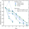Fig. A.1.

SLEDs in velocity-integrated intensities from the simulation compared to observations from Schirm et al. (2014) and Bigiel et al. (2015) of the equivalent regions in the real Antennae. Shown is the average of the three overlap points presented in Bigiel et al. (2010, 2015).

We report a better agreement between our simulated SLEDs and the values of Schirm et al. than between the two observations, which likely originates from differences in beam sizes. While Bigiel et al. focused on the peaks of emission, the pointings in Schirm et al. cover a much larger area, and thus encompass a larger fraction of gas with weaker emission. This is qualitatively closer to the approach followed in our simulations, where our 1 kpc regions gather a wide range of CO-emitting media.

When considering de-normalized values (not shown), our model yields intensities ∼11−18 times higher than that of Schirm et al. (for J_upper ≤ 4, see below), which is compatible with a scale factor of π(4 kpc/2)²/(1 kpc)² ≈ 13 between our surface areas.

We note that our model yields stronger excitations at J_upper ≳ 5, compared to the Schirm et al. data. Following the arguments presented in Sects. 3.6.1 and 4.3, we interpret this difference as a dilution of the contribution from the warm gas (∼1−10 cm⁻³, 10⁴ K) in the larger beams of Schirm.

All Figures

	Fig. 1. Gas density map of the central 12 kpc × 12 kpc of the merger. The connections with the long tidal tails are visible on the left-hand side. The smaller panels show magnifications of the four 1 kpc × 1 kpc regions where our analysis is conducted.
In the text

Fig. 2.

Maps of the depletion time (top left), shear (top right), Mach number (bottom left), and the compressive-to-total ratio of turbulent energy (bottom right). A grayscale map of the gas density is underlaid in the top left panel and is represented as contours in the others to guide the eye. The depletion time and Mach numbers are measured at a scale of 125 pc, using stars younger than 10 Myr for the former, while the shear and compressive-to-total ratio are measured at 50 pc and their maps are density weighted histograms with a bin size of 125 pc. Small circles indicate the positions of minima of depletion times and the dashed squares show our four regions of interest. No clear correlations between these quantities are visible. This is due to the time delay between the onset of a physical trigger and the resulting star formation activity being of the same order of magnitude as the dynamical time of the merger (∼10 Myr).

In the text

	Fig. 3. Normalized mass-weighted gas density PDFs in the four regions and in the entire galaxy (top), and in the two nuclei, with and without the central clouds (i.e., the nuclei themselves; bottom). All regions exhibit a secondary peak of dense gas (≳10⁴ cm⁻³) in contrast with isolated galaxies where these highest densities only correspond to the tails of the distributions.
In the text

Fig. 4.

Top: Schmidt–Kennicutt diagram of the clouds identified in the simulation. The two densest points correspond to the clouds at the galactic centers. The dotted lines mark constant depletion times (from 10 to 110 Myr, in steps of 10 Myr); the dark line corresponds to 40 Myr. Bottom: normalized mass-weighted gas density PDF of these clouds, split into two regimes of depletion times: < 40 and > 60 Myr. Clouds with 40 Myr < t_dep < 60 Myr correspond to the transition regime shown in the top panel and are not considered here for the sake of clarity. The distribution of clouds does not follow a unique power law, but rather a combination of two regimes: clouds with an excess of dense gas have shorter depletion times than those without.

In the text

	Fig. 5. Depletion times as a function of the measurement scale for our four analysis regions, and for a reference isolated progenitor galaxy. While the general trend is common to all regions, details depend on the sub-kpc structure of the ISM and significantly vary from one region to the next, due to different organizations of the clouds set by the kpc-scale environment.
In the text

Fig. 6.

Distribution of depletion times, measured in 30 pc and 500 pc beams on a Cartesian grid (with arbitrary origin, i.e., not centered on peaks of star formation) in the central 6 kpc × 6 kpc of the system. For better statistics, we repeat the measurements by shifting the origin of the grid by several fractions of the beam size, and stack the distributions obtained. Large-scale measurements have a bimodal distribution of short (∼100 Myr) and long (∼2 Gyr) t_dep.

In the text

Fig. 7.

CO spectral line energy distributions for velocity-integrated brightness temperature (left) and velocity-integrated flux density (right), both normalized to CO(1–0), in our four selected regions (filled symbols), in the entire system (global), in the same simulation but during the starburst episode (ULIRG), in a gas-rich clumpy disk (high-redshift), and in a Milky Way-like galaxy (open symbols). The SLEDs of the most actively star-forming regions (nuclei and overlap) resemble that of the Antennae (global and ULIRG), while the arc better matches the high-redshift disk at high J_upper.

In the text

	Fig. 8. Contribution to the CO(J→J-1) line from our four 1 kpc × 1 kpc regions, with respect to the entire system (global, i.e., 10 kpc × 10 kpc). The relative contribution of our four regions varies with J_upper due to differences in the density, temperature, and velocity dispersion of the ISM, particularly in the inter-cloud medium.
In the text

Fig. 9.

The α_CO factor as a function of the surface density of SFR in the four selected regions (1 kpc × 1 kpc, filled symbols), for the entire merger system (global), the same system during the ULIRG phase, a gas-rich clumpy disk (high-redshift) and a Milky Way-like galaxy (open symbols). The error bars show the dispersions of the values, evaluated by varying the line of sight (see Sect. 2.2). Horizontal lines indicate the values commonly used in observations (4.3 for disks, Bolatto et al. 2013, and 0.8 for ULIRGs, Downes & Solomon 1998). Important variations in α_CO are found across the galaxies, due to different interplays of physical processes setting the assembly of star-forming regions, and making our regions lie in between the values traditionally assumed for disks and ULIRGs.

In the text

	Fig. A.1. SLEDs in velocity-integrated intensities from the simulation compared to observations from Schirm et al. (2014) and Bigiel et al. (2015) of the equivalent regions in the real Antennae. Shown is the average of the three overlap points presented in Bigiel et al. (2010, 2015).
In the text

Current usage metrics show cumulative count of Article Views (full-text article views including HTML views, PDF and ePub downloads, according to the available data) and Abstracts Views on Vision4Press platform.

Data correspond to usage on the plateform after 2015. The current usage metrics is available 48-96 hours after online publication and is updated daily on week days.

Initial download of the metrics may take a while.

[1] Agertz, O., Lake, G., Teyssier, R., et al. 2009, MNRAS, 392, 294 [NASA ADS] [CrossRef] [Google Scholar]

[2] Agertz, O., Kravtsov, A. V., Leitner, S. N., & Gnedin, N. Y. 2013, ApJ, 770, 25 [NASA ADS] [CrossRef] [Google Scholar]

[3] Alves, J., Lombardi, M., & Lada, C. J. 2017, A&A, 606, L2 [NASA ADS] [CrossRef] [EDP Sciences] [Google Scholar]

[4] Ashman, K. M., & Zepf, S. E. 2001, AJ, 122, 1888 [NASA ADS] [CrossRef] [Google Scholar]

[5] Ballesteros-Paredes, J., Hartmann, L. W., Vázquez- Semadeni, E., Heitsch, F., & Zamora- Avilés, M. A. 2011, MNRAS, 411, 65 [NASA ADS] [CrossRef] [Google Scholar]

[6] Barnes, J. E. 2004, MNRAS, 350, 798 [NASA ADS] [CrossRef] [Google Scholar]

[7] Barnes, J. E., & Hernquist, L. E. 1991, ApJ, 370, L65 [NASA ADS] [CrossRef] [Google Scholar]

[8] Bastian, N., Trancho, G., Konstantopoulos, I. S., & Miller, B. W. 2009, ApJ, 701, 607 [NASA ADS] [CrossRef] [Google Scholar]

[9] Bate, M. R. 2009, MNRAS, 397, 232 [NASA ADS] [CrossRef] [Google Scholar]

[10] Bate, M. R. 2019, MNRAS, 484, 2341 [NASA ADS] [CrossRef] [Google Scholar]

[11] Bemis, A., & Wilson, C. D. 2019, AJ, 157, 131 [NASA ADS] [CrossRef] [Google Scholar]

[12] Bigiel, F., Leroy, A., Walter, F., et al. 2010, AJ, 140, 1194 [NASA ADS] [CrossRef] [Google Scholar]

[13] Bigiel, F., Leroy, A. K., Blitz, L., et al. 2015, ApJ, 815, 103 [NASA ADS] [CrossRef] [Google Scholar]

[14] Bolatto, A. D., Wolfire, M., & Leroy, A. K. 2013, ARA&A, 51, 207 [Google Scholar]

[15] Bolatto, A. D., Warren, S. R., Leroy, A. K., et al. 2015, ApJ, 809, 175 [NASA ADS] [CrossRef] [Google Scholar]

[16] Bouché, N., Cresci, G., Davies, R., et al. 2007, ApJ, 671, 303 [NASA ADS] [CrossRef] [Google Scholar]

[17] Bournaud, F., Elmegreen, B. G., Teyssier, R., Block, D. L., & Puerari, I. 2010, MNRAS, 409, 1088 [NASA ADS] [CrossRef] [Google Scholar]

[18] Bournaud, F., Chapon, D., Teyssier, R., et al. 2011, ApJ, 730, 4 [NASA ADS] [CrossRef] [Google Scholar]

[19] Bournaud, F., Daddi, E., Weiß, A., et al. 2015, A&A, 575, A56 [NASA ADS] [CrossRef] [EDP Sciences] [Google Scholar]

[20] Brandl, B. R., Snijders, L., den Brok, M., et al. 2009, ApJ, 699, 1982 [NASA ADS] [CrossRef] [Google Scholar]

[21] Cadiou, C., Dubois, Y., & Pichon, C. 2019, A&A, 621, A96 [NASA ADS] [CrossRef] [EDP Sciences] [Google Scholar]

[22] Casasola, V., Bettoni, D., & Galletta, G. 2004, A&A, 422, 941 [NASA ADS] [CrossRef] [EDP Sciences] [Google Scholar]

[23] Chabrier, G., Hennebelle, P., & Charlot, S. 2014, ApJ, 796, 75 [NASA ADS] [CrossRef] [Google Scholar]

[24] Chien, L.-H., & Barnes, J. E. 2010, MNRAS, 407, 43 [NASA ADS] [CrossRef] [MathSciNet] [Google Scholar]

[25] Combes, F., Prugniel, P., Rampazzo, R., & Sulentic, J. W. 1994, A&A, 281, 725 [NASA ADS] [Google Scholar]

[26] Cullen, H., Alexander, P., & Clemens, M. 2006, MNRAS, 366, 49 [Google Scholar]

[27] Daddi, E., Elbaz, D., Walter, F., et al. 2010a, ApJ, 714, L118 [Google Scholar]

[28] Daddi, E., Bournaud, F., Walter, F., et al. 2010b, ApJ, 713, 686 [NASA ADS] [CrossRef] [Google Scholar]

[29] Dale, J. E., Ercolano, B., & Bonnell, I. A. 2012, MNRAS, 424, 377 [NASA ADS] [CrossRef] [Google Scholar]

[30] Downes, D., & Solomon, P. M. 1998, ApJ, 507, 615 [NASA ADS] [CrossRef] [Google Scholar]

[31] Dubois, Y., & Teyssier, R. 2008, A&A, 477, 79 [NASA ADS] [CrossRef] [EDP Sciences] [Google Scholar]

[32] Eisenstein, D. J., & Hut, P. 1998, ApJ, 498, 137 [NASA ADS] [CrossRef] [Google Scholar]

[33] Elmegreen, B. G. 2008, ApJ, 672, 1006 [NASA ADS] [CrossRef] [Google Scholar]

[34] Elmegreen, B. G. 2011, ApJ, 731, 61 [NASA ADS] [CrossRef] [Google Scholar]

[35] Elmegreen, B. G., & Efremov, Y. N. 1997, ApJ, 480, 235 [NASA ADS] [CrossRef] [Google Scholar]

[36] Elmegreen, B. G., & Elmegreen, D. M. 2005, ApJ, 627, 632 [NASA ADS] [CrossRef] [Google Scholar]

[37] Emsellem, E., Renaud, F., Bournaud, F., et al. 2015, MNRAS, 446, 2468 [NASA ADS] [CrossRef] [Google Scholar]

[38] Falceta-Gonçalves, D., Bonnell, I., Kowal, G., Lépine, J. R. D., & Braga, C. A. S. 2015, MNRAS, 446, 973 [NASA ADS] [CrossRef] [Google Scholar]

[39] Federrath, C. 2013, MNRAS, 436, 3167 [NASA ADS] [CrossRef] [Google Scholar]

[40] Federrath, C., & Klessen, R. S. 2012, ApJ, 761, 156 [NASA ADS] [CrossRef] [Google Scholar]

[41] Federrath, C., Roman-Duval, J., Klessen, R. S., Schmidt, W., & Mac Low, M.-M. 2010, A&A, 512, A81 [NASA ADS] [CrossRef] [EDP Sciences] [Google Scholar]

[42] Feldmann, R., Gnedin, N. Y., & Kravtsov, A. V. 2012, ApJ, 758, 127 [NASA ADS] [CrossRef] [Google Scholar]

[43] Fensch, J., Renaud, F., Bournaud, F., et al. 2017, MNRAS, 465, 1934 [NASA ADS] [CrossRef] [Google Scholar]

[44] Fukui, Y., Ohama, A., Hanaoka, N., et al. 2014, ApJ, 780, 36 [NASA ADS] [CrossRef] [Google Scholar]

[45] Genel, S., Vogelsberger, M., Nelson, D., et al. 2013, MNRAS, 435, 1426 [NASA ADS] [CrossRef] [Google Scholar]

[46] Genzel, R., Tacconi, L. J., Gracia-Carpio, J., et al. 2010, MNRAS, 407, 2091 [NASA ADS] [CrossRef] [Google Scholar]

[47] Goodwin, S. P., Nutter, D., Kroupa, P., Ward-Thompson, D., & Whitworth, A. P. 2008, A&A, 477, 823 [NASA ADS] [CrossRef] [EDP Sciences] [Google Scholar]

[48] Graciá-Carpio, J., García-Burillo, S., Planesas, P., Fuente, A., & Usero, A. 2008, A&A, 479, 703 [NASA ADS] [CrossRef] [EDP Sciences] [Google Scholar]

[49] Greve, T. R., Bertoldi, F., Smail, I., et al. 2005, MNRAS, 359, 1165 [NASA ADS] [CrossRef] [Google Scholar]

[50] Grisdale, K., Agertz, O., Romeo, A. B., Renaud, F., & Read, J. I. 2017, MNRAS, 466, 1093 [NASA ADS] [CrossRef] [Google Scholar]

[51] Grisdale, K., Agertz, O., Renaud, F., et al. 2019, MNRAS, submitted [arXiv:1902.00518] [Google Scholar]

[52] Haas, M., Chini, R., & Klaas, U. 2005, A&A, 433, L17 [NASA ADS] [CrossRef] [EDP Sciences] [Google Scholar]

[53] Hancock, M., Smith, B. J., Struck, C., Giroux, M. L., & Hurlock, S. 2009, AJ, 137, 4643 [NASA ADS] [CrossRef] [Google Scholar]

[54] Hennebelle, P., & Chabrier, G. 2011, ApJ, 743, L29 [NASA ADS] [CrossRef] [Google Scholar]

[55] Hennebelle, P., & Falgarone, E. 2012, A&ARv, 20, 55 [NASA ADS] [CrossRef] [Google Scholar]

[56] Hernquist, L., & Katz, N. 1989, ApJS, 70, 419 [NASA ADS] [CrossRef] [Google Scholar]

[57] Herrera, C. N., Boulanger, F., Nesvadba, N. P. H., & Falgarone, E. 2012, A&A, 538, L9 [NASA ADS] [CrossRef] [EDP Sciences] [Google Scholar]

[58] Hopkins, P. F., Narayanan, D., Murray, N., & Quataert, E. 2013a, MNRAS, 433, 69 [NASA ADS] [CrossRef] [Google Scholar]

[59] Hopkins, P. F., Cox, T. J., Hernquist, L., et al. 2013b, MNRAS, 430, 1901 [NASA ADS] [CrossRef] [Google Scholar]

[60] Hopkins, P. F., Wetzel, A., Kereš, D., et al. 2018, MNRAS, 480, 800 [NASA ADS] [CrossRef] [Google Scholar]

[61] Inoue, T., & Fukui, Y. 2013, ApJ, 774, L31 [NASA ADS] [CrossRef] [Google Scholar]

[62] Jog, C. J., & Solomon, P. M. 1992, ApJ, 387, 152 [NASA ADS] [CrossRef] [Google Scholar]

[63] Johnson, K. E., Leroy, A. K., Indebetouw, R., et al. 2015, ApJ, 806, 35 [NASA ADS] [CrossRef] [Google Scholar]

[64] Kaneko, H., Kuno, N., Iono, D., et al. 2017, PASJ, 69, 66 [NASA ADS] [CrossRef] [Google Scholar]

[65] Karl, S. J., Naab, T., Johansson, P. H., et al. 2010, ApJ, 715, L88 [NASA ADS] [CrossRef] [Google Scholar]

[66] Keel, W. C., Kennicutt, Jr., R. C., Hummel, E., & van der Hulst, J. M. 1985, AJ, 90, 708 [NASA ADS] [CrossRef] [Google Scholar]

[67] Kennicutt, Jr., R. C. 1998, ARA&A, 36, 189 [Google Scholar]

[68] Kennicutt, R. C., & Evans, N. J. 2012, ARA&A, 50, 531 [NASA ADS] [CrossRef] [Google Scholar]

[69] Klaas, U., Nielbock, M., Haas, M., Krause, O., & Schreiber, J. 2010, A&A, 518, L44 [NASA ADS] [CrossRef] [EDP Sciences] [Google Scholar]

[70] Knapen, J. H., Cisternas, M., & Querejeta, M. 2015, MNRAS, 454, 1742 [NASA ADS] [CrossRef] [Google Scholar]

[71] Körtgen, B., Federrath, C., & Banerjee, R. 2019, MNRAS, 482, 5233 [NASA ADS] [CrossRef] [Google Scholar]

[72] Kraljic, K. 2014, Links Between Galaxy Evolution, Morphology and Internal Physical Processes (PhD Thesis, Universite Paris 11, 2014) [Google Scholar]

[73] Kravtsov, A. V. 2003, ApJ, 590, L1 [NASA ADS] [CrossRef] [Google Scholar]

[74] Krips, M., Martín, S., Eckart, A., et al. 2011, ApJ, 736, 37 [NASA ADS] [CrossRef] [Google Scholar]

[75] Kritsuk, A. G., Norman, M. L., Padoan, P., & Wagner, R. 2007, ApJ, 665, 416 [NASA ADS] [CrossRef] [Google Scholar]

[76] Krumholz, M. R., & Dekel, A. 2010, MNRAS, 406, 112 [NASA ADS] [CrossRef] [Google Scholar]

[77] Krumholz, M. R., & Gnedin, N. Y. 2011, ApJ, 729, 36 [NASA ADS] [CrossRef] [Google Scholar]

[78] Krumholz, M. R., & Matzner, C. D. 2009, ApJ, 703, 1352 [NASA ADS] [CrossRef] [Google Scholar]

[79] Krumholz, M. R., Dekel, A., & McKee, C. F. 2012, ApJ, 745, 69 [NASA ADS] [CrossRef] [Google Scholar]

[80] Leroy, A. K., Walter, F., Sandstrom, K., et al. 2013, AJ, 146, 19 [NASA ADS] [CrossRef] [Google Scholar]

[81] Leroy, A. K., Schinnerer, E., Hughes, A., et al. 2017, ApJ, 846, 71 [NASA ADS] [CrossRef] [Google Scholar]

[82] Liszt, H. S., & Pety, J. 2012, A&A, 541, A58 [NASA ADS] [CrossRef] [EDP Sciences] [Google Scholar]

[83] Liszt, H. S., Pety, J., & Lucas, R. 2010, A&A, 518, A45 [NASA ADS] [CrossRef] [EDP Sciences] [Google Scholar]

[84] Magnelli, B., Lutz, D., Santini, P., et al. 2012, A&A, 539, A155 [NASA ADS] [CrossRef] [EDP Sciences] [Google Scholar]

[85] Maji, M., Zhu, Q., Li, Y., et al. 2017, ApJ, 844, 108 [NASA ADS] [CrossRef] [Google Scholar]

[86] Martinez-Badenes, V., Lisenfeld, U., Espada, D., et al. 2012, A&A, 540, A96 [NASA ADS] [CrossRef] [EDP Sciences] [Google Scholar]

[87] Matzner, C. D. 2002, ApJ, 566, 302 [NASA ADS] [CrossRef] [Google Scholar]

[88] Meidt, S. E., Schinnerer, E., García-Burillo, S., et al. 2013, ApJ, 779, 45 [NASA ADS] [CrossRef] [Google Scholar]

[89] Michiyama, T., Iono, D., Nakanishi, K., et al. 2016, PASJ, 68, 96 [NASA ADS] [CrossRef] [Google Scholar]

[90] Moreno, J., Bluck, A. F. L., Ellison, S. L., et al. 2013, MNRAS, 436, 1765 [NASA ADS] [CrossRef] [Google Scholar]

[91] Motte, F., Nguyên Luong, Q., Schneider, N., et al. 2014, A&A, 571, A32 [NASA ADS] [CrossRef] [EDP Sciences] [Google Scholar]

[92] Motte, F., Nony, T., Louvet, F., et al. 2018, Nat. Astron., 2, 478 [NASA ADS] [CrossRef] [Google Scholar]

[93] Myers, A. T., Krumholz, M. R., Klein, R. I., & McKee, C. F. 2011, ApJ, 735, 49 [NASA ADS] [CrossRef] [Google Scholar]

[94] Narayanan, D., Krumholz, M., Ostriker, E. C., & Hernquist, L. 2011, MNRAS, 418, 664 [NASA ADS] [CrossRef] [Google Scholar]

[95] Nehlig, F., Vollmer, B., & Braine, J. 2016, A&A, 587, A108 [NASA ADS] [CrossRef] [EDP Sciences] [Google Scholar]

[96] Ohlin, L., Renaud, F., & Agertz, O. 2019, MNRAS, 485, 3887 [NASA ADS] [CrossRef] [Google Scholar]

[97] Padoan, P., & Nordlund, Å. 2011, ApJ, 730, 40 [NASA ADS] [CrossRef] [Google Scholar]

[98] Pan, H.-A., Lin, L., Hsieh, B.-C., et al. 2018, ApJ, 868, 132 [NASA ADS] [CrossRef] [Google Scholar]

[99] Papadopoulos, P. P., van der Werf, P. P., Xilouris, E. M., et al. 2012, MNRAS, 426, 2601 [NASA ADS] [CrossRef] [Google Scholar]

[100] Pereira-Santaella, M., Colina, L., García-Burillo, S., et al. 2016, A&A, 587, A44 [NASA ADS] [CrossRef] [EDP Sciences] [Google Scholar]

[101] Renaud, F., Kraljic, K., & Bournaud, F. 2012, ApJ, 760, L16 [NASA ADS] [CrossRef] [Google Scholar]

[102] Renaud, F., Bournaud, F., Emsellem, E., et al. 2013, MNRAS, 436, 1836 [NASA ADS] [CrossRef] [Google Scholar]

[103] Renaud, F., Bournaud, F., Kraljic, K., & Duc, P.-A. 2014, MNRAS, 442, L33 [NASA ADS] [CrossRef] [Google Scholar]

[104] Renaud, F., Bournaud, F., & Duc, P.-A. 2015a, MNRAS, 446, 2038 [NASA ADS] [CrossRef] [Google Scholar]

[105] Renaud, F., Bournaud, F., Emsellem, E., et al. 2015b, MNRAS, 454, 3299 [NASA ADS] [CrossRef] [Google Scholar]

[106] Renaud, F., Athanassoula, E., Amram, P., et al. 2018, MNRAS, 473, 585 [NASA ADS] [CrossRef] [Google Scholar]

[107] Renaud, F., Bournaud, F., Daddi, E., & Weiß, A. 2019, A&A, 621, A104 [NASA ADS] [CrossRef] [EDP Sciences] [Google Scholar]

[108] Rogers, H., & Pittard, J. M. 2013, MNRAS, 431, 1337 [NASA ADS] [CrossRef] [Google Scholar]

[109] Rosen, A., & Bregman, J. N. 1995, ApJ, 440, 634 [NASA ADS] [CrossRef] [Google Scholar]

[110] Saintonge, A., Kauffmann, G., Wang, J., et al. 2011, MNRAS, 415, 61 [NASA ADS] [CrossRef] [Google Scholar]

[111] Saito, T., Iono, D., Xu, C. K., et al. 2016, PASJ, 68, 20 [NASA ADS] [CrossRef] [Google Scholar]

[112] Salim, D. M., Federrath, C., & Kewley, L. J. 2015, ApJ, 806, L36 [NASA ADS] [CrossRef] [Google Scholar]

[113] Sanders, D. B., & Mirabel, I. F. 1996, ARA&A, 34, 749 [NASA ADS] [CrossRef] [Google Scholar]

[114] Sandstrom, K. M., Leroy, A. K., Walter, F., et al. 2013, ApJ, 777, 5 [NASA ADS] [CrossRef] [Google Scholar]

[115] Schirm, M. R. P., Wilson, C. D., Parkin, T. J., et al. 2014, ApJ, 781, 101 [NASA ADS] [CrossRef] [Google Scholar]

[116] Schruba, A., Leroy, A. K., Walter, F., Sandstrom, K., & Rosolowsky, E. 2010, ApJ, 722, 1699 [NASA ADS] [CrossRef] [Google Scholar]

[117] Schweizer, F., Burns, C. R., Madore, B. F., et al. 2008, AJ, 136, 1482 [NASA ADS] [CrossRef] [Google Scholar]

[118] Scudder, J. M., Ellison, S. L., Torrey, P., Patton, D. R., & Mendel, J. T. 2012, MNRAS, 426, 549 [NASA ADS] [CrossRef] [Google Scholar]

[119] Semenov, V. A., Kravtsov, A. V., & Gnedin, N. Y. 2017, ApJ, 845, 133 [NASA ADS] [CrossRef] [Google Scholar]

[120] Semenov, V. A., Kravtsov, A. V., & Gnedin, N. Y. 2018, ApJ, 861, 4 [NASA ADS] [CrossRef] [Google Scholar]

[121] Smith, B. J., Struck, C., Hancock, M., et al. 2008, AJ, 135, 2406 [NASA ADS] [CrossRef] [Google Scholar]

[122] Solomon, P. M., & Sage, L. J. 1988, ApJ, 334, 613 [NASA ADS] [CrossRef] [Google Scholar]

[123] Strong, A. W., Moskalenko, I. V., Reimer, O., Digel, S., & Diehl, R. 2004, A&A, 422, L47 [NASA ADS] [CrossRef] [EDP Sciences] [Google Scholar]

[124] Sun, J., Leroy, A. K., Schruba, A., et al. 2018, ApJ, 860, 172 [NASA ADS] [CrossRef] [Google Scholar]

[125] Sutherland, R. S., & Dopita, M. A. 1993, ApJS, 88, 253 [NASA ADS] [CrossRef] [Google Scholar]

[126] Tacconi, L. J., Genzel, R., Smail, I., et al. 2008, ApJ, 680, 246 [NASA ADS] [CrossRef] [PubMed] [Google Scholar]

[127] Tacconi, L. J., Genzel, R., Neri, R., et al. 2010, Nature, 463, 781 [Google Scholar]

[128] Takahira, K., Tasker, E. J., & Habe, A. 2014, ApJ, 792, 63 [NASA ADS] [CrossRef] [Google Scholar]

[129] Tan, J. C. 2000, ApJ, 536, 173 [NASA ADS] [CrossRef] [Google Scholar]

[130] Tasker, E. J., & Tan, J. C. 2009, ApJ, 700, 358 [NASA ADS] [CrossRef] [Google Scholar]

[131] Teyssier, R. 2002, A&A, 385, 337 [NASA ADS] [CrossRef] [EDP Sciences] [Google Scholar]

[132] Teyssier, R., Chapon, D., & Bournaud, F. 2010, ApJ, 720, L149 [NASA ADS] [CrossRef] [Google Scholar]

[133] Teyssier, R., Pontzen, A., Dubois, Y., & Read, J. I. 2013, MNRAS, 429, 3068 [NASA ADS] [CrossRef] [Google Scholar]

[134] Tomičić, N., Hughes, A., Kreckel, K., et al. 2018, ApJ, 869, L38 [NASA ADS] [CrossRef] [Google Scholar]

[135] Ueda, J., Iono, D., Petitpas, G., et al. 2012, ApJ, 745, 65 [NASA ADS] [CrossRef] [Google Scholar]

[136] Usero, A., Leroy, A. K., Walter, F., et al. 2015, AJ, 150, 115 [NASA ADS] [CrossRef] [Google Scholar]

[137] Vazquez-Semadeni, E. 1994, ApJ, 423, 681 [NASA ADS] [CrossRef] [Google Scholar]

[138] Vázquez-Semadeni, E., Gómez, G. C., Jappsen, A.-K., Ballesteros-Paredes, J., & Klessen, R. S. 2009, ApJ, 707, 1023 [NASA ADS] [CrossRef] [Google Scholar]

[139] Violino, G., Ellison, S. L., Sargent, M., et al. 2018, MNRAS, 476, 2591 [NASA ADS] [CrossRef] [Google Scholar]

[140] Wang, Z., Fazio, G. G., Ashby, M. L. N., et al. 2004, ApJS, 154, 193 [NASA ADS] [CrossRef] [Google Scholar]

[141] Weilbacher, P. M., Monreal-Ibero, A., Verhamme, A., et al. 2018, A&A, 611, A95 [NASA ADS] [CrossRef] [EDP Sciences] [Google Scholar]

[142] Weiß, A., Walter, F., & Scoville, N. Z. 2005, A&A, 438, 533 [NASA ADS] [CrossRef] [EDP Sciences] [Google Scholar]

[143] Whitmore, B. C., Zhang, Q., Leitherer, C., et al. 1999, AJ, 118, 1551 [NASA ADS] [CrossRef] [Google Scholar]

[144] Whitmore, B. C., Brogan, C., Chandar, R., et al. 2014, ApJ, 795, 156 [NASA ADS] [CrossRef] [Google Scholar]

[145] Wilson, C. D., Scoville, N., Madden, S. C., & Charmandaris, V. 2003, ApJ, 599, 1049 [NASA ADS] [CrossRef] [Google Scholar]

[146] Yao, L., Seaquist, E. R., Kuno, N., & Dunne, L. 2003, ApJ, 588, 771 [NASA ADS] [CrossRef] [Google Scholar]

[147] Zhang, Q., Fall, S. M., & Whitmore, B. C. 2001, ApJ, 561, 727 [NASA ADS] [CrossRef] [Google Scholar]

[148] Zhu, M., Seaquist, E. R., & Kuno, N. 2003, ApJ, 588, 243 [NASA ADS] [CrossRef] [Google Scholar]

A diversity of starburst-triggering mechanisms in interacting galaxies and their signatures in CO emission

1. Introduction

2. Method

2.1. Numerical method

2.2. CO emission

2.3. Regions of interest

3. Results

3.1. The triggers of star formation and their delays

3.2. Excess of dense gas in the star-forming regions

3.3. Variations in depletion time

3.4. Scale dependence

3.5. Long depletion times in the nuclei

3.6. CO emission

3.6.1. Spectral line energy distributions

3.6.2. Spatial variations of αCO

4. Discussion

4.1. Compressive turbulence and the shape of the density PDF

4.2. The galactic nuclei as collision environments

4.3. Imprint of the ISM structure on the CO emission

4.4. The importance of capturing the structure of the cold ISM

5. Conclusions

Acknowledgments

References

Appendix A: Comparison of CO SLEDs with observations

All Figures

3.6.2. Spatial variations of α_CO