| Issue |
A&A
Volume 625, May 2019
|
|
|---|---|---|
| Article Number | A132 | |
| Number of page(s) | 15 | |
| Section | Stellar structure and evolution | |
| DOI | https://doi.org/10.1051/0004-6361/201935046 | |
| Published online | 27 May 2019 | |
Constraining mixing in massive stars in the Small Magellanic Cloud⋆
Argelander-Institut für Astronomie, Universität Bonn, Auf dem Hügel 71, 53121 Bonn, Germany
e-mail: aschoot@astro.uni-bonn.de
Received:
11
January
2019
Accepted:
25
March
2019
Context. The evolution of massive stars is strongly influenced by internal mixing processes such as semiconvection, convective core overshooting, and rotationally induced mixing. None of these processes are currently well constrained.
Aims. We investigate models for massive stars in the Small Magellanic Cloud (SMC), for which stellar-wind mass loss is less important than for their metal-rich counterparts. We aim to constrain the various mixing efficiencies by comparing model results to observations.
Methods. For this purpose, we use the stellar-evolution code MESA to compute more than 60 grids of detailed evolutionary models for stars with initial masses of 9…100 M⊙, assuming different combinations of mixing efficiencies of the various processes in each grid. Our models evolve through core hydrogen and helium burning, such that they can be compared with the massive main sequence and supergiant population of the SMC.
Results. We find that for most of the combinations of the mixing efficiencies, models in a wide mass range spend core-helium burning either only as blue supergiants, or only as red supergiants. The latter case corresponds to models that maintain a shallow slope of the hydrogen/helium (H/He) gradient separating the core and the envelope of the models. Only a small part of the mixing parameter space leads to models that produce a significant number of blue and red supergiants, which are both in abundance in the SMC. Some of our grids also predict a cut-off in the number of red supergiants above log L/L⊙ = 5…5.5. Interestingly, these models contain steep H/He gradients, as is required to understand the hot, hydrogen-rich Wolf-Rayet stars in the SMC. We find that unless it is very fast, rotation has a limited effect on the H/He profiles in our models.
Conclusions. While we use specific implementations of the considered mixing processes, they comprehensively probe the two first-order structural parameters, the core mass and the H/He gradient in the core-envelope interface. Our results imply that in massive stars, mixing during the main-sequence evolution leads to a moderate increase in the helium core masses, and also that the H/He gradients above the helium cores become very steep. Our model grids can be used to further refine the various mixing efficiencies with the help of future observational surveys of the massive stars in the SMC, and thereby help to considerably reduce the uncertainties in models of massive star evolution.
Key words: stars: massive / stars: early-type / stars: Wolf-Rayet / stars: interiors / stars: rotation / stars: evolution
Tables of evolutionary tracks are only available at the CDS via anonymous ftp to cdsarc.u-strasbg.fr (130.79.128.5) or via http://cdsarc.u-strasbg.fr/viz-bin/qcat?J/A+A/625/A132
© ESO 2019
1. Introduction
Massive stars play a central role in astrophysics. They dominate the evolution of star forming galaxies by providing chemical enrichment, ionizing radiation, and mechanical feedback (e.g., Hopkins et al. 2014). Massive stars also produce a variety of transient phenomena, like supernovae (SNe), long-duration gamma-ray bursts (lGRBs), and merging black holes emitting gravitational waves. These events can be so bright that they are observable up to high redshift, allowing us to study the early universe. In fact, lGRBs (Graham & Fruchter 2017), superluminous SNe (Chen et al. 2017; Schulze et al. 2018), and likely also massive black hole mergers (Belczynski et al. 2010) appear predominantly in low-metallicity galaxies. The implication is that massive-star evolution can proceed differently in the early universe compared to that in the Milky Way. However, at high redshift, massive stars cannot be observed individually until they explode.
It is therefore important to study the existing low-metallicity massive stars that are nearby, which are concentrated in star forming dwarf galaxies. A unique environment for this is provided by the Small Magellanic Cloud (SMC), which at a distance of ∼60 kpc allows the detailed study of individual stars. With a metal content of about one fifth of the solar value (Venn 1999; Korn et al. 2000), it is representative of massive star forming galaxies at a redshift around z = 3 (Kewley & Kobulnicky 2007).
Evolutionary models of massive stars are hampered by our ignorance of two physical ingredients, mass loss and internal mixing. Also in this respect, it is beneficial to focus on the low-metallicity environment of the SMC, where stellar winds appear to be significantly weaker than in the Milky Way (Mokiem et al. 2007). For example, current evolutionary models predict that stars above ∼25 M⊙ in the Galaxy lose more than 10% of their initial mass through stellar winds during the main-sequence evolution, while in the SMC this happens only for stars above ∼60 M⊙ (Brott et al. 2011). By considering massive stars in the SMC, we aim to exploit this feature, which allows us, at least below a certain threshold mass, to focus on internal mixing as the major uncertainty in massive single star evolution.
The evolution of massive stars is known to sensitively depend on a number of internal-mixing processes (Langer 2012). The most important one is certainly convection, and “convective overshooting”, that is, mixing at the boundaries of convective regions (Maeder & Meynet 1988; Alongi et al. 1993), which affects the core masses and lifetimes of all phases of massive star evolution. Semiconvection is a further important but not well-understood process that determines the timescale of mixing in layers with a stabilizing gradient in the mean molecular weight (Langer et al. 1983). It regulates the hydrogen/helium (H/He) gradient at the core-envelope interface in massive stars, thereby sensitively influencing their post-main-sequence radius evolution (Langer 1991; Stothers & Chin 1992; Langer & Maeder 1995). It should be noted that a deep understanding of what drives a stellar model to a blue or red solution after core hydrogen burning is still absent. Various ideas have been proposed and discussed (e.g., Höppner & Weigert 1973; Renzini et al. 1992; Iben 1993; Sugimoto & Fujimoto 2000; Stancliffe et al. 2009) but a consensus remains to be reached. Finally, rotationally induced mixing may affect the evolution of massive stars, at least for the fraction of them that rotate rapidly (Maeder & Meynet 2000; Heger et al. 2000; Yoon et al. 2006). These mixing processes will not only affect the evolution of the surface properties of massive stars, but also determine their internal structure, and are therefore important, for example, for realistic pre-SN models.
While the individual effects of the efficiency of these mixing processes on evolutionary models are well known, and in many cases have been for decades, it is highly uncertain which efficiencies are realistic At present, this is difficult to gauge from first-principle multi-dimensional calculations (Merryfield 1995; Grossman & Taam 1996; Canuto 1999; Zaussinger & Spruit 2013). At the same time, even when the influence of mass loss on the evolution can be neglected, it is also difficult to constrain the mixing efficiencies observationally, as all three processes may act at the same time.
Here, we take advantage of the increase in computing power of recent decades, which allows us to explore the whole realistic parameter space for more than one mixing process simultaneously. We compute 66 grids of massive star evolutionary models with 11 initial masses per grid, giving a total of 726 evolutionary sequences, where we vary the assumptions on the efficiency of overshooting, semiconvection, and, by choosing different initial rotational velocities, of rotationally induced mixing. We then explore which combinations of mixing efficiencies lead to models that are consistent with the available observational constraints.
A second recent applicable development is the study by Schootemeijer & Langer (2018). These authors investigated Wolf-Rayet (WR) stars in the SMC and found that the progenitor stars of apparently single WR stars contain a H/He gradient that is about ten times steeper than the one emerging during core hydrogen burning as a result of the retreating convective core. They suggested that this steep gradient could be caused by internal mixing. We therefore explore in which part of the mixing parameter space we can reproduce this gradient.
In Sect. 2, we explain the method that we used to obtain our results, which are presented in Sect. 3. In Sect. 4 we compare our results with earlier work. We interpret the further implications of observed blue and red supergiant populations on the efficiency of overshooting and semiconvection in Sect. 5. In Sect. 6 we discuss the robustness of our results and finally we present the conclusions of our work in Sect. 7.
2. Method
We used MESA1 (Paxton et al. 2011, 2013, 2015, 2018, version 10108) to simulate our grid of stellar-evolution models. MESA is a one-dimensional stellar-evolution code that solves the stellar structure equations. For the physics assumptions we followed Schootemeijer & Langer (2018), who in turn adopted among other things the SMC chemical composition and a wind mass loss recipe as in Brott et al. (2011). Below, we highlight the most important physics assumptions.
The choice of wind-mass-loss recipe depends on the temperature Teff and surface hydrogen mass fraction Xs. For hot stars (Teff > 25 kK) that are hydrogen rich (Xs > 0.7) we adopted the prescription of Vink et al. (2001). For hot hydrogen-poor stars (Xs < 0.4) we used the wind of Hamann et al. (1995) divided by ten. We linearly interpolated between the predicted log Ṁ given by both prescriptions in cases where 0.4 < Xs < 0.7. For cold stars (Teff ≲ 25 kK) we used the prescription from Nieuwenhuijzen & de Jager (1990) in cases where it predicts a mass-loss rate higher than that of Vink et al. (2001). Due to its high opacity, iron is the main driver of stellar winds. We scaled all winds to the iron abundance rather than the metallicity Z. The stellar winds thus scale as Ṁ ∝ (XFe/XFe, ⊙)0.85, where the factor 0.85 is the metallicity dependence found by Vink et al. (2001). Here, XFe, ⊙ = 0.00124 (Grevesse et al. 1996).
The initial composition of our models is based on various observations. The iron mass fraction XFe, SMC follows from Venn (1999), who found that [Fe/H]SMC = −0.4. The mass fractions from the elements C, N, O, and Mg are those as listed in Brott et al. (2011). The helium mass fraction (Y) is 0.252. Finally, the hydrogen mass fraction is calculated as X = 1 − Y − Z.
We adopted the Ledoux criterion for convection. In regions where convective mixing occurs, we employed the standard mixing length theory (Böhm-Vitense 1958) with a mixing length parameter of αMLT = 1.5. In superadiabatic regions that possess a stabilizing mean molecular weight (μ) gradient, we assumed semiconvective mixing to occur. The efficiency of semiconvective mixing in our models is controlled by the scaling factor αsc (Langer et al. 1983). We explored the range αsc = 0.01, …, 300. The mixing region above hydrogen-burning convective cores is extended by a distance of αovHP, where HP is the pressure scale height at the convective core boundary (i.e., we use step overshooting). In our models, we considered the range αov = 0.0, …, 0.55. The range of initial masses that we explored is M = 9, …, 100 M⊙.
We investigated which spatial and temporal resolution gives the most convergent results. We found that high spatial resolution (mesh_delta_coeff = 0.3 in MESA lingo – this is a factor used to obtain the maximum difference in the log of the pressure, temperature, and helium mass fraction between two adjacent cells; it is multiplied by the default values of Paxton et al. 2011) and moderate time resolution (varcontrol_target = 7d-4) accomplishes this, that is, our results appear unaffected by the resolution in the non-rotating case. It is known that different numerical choices, for example, time resolution, affect the exact amount of rotational mixing that takes place (Lau et al. 2014). Therefore, we chose the MESA standard value for time resolution for our models including rotation (varcontrol_target = 1d-4.)
As an example of how we measure the slope of the H/He-gradient, we show a model from our grid in Fig. 1 that has just exhausted hydrogen in its core. The retreat of the convective core during the main-sequence evolution has left a nearly linear H/He gradient, which is well represented by a constant slope of dX/dQ = 1.5 (red line in Fig. 1). Here, Q is a relative mass coordinate, with Q = 1 corresponding to the point where the linearly approximated hydrogen-profile reaches the initial hydrogen mass fraction of the star: X = Xini (see Schootemeijer & Langer 2018).
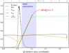 |
Fig. 1. Various quantities of our 16 M⊙ stellar model computed with αov = 0.11 after core hydrogen depletion as a function of the internal mass coordinate. The model is undergoing hydrogen shell burning, as indicated by the relative rate of nuclear energy production (black dotted line). The hydrogen mass fraction is shown in green. The part of the hydrogen profile that was used to fit the H/He gradient dX/dQ (see main text) is shown with a dashed line; the rest is shown with a dot-dashed line. The resulting fit is shown as a straight red line. The semiconvective region, where the radiative temperature gradient ∇rad exceeds the adiabatic temperature gradient ∇ad in the presence of a stabilizing mean molecular weight gradient, is shaded in blue. |
Our evolutionary sequences are discontinued upon core helium exhaustion (Yc = 0.01). Stars in later, short-lived burning phases are not expected to constitute a significant fraction of massive star populations. While we do not compute binary models, we discuss the potential impact of this omission in Sect. 6.
3. Results
Below, we investigate in Sect. 3.1 the main effects that overshooting and semiconvection have on the evolution of massive star models in the Hertzsprung–Russell diagram (HRD). Subsequently, we discuss in more detail how overshooting, semiconvection, and rotational mixing affect the internal chemical profiles of our models in Sect. 3.2.
3.1. Effects of mixing on the evolution in the Hertzsprung–Russell diagram
3.1.1. Main sequence evolution
The main mixing processes that play a role during the main sequence (MS) evolution are convection, overshooting, and rotational mixing. Semiconvection becomes important only after the MS stage (we elaborate on this in Sect. 3.2). As is well known (e.g., Cloutman & Whitaker 1980), mixing of layers above the convective core increases the MS lifetime and allows stars to end core hydrogen burning at lower surface temperatures and higher luminosities. In most evolutionary models in the literature, such mixing is assumed to be due to core overshooting, but rotational mixing can have a similar effect (see e.g., Heger et al. 2000). The effects of overshooting described above do emerge in Fig. 2, where the MS broadens as αov is increased (i.e., from the top to bottom panels). In the same figure, it can be seen that the MS evolution is unaffected by the efficiency of semiconvection.
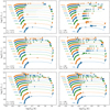 |
Fig. 2. Evolutionary tracks in the HRD for models computed with different efficiencies of overshooting and semiconvective mixing, from core hydrogen ignition to core helium exhaustion. Left panel: models computed with inefficient semiconvective mixing (αsc = 0.01) for three different overshooting parameters (αov = 0.11, 0.33, and 0.55), while the right panels: models computed with efficient semiconvection (αsc = 100), for the same three different values of the overshooting parameter. The time difference between two neighboring markers on a track is 50 000 yr. A circular marker means that the model is core hydrogen burning, a diamond indicates core helium burning. The models shown are nonrotating. |
We further demonstrate the effects of overshooting and rotational mixing on the MS evolution in Fig. 3, where we display the terminal-age main sequence (TAMS) for evolutionary sequences with different initial rotation velocities (0, 225 and 375 km s−1). We see that rotation mostly leads to slightly lower TAMS temperatures, like overshooting. There are two reasons for this. First, the central mixing region can be extended, although this effect is typically small in our models (cf. Sect. 3.2.4). Second, because of rotation, the temperatures decrease as a result of the centrifugal acceleration reducing the effective gravity (see e.g., Chieffi & Limongi 2013; Köhler et al. 2015, their Fig. 3). In our model sequences, this effect is stronger at the TAMS than at the zero-age main sequence (ZAMS), because during the MS evolution the ratio of rotational to critical rotational velocity increases. This effect is reduced for the highest considered masses, where stellar winds induce a spin-down of the models. At the higher masses, rotational mixing is predicted to be the most efficient. If strong enough, the effects of rotation can push stars to the hot side of the HRD (e.g., Maeder 1987; Yoon & Langer 2005; Chieffi & Limongi 2013). As a result, the TAMS in Fig. 3 bends to higher temperatures for the most massive stars with a higher initial rotation velocity.
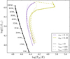 |
Fig. 3. Hertzsprung–Russell diagram showing the terminal-age main sequence (TAMS) lines emerging from model grids computed with different combinations of overshooting αov and initial rotation velocity vrot, i (in units of km s−1). The semiconvective mixing efficiency is fixed to αsc = 1, but the TAMS-lines are insensitive to this parameter. The black lines indicate the corresponding zero age main sequences. |
3.1.2. Post-main-sequence evolution
In many of our model populations, the ratio of blue to red supergiant lifetime during core helium burning depends strongly on the efficiency of semiconvective mixing during the early stages of hydrogen shell burning (as discussed by, e.g., Langer 1991; Stothers & Chin 1992; Langer & Maeder 1995). If such mixing is inefficient, the model sequences tend to favor red supergiant (RSG) solutions. This is illustrated in Fig. 2, where the left panels show that all model sequences with αsc = 0.01 (i.e., very inefficient semiconvection) spend virtually their entire helium-core-burning lifetime in a narrow effective temperature range as RSGs. In cases where semiconvection is very efficient (αsc = 100, right panels in Fig. 2), the lifetime in the blue supergiant (BSG) regime is enhanced. In particular when efficient semiconvection is combined with low overshooting, our evolutionary sequences spend most of the core helium burning as BSGs. For large values of αov, the difference between low and high αsc vanishes, because in that case semiconvective regions rarely develop in the deep hydrogen envelope. We discuss this in more detail in Sect. 3.2.2. Appendix A provides a figure similar to Fig. 2 that shows more combinations of αsc and αov (Fig. A.1).
To further quantify how our evolutionary models evolve during core helium burning, we compute tRSG/tHe burn, which is the fraction of time spent as an RSG. Following Drout et al. (2009), we adopt a temperature threshold for RSGs of Teff < 4800 K. The result is shown in Fig. 4. We find that if semiconvection is inefficient (αsc ≤ 0.3) or overshooting is high (αov ≥ 0.44), our models tend to be RSGs during core helium burning. The only exception to this occurs at the highest masses: in that case, the more massive a star is and the larger the overshooting, the less time it spends as an RSG. The reason for this is that the stellar winds in these models (which become stronger with mass) are able to remove a significant fraction of the hydrogen envelope (which becomes less massive with higher overshooting). If the mass of the hydrogen envelope becomes small enough, the models predict temperatures high enough for them to appear yellow or blue.
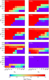 |
Fig. 4. The fractional core helium burning lifetime that our model sequences spend as a red supergiant (color coded), as function of the adopted values of αsc and αov in our model grids, for ten different considered initial masses. Each pixel represents one stellar-evolution sequence. The cross indicates the parameters chosen in the models of (Brott et al. 2011). |
Models in the bottom right of the plots in Fig. 4, i.e., with low overshooting (αov ≤ 0.22) and efficient semiconvection, often fail to reach RSG temperatures during core helium burning. Models with efficient semiconvection and intermediate overshooting (around αov = 0.22 or 0.33, depending on mass) spend helium burning partly as an RSG and partly as a BSG. This can happen in two different ways. The first possibility, which we see in models with initial masses of up to ∼20 M⊙, is that after becoming RSGs they experience a blue loop excursion. The second possibility is that stars remain blue after core hydrogen exhaustion, and only become cooler later on – as seen in some models with initial masses of ∼25 M⊙ or more. Both behaviors are present in Fig. 2.
Figure A.2 in Appendix A compares the evolutionary tracks from selected model grids for models with initial rotational velocities of 225 km s−1 and 375 km s−1. While minute differences can be seen, we find that rotation has no significant effect on the tracks for the majority of our models. We discuss this result further in Sect. 3.2.4.
3.2. The hydrogen/helium gradient
3.2.1. Semiconvective mixing
After core hydrogen exhaustion, massive star models undergo an overall contraction phase which leads to the ignition of hydrogen in a shell. After this event, which for the two model sequences shown in Fig. 5 occurs just before 6.155 Myr, semiconvective regions form in the deep hydrogen envelope. The choice of αsc determines the efficiency of this mixing process in our models. When semiconvective mixing is inefficient (top panel of Fig. 5, where αsc = 0.01) there is no significant composition change in the semiconvective regions above the hydrogen burning shell. As a result, the H/He gradient in the deep hydrogen envelope (e.g., as shown in Fig. 1) remains almost unaltered during this phase.
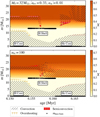 |
Fig. 5. Kippenhahn diagram showing at what mass coordinates, m (y-axis), internal mixing regions arise, as well as the hydrogen mass fraction (color coded) as function of time for two 32 M⊙ evolutionary sequences. One is computed with inefficient semiconvective mixing (αsc = 0.01; top panel), and the other one is computed with efficient semiconvective mixing (αsc = 100; bottom panel). The displayed time interval starts near core hydrogen exhaustion and ends in the early stage of core helium burning. The overshooting parameter for both models is αov = 0.33, and rotation is not included. Black dots indicate the mass coordinate of the maximum specific nuclear energy generation. |
On the other hand, when semiconvective mixing is efficient (bottom panel of Fig. 5, αsc = 100) H/He gradients around mass coordinate m = 15…20 M⊙ can quickly wash out. As a result, the criterion for semiconvection

is no longer fulfilled. In the equation above, ∇ad is the adiabatic temperature gradient (d log T/d log P)ad, ∇rad is the radiative temperature gradient, and ∇μ is the mean molecular weight gradient. Here, f is defined as f = −χμ/χT, where χμ = (d log P/d log μ)ρ, T and χT = (d log P/d log T)ρ, μ. Convection occurs in these layers after ∇μ has vanished. As a consequence of rapid semiconvective mixing, hydrogen-rich material is pushed close to the hydrogen-depleted core, thereby steepening the H/He gradient dX/dQ.
The top panel of Fig. 6 shows dX/dQ as a function of stellar radius R for models computed with various semiconvective efficiencies and a fixed overshooting parameter (αov = 0.33). In sequences with the most efficient semiconvection (αsc = 10, 100) the H/He gradient starts to increase immediately when the star expands after the MS. In contrast, the model sequences with less efficient semiconvection (αsc = 0.01, 0.1, 1) experience no noticeable change in their hydrogen profile immediately after the MS. During core helium burning, the H/He gradient only increases slightly as the innermost hydrogen layers are converted into helium.
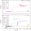 |
Fig. 6. H/He gradient dX/dQ (cf. Fig. 1 in Sect. 2) as a function of stellar radius for 32 M⊙ sequences computed with various assumptions on internal mixing. Thick solid lines indicate core hydrogen burning and thin solid lines indicate core helium burning. The short-lived in-between phase is displayed with a dashed line. In the top panel, αov = 0.33 is adopted in all models while αsc is varied. In the bottom panel, all models are computed with αsc = 1 while αov is varied. |
3.2.2. The role of overshooting
Similar to in Sect. 3.2.1, we explore here how the efficiency of overshooting affects the evolution of the radius R and the H/He gradient dX/dQ. For this, we fix the semiconvection parameter to αsc = 1. The bottom panel of Fig. 6 shows two effects of an increasing αov on MS stars. First, dX/dQ becomes slightly larger (∼3 instead of ∼2), but not close to the dX/dQ values of ∼10 or higher that are required to explain the properties of the apparently single WR stars in the SMC (according to Schootemeijer & Langer 2018). Second, the stars can reach larger radii at the end of the MS. In the model sequence without overshooting, some semiconvective mixing can already occur during the MS, which causes a slight increase in dX/dQ.
A third effect of overshooting manifests itself after the MS evolution. In model sequences with large αov values, steep H/He gradients of dX/dQ > 10 do not develop. Overshooting plays a role here because it changes the shape of the hydrogen profile, which determines if and where the superadiabatic layers (i.e., where ∇rad > ∇ad, see Eq. 1) form that are required for semiconvective mixing. As found by Langer (1991), such layers are less likely to form in models with larger overshooting, and as a result, less semiconvective mixing takes place in these models.
This shows that overshooting has a strong effect on the amount of semiconvective mixing that takes place after core hydrogen exhaustion. Therefore, we consider the simultaneous variation of both mixing processes in the following section.
3.2.3. Semiconvection and overshooting
Here, we consider the same model grids as displayed in Fig. 4. Apart from the question of whether or not models produce steep H/He gradients, we also want to answer the question pertaining to when this might happen. This is especially important in the context of binary interaction. Defining (Δlog R)tot as the total increase in log R (R is in Solar units here) from the ZAMS to the maximum stellar radius, we consider which part of this increase occurs while the H/He gradient fulfills the criterion dX/dQ > 10: (Δ log R)dX/dQ > 10. For example, the αsc = 100 model sequence shown in the top panel of Fig. 6 has a value of (Δ log R)dX/dQ > 10/(Δ log(R)tot ≈ 0.73.
Figure 7 shows that the majority of model sequences either never develop a steep H/He gradient (blue pixels) – this is the case for practically all models with αsc ≤ 0.3 as well as for almost all models with αov ≥ 0.44 – or they do so rather early during their post-MS expansion (orange/red pixels). Only a few sequences show intermediate behavior.
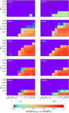 |
Fig. 7. As in Fig. 4, but now the color-coding indicates during which fraction of the overall radius growth of a given sequence ((Δ log R)tot) the internal H/He gradient dX/dQ exceeded a value of 10. Blue color indicates models in which the H/He gradient remains shallow, while red color indicates models where a steep H/He gradient is established early on. |
Only the models with the lowest-shown initial masses (12 M⊙ and 16 M⊙) behave significantly differently from what is described above. None of these are able to produce H/He gradients of dX/dQ > 10 before core helium ignition. In some model sequences (for αsc ≥ 1 and αov ≤ 0.11) such steep H/He gradients are reached during core helium burning, after the star has already significantly expanded – therefore, they represent an intermediate case.
The derived minimum initial mass of the hot SMC WR stars is ∼40 M⊙ (Hainich et al. 2015; Shenar et al. 2016; Schootemeijer & Langer 2018). In this mass range, Fig. 7 shows that to create steep H/He gradients inferred for SMC WR stars, the semiconvection efficiency needs to be of the order of unity or larger. In addition, overshooting cannot exceed 0.33 pressure scale heights; in cases where their progenitors are born with 50 M⊙ or more, this number is reduced to 0.22.
We find that the parameter space described above, where model sequences develop steep H/He gradients, is strongly correlated with the parameter space where model sequences spend at least a significant fraction of their helium-burning lifetime as objects hotter than RSGs (Sect. 3.1.2). This shows that the occurrence of the post-MS BSG phenomenon is tightly linked to internal mixing.
3.2.4. Rotational mixing
Rotation is predicted to drive mixing processes in the envelopes of rapidly spinning stars (e.g., Maeder 1987; Langer 1992). As a result, these processes might have a non-negligible effect on the shape of the hydrogen profiles that we investigate. Therefore, we simulate a number of rotating model sequences to explore to what extent rotational mixing alters the hydrogen profile of our models.
In Fig. 8, we show the hydrogen profile of two sets of six models that are close to core hydrogen exhaustion (Xc = 0.01). These 32 M⊙ birth mass models have initial rotation velocities of vrot, i = 0, 75, …, 375 km s−1, and are computed with an overshooting parameter of either αov = 0.11 (top) or αov = 0.33 (bottom). The hydrogen profiles for the same value of overshooting are very similar. A modest difference emerges only for the highest considered rotation velocity, vrot, i = 375 km s−1.
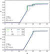 |
Fig. 8. Hydrogen profiles of evolutionary models close to core hydrogen exhaustion, for six different initial rotation velocities (given in km s−1 in the legend). Top panel: evolutionary models computed with an overshooting parameter of αov = 0.11, while αov = 0.33 for the models shown in the bottom panel. |
O-type stars rotating with velocities of 375 km s−1 appear to be rare in the SMC. A study of 31 stars in the SMC cluster NGC 346 by Mokiem et al. (2006) shows that less than one in five stars has a projected rotational velocity above v sin i > 200 km s−1. Furthermore, extreme rotators are predicted to evolve quasi-chemically homogeneously (e.g., Yoon & Langer 2005; Brott et al. 2011), in which case no sizable H/He gradient is expected. In conclusion, rotational mixing as implemented in our models does not appear to be a major factor in determining the shape of the chemical profile for the majority of stars, and therefore it cannot be expected to be a major factor in both the formation of steep H/He gradients and in post-MS evolution. To illustrate the latter point, Fig. A.2 in Appendix A compares HRDs in which the evolutionary models have different initial rotation velocities. However, we remind the reader that rotational mixing depends on a number of uncertain physics assumptions (Lau et al. 2014) and evolutionary models that include stronger shear mixing, for example, might show different behavior. We discuss these models in Sect. 4.
4. Comparison with earlier work
Many of our physics assumptions are similar to the ones used by Brott et al. (2011), who adopted a semiconvection parameter of αsc = 1, and who calibrated the overshooting parameter based on data from the FLAMES Survey of Massive Stars (Hunter et al. 2008a) for stars of 16 M⊙, for which they found αov = 0.335. Unsurprisingly, the post-MS evolution of these models and ours with the same αsc and αov = 0.33 is very similar – both promptly ascend the red giant branch (RGB) and do not experience blue loops. Also, in both sets of models, the smallest initial mass for which the TAMS bends to the coolest effective temperatures due to envelope inflation near the Eddington limit (Sanyal et al. 2015) is about 60 M⊙.
Often in previous evolutionary calculations of massive star models, the Schwarzschild criterion has been adopted for convection. This assumption implies that stabilizing mean molecular weight gradients are not taken into account, which is equivalent to semiconvection leading to mixing as efficient as convection. Therefore, such evolutionary models might behave similarly to our models for which we have used the largest semiconvective efficiency, that is, αsc = 300. For example, Charbonnel et al. (1993) and Meynet et al. (1994) published models using the Schwarzschild criterion in combination with an overshooting parameter of αov = 0.2. Georgy et al. (2013) produced similar models, but adopted αov = 0.1. Below we compare the post-MS evolution of their low-metallicity models with our results.
We find that the post-MS radius evolution of our αsc = 300 (and 100), αov = 0.22 models is indeed similar to that of the αov = 0.2 models of Charbonnel et al. (1993) and Meynet et al. (1994). In both cases, model sequences with initial masses up to 15 − 16 M⊙ can become RSGs during core helium burning. This corresponds to an RSG upper luminosity of log(L/L⊙) = 5.0. More massive models, at least up to 30 − 40 M⊙, never reach RSG temperatures, or only in the very final moments of core helium burning.
Georgy et al. (2013) provide model sequences (αov = 0.1) with and without rotation. Similar to what we describe above, the general behavior of the nonrotating models is very similar to that of our αsc = 300, αov = 0.11 model sequences.
A comparison of models including rotation is more difficult, as different implementations of the angular momentum and chemical transport processes are used in different groups. A treatment of rotation very similar to Heger et al. (2005) and Suijs et al. (2008) is implemented in the MESA code (Paxton et al. 2013): angular momentum is transported by magnetic fields as suggested by Spruit (2002). As a consequence, our models retain close to rigid rotation during their MS evolution, making Eddington-Sweet circulations the dominant mixing process. As we show above, except for a slight reduction of the slope of the H/He gradient, the effects of rotational mixing remain rather limited unless very fast rotation is considered.
Georgy et al. (2013), Chieffi & Limongi (2013), and Limongi & Chieffi (2018) neglect magnetic fields. In their models, the shear instability dominates the transport of elements in radiative zones of the stellar models. Georgy et al. (2013), Choi et al. (2016), Markova et al. (2018), and Limongi & Chieffi (2018) compare such models with those of Brott et al. (2011) for Galactic metallicity, and find that more helium is mixed out of the core into the hydrogen-rich envelope in this case. As a consequence, larger helium cores are produced, similar to the effect of convective core overshooting, as well as shallower H/He gradients. The finding by Georgy et al. (2013) that their rotating and nonrotating models at Z = 0.002 remain BSGs during essentially all of the core helium burning phase (see their Fig. 14) is consistent with the behavior that is expected given their choice of αov = 0.1 and the Schwarzschild criterion for convection. The nonrotating models of Limongi & Chieffi (2018) produce mostly RSGs (for [Fe/H]≥ − 1, except at the highest masses), as they employ the Ledoux criterion and inefficient semiconvection. With increasing rotation, the fraction of their models spent in the BSG regime appears to increase in the mass range 15…25 M⊙ (cf., their Fig. 14), in line with the additional rotational mixing in semiconvection zones mimicking a larger semiconvective mixing efficiency.
While our analysis of the literature results must remain tentative, it does support the general idea that the core mass and the H/He-gradient at the core-envelope interface are the dominant factors in determining the post-MS radius evolution of massive stars. This underlines the view that our results are meaningful beyond the particular parametrization of the individual mixing process chosen for the models of our new stellar-evolution grids.
5. Observational constraints
Above, we describe in which way the various considered internal mixing processes affect the observable stellar properties, that is, the evolution of the models in the HRD and the H/He gradient. In this section, we attempt to find observational constraints which allow us to rule out certain classes of models, and thereby constrain the efficiency of the internal mixing processes.
5.1. Main sequence stars
The occurrence of semiconvection during the MS evolution of massive stars has been studied by Chiosi & Summa (1970); Chiosi et al. (1978), and Langer et al. (1985), for example, who showed that while semiconvection can occur prominently, the evolution of the models during this stage is barely affected by the choice of the semiconvective mixing efficiency. Therefore, we concentrate here on the discussion of the effect of convective core overshooting, whose main effect is to move the location of the TAMS to cooler effective temperatures in the HRD (e.g., Prantzos et al. 1986; Maeder & Meynet 1988; Stothers & Chin 1992).
Finding valid constraints on convective overshooting for massive stars has proven difficult, since the isochrone method used for low- and intermediate-mass stars (Maeder & Meynet 1991) cannot be used due to a lack of populous young star clusters. Brott et al. (2011) used the distribution of rotational velocities to conclude that around 16 M⊙, the overshooting parameter should be close to αov = 0.33.
By studying all the Galactic massive stars for which parameters have been determined through a detailed model atmosphere analysis, Castro et al. (2014) were able to compare their observable parameters with the predictions of stellar-evolution models. They confirmed a value of αov = 0.33 near 16 M⊙ from their data, but found that smaller values would be preferred for smaller initial masses, and larger ones for higher masses. Using their result, Grin et al. (in prep.) found that the best fit to the empirical TAMS of Castro et al. (2014) is obtained for an increasing overshooting with mass such that αov = 0.2 at 8 M⊙ up to αov = 0.5 at 20 M⊙, with a constant value for higher masses.
In a recent study, Castro et al. (2018) analyzed the population of SMC OB field stars as observed within the RIOTS4 survey (Lamb et al. 2016). They derived a tentative TAMS, which agrees well with the one from the Brott et al. (2011) SMC models using αov = 0.335, while also finding some hints of a mass dependence. We conclude that for the considered mass range values of the overshooting parameter of the order of αov = 0.3 seem to provide the best match to observations of massive MS stars.
5.2. Red supergiants
Both Levesque et al. (2006) and Davies et al. (2013) show that the SMC RSG population extends up to a luminosity of log(L/L⊙) ≈ 5.3 − 5.4 but not beyond. Earlier studies (e.g., Massey & Olsen 2003) reported a higher luminosity cut-off. However, the inferred temperatures have since been revised upwards, resulting in smaller bolometric corrections and hence lower luminosities. The most recent investigation of RSGs in the SMC by Davies et al. (2018), who integrated photometric fluxes over a wide wavelength range to obtain the luminosity, also found a cutoff around log(L/L⊙) ≈ 5.4. The latter study used a large sample of ∼150 RSGs with log(L/L⊙) > 4.7).
In Fig. 9, we compare the RSG luminosity distribution of Davies et al. (2018) to our theoretical predictions for different αsc and αov combinations. To obtain the theoretical predictions, we adopt a constant star formation rate and a Salpeter initial mass function (Salpeter 1955). We further assume that there are 300 core helium burning stars in the SMC with log(L/L⊙) > 4.7. We obtain this number by adding the number of 150 BSGs (see Sect. 5.3) in this luminosity range to the 150 RSGs in the sample of Davies et al. (2018). Although uncertain, we expect this to match the true number of stars to within at least a factor of a few, as it could be lower due to foreground contamination, or higher due to incompleteness of the sample, in particular for the BSGs. With this uncertainty in mind, the predicted distributions in Fig. 9 could still be a good fit to the observations even if they would need to be scaled up or down by some amount. To be consistent with Davies et al. (2018), we make the division between RSGs and hotter objects at 7 kK.
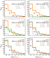 |
Fig. 9. Diagrams showing the predicted luminosity distribution of red supergiants in the SMC. Each of the six diagrams has a different value for the overshooting parameter αov. The red diamonds indicate the number of red supergiants observed by Davies et al. (2018). |
Figure 9 shows that the largest discrepancy between the observed RSG luminosity distribution and the predictions occurs for efficient semiconvection and the lowest overshooting, where hardly any RSGs are produced (see also Fig. 4). There, the RSG number fraction fRSG = NRSG/(NRSG + NBSG) is only a few per cent, which would imply that about 1500–5000 BSGs would need to be present in the SMC given that 150 RSGs are observed. Such a large BSG population would rival the entire SMC in terms of stellar luminosity (which is about 4 × 10⁸ L⊙; Bekki & Stanimirović 2009). Davies et al. (2018) compare with tracks of Georgy et al. (2013) where the Schwarzschild criterion for convection (which translates into extremely efficient semiconvection) and αov = 0.1 are assumed. Indeed, when we trace the progenitor evolution of the RSG models that were considered we find that ∼5000 BSGs should be present to obtain 150 RSGs, based on the corresponding lifetimes of the models of Georgy et al. (2013).
In model sequences where little semiconvective mixing occurs (i.e., where αsc is low and/or αov is high), the mismatch in Fig. 9 between observations and model predictions is less striking. Up to log(L/L⊙) = 5.3, the observed steepness of the drop of the number of RSGs with increasing luminosity could reflect a combination of the initial mass function and the shorter lifetime of heavier helium cores. This drop can be well matched by the model sequences that burn helium as RSGs. However, for luminosities of log(L/L⊙) > 5.3, essentially no RSGs are observed (Davies et al. list one RSG at log(L/L⊙) ≃ 5.4, and one more at log(L/L⊙) ≃ 5.6), while grids of models where little semiconvective mixing occurs predict some tens of RSGs.
There is a limited range of mixing parameters that might be compatible with the observed paucity of luminous RSGs. We see in Fig. 4 that in the mass range from 12 to 25 M⊙, for efficient semiconvection the pure BSG solutions tend to prevail more often when the mass increases. Therefore, if nature had chosen for convective core masses corresponding to, for example, αov = 0.22 and αsc = 100, there would be a gap in the luminosity distribution of RSGs, because stars with initial masses of 20 M⊙ and above would never become RSGs. Figure A.1 shows several such luminosity gaps for low overshooting and high semiconvection parameters, and Fig. A.2 shows that these gaps also prevail in our models which include rotational mixing. Such gaps could therefore explain the observed scarcity of luminous RSGs with masses of the order of 25 − 32 M⊙. In this case the upper RSG luminosity limit would not be set by strong RSG winds stripping off the hydrogen envelopes in more luminous stars. Instead, it would be set by the helium burning stars around the upper luminosity limit being more likely to be BSGs.
In most of our grids, we find models above ∼40 M⊙ (log(L/L⊙) ≃ 5.7) to evolve to low effective temperatures, even though they remain hotter than classical RSGs. The fact that in these cases such objects are predicted (together, the two log(L/L⊙)≥5.7 bins in Fig. 9 typically contain of the order of 15–20 objects) but none are observed could have something to do with uncertainties in mass-loss rates for the brightest cool stars (as discussed by Davies et al. 2018). This may also be prone to the uncertain effect of envelope inflation (Sanyal et al. 2017). Alternatively, stars this massive could simply happen to be rare in the SMC for a reason that is not yet fully understood (as indicated by the results of Blaha & Humphreys 1989).
It remains remarkable that the range in mixing parameters which offers a tentative solution of the RSG luminosity problem described in Davies et al. (2018) has a significant overlap with the parameter ranges favored by other observational constraints.
5.3. Blue supergiants
The shape and size of the BSG population in the SMC appears to be more uncertain than that of the RSG population. For our analysis, we combine the two samples of approximately 100 A-type supergiants from Humphreys et al. (1991) and about 50 B-type supergiants of Kalari et al. (2018). This number is comparable to the number of RSGs; as a result, the blue-to-red supergiant ratio (b/r ratio) is then of the order of unity. These samples cover the entire temperature range of BSGs, and we consider the same luminosity range as for RSGs (Sect. 5.2). However, observational studies presented by Blaha & Humphreys (1989) and Evans et al. (2006) also contain some tens of objects in the BSG temperature range – thus, depending on the amount of overlap and other biases, the above number of BSGs could be seen as a lower limit.
Figure 10 shows that in synthetic populations where efficient semiconvective mixing does not take place (e.g., if αsc = 0.01 or αov ≥ 0.44), the BSG population is negligible. This means that the predicted b/r ratio is close to zero, which seems to be at odds with aforementioned observations. For the opposite case, for example where αsc = 100 and αov < 0.22, almost all helium burning stars are predicted to be BSGs, resulting in a b/r ratio much larger than unity. Given the uncertainties described above, this evolutionary scenario could still agree with the observed BSG population, however it is clearly challenged by the presence of the observed RSG population (Sect. 5.2). For constant overshooting, we conclude that the synthetic population with αsc ≈ 100 and αov = 0.33 performs best in simultaneously explaining the RSG and BSG populations in the SMC. In this case, a b/r ratio of the order of one is predicted (162 RSGs per 138 BSGs; see Figs. 9 and 10). Most other combinations of efficiencies predict either a very low or very high b/r ratio.
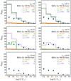 |
Fig. 10. As in Fig. 9, but this diagram is showing the luminosity distribution of blue supergiants. Here, blue diamonds indicate the combined number of blue supergiants observed in the SMC by Humphreys et al. (1991) and Kalari et al. (2018). |
While these values might provide the most satisfying match between observations and theory, there could be a mismatch at luminosities below the range that we discussed above. The evolutionary sequences with Mini = 12 M⊙ and below do not experience blue loops for these values, while some A- and B-type supergiants are observed in the associated luminosity range. We note that for these relatively faint stars, detection biases are larger. A possible explanation is that the extent of overshooting is lower at lower initial masses, as proposed by Castro et al. (2014) and Grin et al. (in prep. – see also Sect. 5.1). If that is the case, stars with lower initial masses also become BSGs (Fig. 2 and A.1). Alternatively, these objects could have a binary origin – we discuss this in Sect. 6. A more complete observational picture is required in order to draw any robust conclusions.
5.4. Surface abundances
The nitrogen abundance at the surface of a star can be used as a probe for its evolutionary history. We illustrate this in Fig. 11. For stars that are approaching the RGB from hotter temperatures, no nitrogen enhancements are predicted by our evolutionary sequences in the nonrotating case (shown in the left panel). However, for stars that are on a blue loop excursion, it is predicted that CNO-processed material is dredged up from their deep convective envelopes during the prior RSG phase. As a result, the mass fractions of helium and nitrogen at the surface are enhanced. This applies to the light blue diamonds in Fig. 11 (left) around log(L/L⊙) = 5 and log(Teff/K) = 4.2. The evolutionary tracks that we show are those where αsc = 100 and αov = 0.33, which could best explain the RSG and BSG populations.
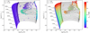 |
Fig. 11. Hertzsprung–Russell diagram showing the nitrogen surface mass fraction of our evolutionary sequences with αsc = 100 and αsc = 0.33. The initial masses of the shown stellar tracks are evenly logarithmically spaced every 0.02 dex. Similarly to Fig. 2, a marker indicates a 50 000 yr time step, a circle indicates core hydrogen burning, and a diamond indicates core helium burning. Left: model sequences are nonrotating. Right: model sequences have an initial rotation velocity of 300 km s−1. |
When rotation is taken into account, stars that have not developed deep convective envelopes can also be enriched in nitrogen. This is illustrated in the right panel of Fig. 11, which shows evolutionary models with an initial rotation velocity of 300 km s−1. Still, stars that are on a blue loop excursion are more enriched in nitrogen because an additional mechanism is at work. These are the orange diamonds around log(L/L⊙) = 5 and log(Teff/K) = 4.2 in the right panel of Fig. 11.
In practice, using nitrogen abundances to constrain the evolutionary history of stars is difficult, because even on the MS a large fraction of stars show nitrogen enrichment (Hunter et al. 2008b; Bouret et al. 2013; Grin et al. 2017), and the observed nitrogen enrichment does not, or at least not clearly, correlate with rotation velocity. Nevertheless, as shown in Fig. 11, also in the case with rotational mixing included, the BSGs that previously underwent an RSG dredge-up phase are significantly more enriched in nitrogen than those that did not. A comprehensive view of the nitrogen abundances of the SMC supergiants would therefore constitute a thorough test of our models.
The nine A-type stars in the SMC analyzed by Venn (1999) indeed show nitrogen enrichment, varying from weak to strong. Because they all have luminosities below log(L/L⊙) ≈ 5, this is in agreement with our predictions shown in Fig. 11 although less scatter would be expected.
5.5. The most massive stars
So far we have paid relatively little attention to the predictions of our models for the most luminous stars. The reason for this is that such stars are expected to be quite rare, and there are very few solid observational constraints available at this time. In addition, although the SMC offers the advantage of smaller mass-loss-rate uncertainties, this is no longer the case if we consider initial stellar masses of 60 M⊙ and higher. Additionally, even in the SMC, such very massive stars are very close to the Eddington limit, such that envelope inflation may strongly affect their radii and effective temperatures. Therefore, even when picking the model grid with the most promising mixing parameters, the models for the highest masses are the least likely to be close to reality.
An exception is perhaps the core hydrogen burning phase of evolution, for which the mass-loss rates are the best understood. In this respect, our prediction that the TAMS bends to very cool temperatures at luminosities below log(L/L⊙) ≈ 6 appears to be relatively robust, at least for what we identified as the most likely mixing parameters: efficient semiconvection and intermediate overshooting. As shown in Figs. 2 and A.1, this leads to a continuous effective temperature distribution of the most luminous stars, rather than showing a pronounced post-MS gap as visible in the grids computed with the smallest overshooting parameters. We note that Castro et al. (2018) find tentative evidence for this; however the interpretation of their data is still somewhat ambiguous.
Finally, we want to point out that with the mass-loss rate assumptions adopted for our models, which are state-of-the-art but are surely uncertain at low effective temperatures, there are essentially no hydrogen-poor or hot WR stars produced independent of our assumptions on internal mixing.
6. Discussion
6.1. Summarizing our results
In the sections above, we calculated the systematic trends that occur in massive star evolution models with an SMC initial chemical composition as a function of the efficiency of internal mixing processes. We saw that these mixing processes determine the core mass increase and the slope of the H/He-gradient at the core–envelope interface, which are the internal structure parameters ruling the evolution of the stars in the HRD.
We then confronted these evolutionary models with various observational constraints, and found that for the overshooting parameter αov (which determines the increase of the core masses) and the semiconvection parameter αsc (which is the key parameter for determining the H/He gradient) only a limited range of combinations is compatible with those observational constraints.
We have seen that the constraints on the MS imply convective core overshooting of the order of αov = 0.33 in the considered mass range. Interestingly, larger overshooting has the consequence that the stellar tracks produce essentially no BSGs with luminosities of log(L/L⊙) ≲ 5.5 and temperatures log(Teff/K) ≲ 4.3 (cf., Fig. A.1). Since numerous stars that fit this description are observed in the SMC (e.g., Blaha & Humphreys 1989), an overshooting parameter of αov significantly above 0.33 seems to be excluded. This provides an independent constraint on the overshooting parameter, in addition to those derived from the width of the MS. When the requirement of a large H/He-gradient from Schootemeijer & Langer (2018) is taken into account, such large overshooting is ruled out once more. Similarly, αov = 0…0.11 yields only BSGs for a wide range of initial masses for models where semiconvection is reasonably efficient. As a result, almost no RSGs are then predicted to exist in the luminosity range where Davies et al. (2018) report 150 of these objects.
Conversely, Fig. A.1 shows that inefficient semiconvection (αsc < 1) can be ruled out, because – independent of the amount of overshooting – far too few BSGs are produced. Again, this conclusion is reinforced by the fact that αsc < 1 does not allow for steep H/He-gradients. In fact, the almost complete overlap in the parameter space of only shallow H/He-gradients (Fig. 7) with the parameter space where only RSGs are produced (Fig. 4) reinforces the conclusion of Schootemeijer & Langer (2018) that steep H/He-gradients are observationally required and generalizes it to a wider mass range. Finally, we saw in Sect. 5.2 that the parameter range that can at least partially explain the problem of the paucity of luminous RSGs falls within the range that is compatible with all other observational constraints.
The situation is summarized in Fig. 12. We see that the parameter subspace where all observational tests are passed is rather small. In fact, the overshooting parameter seems to be well constrained to the interval 0.2 ≲ αov ≲ 0.35. Semiconvection, on the other hand, is required to be efficient in the sense that αsc > 1. Here it should be mentioned that the allowed parameter space for the semiconvection parameter may appear larger than it is, since for αsc ≳ 10 our models show very similar behavior.
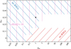 |
Fig. 12. Schematic diagram indicating which part of the αsc and αov parameter space is at odds with our three different criteria. These criteria are (1) the ability to produce steep H/He gradients (Sect. 3.2, purple vertical lines), (2) for stars with log(L/L⊙) ≲ 5.5 to spend part of core helium burning as blue supergiants (blue diagonal lines), (3) for stars with log(L/L⊙)≥4.7 during core helium burning to become red supergiants (red diagonal lines). |
Importantly, Fig. 12 shows the existence of a subspace of the considered parameter space that appears to be compatible with all observational constraints. We note that a priori there was no guarantee of this outcome, which offers hope that our problem is well posed – in the sense that the adopted physical descriptions allow for a representation of the real stars – despite the caveats discussed below. Further tests may show whether or not this turns out to be an illusion. For example, a study similar to this one needs to be done for Galactic and LMC composition, although the higher metallicity of these environments may introduce additional uncertainties through the increased importance of stellar winds. The concept of this work may also be applicable to intermediate-mass stars, however it is already clear that consideration of a mass dependence for the mixing parameters cannot be avoided in this case (see below).
6.2. Caveats
Figure 12 gives an overview of our findings, without subdividing the mass range we consider (9…100 M⊙). However, in the discussion above, we already had to specify smaller initial mass ranges when discussing specific observational constraints. Indeed, the physical situation in our models changes significantly: our 9 M⊙ models are dominated by ideal gas pressure, while radiation pressure is more important in our 100 M⊙ models.
In fact, when considering the overshooting parameter, it already appears evident that (in the way it is currently parametrized) it cannot be constant for all core hydrogen burning stars. For intermediate- and low-mass stars, good constraints exist pointing to values of αov ≲ 0.2 (e.g., Aerts 2013; Claret & Torres 2016). On the other hand, the results of Castro et al. (2014) argue for an increase of αov with mass (Grin et al., in prep.). Furthermore, as discussed in Sect. 5.3, a lower overshooting than indicated by Fig. 12 may yield better agreement with the blue-to-red supergiant ratio at the lowest considered masses.
Such a mass dependence would actually not be surprising, since αov is an ad hoc parameter, which is not backed up by any physical theory. The treatment of semiconvection on the other hand is based on a local, linear stability analysis (Kato 1966; Langer et al. 1983), which fully accounts for a mixture of gas and radiation pressure. Therefore, we may hope that the mass dependence of this parameter is weaker or absent.
Furthermore, our discussion of the chemical structure of massive stars remained limited, since we only considered the parameters core mass and H/He gradient. Clearly (as also indicated by Fig. 8), hydrogen and helium profiles can be quite complex and may need more than two parameters to describe them. The inclusion of additional parameters would nevertheless be difficult at the moment, and their requirement has not yet been shown; the convergence of the viable part of the parameter space from multiple constraints does not support a requirement.
On the other hand, we know that even for a fixed initial chemical composition, the initial stellar mass is not the only parameter describing its future evolution. Rotation and binarity are widely discussed as initial parameters affecting the evolution of massive stars (Maeder & Meynet 2012; Langer 2012). However, while for massive stars living in a binary is the rule rather than the exception (Sana et al. 2012), the fraction of isolated massive stars whose evolution is significantly affected by rotation is unclear. As discussed in Sect. 3, we find the effects of rotation on our models to be quite limited – except for extreme rotation, which allows for chemically homogeneous evolution (Yoon et al. 2006; Brott et al. 2011), but this is thought to be very rare. However, in the framework of models which allow for a significant redistribution of hydrogen and helium for average rotation rates (cf., Sect. 3), rotation would need to be considered as an important third parameter.
Our neglect of binarity however, is harder to justify, except for feasibility reasons. The two additional necessary initial parameters (initial secondary mass, and initial separation) tremendously expand the initial parameter space to consider. However, now that our analysis of single star models has narrowed the viable parameter space for the mixing parameters, our next step will be to compute binary evolution grids with the current best guess for these, and investigate whether or not binarity affects our conclusions.
While binarity may be omnipresent in massive stars, this does not specifically imply that it is important for our discussion. Considering MS stars, of the order of 10% and 15% may be merger products or mass gainers in post-mass-transfer systems, respectively (de Mink et al. 2014). However, if these were to be fully rejuvenated, they might be relatively indistinguishable from ordinary single stars and may continue their evolution as such. In fact, the very efficient semiconvective mixing advocated by our results would imply that rejuvenation occurs in the vast majority of cases (Braun & Langer 1995). On the other hand, it has been suggested that stellar mergers produce strong magnetic fields (Ferrario et al. 2009; Langer 2012; Schneider et al. 2016), in which case the evolution on the MS and beyond could be strongly affected (Petermann et al. 2015). As about 7% of the massive MS stars are found to be magnetic (Fossati et al. 2015; Grunhut et al. 2017), this may affect our analysis at this level.
The only other branch of massive binary evolution that may be of relevance here (because, e.g., common envelope evolution or binaries involving compact objects produce exotic, easily identifiable types of stars) are post-MS stellar mergers. Such mergers produce stars whose core mass is smaller compared to that of a single star of the same mass. Such objects are known to spend nearly all of core helium burning as BSGs (Braun & Langer 1995; Justham et al. 2014). The fraction of massive binaries that produce such stars is again estimated to be of the order of 10% (Podsiadlowski et al. 1992); however, the uncertainty of this number is considerable (de Mink et al. 2014) and not independent of the mixing parameters discussed here.
In summary, much more work is needed to consolidate or modify our conclusion. However, at present it is reassuring that many constraints seem to point in the same direction.
7. Conclusions
In this study, we computed a large number of grids of massive star model sequences to comprehensively analyze the effects of the most relevant internal mixing processes on MS and post-MS evolution. We chose to focus on models with an SMC initial chemical composition, such that uncertain mass-loss rates affect our conclusions as little as possible.
We compared the predictions of our models to a multitude of observational constraints in the SMC. These included the observed widths of the MS band in the HRD, the presence of both blue and red supergiants for a considerable range of luminosities, the empirical upper luminosity limit of red supergiants, and the requirement of a steep H/He-gradient at the core–envelope interface in the hot hydrogen-rich Wolf-Rayet stars.
As summarized in Sect. 6.1 and Fig. 12, we find a small and well-defined subspace of the mixing parameters where all constraints can be satisfied simultaneously. Conversely, we can exclude most of the considered parameter space. In terms of the formulation of the mixing processes used in our models, we find that semiconvective mixing needs to be efficient (αsc ≳ 1), while convective core overshooting is restricted to intermediate values (0.22 ≲ αov ≲ 0.33) for most of the considered mass range, with possibly smaller values favored below ∼10 M⊙. Rotational mixing in our models was found to be of limited importance.
In terms of structural parameters, which are relevant beyond our chosen mathematical formulation of the mixing processes, we find a necessity for a moderate core mass increase over the canonical value, which may be produced by convective core overshooting or otherwise, and a H/He-gradient which is at least five times steeper than that emerging naturally from the retreating convective core during core hydrogen burning. While this steep H/He gradient has been found previously for stars above ∼40 M⊙, we find it to be valid for stars down to ∼9 M⊙.
Since our results could only be derived with various caveats (cf. Sect. 6.2), more theoretical work is needed to consolidate them, in particular to include models of close binary evolution. In any case, much more stringent tests of our results will be enabled by a complete set of spectroscopic data of the massive stars in this key galaxy, the SMC, where currently available data remain fragmentary.
References
- Aerts, C. 2013, in EAS Publ. Ser., eds. K. Pavlovski, A. Tkachenko, & G. Torres, 64, 323 [Google Scholar]
- Alongi, M., Bertelli, G., Bressan, A., et al. 1993, A&AS, 97, 851 [NASA ADS] [Google Scholar]
- Bekki, K., & Stanimirović, S. 2009, MNRAS, 395, 342 [NASA ADS] [CrossRef] [Google Scholar]
- Belczynski, K., Dominik, M., Bulik, T., et al. 2010, ApJ, 715, L138 [NASA ADS] [CrossRef] [Google Scholar]
- Blaha, C., & Humphreys, R. M. 1989, AJ, 98, 1598 [NASA ADS] [CrossRef] [Google Scholar]
- Böhm-Vitense, E. 1958, ZAp, 46, 108 [NASA ADS] [Google Scholar]
- Bouret, J.-C., Lanz, T., Martins, F., et al. 2013, A&A, 555, A1 [NASA ADS] [CrossRef] [EDP Sciences] [Google Scholar]
- Braun, H., & Langer, N. 1995, A&A, 297, 483 [NASA ADS] [Google Scholar]
- Brott, I., de Mink, S. E., Cantiello, M., et al. 2011, A&A, 530, A115 [NASA ADS] [CrossRef] [EDP Sciences] [Google Scholar]
- Canuto, V. M. 1999, ApJ, 518, L119 [NASA ADS] [CrossRef] [Google Scholar]
- Castro, N., Fossati, L., Langer, N., et al. 2014, A&A, 570, L13 [NASA ADS] [CrossRef] [EDP Sciences] [Google Scholar]
- Castro, N., Oey, M. S., Fossati, L., & Langer, N. 2018, ApJ, 868, 57 [NASA ADS] [CrossRef] [Google Scholar]
- Charbonnel, C., Meynet, G., Maeder, A., Schaller, G., & Schaerer, D. 1993, A&AS, 101, 415 [NASA ADS] [Google Scholar]
- Chen, T.-W., Smartt, S. J., Yates, R. M., et al. 2017, MNRAS, 470, 3566 [NASA ADS] [CrossRef] [Google Scholar]
- Chieffi, A., & Limongi, M. 2013, ApJ, 764, 21 [NASA ADS] [CrossRef] [Google Scholar]
- Chiosi, C., & Summa, C. 1970, Ap&SS, 8, 478 [NASA ADS] [CrossRef] [Google Scholar]
- Chiosi, C., Nasi, E., & Sreenivasan, S. R. 1978, A&A, 63, 103 [NASA ADS] [Google Scholar]
- Choi, J., Dotter, A., Conroy, C., et al. 2016, ApJ, 823, 102 [NASA ADS] [CrossRef] [Google Scholar]
- Claret, A., & Torres, G. 2016, A&A, 592, A15 [NASA ADS] [CrossRef] [EDP Sciences] [Google Scholar]
- Cloutman, L. D., & Whitaker, R. W. 1980, ApJ, 237, 900 [NASA ADS] [CrossRef] [Google Scholar]
- Davies, B., Kudritzki, R.-P., Plez, B., et al. 2013, ApJ, 767, 3 [NASA ADS] [CrossRef] [Google Scholar]
- Davies, B., Crowther, P. A., & Beasor, E. R. 2018, MNRAS, 478, 3138 [NASA ADS] [CrossRef] [Google Scholar]
- de Mink, S. E., Sana, H., Langer, N., Izzard, R. G., & Schneider, F. R. N. 2014, ApJ, 782, 7 [NASA ADS] [CrossRef] [Google Scholar]
- Drout, M. R., Massey, P., Meynet, G., Tokarz, S., & Caldwell, N. 2009, ApJ, 703, 441 [NASA ADS] [CrossRef] [Google Scholar]
- Evans, C. J., Lennon, D. J., Smartt, S. J., & Trundle, C. 2006, A&A, 456, 623 [NASA ADS] [CrossRef] [EDP Sciences] [Google Scholar]
- Ferrario, L., Pringle, J. E., Tout, C. A., & Wickramasinghe, D. T. 2009, MNRAS, 400, L71 [NASA ADS] [CrossRef] [Google Scholar]
- Fossati, L., Castro, N., Schöller, M., et al. 2015, A&A, 582, A45 [NASA ADS] [CrossRef] [EDP Sciences] [Google Scholar]
- Georgy, C., Ekström, S., Eggenberger, P., et al. 2013, A&A, 558, A103 [NASA ADS] [CrossRef] [EDP Sciences] [Google Scholar]
- Graham, J. F., & Fruchter, A. S. 2017, ApJ, 834, 170 [NASA ADS] [CrossRef] [Google Scholar]
- Grevesse, N., Noels, A., & Sauval, A. J. 1996, in Cosmic Abundances, eds. S. S. Holt, & G. Sonneborn, ASP Conf. Ser., 99, 117 [NASA ADS] [Google Scholar]
- Grin, N. J., Ramírez-Agudelo, O. H., de Koter, A., et al. 2017, A&A, 600, A82 [NASA ADS] [CrossRef] [EDP Sciences] [Google Scholar]
- Grossman, S. A., & Taam, R. E. 1996, MNRAS, 283, 1165 [NASA ADS] [CrossRef] [Google Scholar]
- Grunhut, J. H., Wade, G. A., Neiner, C., et al. 2017, MNRAS, 465, 2432 [NASA ADS] [CrossRef] [Google Scholar]
- Hainich, R., Pasemann, D., Todt, H., et al. 2015, A&A, 581, A21 [Google Scholar]
- Hamann, W.-R., Koesterke, L., & Wessolowski, U. 1995, A&A, 299, 151 [NASA ADS] [Google Scholar]
- Heger, A., Langer, N., & Woosley, S. E. 2000, ApJ, 528, 368 [NASA ADS] [CrossRef] [Google Scholar]
- Heger, A., Woosley, S. E., & Spruit, H. C. 2005, ApJ, 626, 350 [NASA ADS] [CrossRef] [Google Scholar]
- Hopkins, P. F., Kereš, D., Oñorbe, J., et al. 2014, MNRAS, 445, 581 [NASA ADS] [CrossRef] [Google Scholar]
- Höppner, W., & Weigert, A. 1973, A&A, 25, 99 [NASA ADS] [Google Scholar]
- Humphreys, R. M., Kudritzki, R. P., & Groth, H. G. 1991, A&A, 245, 593 [NASA ADS] [Google Scholar]
- Hunter, I., Lennon, D. J., Dufton, P. L., et al. 2008a, A&A, 479, 541 [NASA ADS] [CrossRef] [EDP Sciences] [Google Scholar]
- Hunter, I., Brott, I., Lennon, D. J., et al. 2008b, ApJ, 676, L29 [NASA ADS] [CrossRef] [Google Scholar]
- Iben, Jr., I. 1993, ApJ, 415, 767 [NASA ADS] [CrossRef] [Google Scholar]
- Justham, S., Podsiadlowski, P., & Vink, J. S. 2014, ApJ, 796, 121 [NASA ADS] [CrossRef] [Google Scholar]
- Kalari, V. M., Vink, J. S., Dufton, P. L., & Fraser, M. 2018, A&A, 618, A17 [NASA ADS] [CrossRef] [EDP Sciences] [Google Scholar]
- Kato, S. 1966, PASJ, 18, 374 [NASA ADS] [Google Scholar]
- Kewley, L., & Kobulnicky, H. A. 2007, Astrophys. Space Sci. Proc., 3, 435 [NASA ADS] [CrossRef] [Google Scholar]
- Köhler, K., Langer, N., de Koter, A., et al. 2015, A&A, 573, A71 [NASA ADS] [CrossRef] [EDP Sciences] [Google Scholar]
- Korn, A. J., Becker, S. R., Gummersbach, C. A., & Wolf, B. 2000, A&A, 353, 655 [NASA ADS] [Google Scholar]
- Lamb, J. B., Oey, M. S., Segura-Cox, D. M., et al. 2016, ApJ, 817, 113 [NASA ADS] [CrossRef] [Google Scholar]
- Langer, N. 1991, A&A, 252, 669 [NASA ADS] [Google Scholar]
- Langer, N. 1992, A&A, 265, L17 [NASA ADS] [Google Scholar]
- Langer, N. 2012, ARA&A, 50, 107 [NASA ADS] [CrossRef] [Google Scholar]
- Langer, N., & Maeder, A. 1995, A&A, 295, 685 [NASA ADS] [Google Scholar]
- Langer, N., Fricke, K. J., & Sugimoto, D. 1983, A&A, 126, 207 [NASA ADS] [Google Scholar]
- Langer, N., El Eid, M. F., & Fricke, K. J. 1985, A&A, 145, 179 [NASA ADS] [Google Scholar]
- Lau, H. H. B., Izzard, R. G., & Schneider, F. R. N. 2014, A&A, 570, A125 [NASA ADS] [CrossRef] [EDP Sciences] [Google Scholar]
- Levesque, E. M., Massey, P., Olsen, K. A. G., et al. 2006, ApJ, 645, 1102 [NASA ADS] [CrossRef] [Google Scholar]
- Limongi, M., & Chieffi, A. 2018, ApJS, 237, 13 [NASA ADS] [CrossRef] [Google Scholar]
- Maeder, A. 1987, A&A, 178, 159 [NASA ADS] [Google Scholar]
- Maeder, A., & Meynet, G. 1988, A&AS, 76, 411 [NASA ADS] [Google Scholar]
- Maeder, A., & Meynet, G. 1991, A&AS, 89, 451 [NASA ADS] [CrossRef] [Google Scholar]
- Maeder, A., & Meynet, G. 2000, A&A, 361, 159 [NASA ADS] [Google Scholar]
- Maeder, A., & Meynet, G. 2012, Rev. Mod. Phys., 84, 25 [NASA ADS] [CrossRef] [Google Scholar]
- Markova, N., Puls, J., & Langer, N. 2018, A&A, 613, A12 [NASA ADS] [CrossRef] [EDP Sciences] [Google Scholar]
- Massey, P., & Olsen, K. A. G. 2003, AJ, 126, 2867 [NASA ADS] [CrossRef] [Google Scholar]
- Merryfield, W. J. 1995, ApJ, 444, 318 [NASA ADS] [CrossRef] [Google Scholar]
- Meynet, G., Maeder, A., Schaller, G., Schaerer, D., & Charbonnel, C. 1994, A&AS, 103, 97 [Google Scholar]
- Mokiem, M. R., de Koter, A., Evans, C. J., et al. 2006, A&A, 456, 1131 [NASA ADS] [CrossRef] [EDP Sciences] [Google Scholar]
- Mokiem, M. R., de Koter, A., Vink, J. S., et al. 2007, A&A, 473, 603 [NASA ADS] [CrossRef] [EDP Sciences] [Google Scholar]
- Nieuwenhuijzen, H., & de Jager, C. 1990, A&A, 231, 134 [NASA ADS] [Google Scholar]
- Paxton, B., Bildsten, L., Dotter, A., et al. 2011, ApJS, 192, 3 [Google Scholar]
- Paxton, B., Cantiello, M., Arras, P., et al. 2013, ApJS, 208, 4 [NASA ADS] [CrossRef] [Google Scholar]
- Paxton, B., Marchant, P., Schwab, J., et al. 2015, ApJS, 220, 15 [Google Scholar]
- Paxton, B., Schwab, J., Bauer, E. B., et al. 2018, ApJS, 234, 34 [NASA ADS] [CrossRef] [EDP Sciences] [Google Scholar]
- Petermann, I., Langer, N., Castro, N., & Fossati, L. 2015, A&A, 584, A54 [NASA ADS] [CrossRef] [EDP Sciences] [Google Scholar]
- Podsiadlowski, P., Joss, P. C., & Hsu, J. J. L. 1992, ApJ, 391, 246 [NASA ADS] [CrossRef] [Google Scholar]
- Prantzos, N., Doom, C., Arnould, M., & de Loore, C. 1986, ApJ, 304, 695 [NASA ADS] [CrossRef] [Google Scholar]
- Renzini, A., Greggio, L., Ritossa, C., & Ferrario, L. 1992, ApJ, 400, 280 [NASA ADS] [CrossRef] [Google Scholar]
- Salpeter, E. E. 1955, ApJ, 121, 161 [Google Scholar]
- Sana, H., de Mink, S. E., de Koter, A., et al. 2012, Science, 337, 444 [Google Scholar]
- Sanyal, D., Grassitelli, L., Langer, N., & Bestenlehner, J. M. 2015, A&A, 580, A20 [NASA ADS] [CrossRef] [EDP Sciences] [Google Scholar]
- Sanyal, D., Langer, N., Szécsi, D. C., Yoon, S., & Grassitelli, L. 2017, A&A, 597, A71 [NASA ADS] [CrossRef] [EDP Sciences] [Google Scholar]
- Schneider, F. R. N., Podsiadlowski, P., Langer, N., Castro, N., & Fossati, L. 2016, MNRAS, 457, 2355 [NASA ADS] [CrossRef] [Google Scholar]
- Schootemeijer, A., & Langer, N. 2018, A&A, 611, A75 [NASA ADS] [CrossRef] [EDP Sciences] [Google Scholar]
- Schulze, S., Krühler, T., Leloudas, G., et al. 2018, MNRAS, 473, 1258 [NASA ADS] [CrossRef] [Google Scholar]
- Shenar, T., Hainich, R., Todt, H., et al. 2016, A&A, 591, A22 [NASA ADS] [CrossRef] [EDP Sciences] [Google Scholar]
- Spruit, H. C. 2002, A&A, 381, 923 [NASA ADS] [CrossRef] [EDP Sciences] [Google Scholar]
- Stancliffe, R. J., Chieffi, A., Lattanzio, J. C., & Church, R. P. 2009, PASA, 26, 203 [NASA ADS] [CrossRef] [Google Scholar]
- Stothers, R. B., & Chin, C.-W. 1992, ApJ, 390, 136 [NASA ADS] [CrossRef] [Google Scholar]
- Sugimoto, D., & Fujimoto, M. Y. 2000, ApJ, 538, 837 [NASA ADS] [CrossRef] [Google Scholar]
- Suijs, M. P. L., Langer, N., Poelarends, A.-J., et al. 2008, A&A, 481, L87 [NASA ADS] [CrossRef] [EDP Sciences] [Google Scholar]
- Venn, K. A. 1999, ApJ, 518, 405 [NASA ADS] [CrossRef] [Google Scholar]
- Vink, J. S., de Koter, A., & Lamers, H. J. G. L. M. 2001, A&A, 369, 574 [NASA ADS] [CrossRef] [EDP Sciences] [Google Scholar]
- Yoon, S.-C., & Langer, N. 2005, A&A, 443, 643 [NASA ADS] [CrossRef] [EDP Sciences] [Google Scholar]
- Yoon, S.-C., Langer, N., & Norman, C. 2006, A&A, 460, 199 [NASA ADS] [CrossRef] [EDP Sciences] [Google Scholar]
- Zaussinger, F., & Spruit, H. C. 2013, A&A, 554, A119 [NASA ADS] [CrossRef] [EDP Sciences] [Google Scholar]
Appendix A: Extra Hertzsprung–Russell diagrams
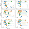 |
Fig. A.2. As in Fig. 2, but now for various αov and initial rotation velocities (indicated in the bottom left of each panel, in units of km s−1). The models were computed with a relatively high time resolution (see Sect. 2) and with αsc = 1. |
All Figures
|
Fig. 1. Various quantities of our 16 M⊙ stellar model computed with αov = 0.11 after core hydrogen depletion as a function of the internal mass coordinate. The model is undergoing hydrogen shell burning, as indicated by the relative rate of nuclear energy production (black dotted line). The hydrogen mass fraction is shown in green. The part of the hydrogen profile that was used to fit the H/He gradient dX/dQ (see main text) is shown with a dashed line; the rest is shown with a dot-dashed line. The resulting fit is shown as a straight red line. The semiconvective region, where the radiative temperature gradient ∇rad exceeds the adiabatic temperature gradient ∇ad in the presence of a stabilizing mean molecular weight gradient, is shaded in blue. |
| In the text | |
|
Fig. 2. Evolutionary tracks in the HRD for models computed with different efficiencies of overshooting and semiconvective mixing, from core hydrogen ignition to core helium exhaustion. Left panel: models computed with inefficient semiconvective mixing (αsc = 0.01) for three different overshooting parameters (αov = 0.11, 0.33, and 0.55), while the right panels: models computed with efficient semiconvection (αsc = 100), for the same three different values of the overshooting parameter. The time difference between two neighboring markers on a track is 50 000 yr. A circular marker means that the model is core hydrogen burning, a diamond indicates core helium burning. The models shown are nonrotating. |
| In the text | |
|
Fig. 3. Hertzsprung–Russell diagram showing the terminal-age main sequence (TAMS) lines emerging from model grids computed with different combinations of overshooting αov and initial rotation velocity vrot, i (in units of km s−1). The semiconvective mixing efficiency is fixed to αsc = 1, but the TAMS-lines are insensitive to this parameter. The black lines indicate the corresponding zero age main sequences. |
| In the text | |
|
Fig. 4. The fractional core helium burning lifetime that our model sequences spend as a red supergiant (color coded), as function of the adopted values of αsc and αov in our model grids, for ten different considered initial masses. Each pixel represents one stellar-evolution sequence. The cross indicates the parameters chosen in the models of (Brott et al. 2011). |
| In the text | |
|
Fig. 5. Kippenhahn diagram showing at what mass coordinates, m (y-axis), internal mixing regions arise, as well as the hydrogen mass fraction (color coded) as function of time for two 32 M⊙ evolutionary sequences. One is computed with inefficient semiconvective mixing (αsc = 0.01; top panel), and the other one is computed with efficient semiconvective mixing (αsc = 100; bottom panel). The displayed time interval starts near core hydrogen exhaustion and ends in the early stage of core helium burning. The overshooting parameter for both models is αov = 0.33, and rotation is not included. Black dots indicate the mass coordinate of the maximum specific nuclear energy generation. |
| In the text | |
|
Fig. 6. H/He gradient dX/dQ (cf. Fig. 1 in Sect. 2) as a function of stellar radius for 32 M⊙ sequences computed with various assumptions on internal mixing. Thick solid lines indicate core hydrogen burning and thin solid lines indicate core helium burning. The short-lived in-between phase is displayed with a dashed line. In the top panel, αov = 0.33 is adopted in all models while αsc is varied. In the bottom panel, all models are computed with αsc = 1 while αov is varied. |
| In the text | |
|
Fig. 7. As in Fig. 4, but now the color-coding indicates during which fraction of the overall radius growth of a given sequence ((Δ log R)tot) the internal H/He gradient dX/dQ exceeded a value of 10. Blue color indicates models in which the H/He gradient remains shallow, while red color indicates models where a steep H/He gradient is established early on. |
| In the text | |
|
Fig. 8. Hydrogen profiles of evolutionary models close to core hydrogen exhaustion, for six different initial rotation velocities (given in km s−1 in the legend). Top panel: evolutionary models computed with an overshooting parameter of αov = 0.11, while αov = 0.33 for the models shown in the bottom panel. |
| In the text | |
|
Fig. 9. Diagrams showing the predicted luminosity distribution of red supergiants in the SMC. Each of the six diagrams has a different value for the overshooting parameter αov. The red diamonds indicate the number of red supergiants observed by Davies et al. (2018). |
| In the text | |
|
Fig. 10. As in Fig. 9, but this diagram is showing the luminosity distribution of blue supergiants. Here, blue diamonds indicate the combined number of blue supergiants observed in the SMC by Humphreys et al. (1991) and Kalari et al. (2018). |
| In the text | |
|
Fig. 11. Hertzsprung–Russell diagram showing the nitrogen surface mass fraction of our evolutionary sequences with αsc = 100 and αsc = 0.33. The initial masses of the shown stellar tracks are evenly logarithmically spaced every 0.02 dex. Similarly to Fig. 2, a marker indicates a 50 000 yr time step, a circle indicates core hydrogen burning, and a diamond indicates core helium burning. Left: model sequences are nonrotating. Right: model sequences have an initial rotation velocity of 300 km s−1. |
| In the text | |
|
Fig. 12. Schematic diagram indicating which part of the αsc and αov parameter space is at odds with our three different criteria. These criteria are (1) the ability to produce steep H/He gradients (Sect. 3.2, purple vertical lines), (2) for stars with log(L/L⊙) ≲ 5.5 to spend part of core helium burning as blue supergiants (blue diagonal lines), (3) for stars with log(L/L⊙)≥4.7 during core helium burning to become red supergiants (red diagonal lines). |
| In the text | |
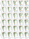 |
Fig. A.1. As in Fig. 2, but for more combinations of αsc and αov. |
| In the text | |
|
Fig. A.2. As in Fig. 2, but now for various αov and initial rotation velocities (indicated in the bottom left of each panel, in units of km s−1). The models were computed with a relatively high time resolution (see Sect. 2) and with αsc = 1. |
| In the text | |
Current usage metrics show cumulative count of Article Views (full-text article views including HTML views, PDF and ePub downloads, according to the available data) and Abstracts Views on Vision4Press platform.
Data correspond to usage on the plateform after 2015. The current usage metrics is available 48-96 hours after online publication and is updated daily on week days.
Initial download of the metrics may take a while.