| Issue |
A&A
Volume 624, April 2019
|
|
|---|---|---|
| Article Number | A97 | |
| Number of page(s) | 14 | |
| Section | Galactic structure, stellar clusters and populations | |
| DOI | https://doi.org/10.1051/0004-6361/201834947 | |
| Published online | 17 April 2019 | |
New bow-shock source with bipolar morphology in the vicinity of Sgr A*
1
I. Physikalisches Institut der Universität zu Köln, Zülpicher Str. 77, 50937 Köln, Germany
e-mail: This email address is being protected from spambots. You need JavaScript enabled to view it.
2
Max-Plank-Institut für Radioastronomie, Auf dem Hügel 69, 53121 Bonn, Germany
3
Center for Theoretical Physics, Polish Academy of Sciences, Al. Lotnikow 32/46, 02-668 Warsaw, Poland
4
Institut für Astro- und Teilchenphysik, Universität Innsbruck, Technikerstr. 25, 6020 Innsbruck, Austria
5
Instituto de Astrofísica de Andalucía – CSIC, Glorieta de Astronomía, s/n, 18008 Granada, Spain
Received:
21
December
2018
Accepted:
13
March
2019
Abstract
Context. We find an extended source in the direct vicinity of Sgr A* with an approximate projected mean distance of 425 ± 26 mas. Its sky-projected elongated shape can be described by an averaged spatial extension of x = 110 ± 20 mas and y = 180 ± 20 mas. With this, the observed object points in the analyzed SINFONI data sets between 2006 and 2016 directly toward the supermassive black hole. We discuss different possible scenarios that could explain the detected blueshifted line emission source.
Aims. Here we present a detailed and extensive analysis of the adaptive optics corrected SINFONI data between 2006 and 2016 with a spatial pixel scale of 0.″025 and a corresponding field of view of 0.″8 × 0.″8 per single data cube with the focus on the newly discovered source. We spectroscopically identify the source, which we name X8, in the blueshifted Brγ line maps. Additionally, an upper limit for the continuum magnitude can be derived from the close-by S-star S41.
Methods. We applied the standard reduction procedure with the SINFONI/EsoRex pipeline for the analysis. We applied pre- and post-data correction in order to establish various calibration procedures. For the sharpened images, we used the Lucy–Richardson algorithm with a low iteration number. For the high-pass filtered images, we used the smooth-subtracting process in order to increase the signal-to-noise ratio.
Results. We are able to detect the elongated line emission source in quantified data sets between 2006 and 2016. We find a lower limit for the infrared continuum magnitude of Ks ≳ 17.0 ± 0.1. The alignment of X8 toward Sgr A* can be detected in data sets that fulfill a sufficient number of observations with a defined quality level. A more detailed analysis of the results shows indications of a bipolar outflow source that might be associated with either a young stellar object, or with a post-AGB star or young planetary nebula.
Conclusions. The near-infrared excess source X8 close to S24, S25, and S41 can be detected between 2006 and 2016. In addition to an apparent bow-shock morphology, the source shows clear signatures of a bipolar outflow that is consistent with both a young stellar object and a post-AGB star. If confirmed, this would be the closest ever detected bipolar outflow source to the supermassive black hole. Similar to the case of the DSO/G2 source and other dusty sources, it further supports the in situ star formation in the direct vicinity of Sgr A*. If X8 were a bow-shock source, it would be the third object of this type that can be found in projection in the mini-cavity. This scenario would support the idea that the cavity is created by a wind from Sgr A*.
Key words: ISM: jets and outflows / black hole physics / protoplanetary disks / Galaxy: center / infrared: galaxies / stars: pre-main sequence
© ESO 2019
1. Introduction
The Galactic center (GC) is a unique laboratory for studying the dynamics of stars and gas in the vicinity of the supermassive black hole (hereafter SMBH) Sgr A*. The nuclear star cluster (NSC) belongs to one of the densest and oldest in the Galaxy, and it therefore contains stars of different ages and masss (see, e.g., Eckart et al. 2005, 2017; Melia 2007; Genzel et al. 2010; Schödel et al. 2014, for reviews). It was argued that the SMBH, hard radiation, shock waves, the considerable magnetic field, and the large velocity dispersion inside molecular clouds makes in situ star formation different from the environment of the Galactic plane (Morris & Serabyn 1996), which directly affects the initial mass function, which is expected to be skewed toward higher stellar masses or have a high low-mass cutoff (Morris 1993; Levin & Beloborodov 2003). The discovery of massive and luminous OB stars within ≲0.5 pc, which were estimated to have formed within the last 10 Myr, led to the formulation of the “paradox of youth” (Ghez et al. 2003). Subsequently, two main scenarios were suggested to account for the presence of young massive stars: a stellar cluster inspiral due to dynamical friction (Gerhard 2001; Kim & Morris 2003), and in situe star formation in a massive gaseous disk (Milosavljević & Loeb 2004); see also Mapelli & Gualandris (2016) for an overview. The cluster inspiral is currently less favored because the inspiral timescales are longer than the estimated age of a few million years of observed OB stars, unless the original cluster contained an intermediate-mass black hole (IMBH; Hansen & Milosavljević 2003), but the contribution of both processes is expected over the whole age of the nuclear star cluster. In particular, the current S-cluster dynamics is consistent with an origin in an initially disk-like stellar cluster around an IMBH that is disrupted close to the SMBH while the IMBH potentially still orbits the SMBH and influences S-cluster dynamics (Merritt et al. 2009). Additional dynamical processes, such as the disruption of binaries close to Sgr A* (Gould & Quillen 2003), may have contributed to the current dynamical state of the NSC.
In addition, the study of the fast-orbiting, early-B type star S2 has given new insights into its spectral properties and its bound elliptical orbit around Sgr A* (see Habibi et al. 2017; Parsa et al. 2017; Gravity Collaboration 2018). Dusty sources with a puzzling near-infrared excess, such as G1 (Witzel et al. 2017) or DSO/G2 (see, e.g., Gillessen et al. 2012; Burkert et al. 2012; Eckart et al. 2013a; Zajaček et al. 2014, 2017a; Witzel et al. 2014; Valencia-S. et al. 2015), provide a unique opportunity to achieve a broader understanding of the circumnuclear medium and its dynamics.
Recently, using high-resolution ALMA observations, Yusef-Zadeh et al. (2017) discovered 11 bipolar-outflow sources in 13CO, H30α, and SiO(5-4) lines that are consistent with having been swept up by jets from young protostars. These outflows exhibit characteristic blue- and redshifted lobes around their central star. Their mass and momentum transfer are consistent with protostellar jets from the Galactic disk population. Bipolar-outflow sources in the GC might manifest a very recent star formation event that took place within 104 − 105 years, which is also supported by the detection of SiO(5-4) clumps and radio-continuum photoevaporative proplyd-like formations within the central parsec (Yusef-Zadeh et al. 2013, 2015). In particular, Yusef-Zadeh et al. (2013) proposed that SiO(5-4) clumps manifest high-mass star formation, while the bipolar-outflow sources analyzed by Yusef-Zadeh et al. (2017) are rather related to low-mass star formation. There is a general consensus that the in situ star formation in the GC region proceeds differently than in the Galactic plane because the massive point source is dominant. This affects the critical Jeans mass through tidal forces. Two main theoretical models of in situ star formation have been developed:
-
Disk-based star formation, when a massive gaseous accretion disk surrounding the SMBH fragments into self-gravitating cores. This occurs when the Toomre stability criterion of a disk Q = csΩ/πGΣ is smaller than unity (Paczynski 1978; Shlosman & Begelman 1987; Levin & Beloborodov 2003; Milosavljević & Loeb 2004; Collin & Zahn 2008).
-
Cloud-based star formation, when an in-falling gaseous clump is prevented from tidal disruption through tidal focusing (Longmore et al. 2013; Jalali et al. 2014), radiation, or wind pressure or by a collision with another cloud, and eventually becomes self-gravitating and fragments into smaller protostellar cores.
Jalali et al. (2014) modeled the cloud-based star formation and showed that it can proceed very close to the SMBH through the gravitational focusing of in-falling cold gas, which can be supplied from the circumnuclear disk (CND). The authors showed that an initially spherical gas cloud becomes tidally stretched as a result of the presence of the SMBH, but at the same time, the cloud becomes compressed in the perpendicular direction. This tidal compression can support the formation of compact young stellar object (YSO) associations similar to the compact comoving IRS13N association of extremely reddened stars (Mužić et al. 2008), which is kinematically distinct from the more evolved IRS13E association members (Maillard et al. 2004). Studying and revealing more potential YSOs near Sgr A* is required to test and improve the current models of in situ star formation in the GC region.
Although many observations of the GC have been carried out by various groups with different telescopes, several unresolved questions remain.
For example, Mužić et al. (2007) discussed a wind or outflow with a magnitude of ∼1000 km s−1 from the direction of Sgr A* that was able to explain the orientation of the comet-shaped sources X7 and X3 toward the central black hole. These bow-shock sources are moving with a proper velocity of around 300 km s−1. Based on the observations carried out by NAOS+CONICA (NACO), which was mounted at the Unit Telescope (UT) 4, the proper motion of X7 is directed toward the north. In comparison, the proper motion of X3 is directed toward the west. Using the SINFONI instrument mounted on the UT4 at the Very Large Telescope (VLT), we are able to partially track source X7 between the epochs 2006 and 2016. It is located southwest of Sgr A* at a distance of 400 mas. We observe a blueshifted line-of-sight (LOS) Brγ velocity of around 645 km s−1 at ∼2.1616 μm and blueshifted lines for HeI at ∼2.0544 μm, Brδ at ∼1.9399 μm, and a weak Paα line at ∼1.8720 μm. The detection in the Brγ line maps shows an elongated emission that matches the position, alignment, and the described shape of the discovered bow-shock source X7 by Mužić et al. (2007).
By applying the same tool set as was used to identify X7 in the SINFONI data set, we investigate a new source that was previously not reported. We call it X8. We find a blueshifted Brγ peak at around 2.164 μm. Additionally, we report a blueshifted HeI line. Weak signs of an H2 line are also detected. However, a confusion with the GC background emission or the overlapping point spread functions (PSFs) of the S-stars S41 and S24/S25 cannot be ruled out. Because of similarities in shape, alignment, and position in X8 and X7, we discuss the possibility of a bow-shock scenario. In addition, the source appears to possess a bipolar morphology and may fall into the mosaic of young stellar sources such as those analyzed by Yusef-Zadeh et al. (2017) in the central parsec. The bipolar outflow could be a manifestation of either a young stellar object or of a late-type star on an asymptotic giant branch (AGB) and at the beginning of a planetary nebular stage.
Hereafter, we explain how the observations were made and describe the data reduction process. After Sect. 2, the analysis Sect. 3 introduces the methods we used, such as high- and low-pass filtering. The results are presented in Sect. 4. Section 5 gives an overview of the different scenarios for the possible nature of X8. We conlude in Sect. 6 and summarize our findings.
2. Observations
2.1. Data sets between 2006 and 2016
We analyzed data between 2006 and 2016 that were downloaded from the ESO archive1 with mainly 600 s for each single data cube. For every year, the final analyzed data cube is a combination of several single data cubes. The total on-source exposure time, which is based on these final data cubes, is listed in Table 1. Additionally, most of the data obtained between 2014 and 2015 were observed with the SINFONI instrument (see Eisenhauer et al. 2003), which is mounted on the VLT/UT4 at Paranal in Chile. As in the downloaded data, we used a H+K (1.45−2.45 μm) grating, but with a 400 s exposure time and a spectral resolution of R ∼ 1500. This translates into a resolving power of 200 km s−1. We used this exposure time setting to be more flexible to accomodate the fast-changing weather conditions. The pixel scale in every analyzed data cube is 12.5 × 25 mas per pixel, that is, the smallest available plate scale. Adaptive optics was enabled. The natural guide star (NGS) we used is located  north and
  east of Sgr A* and has a magnitude of around mag = 14.6. We rejected the use of a laser guide star (LGS) to avoid the cone effect because the blueshifted emission lines of the source might be confused with noise; this is sufficient for the identification to minimize the atmospheric influence. By using an LGS, a decreased data quality cannot be ruled out. The field of view (FOV) was jittered around the position of S2 (see Fig. 1) in a way that the B2V star was located close to the upper right quadrant in the fast-reduction screen. During the observations, the airmass has a direct effect on the data quality. If the acquisition of the starting observations is done with airmass values above 1.6, the AO loop on the NGS is opened and closed during the observations at a airmass of around 1.1–1.2 to increase the performance of the adaptive-optics correction. When we compare the full width at half-maximum (FWHM) of S2 before and after this procedure, we find a quality increase of 10%−20%. The sky that is subtracted in the final reduction procedure is located 5′36″ north and 12′45″ west of Sgr A*. It was observed with an exposure time setting of 400 s in the H+K domain. The science template (o) and the sky template (s) of the SINFONI observation block (OB) was arranged in an o-s-o pattern. This arrangement ensures the highest data quality combined with an efficient observation-time usage. It also minimizes the negative influence on the line shape of weak signals close to the noise level, which is caused by the variation in the sky emission lines (see Davies 2007).
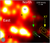 |
Fig. 1. Finding chart of the GC. This is a K-band image of the 2015 observations and is extracted from the associated H+K SINFONI data cube. In the lower left corner, the extracted PSF of S2 of the data cube is shown as a gray elliptical patch. The black cross next to the B2V star S2 marks the position of Sgr A*. North is up, east is to the left. The length of the black bar in the lower left quadrant is |

Properties of X8 between 2006 and 2016.
2.2. Data set of 2005
For the sake of completeness, we recall that data from 2005 are also available in the ESO archive. Unfortunately, this data set does not provide a sufficient number of exposures that cover the area of X8. This leads to a unsatisfying detection of X8, which might also be interpreted as random artifacts. We discuss this briefly below. As described before, the low number of single data cubes, which we stacked to create the final cube, migth cause a shifting centroid position because the on-source time is not long enough to suppress low-frequency peaks caused by the noise. Therefore, the wings of the investigated Brγ line are broader and dominate the emission peak itself. On the other hand, the spectral difference of the line peak between 2005 and 2006 is about 0.000275 μm or ∼38 km s−1. With a resolution in the H+K grating of R = 1640, we calculate a spectral resolution of 0.0013 μm for the peak in 2006. We used K-band data for 2005, with a difference between 2005 and 2006 of 0.00014. The K-band resolution is increased to R = 4490. This results in a spectral resolution of 0.00048 μm. We can therefore conclude that the fluctuations are the result of the limited resolution of SINFONI and the small number of observation nights. It is worth noting that we can also observe these fluctuations over the emission area of X8 by using a single-pixel aperture. Some pixels show a somewhat lower velocity than the majority of the detection. Even though this can be traced back to the scenarios we discussed, it might also indicate the presence of an outflow, a bow-shock feature, or a more complex structure in general.
2.3. Data reduction
We used the standard procedure (ESO pipeline with the GUI Gasgano) to reduce the SINFONI data (see Modigliani et al. 2007). In order to classify the quality of the data, we used the FWHM of S2. The best result can be achieved with an FWHM smaller than 6 pixel in the x- and y-direction for the single data cubes. With a pixel scale of 12.5 mas, this threshold translates into 75 mas in the x- and y-direction. However, values of up to 7.5 pixel (93 mas) for the FWHM can also provide good data quality. This originates in the background emission of the GC and in the overlapping FWHM of the surrounding stars. A case-to-case study is needed to identify data cubes with a sufficient signal-to-noise ratio (S/N). For the instrument setup, dark, linearity, distortion, and wave frames were provided by ESO. After the reduction, we established various data correction procedures. For this, we used DPuser (Eckart & Duhoux 1991, and T. Ott) and IDL routines. First, we removed bad pixels that were located mostly at the border of the data cubes. This is important for the stacking of the individual cubes that takes place at the end of the correction process. The result would be reflected in non-continuous pixel values. Second, we corrected for the pixel-to-pixel variations on the detector by multiplying single rows with a proper factor. After this, the telluric absorption was corrected by taking several aperture star spectra from data cubes that were combined by individual days. The IDL routine applied a polynomial fit to every spectra and corrected the telluric absorption afterward. In the last step, we stacked the already shifted and normalized data cubes according to a reference frame that was created with single K-band images of the GC. The K-band images were extracted from single SINFONI data cubes by selecting the wavelength range between 2.0 μm–2.2 μm. By choosing sufficient cubes, a continuum reference frame with  was created.
3. Analysis
For the analysis we used different techniques that we introduce in the following subsections. We describe tools like high-pass and low-pass filtering. Followed by that, we explain the extraction process for line and continuum maps.
3.1. High-pass filtering
Overlapping PSFs and noise can complicate the identification of the X8 source, therefore we used high-pass filtering to decrease the chance of confusion and to identify single objects that were close to the detection limit. Not only can the quality of the data influence the detection of X8, but the close distance to S24, S25, and S41 also plays a major role in the analysis of the source. Figure 2 shows the blueshifted Brγ line map (right subplot). The figure shows that X8 is partially blocked by the S star S41. Therefore, high-pass filtering cannot be used to identify X8 in the continuum. However, it can be used to determine a upper limit for the magnitude. The PSF of this star decreases the chance of a successful identification in the continuum. For the smooth-subtracted image (middle subplot), we used the filtering technique that is described in Mužić et al. (2007). The authors subtracted a Gaussian-smoothed version of the original continuum image and smoothed the output again. With this, high frequencies pass, while low frequencies, such as noise, are reduced. Because of different weather conditions and consequently different PSFs between 2006 and 2016, we adjusted the Gaussian to 3–5 pixels for the subtracted and re-smoothed continuum images.
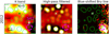 |
Fig. 2. Galactic center in 2012 observed with SINFONI with a DIT of 600 s for each single data cube. In total, 61 data cubes are combined with an integrated exposure time of 610 min. The resulting on-source exposure time of the final data cube is around 10 h. North is up, east is to the left. The lime contour lines are based on the middle high-pass filtered image. It shows matching positions for the stars in the left K-band image. It is extracted from the SINFONI H+K data cube. The cross marks the position of Sgr A*. The magenta dashed circle indicates the position of S41. This S-star is in superposition with X8, which is displayed in the right image (bright white object in the lower right corner). This subplot is a blueshifted line map with respect to the Brγ rest wavelength at 2.1661 μm. |
3.2. Low-pass filtering
The crowded FOV in the GC demands additional filtering techniques. The iterative Lucy–Richardson deconvolution algorithm (Lucy 1974) can be used to sharpen the image. For this, we used 20 iterations and analyzed the convolved image without deconvolving the result. The small number of iterations preserved the positions of the stars in the field of view and ensured that no artificial sources were created. Therefore, analyzing the convolved image is justified. We extracted a K-band image from the final data cube by selecting the spectral range between 2.0 μm–2.2 μm. Because the final data cube is a stacked result of many single observations that are observed under different weather conditions, an artificially created PSF can reflect this circumstance with satisfying results. The only star that can be used to extract a natural PSF in the GC with SINFONI in an FOV of  around Sgr A* is S2. However, some stars, such as S13, S56, and S64, are in superposition with S2. Therefore, a natural PSF will not lead to representative results for the GC region. An artificial PSF (APSF) neglects the influence of overlapping PSFs. It can be created by applying a Gaussian filter to an empty array. The size needs to match the dimensions of the analyzed data. For the extracted K-band image, we used an APSF that was rotated by 45° (counterclockwise) with a spatial extension of 4.0 pixel in x- and 4.5 pixel in y-direction. The size of the K-band image and the APSF array was increased to 256 × 256 pixel. S2 is centered at (128, 128), and the same centering was applied to the APSF. After the setup of the normalized files, the Lucy–Richardson algorithm (QFitsView, T. Ott) was used to sharpen the image.
3.3. Line and continuum maps
The line maps represent the blueshifted Brγ emission at 2.164 μm. Compared to the blueshifted Brγ line, the HeI emission line is characterized by a decreased intensity of ∼50%. The more prominent blueshifted Paα line shows an increased level of confusion due to the telluric absorption lines. This line is therefore excluded and is not discussed in the further analysis. The Brγ line maps were achieved by subtracting the K-band continuum from the emission peak itself. In addition, we stacked Brγ line maps of several years that fulfilled the requirements for the FOV and data quality. This was done by shifting the individual line maps of X8 to a fixed position. We used the center of gravity of the 50% contour line to determine the exact position of X8. The white inset located in the upper left quadrant in the image shows a cut along the alignment axis, which is directed toward Sgr A*. For the high-pass filtered image (Fig. 2, middle), a continuum frame from the final combined data cube was used. We selected the spectral range of 2.0 μm–2.2 μm in the SINFONI data cube and extracted the K-band continuum image. After this, the image was normalized.
4. Results
In this section we apply the methods and tools of Sect. 3 to the discovered X8 source. With these tools, we were also able to detect the confirmed bow-shock source X7 in selected data sets.
4.1. X7 detection
Based on the analyzing tools presented in Sect. 3, we identified the bow-shock source X7 (see Mužić et al. 2007, 2010) in the available SINFONI data set between 2006 and 2016. The investigated line maps of the data cubes show a blueshifted Brγ line at ∼2.1614 μm with a related velocity of about 645 km s−1. The contour of the X7 line map is shown in Fig. 1. The spectral analysis also shows blueshifted lines for HeI at ∼2.0544 μm (∼625 km s−1), Brδ at ∼1.9399 μm (∼800 km s−1), and a Paα μm line at ∼1.8720 μm ( ∼ 577 km s−1). We also detected a CO line at 2.3226 μm in the spectrum of X7. However, the line-map analysis does not show an emission counterpart. Because this wavelength corresponds to the CO rest wavelength, we can conclude that this line likely belongs to the background or foreground emission.
With a spectral uncertainty of around 100 km s−1 and the non-negligible influence of telluric absorption lines, the additional velocities are in agreement with the detected blueshifted Brγ line speed. The K-band continuum is dominated by background emission and stars that are close to X7. Especially S32 (see Fig. 3) is in superposition with the K-band continuum emission of X7 and contributes to the confusion of detecting the bow-shock source. Mužić et al. (2010) derived a K-band magnitude for X7 of mag = 16.9 ± 0.1. For the K-band magnitude of star S32, Gillessen et al. (2009) derived a magnitude of mag = 16.6. With the reference star S2, we calculate a magnitude for S32 of mag = 17.06 ± 0.06 based on the data cube of 2013. This results in an averaged magnitude of mag = 16.83 ± 0.06. These mixed results are reflected by the circumstance that X7 and S32 coincide in position and magnitude. However, this leads to unsatisfactory results when the smooth-subtract algorithm is used to identify X7 in our K-band continuum data. With respect to X7, X8 exhibits comparable properties (position, magnitude, composition, alignment, and LOS velocity). In this picture, X7 and X8 are likely of the same nature and might be of the same origin. Hence, X8 seems to be the third observed bow-shock source that can be found in projection in the mini-cavity, which is assumed to be created by a wind or outflow emanating from the direction of Sgr A*.
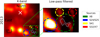 |
Fig. 3. Galactic center in 2013. The on-source observation time is almost 30 h. Here we extracted a K-band image from the final data cube. On the right side, a zoomed-in and low-pass filtered image of the green rectangle area is presented. The green dashed circle shows the position of X8. The contour line is based on the blueshifted Brγ line map of 2013. |
4.2. X8 detection
In Fig. 4 we present a selection of the X8 detection in the SINFONI data covering three years (2006, 2012, and 2015). The first column shows a blueshifted Brγ line map with continuum contours that are extracted from the final data cubes. The position of Sgr A* is marked with a white cross. We centered every line map on the position of Sgr A* at (44, 47) in the 100 × 100 pixel array. The B2V star S2 is indicated by its name, while a white arrow (fixed position in every presented line map) shows the source X8. Based on the derived position of Sgr A*, X8 moves with a proper motion of around 300 km s−1 away from the SMBH. X8 can be found in every year in a comparable area. It is slightly elongated, with a mean FWHM of x = 110 mas and y = 180 mas. This indicates an extended shape because the SINFONI PSF is about 60–80 mas in x- and y-direction. In the data set we present here, we also detect hints of the D2 and D3 dust sources (Eckart et al. 2013b) at the upper right border of the FOV. The second column of Fig. 4 shows the related spectroscopic K-band emission lines of X8 that are extracted with a five-pixel circular aperture from the final data cubes. We find blueshifted lines such as Brγ at 2.164 μm and HeI at 2.057 μm with an FWHM of about 170 km s−1. These wavelengths correspond to an averaged blueshifted velocity of ∼200 km s−1 with respect to their corresponding rest wavelengths at 2.1661 μm (Brγ) and 2.0586 μm (HeI). Additionally, we find two other lines at 2.2176 μm and 2.3471 μm. It is not clear to which rest wavelength these lines can be linked beause either the resulting velocity does not match the blueshifted Brγ and HeI lines or the lines match the velocity, but are redshifted instead. These emission lines are weaker than the detected Brγ and HeI by a factor of 2–4 and are not free of confusion. The background and surrounding stars mainly influence the detection of X8. The data quality, the amount of data, and the weather conditions also play a non-negligible role in the analysis of X8, however. It might be speculated that these lines indicate a more complex structure or possible outflow properties. For Fig. 5 we used the individual blueshifted Brγ line maps. We selected data cubes that matched our requirements in terms of the field of view and data quality. Then we applied a shifting vector to the line maps such that X8 was at the same position in every data set. At the expected position of X8, the stacked result shows an elongated object that points toward Sgr A*. It shows two central lobes that are highlighted with blue contour lines at 60% and 90%. The white inset is a 2D cut along the alignment of X8 and reflects the finding of the two emission peaks, which are about 12.5–25 mas apart. The two lobes are embedded in the elongated and blueshifted Brγ source. The object itself is directed toward Sgr A*, which is represented here with a green cross for every single year. Because Fig. 5 is a stacked image of several years of a moving source, Sgr A* seems to move. Of course, sourche X8 moves, and the shift of Sgr A* reflects its motion because the reference frame is centered on it. The Brγ emission sources D2 and D3 can be partially found at the right border in the upper FOV because the blueshifted wavelength of the two sources is close to the X8 emission. Another faint emission source is also visible around  in the y-direction above Sgr A*.
4.3. Proper motion and line-of-sight velocity
To determine the proper motion, we inferred the offset between X8 and Sgr A* in the blueshifted Brγ line map in 2006 (386 mas) and 2015 (462 mas). In order to pinpoint the exact distance, we used the center of gravity of the 50% contour line in the channel maps. These measurements resulted in Δd = 70 mas for X8 between 2006 and 2015. With a distance to the GC of 8 kpc and the time difference between 2006 and 2015, we obtain a proper motion of v = 293 ± 20 km s−1. For the LOS velocity (Fig. 6), we used the blueshifted HeI and Brγ centroid line. The blueshifted HeI line and the blueshifted Brγ line detection are free of confusion because they were spectrally isolated. However, we derive a mean HeI velocity of v = 210 ± 20 km s−1, whereas the slightly increased Brγ velocity is v = 220 ± 20km s−1. These variations between the blueshifted HeI and Brγ line detection are based on the spectral resolution and instrumental effects that are described in Eisenhauer et al. (2003). It shows that the LOS velocity is constant within uncertainties for all epochs. This is also reflected in the spectrum of X8 (see Fig. 4). The average velocity is about 215 km s−1 and therefore close to the detected proper motion of about v = 290 km s−1.
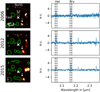 |
Fig. 4. Blueshifted Brγ line maps of the GC at 2.164 μm (left) that are based on the data sets of 2006, 2012, and 2015. The green contour lines are extracted from the K-band continuum emission of the associated data cubes. Sgr A* is located at the cross, the S star S2 is labeled. The arrow points toward the position of X8 in the blueshifted Brγ line maps in 2006, 2012, and 2015. The cross is centered on SgrA* in every year. The arrow is fixed on the position of X8 in 2006 to show the proper motion. On the right side, the K-band spectrum between 2.0 μm–2.4 μm of X8 is presented. The intensity is given in arbitrary units (a.u.), and the blueshifted HeI and Brγ line are framed with a dashed line. The spectrum of 2012 and 2015 shows the blueshifted [Fe III] multiplet 3G − 3H at 2.1410 μm, 2.2142 μm, 2.2379 μm, and 2.3436 μm. |
4.4. Velocity gradient
As indicated in Fig. 5, the blueshifted source X8 contains two central lobes. With a constant FWHM of about 170 km s−1, we were able to select the red and blue wing of the Brγ emission line. The blueshifted wing is faster than the Brγ rest wavelength and covers the wavelength range between 2.16394 μm–2.16455 μm. The slower redshifted wing of the emission line covers a range of 2.16455 μm–2.16516 μm. With this, we detect a velocity gradient over X8 that is reflected by a variation of the emission toward a certain area of the blueshifted Brγ source as a function of the selected wavelength range. The mean velocity of the velocity gradient slope is about 215 km s−1. The mean velocity of the blueshifted wing is 177 ± 38 km s−1, whereas the mean velocity of the redshifted wing is 257 ± 42 km s−1. With this, the velocity gradient can be determined to be 45 ± 10 km s−1/12.5 mas.
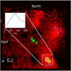 |
Fig. 5. Stacked Brγ line map showing X8. The image is based on the 2006, 2012, 2013, 2015, and 2016 data sets. The data sets of 2008, 2009, 2010, 2011, and 2014 partially cover the X8 emission area or show effects from a reduced S/N. Because non-continuous effects can be found at the border of the data cube, the data sets of 2008, 2009, 2010, 2011, and 2014 were excluded from the stacking. The low S/N reflects that only a few exposures cover the X8 emission area or that the data-cube correction was unsatisfactory. Because the single Brγ line maps of 2006, 2012, 2013, 2015, and 2016 are centered on X8, the stacked figure implies an apparent movement of Sgr A*, which is indicated by a green cross. The y-axis of the white patch in the upper left corner is in arbitrary units (a.u.). |
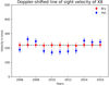 |
Fig. 6. Line-of-sight of X8 between 2006 and 2016. It is based on the blueshifted centroid Brγ (red data points) and HeI (blue data points) velocity of X8 with an error of ±20 km s−1 for every data point. The dashed line represents a linear fit to the blueshifted Brγ data points. |
Figure 7 shows the line maps we obtain when we select the red and blue wing of the emission line. The resulting line map that is achieved by selecting the 2.16455 μm–2.16516 μm wavelength range is associated with the red lobe. It is slower than the blue lobe with respect to the Brγ rest wavelength at 2.1661 μm. The corresponding blue lobe is obtained by selecting the 2.16394 μm–2.16455 μm wavelength range. However, when we select the whole Brγ emission peak with a central wavelength of about 2.16455 μm, both lobes are visible in the line maps that are presented in Fig. 7. This excludes the possibility that the lobes just represent the velocity of the source itself because the two emission peaks can be detected individually in 2006 and 2012. It should be noted that the distance between the faster blue lobe and Sgr A* is about 380 ± 13 mas. For the slower red lobe, the distance is 420 ± 13 mas. Hence, the faster blue lobe is closer to the SMBH than the slower red lobe.
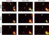 |
Fig. 7. Blueshifted Brγ line maps of X8 in 2006 and 2012. A scale valid for all images is given in the top left panel. The last row shows the stacked result of 2006 and 2012 with an averaged position of Sgr A* (white cross) that is based on the years we present. The red lobe column represents the wavelength range of 2.16455 μm–2.16516 μm. The blue lobe results cover a wavelength range of 2.16394 μm–2.16455 μm. For the last column, we select the wavelength range of 2.16394 μm–2.16516 μm so that both lobes are visible. |
4.5. Continuum emission
Because of the close distance of S41 (see Fig. 2), we are only able to provide an upper limit on the flux and brightness of X8. The spectroscopic data of the emission area of X8 show a weak H2 line that can be associated with the S star. This is followed by the conclusion that X8 has to be fainter than S41. Figure 2 shows the S star S41 in 2012; it is located inside the magenta dashed circle. Figure 3 shows the same situation, but in 2013, where in contrast to the former image, X8 and S41 are separated. This shows that the PSF and therefore the data quality influences the detection of X8. Sgr A* in Figs. 2 and 3 is located at the cross (black and white). The contour lines in Fig. 2 (left and right) are taken from the middle figure, where we present a high-pass filtered version of the left K-band image. It shows the positional robustness of the high-pass filtering technique. A three-pixel Gaussian was used to smooth the K-band image. After this, the smoothed output image was subtracted from the K-band image. The resulting smooth-subtracted image was again smoothed with a three-pixel Gaussian. The final image shows the faint star S41 roughly at the position of X8. For a better comparison, a combination of the blueshifted Brγ line map of X8 and the continuum contour lines from the high-pass filtered image is shown in the right figure. For S41, we derive a magnitude of mag = 16.91 ± 0.06 with a flux of (0.107 ± 0.006) × 10−3 Jy. The error is based on the literature values for the calibration star S2 (see Schödel et al. 2009). In principal, the error should just cover the range between mag = 16.91 + 0.06 because lower values would result in a brighter star. Considering that this S star is not detected between 2006-2016, the K-band magnitude is most reasonable at the end of the range. If X8 is as bright as S41, we would be able to detect an even brighter and elongated source because the flux would add up. From this, we can derive a lower K-band magnitude limit of mag = 16.97 with a flux of (0.107 ± 0.006) × 10−3 Jy for X8. In Fig. 3 we investigate the GC with a low-pass filter. The zoomed area shows the S stars S24, S25, and S41. X8 can be detected at the position of the blueshifted Brγ line map. Remnants of X7 can also be detected, although the chance of confusion with S32 cannot be ruled out. The 90% level contour lines of X8 are based on the blueshifted Brγ line map of 2013. Because the zoomed and low-pass filtered image is not convolved with a PSF because of the low iteration number, we are able to detect X8. We therefore conclude that the detected emission is produced by gas and dust.
4.6. [Fe III] line
In addition to the presented KS-band spectrum, we report a simultaneously detected blueshifted [Fe III] line for X7 as well as for X8. We identify the ionized blueshifted [Fe III] multiplet 3G − 3H for X7 and X8 in our data set in 2015. Because of the limited FOV and the dynamic data quality, we gave greater weight to the data set of 2015 in our comparison of X7 and X8. The velocities, wavelengths, and the transition state of these lines are listed in Table 2. The mean velocity of the blueshifted [Fe III] multiplet is slightly decreased compared to the mean velocity between the blueshifted Brγ and HeI line for both sources. The line maps for X7 and X8 are based on the blueshifted [Fe III] lines and are in spatial agreement with the Brγ and HeI analyses. These line maps and the related spectrum are shown in Figs. 8 and 9. While the blueshifted [Fe III] X8 detection is in agreement with the HeI and Brγ emission, the X7 [Fe III] multiplet is dominated by the continuum for the 3G3 − 3H4 and 3G4 − 3H4 lines. In contrast, the 3G5 − 3H6 and 3G5 − 3H5 lines coincide spatially with the blueshifted HeI and Brγ channel maps.
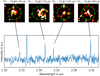 |
Fig. 8. Blueshifted [Fe III] line maps of X8 in 2015. The spectrum shows the [Fe III] multiplet. At 2.164 μm, the prominent blueshifted Brγ is located. The four line maps are a 19 × 19 px (230 × 230 mas) cutout from the data cube of 2015. |
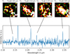 |
Fig. 9. Spectrum of X7 in 2015. It shows the blueshifted [Fe III] multiplet and the related 19 × 19 px (230 × 230 mas) line-map cutouts. The prominent blueshifted Brγ can be found at 2.161 μm. |
Detected blueshifted [Fe III] line velocities of X7 and X8 in 2015.
5. Discussion
In this section, we discuss several possible scenarios concerning the nature of X8. We also provide orbital constraints and the location of the source inside the NSC.
5.1. X8 detection and the optical depth
Based on the detection presented in Fig. 3, we can confirm a continuum counterpart to the blueshifted line detection of X8. The detected source in the continuum shows a similar elongated shape as its gaseous counterpart. The elongation is underlined by the x- and y-expansion measurements presented in Table 1. In both directions, the dimension of X8 exceeds the SINFONI PSF. Therefore, the observed source emission is extended and not compact. We detect two separate main emission peaks. These two peaks can be each linked to the detected lobes. This could indicate a more complex structure. Because the faster lobe is located closer to Sgr A* than the slower lobe, it can be speculated that the presence of a possible wind from Sgr A* or a wind of the source itself causes this setup. Because the proper motion is directed away from the SMBH, this asymmetrical system could be influenced by either external or internal winds. Another possibility could be an outflow from massive stars around Sgr A*. Mužić et al. (2007) concluded that a wind from massive stars around Sgr A* is a less plausible scenario. The  ratio for the optical depth is ∼0.7. This indicates optically thin material (see also Shcherbakov 2014). Even though the continuum detection could be partially dominated by the blueshifted line emission, the continuum counterpart of X8 can be assumed to be optically thick stellar or dust photosphere. To distinguish between potential stellar and dust contributions to the continuum, further observations in L′ and M bands are needed.
5.2. Closest bipolar outflow source to Sgr A*
As shown by Yusef-Zadeh et al. (2017), 11 bipolar outflow sources are close to Sgr A* and are located within a projected distance of 1 pc from the SMBH. The authors report sources that show similarities to the detected features of X8. The detected source BP1 (Yusef-Zadeh et al. 2017) is described as two bright lobes that are embedded in a molecular cloud. This scenario could explain the detection of X8 that we present in Fig. 5. The detection of GL2591 (see Tamura & Yamashita 1992 for more details) also shows a similar 2D cut as we find for X8 (Fig. 5). To verify the detection of the two-lobe feature, we also show Brγ line maps, where we only selected the red- and blueshifted wing of the Doppler-shifted Brγ emission peak. As shown in Fig. 7, the detection of the two lobes depends on which wing of the Brγ emission peak is selected. This can be translated into the identification of a blue- and redshifted lobe for X8, whereas the blue lobe is closer to Sgr A*. This means that the red lobe is farther away from the supermassive black hole. The quality of the data is not stable because the weather conditions varied, therefore we present two examples and a stacked version of the two data sets. Even though noise and background features in the presented data increase the level of confusion for the detection of X8, the results presented in Fig. 7 clearly support a two-lobe scenario.
5.3. X8: a possible bow-shock source
In addition to exhibiting a bipolar morphology, the outflow associated with X8 is also likely to drive a shock into the surrounding medium because most stars in the inner parsec are expected to move close to the local sound speed (see Zajaček et al. 2017b, especially their Fig. 1). The Brγ emission of X8 traces ionized gas and appears to be directed toward Sgr A*. The position angle between Sgr A* and X8 is about 45° in 2006 and 55° in 2016. Because we detect a proper motion of X8, the change in angle can be explained by its trajectory. Especially in Fig. 1, which is based on the data set in 2015, shows similarities between the bow-shock source X7 and X8. However, we also observe the influence on the data that is caused by the background and overall quality (see Figs. 2 and 3). It is therefore a reasonable possibility that the two-lobe structure of X8 in 2015 cannot be detected because of the influence we described above. Under the assumption that X8 drives a bow shock into the ambient medium, the bipolar outflow of X8 could be influenced by a potential external wind from the direction of Sgr A* (see Mužić et al. 2010). It would be the third bow-shock source that (at least in projection) lies in the mini-cavity, which is assumed to be generated by the outflow. The detected blueshifted [Fe III] line might also be an indicator for wind that spatially originates at the position of SgrA* because the ionization of iron needs high energies (around 35 000 K, see Likkel et al. (2006) for further information). The line ratio between [Fe III] and Brγ for planetary nebulas (PNs), which is found in Likkel et al. (2006), is about 2%. However, the line ratio between [Fe III] and Brγ for X8 is about 45%. Therefore, we can exclude the intrinsic scenario, and the external origin for [Fe III], in particular a bow shock, are more likely. In other words, if the excitation cannot be explained completely by intrinsic processes, an external wind that has been inferred from the detected X3 and X7 sources (Mužić et al. 2010) can explain this high line ratio. In addition, an outflow also determines the overall bow-shock orientation if the outflow velocity is higher than the stellar velocity because the bow shock is oriented along the relative velocity, vrel = v⋆ − vambient (see also the discussion in Mužić et al. 2010; Zajaček et al. 2016). The fact that we find comparable [Fe III] to Brγ ratios for X7 of about 40% could point to a similar nature of X8 and X7.
5.4. Orbital constraints, location within the NSC, and basic hydrodynamics of X8
Source X8, with its mean projected distance R ∼ 425 ± 26 mas = 0.017 ± 0.001 pc, appears to lie in the innermost parts of the NSC in either the clock-wise disk or the S cluster, which are inside ∼0.4 pc. If this is confirmed, the presence of either a protostar or an AGB star would have implications for their origin and dynamics because it was previously assumed that S-cluster members are rather B-type stars or dwarfs (spectral type in the range of B0-B3V) with an upper age limit of 15 Myr (Habibi et al. 2017) and that the clock-wise disk stars are of spectral type OB, with a similar age constraint of a few million years (Bartko et al. 2010).
Because X8 is well inside the gravitational influence of Sgr A*, which is estimated for the GC to be rh ≈ 2 pc, we can assume that it is bound and orbits Sgr A* on an elliptical orbit as other S stars do. Its radial velocity of vr = 215 km s−1 is blueshifted, whereas the tangential component vt = (293 ± 20) km s−1 points away from Sgr A*. The total space velocity of the star then is  . Because the radial and the tangential velocity components are of a comparable magnitude, we can assume that the X8 orbit is close to edge-on with the current X8 position in the background with respect to Sgr A* and moving toward us, see Fig. 10 for an illustration. We can also infer the position along the orbit: the true anomaly ϕ = 90 ° +ϕ0 from the decomposition of the velocity vector, tanϕ0 = vt/vr, from which ϕ = 90 ° +53.7 ° =143.7°.
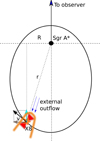 |
Fig. 10. Illustration of the eccentric X8 and its current position in the background with respect to Sgr A*. The bipolar morphology and the bow-shock orientation are also depicted. |
The orbit is not consistent with zero eccentricity. If the orbit were circular, we could estimate the 3D distance from Sgr A* simply as  . From Fig. 10, the orbital phase then would be ϕ′ = 172.8°, which disagrees with the velocity-based calculation. Instead, we can look for a series of orbital solutions (a, e) with a non-zero eccentricity e and semi-major axis a given the true anomaly of ϕ = 143.7° and the total velocity v⋆ = 363.4 km s−1. An exemplary calculation can be made for the mean eccentricity
  of the thermal distribution of eccentricities n(e)de = 2ede, which appears to be a good approximation for the S stars (Genzel et al. 2010). By combining the velocity and radius equations for the elliptical orbit, we obtain a semi-major axis of X8, aX8 = 0.09 pc. The position of X8 with respect to the observer is illustrated in Fig. 10 for a moderately eccentric orbit.
The semi-major axis of X8 as a function of eccentricity in the range (0, 1) is plotted in Fig. 11. The semi-major axis is on the order of aX8 ≈ 0.1 pc because eccentricity values higher than 0.9 are unlikely. X8 therefore falls into the same range of semi-major axes as the young massive stars in the clock-wise disk and the scattered population (Genzel et al. 2010). Although corrections to these estimates are necessary with a proper orbital analysis with more data, we have at least shown that source X8 is fully consistent with being located inside the NSC in its inner parts.
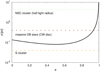 |
Fig. 11. Calculated semi-major axis of the X8 source as a function of its eccentricity assuming an edge-on elliptical orbit. The horizontal lines mark the characteristic scales of the known young stellar populations in the GC region: S stars and CW disk members (Genzel et al. 2010). The uppermost line marks the half-light radius of the NSC, rhl = (4.2 ± 0.4) pc, according to Schödel et al. (2014). |
Source X8 moves away from Sgr A*, but the symmetry axis of the extended Brγ emission points toward Sgr A*. This can be explained by the bow-shock formation when the orbiting X8 interacts with an outflow of vout ≈ 1000 km s−1 from the direction of Sgr A*, in a similar way as for the comet-shaped sources X3 and X7 (Mužić et al. 2010). The characteristic size of the bow shock is given by the stagnation radius (Zhang & Zheng 1997),
 (1)
(1)
at which the stellar wind pressure and the ram pressure are at equilibrium. In Eq. (1) ṁw and vw are the stellar mass-loss rate and the terminal wind velocity, respectively, and Ω is the solid angle into which the stellar wind is blown. ρa denotes the ambient density, and vrel is the relative velocity of X8 with respect to the outflowing ambient medium. The solid angle is given by Ω = 2π(1 − cosθ0), where θ0 is the opening angle of the outflow.
For X8 we can estimate several parameters in Eq. (1). The stagnation radius of X8 is about R0 ∼ 100 mas ∼ 825 AU, as indicated by the intensity profile in Fig. 5. The terminal wind velocity can be estimated based on the FWHM of Brγ line, vw ∼ 170 km s−1. The opening angle of the bipolar outflow can again be approximated by θ0 ∼ 45° from the brightness distribution in Fig. 5. The relative velocity vector is given by the vector difference between the stellar motion and ambient medium flow. With the approximation that the external outflow is directed perpendicular to the orbital velocity, the relative velocity magnitude can be estimated as  . Finally, the ambient density at the estimated deprojected distance of X8, rX8 ∼ 0.1 pc, can be calculated from the ADAF profile of Xu et al. (2006), na ∼ 104(r/1015 cm)−1 cm−3, with the mass density ρa ≈ mHna. Subsequently, this allows us to search for the mass-loss rate of X8 that is consistent with the observed bow-shock size of R0. In Fig. 12 we plot the stagnation radius R0 as a function of the mass-loss rate. The observed stagnation-point size of 100 mas is consistent with the mass-loss rate of X8 of ṁw = 10−6.8 M⊙ yr−1, which is a realistic value for both protostars and post-AGB stars, as we discuss further in the following subsection.
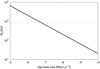 |
Fig. 12. Stagnation radius of a stellar bow shock as a function of its mass-loss rate according to Eq. (1). The other parameters were fixed based on observed values, as discussed in the text. The horizontal line marks the stagnation radius as estimated from the brightness profile in Fig. 5. |
5.5. Plausible scenarios for the origin of X8
The elongated, bipolar geometry of X8 is consistent with two scenarios that we discuss below.
– Dust-embedded YSO. In general, young stellar objects are naturally characterized by axisymmetric geometry caused by their rotationally flattened dusty envelopes (Ulrich 1976). Depending on the YSO stage (stage 0, I, II, or III according to Lada 1987), the envelope becomes progressively geometrically thinner and the accretion rate onto the star becomes slows down. The X8 source would be consistent with an YSO stage of class I surrounded by optically thick dusty envelope dissected by bipolar outflows. This scenario was also envisaged for the unresolved dusty S-cluster object (DSO/G2), see Shahzamanian et al. (2016) and Zajaček et al. (2017a) for detailed radiative transfer simulations. In a similar way, the massive young stellar object NGC 3603 IRS 9A* shows clear signs of a disk–bipolar cavity (Sanchez-Bermudez et al. 2016). The Brγ lobes could be associated with ionized outflows in the cavities. The bipolar outflow is expected to further interact with the ionized wind from the direction of Sgr A* (Mužić et al. 2010; Sabha et al. 2014) with an estimated terminal velocity of ∼1000 km s−1, which is expected to result in a bow shock that is driven into the ambient medium (Scoville & Burkert 2013). This shock would be rather diluted, but could contribute to the overall elongation of X8 along the Sgr A*–X8 connection line. The dusty envelope would be oriented perpendicular to the outflow; see the illustration in Fig. 13 for a geometrical illustration of X8 as an YSO source.
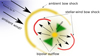 |
Fig. 13. Illustration of the possible interpretation of X8 as a bipolar young stellar object of class I. We show the approximately |

– Post-AGB star or young planetary nebula. In addition to young stellar objects, bipolar outflows are associated with the final stages of stellar evolution, that is, with collimated winds from red giants and post-AGB stars in the early planetary nebula phase (Frank 1999). The bipolarity could be formed during the early planetary nebula stage, when the detached gas from aging stars is collimated by a magnetic field or by a companion star (Kwok 2000; Chen et al. 2017). Bipolar planetary nebulae resemble young stellar objects in many ways, such as emission that traces ionized gas with similar line widths.
Without further spectroscopic evidence, we cannot clearly clasify X8 as either a YSO or a post-AGB star. Statistically, given the presence of other young stars in the region, including proplyd, bipolar, and dusty sources (Eckart et al. 2013b; Yusef-Zadeh et al. 2015, 2017), we can hypothesize that X8 is another manifestation of a recent star formation event. However, the YSO and young planetary nebula scenario both imply that X8 belongs to the extreme populations of the nuclear star cluster, that is, to either very young or old stars and out of the main sequence. A more detailed analysis of this and similar sources can complement previous population synthesis studies (Buchholz et al. 2009; Gallego-Cano et al. 2018) and thus shed more light on the rich episodic star formation history of the nuclear star cluster (Pfuhl et al. 2011).
Based on the observational properties of X8 and its stability over the years, we consider the following scenarios. They might in theory resemble a bow shock and bipolar morphology.
– Supernova. Massive stars in the central parsec of the GC will end their lives as supernovae with an approximate rate of ṄSN ≈ 10−4 yr−1. The supernova explosions are not symmetric, which results in initial neutron stars and black hole velocity kicks. The initial expansion velocities of the supernova shell are, however, one order higher than what we measure for the Brγ line, on the order of ∼1000 km s−1. Moreover, supernova explosions would manifest themselves by nonthermal radio emission and high-energy radiation in X-rays and γ-rays. Because no such event has been detected recently, we consider the supernova origin of X8 unlikely.
– Core-less cloud. The overall stability and bipolar nature of the source are inconsistent with a gaseous-dusty cloud without any stellar core. Any core-less cloud would have a tendency to become dispersed in a highly ionizing medium and/or become more elongated or filamentary through interaction with the nuclear outflow. This is underlined by theblueshifted [Fe III] multiplet 3G − 3H that we reported here.
6. Conclusion
We provided an overview of possible scenarios for the object X8. We observed X8 in every year in the blueshifted emission line maps in combination with the K-band continuum detection. Our observations indicate a star-like scenario with a possible bow shock. The detected two lobes moreover show different velocities. The lobe closer to Sgr A* is faster than the lobe that is farther away. This could be explained with intrinsic properties. External effects that cause this velocity gradient cannot be ruled out either. Because this setup of two different lobes with different velocities can be observed over a time-span of almost 15 years, a central star that stabilizes this system is a reasonable explanation. In contrast, a pure gas-cloud identity close to S stars S24, S25, and S41 would result in dissolving scenarios. Moreover, gas would probably not be arranged in a complex structure with two individual detectable lobes that show different velocities. The detected blueshifted [Fe III] can be associated with high temperatures that also rule out a purely gaseous nature of X8. If future observations can reveal the stellar component of X8, the source would indeed be one of the closest YSO to Sgr A* to date. Because X8 is moving away from S24 and S25, the object becomes more isolated. A more detailed analysis that is covered by near-infrared observations could provide more properties of the two lobes. These findings could then confirm the closest bipolar outflow source to Sgr A*. Even today, howevr, we observe strong evidence that supports this possibility. The two individual lobes can be observed in our high-quality stacked images and in the data cubes of different years. The limiting factor in every case is the quality and number of observations that cover the western region next to S24 and S25. Nevertheless, this indicates that the two-lobe feature is not a stacking feature. The individual lobes, which are shown in the line maps, were extracted by selecting the blue and red lobe of the blueshifted Brγ peak (with respect to the rest wavelength) and therefore support the idea that these are two individual lobes with two velocities.
Acknowledgments
We highly appreciate the comments of the anonymous referee that helped to improve this paper. We received funding from the European Union Seventh Framework Program (FP7/2013-2017) under grant agreement no 312789 – Strong gravity: Probing Strong Gravity by Black Holes Across the Range of Masses. Michal Zajaček acknowledges the support by the National Science Centre, Poland, grant No. 2017/26/A/ST9/00756 (Maestro 9). This work was supported in part by the Deutsche Forschungsgemeinschaft (DFG) via the Cologne Bonn Graduate School (BCGS), the Max Planck Society through the International Max Planck Research School (IMPRS) for Astronomy and Astrophysics, as well as special funds through the University of Cologne and SFB 956 – Conditions and Impact of Star Formation. Part of this work was supported by fruitful discussions with members of the European Union funded COST Action MP0905: Black Holes in a Violent Universe and the Czech Science Foundation – DFG collaboration (No. 13-00070J). We also would like to thank the members of the SINFONI and ESO Paranal/Chile team.
References
- Bartko, H., Martins, F., Trippe, S., et al. 2010, ApJ, 708, 834 [NASA ADS] [CrossRef] [Google Scholar]
- Buchholz, R. M., Schödel, R., & Eckart, A. 2009, A&A, 499, 483 [NASA ADS] [CrossRef] [EDP Sciences] [Google Scholar]
- Burkert, A., Schartmann, M., Alig, C., et al. 2012, ApJ, 750, 58 [NASA ADS] [CrossRef] [Google Scholar]
- Chen, Z., Frank, A., Blackman, E. G., Nordhaus, J., & Carroll-Nellenback, J. 2017, MNRAS, 468, 4465 [NASA ADS] [CrossRef] [Google Scholar]
- Collin, S., & Zahn, J.-P. 2008, A&A, 477, 419 [NASA ADS] [CrossRef] [EDP Sciences] [Google Scholar]
- Davies, R. I. 2007, MNRAS, 375, 1099 [NASA ADS] [CrossRef] [Google Scholar]
- Eckart, A., & Duhoux, P. R. M. 1991, in ASP Conf. Ser., ed. R. Elston, 14, 336 [NASA ADS] [Google Scholar]
- Eckart, A., Schödel, R., & Straubmeier, C. 2005, The Black Hole at the Center of the Milky Way (London: Imperial College Press) [Google Scholar]
- Eckart, A., Britzen, S., Horrobin, M., et al. 2013a, ArXiv e-prints [arXiv:1311.2743] [Google Scholar]
- Eckart, A., Muzic, K., Yazici, S., et al. 2013b, A&A, 551, A18 [NASA ADS] [CrossRef] [EDP Sciences] [Google Scholar]
- Eckart, A., Hüttemann, A., Kiefer, C., et al. 2017, Found. Phys., 47, 553 [NASA ADS] [CrossRef] [Google Scholar]
- Eisenhauer, F., Abuter, R., Bickert, K., et al. 2003, in Instrument Design and Performance for Optical/Infrared Ground-based Telescopes, eds. M. Iye, & A. F. M. Moorwood, Proc. SPIE, 4841, 1548 [NASA ADS] [CrossRef] [Google Scholar]
- Frank, A. 1999, New Astron. Rev., 43, 31 [NASA ADS] [CrossRef] [Google Scholar]
- Gallego-Cano, E., Schödel, R., Dong, H., et al. 2018, A&A, 609, A26 [NASA ADS] [CrossRef] [EDP Sciences] [Google Scholar]
- Genzel, R., Eisenhauer, F., & Gillessen, S. 2010, Rev. Mod. Phys., 82, 3121 [NASA ADS] [CrossRef] [Google Scholar]
- Gerhard, O. 2001, ApJ, 546, L39 [NASA ADS] [CrossRef] [Google Scholar]
- Ghez, A. M., Duchêne, G., Matthews, K., et al. 2003, ApJ, 586, L127 [NASA ADS] [CrossRef] [Google Scholar]
- Gillessen, S., Eisenhauer, F., Trippe, S., et al. 2009, ApJ, 692, 1075 [NASA ADS] [CrossRef] [Google Scholar]
- Gillessen, S., Genzel, R., Fritz, T. K., et al. 2012, Nature, 481, 51 [NASA ADS] [CrossRef] [Google Scholar]
- Gould, A., & Quillen, A. C. 2003, ApJ, 592, 935 [NASA ADS] [CrossRef] [Google Scholar]
- Gravity Collaboration (Abuter, R., et al.) 2018, A&A, 615, L15 [NASA ADS] [CrossRef] [EDP Sciences] [Google Scholar]
- Habibi, M., Gillessen, S., Martins, F., et al. 2017, ApJ, 847, 120 [NASA ADS] [CrossRef] [Google Scholar]
- Hansen, B. M. S., & Milosavljević, M. 2003, ApJ, 593, L77 [NASA ADS] [CrossRef] [Google Scholar]
- Jalali, B., Pelupessy, F. I., Eckart, A., et al. 2014, MNRAS, 444, 1205 [NASA ADS] [CrossRef] [Google Scholar]
- Kim, S. S., & Morris, M. 2003, ApJ, 597, 312 [NASA ADS] [CrossRef] [Google Scholar]
- Kwok, S. 2000, The Origin and Evolution of Planetary Nebulae (Cambridge, New York: Cambridge University Press) [CrossRef] [Google Scholar]
- Lada, C. J. 1987, in Star Forming Regions, eds. M. Peimbert, & J. Jugaku, IAU Symp., 115, 1 [NASA ADS] [CrossRef] [Google Scholar]
- Levin, Y., & Beloborodov, A. M. 2003, ApJ, 590, L33 [NASA ADS] [CrossRef] [Google Scholar]
- Likkel, L., Dinerstein, H. L., Lester, D. F., Kindt, A., & Bartig, K. 2006, AJ, 131, 1515 [NASA ADS] [CrossRef] [Google Scholar]
- Longmore, S. N., Kruijssen, J. M. D., Bally, J., et al. 2013, MNRAS, 433, L15 [NASA ADS] [CrossRef] [Google Scholar]
- Lucy, L. B. 1974, AJ, 79, 745 [NASA ADS] [CrossRef] [Google Scholar]
- Maillard, J. P., Paumard, T., Stolovy, S. R., & Rigaut, F. 2004, A&A, 423, 155 [NASA ADS] [CrossRef] [EDP Sciences] [Google Scholar]
- Mapelli, M., & Gualandris, A. 2016, in Lect. Notes Phys., eds. F. Haardt, V. Gorini, U. Moschella, A. Treves, & M. Colpi (Berlin: Springer Verlag), 905, 205 [NASA ADS] [CrossRef] [Google Scholar]
- Melia, F. 2007, The Galactic Supermassive Black Hole (Princeton University Press) [Google Scholar]
- Merritt, D., Gualandris, A., & Mikkola, S. 2009, ApJ, 693, L35 [NASA ADS] [CrossRef] [Google Scholar]
- Milosavljević, M., & Loeb, A. 2004, ApJ, 604, L45 [NASA ADS] [CrossRef] [Google Scholar]
- Modigliani, A., Hummel, W., Abuter, R., et al. 2007, ArXiv e-prints [arXiv:astro-ph/0701297] [Google Scholar]
- Morris, M. 1993, ApJ, 408, 496 [NASA ADS] [CrossRef] [Google Scholar]
- Morris, M., & Serabyn, E. 1996, ARA&A, 34, 645 [NASA ADS] [CrossRef] [Google Scholar]
- Mužić, K., Eckart, A., Schödel, R., Meyer, L., & Zensus, A. 2007, A&A, 469, 993 [NASA ADS] [CrossRef] [EDP Sciences] [Google Scholar]
- Mužić, K., Schödel, R., Eckart, A., Meyer, L., & Zensus, A. 2008, A&A, 482, 173 [NASA ADS] [CrossRef] [EDP Sciences] [Google Scholar]
- Mužić, K., Eckart, A., Schödel, R., et al. 2010, A&A, 521, A13 [NASA ADS] [CrossRef] [EDP Sciences] [Google Scholar]
- Paczynski, B. 1978, Acta Astron., 28, 91 [Google Scholar]
- Parsa, M., Eckart, A., Shahzamanian, B., et al. 2017, ApJ, 845, 22 [NASA ADS] [CrossRef] [Google Scholar]
- Pfuhl, O., Fritz, T. K., Zilka, M., et al. 2011, ApJ, 741, 108 [NASA ADS] [CrossRef] [Google Scholar]
- Sabha, N. B., Zamaninasab, M., Eckart, A., & Moser, L. 2014, in The Galactic Center: Feeding and Feedback in a Normal Galactic Nucleus, eds. L. O. Sjouwerman, C. C. Lang, & J. Ott, IAU Symp., 303, 150 [NASA ADS] [Google Scholar]
- Sanchez-Bermudez, J., Hummel, C. A., Tuthill, P., et al. 2016, A&A, 588, A117 [NASA ADS] [CrossRef] [EDP Sciences] [Google Scholar]
- Schödel, R., Merritt, D., & Eckart, A. 2009, A&A, 502, 91 [NASA ADS] [CrossRef] [EDP Sciences] [Google Scholar]
- Schödel, R., Feldmeier, A., Neumayer, N., Meyer, L., & Yelda, S. 2014, Class. Quant. Grav., 31, 244007 [NASA ADS] [CrossRef] [Google Scholar]
- Scoville, N., & Burkert, A. 2013, ApJ, 768, 108 [NASA ADS] [CrossRef] [Google Scholar]
- Shahzamanian, B., Eckart, A., Zajaček, M., et al. 2016, A&A, 593, A131 [NASA ADS] [CrossRef] [EDP Sciences] [Google Scholar]
- Shcherbakov, R. V. 2014, ApJ, 783, 31 [NASA ADS] [CrossRef] [Google Scholar]
- Shlosman, I., & Begelman, M. C. 1987, Nature, 329, 810 [NASA ADS] [CrossRef] [Google Scholar]
- Tamura, M., & Yamashita, T. 1992, ApJ, 391, 710 [NASA ADS] [CrossRef] [Google Scholar]
- Ulrich, R. K. 1976, ApJ, 210, 377 [NASA ADS] [CrossRef] [Google Scholar]
- Valencia-S., M., Eckart, A., Zajaček, M., et al. 2015, ApJ, 800, 125 [NASA ADS] [CrossRef] [Google Scholar]
- Witzel, G., Ghez, A. M., Morris, M. R., et al. 2014, ApJ, 796, L8 [NASA ADS] [CrossRef] [Google Scholar]
- Witzel, G., Sitarski, B. N., Ghez, A. M., et al. 2017, ApJ, 847, 80 [NASA ADS] [CrossRef] [Google Scholar]
- Xu, Y.-D., Narayan, R., Quataert, E., Yuan, F., & Baganoff, F. K. 2006, ApJ, 640, 319 [NASA ADS] [CrossRef] [Google Scholar]
- Yusef-Zadeh, F., Royster, M., Wardle, M., et al. 2013, ApJ, 767, L32 [NASA ADS] [CrossRef] [Google Scholar]
- Yusef-Zadeh, F., Roberts, D. A., Wardle, M., et al. 2015, ApJ, 801, L26 [NASA ADS] [CrossRef] [Google Scholar]
- Yusef-Zadeh, F., Wardle, M., Kunneriath, D., et al. 2017, ApJ, 850, L30 [NASA ADS] [CrossRef] [Google Scholar]
- Zajaček, M., Karas, V., & Eckart, A. 2014, A&A, 565, A17 [NASA ADS] [CrossRef] [EDP Sciences] [Google Scholar]
- Zajaček, M., Eckart, A., Karas, V., et al. 2016, MNRAS, 455, 1257 [NASA ADS] [CrossRef] [Google Scholar]
- Zajaček, M., Britzen, S., Eckart, A., et al. 2017a, A&A, 602, A121 [NASA ADS] [CrossRef] [EDP Sciences] [Google Scholar]
- Zajaček, M., Karas, V., & Hosseini, E. 2017b, Proceedings of RAGtime 17–19: Workshops on black holes and neutron stars, 17–19/23-26 Oct., 1–5 Nov. 2015/2016/2017, Opava, Czech Republic, eds. Z. Stuchlík, G. Török,& V. Karas, Silesian University in Opava, 2017, 237 [Google Scholar]
- Zhang, Q., & Zheng, X. 1997, ApJ, 474, 719 [NASA ADS] [CrossRef] [Google Scholar]
All Tables
All Figures
|
Fig. 1. Finding chart of the GC. This is a K-band image of the 2015 observations and is extracted from the associated H+K SINFONI data cube. In the lower left corner, the extracted PSF of S2 of the data cube is shown as a gray elliptical patch. The black cross next to the B2V star S2 marks the position of Sgr A*. North is up, east is to the left. The length of the black bar in the lower left quadrant is |
| In the text | |
|
Fig. 2. Galactic center in 2012 observed with SINFONI with a DIT of 600 s for each single data cube. In total, 61 data cubes are combined with an integrated exposure time of 610 min. The resulting on-source exposure time of the final data cube is around 10 h. North is up, east is to the left. The lime contour lines are based on the middle high-pass filtered image. It shows matching positions for the stars in the left K-band image. It is extracted from the SINFONI H+K data cube. The cross marks the position of Sgr A*. The magenta dashed circle indicates the position of S41. This S-star is in superposition with X8, which is displayed in the right image (bright white object in the lower right corner). This subplot is a blueshifted line map with respect to the Brγ rest wavelength at 2.1661 μm. |
| In the text | |
|
Fig. 3. Galactic center in 2013. The on-source observation time is almost 30 h. Here we extracted a K-band image from the final data cube. On the right side, a zoomed-in and low-pass filtered image of the green rectangle area is presented. The green dashed circle shows the position of X8. The contour line is based on the blueshifted Brγ line map of 2013. |
| In the text | |
|
Fig. 4. Blueshifted Brγ line maps of the GC at 2.164 μm (left) that are based on the data sets of 2006, 2012, and 2015. The green contour lines are extracted from the K-band continuum emission of the associated data cubes. Sgr A* is located at the cross, the S star S2 is labeled. The arrow points toward the position of X8 in the blueshifted Brγ line maps in 2006, 2012, and 2015. The cross is centered on SgrA* in every year. The arrow is fixed on the position of X8 in 2006 to show the proper motion. On the right side, the K-band spectrum between 2.0 μm–2.4 μm of X8 is presented. The intensity is given in arbitrary units (a.u.), and the blueshifted HeI and Brγ line are framed with a dashed line. The spectrum of 2012 and 2015 shows the blueshifted [Fe III] multiplet 3G − 3H at 2.1410 μm, 2.2142 μm, 2.2379 μm, and 2.3436 μm. |
| In the text | |
|
Fig. 5. Stacked Brγ line map showing X8. The image is based on the 2006, 2012, 2013, 2015, and 2016 data sets. The data sets of 2008, 2009, 2010, 2011, and 2014 partially cover the X8 emission area or show effects from a reduced S/N. Because non-continuous effects can be found at the border of the data cube, the data sets of 2008, 2009, 2010, 2011, and 2014 were excluded from the stacking. The low S/N reflects that only a few exposures cover the X8 emission area or that the data-cube correction was unsatisfactory. Because the single Brγ line maps of 2006, 2012, 2013, 2015, and 2016 are centered on X8, the stacked figure implies an apparent movement of Sgr A*, which is indicated by a green cross. The y-axis of the white patch in the upper left corner is in arbitrary units (a.u.). |
| In the text | |
|
Fig. 6. Line-of-sight of X8 between 2006 and 2016. It is based on the blueshifted centroid Brγ (red data points) and HeI (blue data points) velocity of X8 with an error of ±20 km s−1 for every data point. The dashed line represents a linear fit to the blueshifted Brγ data points. |
| In the text | |
|
Fig. 7. Blueshifted Brγ line maps of X8 in 2006 and 2012. A scale valid for all images is given in the top left panel. The last row shows the stacked result of 2006 and 2012 with an averaged position of Sgr A* (white cross) that is based on the years we present. The red lobe column represents the wavelength range of 2.16455 μm–2.16516 μm. The blue lobe results cover a wavelength range of 2.16394 μm–2.16455 μm. For the last column, we select the wavelength range of 2.16394 μm–2.16516 μm so that both lobes are visible. |
| In the text | |
|
Fig. 8. Blueshifted [Fe III] line maps of X8 in 2015. The spectrum shows the [Fe III] multiplet. At 2.164 μm, the prominent blueshifted Brγ is located. The four line maps are a 19 × 19 px (230 × 230 mas) cutout from the data cube of 2015. |
| In the text | |
|
Fig. 9. Spectrum of X7 in 2015. It shows the blueshifted [Fe III] multiplet and the related 19 × 19 px (230 × 230 mas) line-map cutouts. The prominent blueshifted Brγ can be found at 2.161 μm. |
| In the text | |
|
Fig. 10. Illustration of the eccentric X8 and its current position in the background with respect to Sgr A*. The bipolar morphology and the bow-shock orientation are also depicted. |
| In the text | |
|
Fig. 11. Calculated semi-major axis of the X8 source as a function of its eccentricity assuming an edge-on elliptical orbit. The horizontal lines mark the characteristic scales of the known young stellar populations in the GC region: S stars and CW disk members (Genzel et al. 2010). The uppermost line marks the half-light radius of the NSC, rhl = (4.2 ± 0.4) pc, according to Schödel et al. (2014). |
| In the text | |
|
Fig. 12. Stagnation radius of a stellar bow shock as a function of its mass-loss rate according to Eq. (1). The other parameters were fixed based on observed values, as discussed in the text. The horizontal line marks the stagnation radius as estimated from the brightness profile in Fig. 5. |
| In the text | |
|
Fig. 13. Illustration of the possible interpretation of X8 as a bipolar young stellar object of class I. We show the approximately |
| In the text | |
Current usage metrics show cumulative count of Article Views (full-text article views including HTML views, PDF and ePub downloads, according to the available data) and Abstracts Views on Vision4Press platform.
Data correspond to usage on the plateform after 2015. The current usage metrics is available 48-96 hours after online publication and is updated daily on week days.
Initial download of the metrics may take a while.