| Issue |
A&A
Volume 624, April 2019
|
|
|---|---|---|
| Article Number | A112 | |
| Number of page(s) | 15 | |
| Section | Interstellar and circumstellar matter | |
| DOI | https://doi.org/10.1051/0004-6361/201833897 | |
| Published online | 22 April 2019 | |
- Top
- Abstract
- 1 Introduction
- 2 Observations
- 3 Maps and spectra of H2O towards the 64 pc2 region around Sgr A*
- 4 Water kinematics
- 5 Modeling the H2O and H
 O spectra and the continuum using a non-local radiative transfer code
 - 6 Discussion
- 7 Conclusions
- Acknowledgements
- Appendix A
- References
- List of tables
- List of figures
Herschel water maps towards the vicinity of the black hole Sgr A*★
1
Observatorio Astronómico de Quito, Escuela Politécnica Nacional,
Av. Gran Colombia s/n, Interior del Parque La Alameda,
170136 Quito,
Ecuador
e-mail: This email address is being protected from spambots. You need JavaScript enabled to view it.
2
Centro de Astrobiología (CSIC, INTA),
Ctra a Ajalvir, km 4,
28850 Torrejón de Ardoz,
Madrid, Spain
3
Department of Astronomy, University of Maryland,
College Park,
MD 20742, USA
4
Max-Planck Institut für Radioastronomie,
Auf dem Hügel 69,
53121 Bonn,
Germany
5
Universidad de Alcalá de Henares, Departamento de Física, Campus Universitario,
28871 Alcalá de Henares,
Madrid, Spain
6
Leiden Observatory, Leiden University,
PO Box 9513,
2300 RA Leiden, The Netherlands
7
IRAM,
Avenida Divina Pastora 7,
18012 Granada,
Spain
8
KOSMA, I. Phsikalisches Institut der Universität zu Köln,
Zülpicher Strasse 77,
50937 Köln, Germany
Received:
18
July
2018
Accepted:
28
January
2019
Abstract
Aims. We study the spatial distribution and kinematics of water emission in a ~8 × 8 pc2 region of the Galactic center (GC) that covers the main molecular features around the supermassive black hole Sagittarius A* (Sgr A*). We also analyze the water excitation to derive the physical conditions and water abundances in the circumnuclear disk (CND) and the “quiescent clouds”.
Methods. We presented the integrated line intensity maps of the ortho 110 − 101, and para 202 − 111 and 111 − 000 water transitions observed using the On the Fly mapping mode with the Heterodyne Instrument for the Far Infrared (HIFI) on board Herschel. To study the water excitation, we used HIFI observations of the ground state ortho and para H218O transitions toward three selected positions in the vicinity of Sgr A*. In our study, we also used dust continuum measurements of the CND, obtained with the Spectral and Photometric Imaging REceiver (SPIRE) instrument. Using a non-local thermodynamical equilibrium (LTE) radiative transfer code, the water line profiles and dust continuum were modeled, deriving H2O abundances (XH2O), turbulent velocities (V t), and dust temperatures (Td). We also used a rotating ring model to reproduce the CND kinematics represented by the position velocity (PV) diagram derived from para 202 − 111 H2O lines.
Results. In our H2O maps we identify the emission associated with known features around Sgr A*: CND, the Western Streamer, and the 20 and 50 km s−1 clouds. The ground-state ortho water maps show absorption structures in the velocity range of [−220,10] km s−1 associated with foreground sources. The PV diagram reveals that the 202 − 111 H2O emission traces the CND also observed in other high-dipole molecules such as SiO, HCN, and CN. Using the non-LTE code, we derive high XH2O of ~(0.1–1.3) × 10−5, V t of 14–23 km s−1 , and Td of 15–45 K for the CND, and the lower XH2O of 4 × 10⁻⁸ and V t of 9 km s−1 for the 20 km s−1 cloud. Collisional excitation and dust effects are responsible for the water excitation in the southwest lobe of the CND and the 20 km s−1 cloud, whereas only collisions can account for the water excitation in the northeast lobe of the CND. We propose that the water vapor in the CND is produced by grain sputtering by shocks of 10–20 km s−1, with some contribution of high temperature and cosmic-ray chemistries plus a photon-dominated region chemistry, whereas the low XH2O derived for the 20 km s−1 cloud could be partially a consequence of the water freeze-out on grains.
Key words: Galaxy: nucleus / ISM: molecules / ISM: abundances
Herschel is an ESA space observatory with science instruments provided by European-led Principal Investigator consortia and with important participation from NASA.
© ESO 2019
1 Introduction
The Galactic center (GC) has been the subject of many multifrequency studies due to the large variety of processes taking place in this special region of the Galaxy. The GC interstellar medium (ISM) is affected by high energy phenomena (Koyama et al. 1996; Wang et al. 2002; Terrier et al. 2010; Ponti et al. 2010), large scale shocks (Martín-Pintado et al. 2001), and star formation (Gaume et al. 1995; De Pree et al. 1998; Blum et al. 2001; Paumard et al. 2006). The main GC molecular clouds within the ~200 × 200 arcsec2 region (~8 × 8 pc2 at a GC distance of 7.9 kpc; Boehle et al. 2016) around the supermassive black hole Sgr A* are sketched in Fig. 1. The black hole Sgr A* is surrounded by Sgr A West, which is composed of three ionized filaments: the Northern, Eastern, and Southern Arms (Yusef-Zadeh et al. 1993). These filaments could be streamers of ionized gas feeding Sgr A* (Zhao et al. 2009).
Sgr A West is surrounded by an inclined and clumpy circumnuclear disk (CND) of gas and dust, which has inner and outer edges around 2 and 5 pc, respectively. It has an inclination around 63° and rotates with a constant velocity of 110 km s−1 (Güsten et al. 1987). Using the CO(7–6) emission, Harris et al. (1985) derived an H2 density of ~3 × 104 cm−3 and a temperature of ~300 K for the CND. For this source, Oka et al. (2011) derived H2 masses of ~(2.3–5.2) × 105 and ~5.7 × 10⁶ M⊙ based on 13 CO(1–0) intensity measurements and virial assumptions, respectively. Considering the discrepancy in the H2 mass estimates found by Oka et al. (2011), Ferrière (2012) disregarded the virial H2 mass estimates for the CND, and derived an H2 mass of 2 × 10⁵ M⊙ for this source based on measurements of 12CO and 13CO ground-leveltransitions. The CO excitation in the CND has been studied by Requena-Torres et al. (2012) utilizing a large velocity gradient (LVG) model. They derived temperatures of ~200 K and H2 densities of ~3.2 × 104 cm−3 for the bulk of the CND material, confirming its transient nature. This was also confirmed with dense gas tracers as HCN and HCO+ using the Atacama Pathfinder Experiment telescope (Mills et al. 2013).
The inner central parsec around the black hole known as the central cavity has been characterized by a hot CO gas component with a temperature around 103.1 K and a H2 density ≲104 cm−3 or with multiple cooler components (≲300 K) at higher densities (Goicoechea et al. 2013). Ultraviolet radiation and shocks could heat this molecular gas if there is a small filling factor of clumps or clouds (Goicoechea et al. 2013). A recent study showed the presence of a high positive-velocity gas in the central cavity with temperatures from 400 to 2000 K and H2 densities of (0.2–1.0) × 105 cm−3 (Goicoechea et al. 2018a).
A few parsecs from Sgr A* there are two giant molecular clouds, the 20 and 50 km s−1 clouds. Zylka et al. (1990) characterized the 20 km s−1 cloud as a ~15 pc × (7.5 pc)2 ellipsoid and the 50 km s−1 cloud as having a size around 15 pc. These two clouds seem to be connected by a ridge of gas and dust, the Molecular Ridge (Ho et al. 1991). Maeda et al. (2002) proposed, however, that the Molecular Ridge is part of the 50 km s−1 cloud that has been compressed by the forward shock of an expanding shell of synchrotron emission, the Sgr A East supernova remnant (SNR).
It has been proposed that Sgr A East is located behind Sgr A* and the CND (Coil & Ho 2000), while the 20 km s−1 cloud lies in front of Sgr A*, the CND, and Sgr A East (Herrnstein & Ho 2005; Park et al. 2004; Coil & Ho 2000). It is also thought that part of the 50 km s−1 cloud lies behind Sgr A East (Ferrière 2012), and a long and filamentary structure of gas and dust known as the Western Streamer borders the western edge of Sgr A East. Based on NH3 images, Herrnstein & Ho (2002) proposed that the expanding shell of Sgr A East is impacting the 50 km s−1 cloud in the west and the Western Streamer in the east.
The Northern Ridge is a cloud that lies along the northern boundary of Sgr A East (Ferrière 2012). Using NH3 images, McGary et al. (2001) suggested that many filamentary features like the Northern Ridge are connecting the CND with the 50 km s−1 cloud, indicating that the clouds are most likely feeding the nucleus of the Galaxy. However, Ferrière (2012) proposed that the WesternStreamer and the Northern Ridge could be made of material swept-up by the expansion of Sgr A East.
Southwest from the 50 km s−1 cloud, Amo-Baladrón et al. (2011) observed SiO(2–1) emission of an isolated molecular cloud called Cloud A. They also found high HNCO abundances in the 20 and 50 km s−1 clouds and the lowest HNCO abundances in the CND, whereas SiO showed high abundances towards both clouds and the CND. Amo-Baladrón et al. (2011) proposed that the HNCO in the CND is being photodissociated by UV radiation from the central parsec star cluster (Morris & Serabyn 1996). In the CND, the SiO seems to be more resistant against UV photons and/or is being produced very efficiently by the destruction of the grain cores due to strong shocks (Amo-Baladrón et al. 2011).
Water emission has been observed with high angular resolution towards the GC mainly through its maser emission. The 22 GHz line is almost exclusively seen as a maser. Yusef-Zadeh et al. (1995) found four masers of 616 –523 H2O at 22 GHz within the inner 12 pc of the GC, one of them likely associated with a high-mass star-forming region and located at the boundary between Sgr A East and the 50 km s−1 cloud. Using observations made with the Very Large Array, Sjouwerman et al. (2002) detected eight 22 GHz H2O masers in the 20 km s−1 cloud. Also, 22 GHz H2O masers havebeen found in the CND (Yusef-Zadeh et al. 2008).
At low spatial resolution, using the Submillimeter Wave Astronomy Satellite, Neufeld et al. (2003) observed widespread emission and absorption of the ortho 110 − 101 H2O transition at 556.936 GHz in the strong submillimeter continuum source Sgr B2. Furthermore, using the Odin satellite Sandqvist et al. (2003) observed the ortho 110 – 101 H2O emission towards the CND and the 20 and 50 km s−1 clouds. They found ortho 110 − 101 H2O absorption features at negative velocities associated with the Local Sgr, −30 km s−1, the 3-kpc Galactic arms, and the near side of the Molecular Ring surrounding the GC. These absorption features are also detected in the 111 − 000 H2O spectra observed towards the 20 and 50 km s−1 clouds by Sonnentrucker et al. (2013). The water abundance of 5 × 10⁻⁸ is derived for foreground clouds located in the 3-kpc Galactic arm, while water abundances higher than 1.5 × 10⁻⁷ are measured for gas components with velocities ≤ −85 km s−1 located within the 200 pc region of Sgr A. Shocks or turbulent dissipation are proposed as the most likely mechanisms responsible for the origin of water in the Sgr A gas components with velocities ≤ −85 km s−1 (Sonnentrucker et al. 2013).
Rotational excited and ground-state absorption lines of water are detected towards the central cavity, containing a hot molecular component heated by UV photons and shocks if there is a small filling factor of dense clumps or clouds (Goicoechea et al. 2013). The central cavity shows a high positive-velocity wing in the 110 – 101 H2O line, reaching velocities up to +270 km s−1 (Goicoechea et al. 2018a). The water in this region is thought to have originated in gas with elevated temperatures via gas-phase routes.
So far the H2O emission and/or absorption distribution around Sgr A* has not been studied. The GC offers a unique opportunity to study the excitation and origin of water in the gas phase in typical GC clouds surrounding a supermassive black hole. As part of the Herschel EXtraGALactic (HEXGAL) guaranteed time program, we mapped an area of ~47 × 47 pc2 around Sgr A* in four H2O lines (557, 988, 1113, and 1670 GHz) in order to study the spatial distribution of the water and its kinematics in the vicinity of Sgr A*. In this paper we have focused on the study of only an area of ~8 × 8 pc2 around Sgr A*. Furthermore, single position observations of ortho 110 − 101 and para 111 − 000 H O transitions were observed as well, with the aim of better constraining the column density of water in this very complex region. In Sect. 2 we present our observations. Maps and spectra of H2O are presented in Sect. 3. In Sect. 4, we study the kinematics of water in the surroundings of Sgr A*. The modeling of water and dust continuum emission using a non-local thermodynamical equilibrium (LTE) radiative transfer code and our results are described in Sect. 5. In Sect. 6, we discuss the excitation, chemistry, and heating of water. Finally, we present the conclusions in Sect. 7.
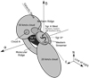 |
Fig. 1 Sketch of the main features within the 200 × 200 arcsec2 region around the supermassive black hole Sgr A* shown by a star. The features indicated in gray correspond mostly to the molecular components. The Sgr A East SNR (black ellipse) and Sgr A West (black minispiral) are shown as well. The ionized Northern, Eastern, and Southern arms of Sgr A West are indicated. The big circle and ellipse represent the 50 and 20 km s−1 clouds, respectively. Both clouds seem to be connected by the Molecular Ridge (the curved streamer). The Western Streamer and the Northern Ridge are also shown. |
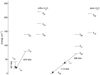 |
Fig. 2 Energy level diagram of ortho and para H2O. The observed ortho and para H2O transitions are shown with arrows. The frequencies of the observed H2O transitions are also indicated. |
2 Observations
The data were taken with the Heterodyne Instrument for the Far Infrared (HIFI) instrument (de Graauw et al. 2010) onboard the Herschel Space Observatory. Figure 2 shows the energy level diagram of the observed H2O transitions. We performed mapping observations of the ortho 556.936 GHz (557 GHz) 110 − 101, para 987.927 GHz (988 GHz) 202 − 111, and para 1113.343 GHz (1113 GHz) 111 − 000 transitions of H2O. We mapped an area of ~47 × 47 pc2 around Sgr A* using the OTF (On the Fly) observing mode, but in this paper we have focused on a region of ~8 × 8 pc2 centered at the position of the radio source Sgr A* ( = 17h45m40s.031, −29°00′28.′′58). We have also obtained OTF data of the ortho 1669.904 GHz (1670 GHz) 212 − 101 H2O transition, but due to the sensitivity only spectra for three selected positions around Sgr A* (see Table 1 and Fig. 3 for their positions) have been extracted in order to study the water excitation. Since the emission from the GC is very extended, the OTF maps were observed in position switching mode, with the reference observed towards the position α = 17h46m10s.42, δ = −29°07′08.′′04 (J2000).
We have also obtained single position observations of the ortho 547.676 (548 GHz) 110 – 101 and para 1101.698 (1102 GHz) 111 – 000 H O transitions towards the three selected positions in the vicinity of Sgr A*, where the 212 – 101 H2O spectra were extracted from the data cube. Table 2 lists the bands of the HIFI instrument where the H2O and H
 O transitions were observed. The two CND positions, CND1 and CND2, were observed in the southwest and northeast lobes, respectively, of the CND (see Fig. 6), and the third single position was observed towards the 20 km s−1 cloud. The reference position of the single position observations was the same as in the OTF observations. The observation dates and IDs of the OTF and single position observations are given in Table 2.
The raw data were processed using version 8 of the HIPE1 pipeline to a level 2 product. The baseline subtraction and gridding were done using the GILDAS software package2. The data were calibrated using hot and cold black body measurements. The intensity scale is the main beam brightness temperature (Tmb), obtained using the standard main beam efficiencies (ηmb), ηmb = 0.75 for the 110 − 101 H2O and H O transitions, ηmb = 0.74 for the 202 − 111 H2O, 111 − 000 H2O, and H
 O transitions, and ηmb = 0.71 for the 212 − 101 H2O transition. We resampled all spectra to a velocity resolution of 5 km s−1 appropriate for the linewidths around 20–100 km s−1 observed in GC sources. The half-power beam width (HPBW) at the observed H2O and H
 O frequencies is listed in Table 2. In our study we have also used Spectral and Photometric Imaging REceiver (SPIRE, Griffin et al. 2010) spectra observed with the SPIRE Short Wavelength (SSW) Spectrometer in February 2011. The SPIRE data (the observation ID is 1342214842) were also processed using the HIPE (version 8) pipeline to level 2.
Source positions.
3 Maps and spectra of H2O towards the 64 pc2 region around Sgr A*
The central panels in Fig. 3 show the integrated intensity maps of the three H2O transitions at 557, 988, and 1113 GHz. The three maps were obtained by integrating over the velocity range between −180 and +140 km s−1. In Fig. 3 we observe H2O emission and absorption features in the 557 and 1113 GHz maps, whereas only emission dominates the 988 GHz map. Unfortunately, the H2O map at 1113 GHz is affected by striping along the scanning direction due to standing waves, which originate from the local oscillator feed horns of HIFI as described in the HIFI handbook3. Our 1113 GHz data were affected by standing waves as the 1113 GHz water transition falls at the edge of the mixer band 4, where the standingwaves are more prominent (see Sect. 5.3 in the HIFI handbook). We have not been able to remove these standing waves in our data with our baseline subtraction or even applying the methods recommended in the HIFI data reduction guide4. Average spectra at 1113 GHz with standing waves (with amplitudes around 0.15 K) are shown in Fig. A.1, which have been extracted over parallelograms 1 and 2 drawn in the 1113 GHz H2O map shown in Fig. 3.
To study the physical conditions and the chemical composition of GC features, Amo-Baladrón et al. (2011) used seven representative positions selected from their SiO(2–1) emission maps. The positions are associated with the following features: (1) the southwestern CND (this position also covers the northern part of the 20 km s−1 cloud), (2) the northwestern CND, (3) the northeastern CND (this position also covers the 50 km s−1 cloud and the Northern Ridge), (4) the 50 km s−1 cloud (this position also covers Cloud A), (5) the Western Streamer north, (6) the Western Streamer south, and (7) the 20 km s−1 cloud. Figure 3 also shows line profiles of ortho 110 − 101, and para 202 − 111 and 111 − 000 H2O transitions extracted from the previous seven positions. All spectra at the three frequencies were extracted from H2O cubes convolved tothe 38′′ beam of HIFI at 557 GHz.
To identify the emission and/or absorption from GC features in Fig. 4, we have shown the spatial distribution of the water emission/absorption in the ortho 110 − 101 and para 202 − 111 H2O transitions integrated over ten velocity ranges. In this figure, para 111 – 000 H2O maps are not shown as the data cube suffers from standing waves, causing striping in the 1113 H2O maps. The 557 and 988 GHz maps are only slightly affected by striping (see Fig. 4). We have used the same velocity ranges in our velocity integrated intensity H2O maps as those used by Amo-Baladrón et al. (2011). In Fig. 4 the black crosses show the same positions associated with GC features as in Fig. 3, from where H2O spectra were extracted.
In Fig. 5 we have compared our ortho 110 − 101 and para 202 − 111 H2O maps with J = 2–1 emission maps of the shock tracer SiO (Martín-Pintado et al. 1997), obtained by Amo-Baladrón et al. (2011). For the comparison, previously the 988 GHz H2O and SiO(2–1) maps were convolved tothe 38′′ beam of the ortho 557 GHz H2O map.
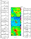 |
Fig. 3 Central panels: velocity integrated intensity maps of H2O at 557,988, and 1113 GHz. The beam sizes are shown in the left corner of each map. The maps at the three frequencies were integrated over the velocity range of [−180,+140] km s−1. The first contour levels for the H2O maps at 557 and 1113 GHz are at −3σ (black contour) for the absorption, 3σ (red contour) for the emission, but the 988 GHz line is at 3σ (red contour) for the emission. The steps are of 4.5 K km s−1 (−4.5 K km s−1 for the absorption) at 557 GHz and 26.0 K km s−1 (−26.0 K km s−1 for the absorption at 1113 GHz) at 988 and 1113 GHz (σ = 4.1, 11.3, and 9.6K km s−1 at 557, 987, and 1113 GHz, respectively). Sgr A* is shown with a black star and it is the origin of the offsets. Black crosses and their numbers show the positions where spectra of the left and right panels were extracted. Every position is associated with a representative GC feature (see below). The three positions where the H |


Observations of H2O and H O.
O.
3.1 Analysis of the H2O spectra
We have noted in Fig. 3 that the ortho 110 − 101 and para 111 – 000 H2O lines are absorption-dominated in almost all positions, while the para 202 − 111 H2O lines are emission-dominated in all positions. Most spectra from the ground state ortho 110 − 101 and para 111 − 000 H2O transitions reveal the presence of narrow absorption features at V LSR = 0, −30, −55 km s−1 , as well as a broad absorption feature at approximately −130 km s−1. The absorption features at 0, −30, and −55 km s−1 have been associated with the Local Sgr, −30 km s−1 and 3-kpc Galactic Arms, respectively, and the broad absorption at −130 km s−1 with the Molecular Ring located ~180 pc around the GC (Sandqvist et al. 2003).
The CND and the 20 km s−1 cloud have been studied by Amo-Baladrón et al. (2011) using the emission from SiO, H13 CO+, HN13C, HNCO, C18O, and CS. Based on that study, we expect that the water emission towards the CND1 and CND2 positions could be affected by water emission or absorption from the 20 and 50 km s−1 clouds in the velocity ranges of ~[−10,+40] and ~[+10,+70] km s−1, respectively, whereas the 20 km s−1 cloud position is not expected to be affected by water emission or absorption from any positive-velocity source along this line of sight. These three positions are indicated in Fig. 3. In fact, we have seen in Fig 3 that the ortho 110 − 101 and para 202 − 111 water line profiles of positions 2 and 3, which are close to our CND2 position, reveal signs of contribution in the water emission from the 50 km s−1 cloud. We have also noted in Fig. 3 that the water line profiles of position 1, which coincides with our CND1 position, would be affected by water emission or absorption from the 20 km s−1 cloud. Additionally, we have seen in Fig. 3 that the water line profiles of position 7, located around 57′′ northeast from our 20 km s−1 cloud position, are not affected by water emission or absorption from other positive-velocity line of sight sources.
3.2 Analysis of the 110 − 101 H2O emission/absorption distribution towards GC sources
As seen in Fig. 4, at 557 GHz absorption features are observed from −220 to 10 km s−1. The emission at 557 GHz covers the velocity range [−95,130] km s−1. The absorption features at 557 GHz within the velocity range of [−220,+10] km s−1 correspond to the Local Sgr, −30 km s−1, 3-kpc Arms, and the Molecular Ring. We have found that the ortho 110 − 101 H2O emission peaks in the extreme blue-shifted velocity range of [−95, −20] km s−1 in the southwestern CND, as well as at the extreme red-shifted velocity range of [+70,+130] km s−1 in the northwestern and the northeastern CND. Ortho 110 − 101 H2O emission is not detected in Cloud A at the velocity range of [−95, −50] km s−1 likely due to the 3-kpc arm absorption (see spectra of position 4 in Fig. 3). In the velocity ranges of [+25,+40] and [+40,+70] km s−1 we have detected ortho 110 − 101 H2O emission from the 20 and 50 km s−1 clouds, respectively. We have also detected ortho 110 − 101 H2O emission towards the Western Streamer south and Western Streamer north in the velocity ranges of [−50, −20] and [+10,+25] km s−1, respectively. Ortho 110 − 101 H2O emission is not detected in the Northern Ridge at the velocity range of [−20,+10] km s−1, probably due to the absorption at ~0 km s−1 by the Local Sgr Arm (see spectra of position 3 in Fig. 3). Moreover, Fig. 5 shows a very good agreement between the emission of SiO(2–1) and ortho 110 − 101 H2O in the CND, Western Streamer, and the 20 and 50 km s−1 clouds.
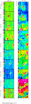 |
Fig. 4 Integrated intensity maps of H2O at 988 GHz (first row) and 557 GHz (second row). The velocity ranges are indicated at the top of each column. The first contour levels of H2O (557 GHz) are at −3σ (blue contour) for the absorption, 3σ (white contour) for the emission in steps of 1.5 K km s−1 (−1.5 K km s−1 for the absorption, σ in the range 1.0–1.5 K km s−1 for all velocity ranges). The first contour levels of H2O (988 GHz) are at 3σ (white contour) for the emission in steps of 7 K km s−1 (σ in the range 2.0–3.5 K km s−1 for all velocity ranges). The wedge above each panel shows the H2O integrated intensity scale given in K km s−1. The black star represents Sgr A* and the origin of the offsets in arcsec. Black crosses and their numbers show positions associated with GC sources labeled in the H2O maps at 557 GHz. Spectra from those positions are shown in Fig. 3. Beam sizes (38′′ at 557 GHz and 22′′ at 988 GHz) are shown in the left corner of the first column. |
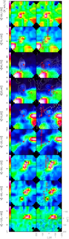 |
Fig. 5 Comparison between the SiO(2–1) maps (background images) obtained by Amo-Baladrón et al. (2011) and our H2O maps at 988 GHz (first row) and 557 GHz (second row). The velocity ranges are indicated at the top of each column. The wedges at the top of the first row show the SiO(2–1) intensity gray scale in K km s−1. H2O contour levels (in blue and white for the absorption and emission, respectively) start at 3σ (−3σ) for the emission (absorption) at the two H2O frequencies, and they increase in 5σ (−5σ) and 4σ steps at 557 and 988 GHz, respectively. The red star represents Sgr A* and origin of the offsets in arcsec. Crosses and their numbers show positions associated with GC sources labeled in the second row. H2O spectra fromthose positions are shown in Fig. 3. The water and SiO(2–1) maps have the same beam size of 38′′ shown in the left corner of the first column. |
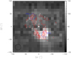 |
Fig. 6 Comparison between the integrated intensity maps of 988 GHz H2O in gray and CN(2–1) (contours, Martín et al. 2012). The integrated velocity range of the H2O map is [−180,140] km s−1. The wedge at the right shows the H2O intensity gray scale in K km s−1. Crosses and their numbers show positions, where spectra used in the kinematic study were extracted over the 22′′ beam. Thesepositions correspond to selected CN(2–1) and H2CO(330–220) emission peaks on the CND (Martín et al. 2012). The white star shows the position of Sgr A* and origin of the offsets. The HIFI beam of 22′′ at 988 GHz is shown in the left corner. Contour levels of the CN map start at 3σ and increase in 4σ steps. Blue circles with a size of 22′′ show the CND1 and CND2 positions selected for our study of the water excitation (see Sect. 5). The CND1 and CND2 positions were observed towards the southwest and northeast lobes, respectively, of the CND (Requena-Torres et al. 2012). |
3.3 Analysis of the 202 -111 H2O emission distribution towards GC sources
As mentioned above, the para 988 GHz H2O line only shows emission (see Figs. 3 and 4). This emission is concentrated in all previously mentioned GC features except in Cloud A and the Northern Ridge. Roughly the para 202 − 111 H2O emission exhibits a good correlation with the SiO(2–1) emission arising from GC sources in the vicinity of Sgr A* (see Fig. 5). In Fig. 6 we have compared the interferometric map of CN(2–1) (Martín et al. 2012) with the para 202 − 111 H2O emission map of the CND. Despite the difference in the spatial resolution between both maps, it can be clearly seen that there is an excellent correlation between the emission of the CN(2–1) and the para 202 − 111 H2O emission towards the southwestern CND.
3.4 Detection of H2O and H O in selected GC positions
In Fig. 7 we show the H O spectra, as well as the H2O spectra extracted from the data cubes for the CND1, CND2, and 20 km s−1 cloud positions indicated in Fig. 3. We have detected emission of the ortho 110 – 101 H
 O transition towards the CND, but unfortunately this transition is blended with the 13 CH3OH(162 − 161) line (this line is due to the HIFI double sideband) for the 20 km s−1 cloud position. Moreover, emission or absorption of the para 111 − 000 H
 O transition for the three studied positions was not detected with our sensitivity. Other molecular spectral features were found in the spectra of ortho 110 – 101 and para 111 − 000 H
 O transitions (see Fig. 7). Given our spectral sensitivity, the emission or absorption of the ortho 212 − 101 H2O transition (unfortunately this transition falls at the edge of the observed band) was not detected towards the CND and 20 km s−1 cloud positions, while the ortho 110 − 101, and para 202 − 111 and 111 − 000 H2O transitions reveal emission and/or absorption for the three studied positions. These H2O and H
 O spectra will be used in our study of the water excitation in Sect. 5.
4 Water kinematics
We have studied the CND kinematics of water vapor using the para H2O emission at 988 GHz since it is the least affected by absorption (see Figs. 3 and 4). This transition also exhibits significant emission arising from the Western Streamer, and the 20 and 50 km s−1 clouds as seen in Fig. 4. To derive the kinematics, we selected 220 − 111 H2O spectra (seeFig. 8) corresponding to the CN(2–1) and H2 CO(303 − 220) emission peaks studied by Martín et al. (2012). They found that the CN(2–1) emission is an excellent tracer of the CND, while the H2 CO(303 − 220) emission traces a shell-like structure where Sgr A East and both clouds seem to be interacting. Figure 6 shows the selected positions for the kinematic study superimposed on the para 220 − 111 H2O map. Positions 1–8 correspond to CN(2–1) emission peaks, while positions 9–12 correspond to H2 CO(303 − 220) emission peaks. Gaussian fits to the water para 220 − 111 line profiles were performed (see Fig. 8) and the derived parameters are shown in Table 3. The LSR (local standard of rest) velocities as a function of position angles (PA) are represented in Fig. 9. The PA is measured east from north centered on Sgr A*.
To describe the water kinematics from the CND, Fig. 9 shows the model prediction of the LSR velocities of a rotating ring model with an inclination of 75°, a position angle of 196°, and a rotation velocity vrot /sin i = 115 km s−1 of our best fit for the CND components (triangles). Our derived inclination angle, PA, and rotation velocity are slightly lower than those estimated by Martín et al. (2012) for the southwest lobe of the CND. Our derived three parameters are in agreement with those of rotating rings used to model the CND kinematics in Goicoechea et al. (2018b).
Limited by the Herschel spatial resolution, Fig. 9 shows the presence of four kinematically distinct structures around Sgr A* : the CND, represented by filled triangles, the 50 km s−1 cloud, represented by open squares, the 20 km s−1 cloud, indicated by filled squares, and the Western Streamer, represented by open circles. The 50 and 20 km s−1 clouds and the Western Streamer are located on top of the CND (Martín et al. 2012). The presence of more than one velocity component toward position 3, 5, 7, and 12 can be clearly seen in the 988 GHz spectra shown in Fig. 8. The velocity components of −40 and 53 km s−1 observed in position 3 are consistent with those arising from the southern and northern parts, respectively, of the Western Streamer (Amo-Baladrón et al. 2011). As shown in Fig. 9, there are three features not described by the rotating ring model, the 20 km s−1 and 50 km s−1 clouds and the Western Streamer. However, the 60 km s−1 velocity component of position 7 could be associated with the CND rather than with the 50 km s−1 cloud. Our result is consistent with that of Martín et al. (2012), who found kinematically distinct features in the vicinity of the CND using the CN(2–1) emission and indicating that the water emission traces both components, the CND and the clouds interacting with the SNR Sgr A East.
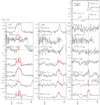 |
Fig. 7 Observational and simulated H2O and H |


5 Modeling the H2O and HO spectra and the continuum using a non-local radiative transfer code
We have used a non-local radiative transfer code (González-Alfonso et al. 1997) to model the H2O and H O line profiles observed with HIFI for the CND1, CND2, and the 20 km s−1 cloud positions, as well as to predict the infrared continuum observed with SPIRE for both CND positions. The numerical code solves the non-LTE equations of statistical equilibrium and radiative transfer in spherical geometry with an assumed radius. The sphere is divided into a set of shells defined by the number of the radial grid points. The physical conditions (water abundance
  , H2 density
  , kinetic temperature Tk , dust temperature Td , microturbulent velocity V t , and dust-to-gas mass ratio D/G) are defined in each shell of the spherical cloud, and we have assumed uniform physical conditions for simplicity. The numerical code convolves the emerging H2O line intensities to match the angular resolution of the HIFI instrument and the predicted continuum flux is integrated over the source. We have modeled the dust continuum flux by assuming that the source size is equal to the beam size at 250 μm. In addition to the collisional excitation, the code also accounts for radiative pumping through the dust emission, characterized by the Td , the dust opacity τd (González-Alfonso et al. 2014), and the D/G.
We ran two-component models to reproduce the H2O and H O line profiles for both CND positions using two fixed values of
  and Tk inferred by Requena-Torres et al. (2012), who explained the CO excitation in the CND with two components, one with Tk of ~200 K and
  of ~3.2 × 104 cm−3 for the low-excitation, and the second with warmer Tk of ~300–500 K and
  densities of ~2 × 105 cm−3 for the high-excitation component. The two model components are run separately, and the output line profiles are combined at each position. The V t, Td , and
  were considered free parameters and were changed to fit the observed water line profiles, with the Td giving an appropriate fit to both the continuum dust emission and the water line intensities of both CND positions.
For the modeling of the water line profiles for the 20 km s−1 cloud position, we considered a model with fixed  of 4 × 104 cm−3 (Amo-Baladrón et al. 2011) and Tk of 100 K (Hüttemeiser et al. 1993; Rodríguez-Fernández et al. 2001). We adopted a Td of 26 K for the 20 km s−1 cloud position as a compromise value between the Td inferred by Pierce-Price et al. (2000) and Rodríguez-Fernández et al. (2004) for the GC. The V t and
  were modified to fit the water lines for the 20 km s−1 cloud position.
The V t parameter was fixed in the modeling when a V t value provided thebest fit to the H2O line widths. The adopted  were varied until a good match to the water line intensities observed with Herschel/HIFI was obtained. When we fix n
 and vary
  , the line intensities depend on the source size. Details on the physical parameters are discussed in Appendix B.
It is well know that microturbulent approaches for line formations yield self-absorbed line profiles for optically thick lines (e.g., Deguchi & Kwan 1982), which is not observed in our data even for the very optically thick H2O 110 − 101 lines. In order to avoid such self-absorption, we have used a coarse grid such that the emergent line shapes of very optically thick lines are flat-top. While this has little effect on the emergent line fluxes (less than 40% for the H2O 110 − 101 line), our modeling is mostly based on the less optically thick H O 110 − 101 line for which the adopted grid is found to be irrelevant (see below). For all models we have included ten H2O lower rotational levels. We have also assumed that the H2O and H
 O molecules have uniform distributions and coexist with dust, and that the ortho to para H2O ratio (O/P) is the typical value of 3. In addition, the H
 O abundance relative to H2O is 1/250, which accords with the 16 O/18O isotopic ratio inferred for the GC (Wilson & Rood 1994). In our models the D/G was fixed to the typical value of 1%.
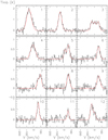 |
Fig. 8 Water 202-111 line profiles (black histogram) observed towards 12 positions (indicated in Fig. 6) on the CND. Gaussian fits to the water lines are shown with a red line. To fit the water line profiles, we have used a single Gaussian except in positions 3, 5, 7, and 12 (three Gaussians in position 3 and two Gaussians in positions 5, 7, and 12). |
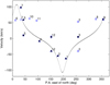 |
Fig. 9 LSR velocities of 988 GHz H2O lines for twelve positions on the CND (see Fig. 6) represented as a function of the PA. Different symbols represent several sources in the H2O map at 988 GHz: the CND (filled triangles), the 50 km s−1 cloud (open squares), the 20 km s−1 cloud (filled squares), and the Western Streamer (open circles). There are two velocity components in positions 5, 7, and 12, and three velocity components in position 3 (see text). The black dotted line represents our best fit of a rotating ring model to positions 1, 2, 4, 5, 7, 9, and 12. The error bars correspondto LSR velocity errors in the Gaussian fits. Error bars overlap with some symbols. The 5 km s−1 velocity component in position 3 and both velocity components in position 7 do not have error bars as the velocity was fixed in the Gaussian fit. |
Gaussian fit parameters of 998 GHz H2O lines on selected positions of the CND.
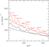 |
Fig. 10 Observational SPIRE spectra. The red and black histograms represent the SPIRE spectra for the CND1 and CND2 positions, respectively. The molecular lines in the SPIRE spectra correspond to CO and 13 CO lines. The red and black lines show the predicted dust continuum for the CND1 and CND2 positions, respectively, obtained using a two-component model (see text). |
5.1 Observational H2O and H O spectra and the dust continuum
As mentioned in Sect. 3.4, the ortho 110 − 101 and para 111 − 000 H O spectra were taken from the HIFI single position observations in the CND1, CND2 , and the 20 km s−1 cloud positions, while the ortho 110 − 101, 212 − 101 and para 202 − 111, 111 − 000 H2O spectra were extracted for the three positions from the data cubes. These spectra are shown in Fig. 7. As mentioned in Sect. 3, the H2O spectra at 1113 GHz are affected by standing waves with amplitudes around 0.15 K (see Fig. A.1). These artifacts do not affect our analysis of the CND1 position because the intensityof the 111 − 000 water line is at least a factor of five more intense than the amplitude of the artifact. Toward the CND2 and 20 km s−1 positions, the observed intensity of the 111 − 000 water line could be increased or decreased at most in 0.15 K due to the standing waves, however these possible changes do not affect our best fits for the water line profiles described below.
The SSW SPIRE data were used to extract spectra for the CND1 and CND2 positions. These spectra are shown in Fig. 10. Unfortunately, our SPIRE observations did not cover the 20 km s−1 cloud position, thus the continuum is not available for this position. Because of the limited spectral resolution of the SPIRE spectra, only CO and 13 CO transitions within J = 8–12 can be clearly distinguished in the spectra shown in Fig. 10.
5.2 Results
We find that, for both the low-density and the high-density model components, the H O 110 − 101 line is optically thick but effectively optically thin (Snell et al. 2000), so that its flux can be accurately estimated from
  , where Clu is the collisional excitation rate from the lower to the upper energy level, V is the volume of the source, and D is the distance. Our best-fit model provides a good match to the line with X
 = 4 × 10⁻⁸ for the high-density component of the CND2 position, which dominates the emission, and also yields fluxes for the H2O lines that are consistent with data. By using the above equation, we derive a flux for the H
 O 110 − 101 line of 2.6 × 10⁻¹⁵ erg s−1 cm−2 for the high-density component of the CND2 position, which is only a factor 1.2 higher than that estimated with our model. Such small differences are also found in the cases of the CND1 and the 20 km s−1 cloud positions. The H2O 110 − 101 line is not effectively thin, hence showing a flux significantly weaker than 250 × F(ortho H
 O 110 − 101).
We haveused the χ2 statistic in order to measure the goodness of fit of the data to the model for both CND positions. In Table 4 we show the results of a χ2 test in a two-component approach, showing only X and Td combinations that provide the lowest χ2 values for model fits to the H2O line intensities. The fitting of the dust continuum emission is checked after the χ2 testing. The χ2 statistic was run for the ranges X
 = 1 × 10⁻⁷–9 × 10⁻⁵ and Td = 15–55 K. The derived Td values in bold printin Table 4 give the best fits to the dust continuum emission of the CND positions (see Fig. 10). These Td values in combination with X
 values provide the lowest χ2 value for the CND1 position, but this does not happen in the case of the CND2 position. There are two combinations giving a χ2 value equal to 4.4 in the CND1 position, but that with the inferred Td = 45 K (for the low-density component) is the one that provides the best fit of the dust continuum. A χ2 value equal to 6.5 is the lowest value in the CND2 position, but in this case thederived Td = 40 K of the low-density component overestimates the observed dust continuum. Table 5 summarizes the physical conditions and parameters that provide the best fits of the data.
5.2.1 CND1 position
For the CND1 position we have found the best fit for the water line profiles (red histograms in Fig. 7) with the derived  of 9.3 × 10⁻⁶ and the derived Td of 45 K for the low-density component, and with the derived
  of 6.7 × 10⁻⁶ and the derived Td of 30 K for the high-density component. The inferred V t of 23 km s−1 provides the best fits to the H2O line widths.
As mentioned above, the observed ortho 110 − 101 and para 111 − 000 H2O line profiles at negative velocities towards the CND1 position are affected by absorption from foreground sources. To model these absorptions, we have considered spherical shells around the modeled sources, with a water abundance around 3 × 10⁻⁸ as derived for the −30 km s−1 spiral arm (Karlsson et al. 2013), and H2 densities of 103 cm−3 and kinetic temperatures of 50 K (Greaves & Williams 1994). Turbulent velocities of 1–2 km s−1 were appropriate to simulate those lines. Water lines are also affected by absorption toward nearby galaxies (Liu et al. 2017). The narrow absorption lines superimposed on top of the emission water lines create emission spikes observed in the 110 − 101 and 111 − 000 H2O lines. There is a very good overall agreement between the observations and the modeling. However, as expected for the complexity of the H2O excitation, there are differences in the intensity of the modeled and the observed spikes likely due to the assumed line-shape in the modeling. This difference is also seen in the case of the H2O 202 − 111 line.
Considering an optically thin regime, a dust-to-gas ratio of 1%, and a mass-absorption coefficient of 8.2 cm2 g−1 at 250 μm, the τd (250 μm) is related to the H2 column density as  /τd(250 μm) = 3.6 × 1024 cm−2. Based on the τd (250 μm) predicted with our two-component model (see Table 5), we have derived a H2 column density
  of 3.0–3.9 × 1022 cm−2 for the CND1 position, values listed in Table 5, together with the water abundances, turbulent velocities, dust temperatures, and dust opacities. For this model we have also derived H2O column densities (
 ) around 3 × 1017 cm−2 also included in Table 5. A total gas mass of 238 M⊙ is derived for the CND1 position by considering the N
 and the source size. This mass is a factor 1.6 lower than that estimated in Requena-Torres et al. (2012) for this position, which is reasonable given the simplicity of our modeling.
Lowest χ2 values for two-component model fits to the H2O line intensities.
5.2.2 CND2 position
For the CND2 position we have found the best fits for the water line profiles (red histograms in Fig. 7) with the derived  as 1.3 × 10⁻⁶ and the derived Td of 15 K for the low-density component, and with the derived
  as 13.3 × 10⁻⁶ and the derived Td of 25 K for the high-density component. The H2O line widths observed towards this position are fitted better with the derived V t of 14 km s−1. The modeling of the water lines of this position is complex because toward this line of sight the emission arising from the CND and the 50 km s−1 cloud is blended as discussed before. In Fig. 6 of Amo-Baladrón et al. (2011) we can clearly see that the CS(1–0) line emission arising from the western edge of the 50 km s−1 cloud that reaches velocities up to ~80 km s−1 is detected in the northeastern CND, the region that coincides with our CND2 position. An H2O abundance of 2 × 10⁻¹⁰ accounts for the emission or absorption contribution from the 50 km s−1 cloud in this CND position. We have simulated this cloud with a spherical symmetry, an
  of 3 × 105 cm−3, a Tk of 100 K, and a low Td of 20 K (Amo-Baladrón et al. 2011; Rodríguez-Fernández et al. 2001, 2004). The simulated 50 km s−1 cloud creates an absorption feature in the modeled 111 − 000 and 212 − 001 H2O lines (see Fig. 7). There is also a small difference between the modeled and observed para 111 − 000 H2O line intensity at ~100 km s−1 (see Fig. 7). This difference could be caused by either standing waves or the simplicity of spherical symmetry in our models.
Following the same procedure as for the CND1 position, based on τd (250 μm) we have estimated a  of 3.2–3.6 × 1022 cm−2 for the CND2 position. We have also determined
  of 4.1 × 1016 cm−2 for the low-density component and of 4.8 × 1017 cm−2 for the high-density component. The whole set of the derived parameters obtained using our model are listed in Table 5. The derived
  yield a total gas mass of 253 M⊙ that is comparable to the mass obtained by Requena-Torres et al. (2012) for this position.
5.2.3 Position of the 20 km s−1 cloud
As already mentioned, we expect that the H2O emission toward the 20 km s−1 cloud position is not affected by contributions from other positive-velocity line of sight sources. We have searched for the best fits to the water line profiles varying only the  and V t, finding values of the
  of 4.0 × 10⁻⁸ and V t of 9 km s−1.
Figure 7 shows that all the modeled water line profiles in emission or absorption are in agreement with the observed line profiles, except in the case of the 110 − 101 H O spectrum, where the water line is blended with the emission from the 13 CH3OH(162 − 161) line. This argument is supported by the 110 − 101 H2O to H
 O line intensity ratio that is equalto ~50 at 110 km s−1 for the CND1 position, but as low as ~14 for the 20 km s−1 cloud position. The τd(250 μm) of 0.08 predicted for this position corresponds to the derived
  of 2.7 × 1023 cm−2. For this position we have derived an
  as 1.1 × 1016 cm−2 included in Table 5, where the other derived parameters are also summarized.
Parameters of the models for the three selected positions in the vicinity of Sgr A*.
6 Discussion
The derived free parameters together with the fixed parameters that provide the best fits to the water line profiles are given in Table 5. The derived X , Vt , and Td are dependent on the assumed source sizes, which are not very well known. However, the Vt of 9–23 km s−1 obtained for the three studied positions is consistent with those of 15–30 km s−1 derived towards the GC (Güsten & Philipp 2004). Furthermore, for the CND we have derived Td of 15–45 K, which agree quite well with the two dust components of 24 and 45 K reported by Etxaluze et al. (2011). The Td = 15
 K derived for the low-excitation component in the CND2 position is lower than that derived in the CND1 position. The derived Td of 45
 K in the CND1 position is responsible for pumping the 202 – 111 H2O line (see Sect. 6.1), which has an intensity a factor of four higher than that in the CND2 position.
The derived X within (0.1–1.3) × 10−5 for the CND and the derived X
 of 4.0 × 10⁻⁸ for the 20 km s−1 cloud are also consistent with the lower limit of 2 × 10⁻⁸ for X
 as calculated by Karlsson et al. (2013) for these two GC sources using the non-LTE radiative transfer code RADEX. The inferred N
 (3.0–3.9) × 1022 cm−2 for the CND are similar to those determined from CO in previous studies (Requena-Torres et al. 2012; Bradford et al. 2005) and also consistent with N
 1022–1023 cm−2 calculated from measurements of the HCN molecule (Güsten et al. 1987; Jackson et al. 1993). The derived N
 of 2.7 × 10²³ for the 20 kms−1 cloud is slightly higher than that of ~7 × 1022 cm−2 derived by Rodríguez-Fernández et al. (2001) using 13CO. On the other hand, our derived value of N
 is lower than that of ~7 × 1023 cm−2 estimated from the ground-state transition of H13CO+ for this cloud (Tsuboi et al. 2011).
6.1 Excitation of water
For the CND1 position, we have found that water excitation is affected by the dust emission, since when we removed the dust effects in our model, the observed ortho 110 − 101 H2O and H O line intensities were slightly overestimated, the observed para 202 − 111 H2O line intensity was underestimated by a factor of ~2 due to the lack of radiative pumping, while the other modeled water lines remain unchanged. The 202 − 111 H2O line is also found to be pumped through absorption of continuum photons in extragalactic sources (Omont et al. 2013). For the CND2 position, there is no strong radiative excitation from the dust emission of the para 202 − 111 H2O line as all predicted water line intensities remain unaffected. Therefore, only collisional excitation is responsible for the 202 − 111 H2O line strength.
For the 20 km s−1 cloud position, we have noted that all four H2O and the two H O lines are also affected by radiative excitation from dust, since all predicted water line profiles changed significantly when dust effects were removed in the modeling, with the observed ortho 110 − 101 and para 202 − 111 H2O line intensities being overestimated and underestimated by a factor of ~2, respectively, due to the lack of dust effects. Therefore, in the CND1 and the 20 km s−1 cloud positions the water excitation is determined by collisional effects and absorption of far-infrared continuum photons, while radiation is not important in the water excitation of the CND2 position.
6.2 Chemistry and heating
We have derived a X of 1.3
 10−5 for the high-density component of the CND2 position, a value that is ten times higher than that derived for the low-density component of the same position. For both density components of the CND1 position, we have inferred X
 within (6.7–9.3) × 10−6.
As already mentioned, Amo-Baladrón et al. (2011) found that the shock tracer SiO revealed high abundances in the CND, where in contrast the HNCO showed the lowest abundances due to its photodissociation by UV photons. The spatial correlation between thewater and SiO(2–1) emission in the CND (see Sects. 3.2 and 3.3) points towards grain sputtering as an important mechanism for gas phase water production in the CND. We have derived Tk ∕Td ratios in therange of 4–17 for the CND, which also supports the idea that mechanical energy from shocks plays a role in the H2O chemistry.
Harada et al. (2015) studied the chemical composition of the southwest lobe of the CND (our CND1 position) through chemical modeling. Their model considers high temperature chemistry and mimics grain sputtering by shocks and the effects of cosmic rays. They also studied the effects of UV photons in the chemistry, finding that the abundances of many molecules are not affected in AV < 1 regions while the H3 O+ (that can form H2O via its dissociative recombination; Vejby-Christensen et al. 1997) and HCO+ abundances can reach values up to 10−8 for AV < 1 regions. The n and Tk of the low-density CND components agree with those modeled by Harada et al. (2015) for gas with a preshock density of 2 × 104 cm−3, a shock velocity of 10 km s−1 , and timescales around 102.8 yr after the shock (hereafter scenario 1), while the n
 and Tk of the high-density CND components is in agreement with those modeled for a shocked medium with a preshock density of 2 × 105 cm−3, shock velocities of 10–20 km s−1 , and timescales around 101.2−1.4 yr (hereafter scenario 2).
The X of (0.7–1.3) × 10−5 derived for the high-density components of the CND is a factor of 15–29 lower than that of about 2 × 10⁻⁴ predicted in scenario 2. Varying cosmic-ray ionization rates within 10−17–10−13 s−1 does not change the X
 predicted in scenario 2 (see Fig. 5 of Harada et al. 2015). The above difference can be decreased (within a factor of 9–22) when the errors in our estimates are considered. Our X
 of (0.7–1.3) × 10−5 are consistent with those predicted in scenario 2 but with timescales of 104 yr and a cosmic-ray ionization rate of 10−14 s−1 and assuming that there might have been multiple shocks. This is also in good agreement with the n
 and Tk of the high-density CND components predicted by the models in Harada et al. (2015). The value of 10−14 s−1 for the cosmic-ionization rate is also consistent with those derived for sources located within the Central Cluster (Goto et al. 2014).
On the other hand, the X of 9.3 × 10⁻⁶ estimated for the low-density component of the CND1 position is only a factor two lower than that predicted in scenario 1, with a preshock density of 2 × 105 cm−3 and a cosmic-ray ionization rate of 10−16 s−1 (hereafter modified scenario 1). The X
 of 1.3 × 10⁻⁶ derived for the low-density component of the CND2 component is 15 times lower than that predicted in modified scenario 1. A cosmic-ionization rate of 10−14 s−1 decreases the water abundance at timescales around 103 yr, giving a better agreement with our derived water abundances for both low-density CND components in the modified scenario 1.
It is considered that around 14 and 18% of the high- and low-density material, respectively, of the CND could be considered as a photon-dominated region (PDR) with AV < 5 given their H2 densities and source sizes. The far-ultraviolet radiation field is G0 ~ 105 in the inner edge of the CND (Burton et al. 1990). Using a chemical model, Hollenbach et al. (2009) derived X of ~10−7 for molecular clouds affected by a far-ultraviolet flux of G0 < 500. However, for G0 > 500 and the gas density of 104 cm−3 this model predicted a peak X
 around 10−6 only at AV = 8 due to thermal desorption of O atoms and subsequent water production through neutral-neutral reactions, while at AV < 5 the water is photodissociated and its abundance decreases below 10−8. In PDRs the N
 are ~ 1015 cm−2 (Hollenbach et al. 2009), which are lower than those derived in the CND at least by a factor of ~41 (see Table 5). The only effect of increasing G0 in the modeling is that the H2O shell penetrates further into the cloud, while the H2O column densities remain constant (Hollenbach et al. 2009). From this comparison, PDRs do not seem to play a role in the water chemistry in the CND.
In addition, CO/H2O abundance ratios have been used to establish if there is any PDR contribution to the water emission. The starburst galaxy M 82 revealed CO/H2O ~ 40 (Weiss et al. 2010). The CO lines are a factor of ≳50 stronger than the H2O lines in the prototypical galactic PDR Orion Bar (Habart et al. 2010), which is in contrast to what is observed in Mrk 231, where the H2O and CO lines are comparable (González-Alfonso et al. 2010). Based on the integrated intensities of 13 CO lines with J = 2–1, 6–5, 13–12 obtained by Requena-Torres et al. (2012), we have derived CO to H2O(210 − 111) integrated line intensity ratios in the range of 4–43 for the CND. The 13 CO data have a similar angular resolution to our H2O(210 − 111) data and the 13CO can be converted to12CO by assuming a 12 C/13C = 20 ratio, typical for the CG (Wilson & Rood 1994). Our highest CO/H2O ratio of 43, similar to that of M 82, could indicate that there is some PDR contribution in the water chemistry of the CND. This result is in contrast to the suggestion found in the previous discussion. A hot CO component found toward the central cavity is heated by a combination of UV photons and shocks (Goicoechea et al. 2013).
Apparently the Tk < 200 K of the low-density CND components are not high enough for water production through neutral-neutral reactions, which activate at Tk > 300 K (Neufeld et al. 1995), however, high-temperature chemistry of water could be produced at the shock fronts of the low-density CND components with warmer gas (>300 K) and of course in the high-density CND components with Tk > 325 K. As mentioned, the high-temperature chemistry is considered in the modeling by Harada et al. (2015). On the other hand, the Td < 45 K derived in the CND rules out thermal evaporation of H2O because thismechanism needs grain temperatures around 100 K (Fraser et al. 2001).
It is thought that the effects of X-rays in the CND chemistry are negligible as the X-ray ionization rate is lower than 10−16 s−1 at H2 column densities >1021 cm−2 (Harada et al. 2015). This is consistent with the results of Goicoechea et al. (2013), who found that X-rays do not dominate the heating of hot molecular gas near Sgr A*.
The X of ~4.0 × 10⁻⁸ derived in the 20 km s−1 cloud is at least a factor of ~33 smaller than those derived in the CND, suggesting that the water freeze-out can partially account for the low X
 . In these regions the water could be produced through an ion-neutral chemistry (Vejby-Christensen et al. 1997). It would be interesting to consider if the modeling proposed by Harada et al. (2015) including cosmic-ray chemistry without shocks would predict the low water abundance derived in the 20 km s−1 cloud. In summary, the X
 within (0.1–1.3) × 10−5 derived in the CND are better explained in scenarios that consider grain sputtering by shocks of 10–20 km s−1, cosmic rays, and high-temperature chemistry, with a possible contribution of PDR chemistry, while the water freeze-out seems to be responsible for the low X
 of 4.0 × 10⁻⁸ derived for the 20 km s−1 cloud.
7 Conclusions
We presented velocity-integrated ortho 110 − 101, and para 202 − 111 and 111 − 000 water maps of an area of ~8 × 8 pc2 around Sgr A* observed with the Herschel Space Telescope. The velocity-integrated ortho 110 − 101 and para 111 − 000 H2O maps reveal emission and/or absorption, whereas the para 202 − 111 H2O maps revealonly emission. The ground-state ortho water maps show emission in the velocity range of [−95,130] km s−1 associated with the CND, the Western Streamer, and the 20 and 50 km s−1 clouds. Thiswater emission from the southwestern CND and the Western Streamer south is substantially absorbed by foreground sources. The ground-state ortho water maps show absorption structures in the velocity range of [−220,10] km s−1 associated with foreground sources.
The para 202 – 111 water emission is concentrated towards the CND, the Western Streamer, and the 20 and 50 km s−1 clouds. Based on the lack of absorption of the para 202 – 111 water emission around the black hole Sgr A*, we used this emission in a velocity versus position angle diagram, finding that the para 202 – 111 water emission traces the CND and the clouds that are interacting with the SNR Sgr A East.
Using a non-local radiative transfer code, we derived X of ~(0.1–1.3) × 10−5, Vt of 14–23 km s−1, and Td of 15–45 K for the CND, and X
 of 4.0 × 10⁻⁸ and Vt of 9 km s−1 for the 20 km s−1 cloud. From this study, we also found that collisions and dust effects can account for the observed water excitation in the CND1 and the 20 km s−1 cloud positions, but there is no need for radiative excitation in the CND2 position.
We propose that the gas phase water vapor production in the CND is produced by a combination of grain sputtering by shocks of 10–20 km s−1, high-temperature and cosmic-ray chemistries, plus a probable PDR chemistry, whereas the low X derived in the 20 km s−1 cloud could be a consequence of the water freeze-out.
Acknowledgements
J.M.-P. and E.G.-A. acknowledge partial support by the MINECO and FEDER funding under grants ESP2015–65597–C4–1 and ESP2017–86582–C4–1–R. A.H. acknowledges support for this work by NASA through an award issued by JPL/Caltech. E.G.-A. is a Research Associate at the Harvard–Smithsonian Center for Astrophysics. We thank the anonymous referee for the useful comments that improved the manuscript.
Appendix A Standingwaves in spectra
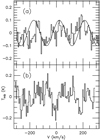 |
Fig. A.1 Panels a and b: average spectra extracted from parallelograms 1 and 2, respectively, shown in Fig. 3. The spectra are affected by standing waves, with a period around 200 km s−1, which originate from the local oscillator feed horns of HIFI (see Sect. 3). Panel a illustrates a sine function, highlighting the shape of the standing wave. |
Appendix B Physical parameters of the studied sources
B.1 Dust temperature and turbulent velocity
Pierce-Price et al. (2000) derived a fairly uniform dust temperature of 21±2 K over an extended region in the GC. Rodríguez-Fernández et al. (2004) derived Td < 30 K towards molecular clouds distributed along the central 500 pc region of the Galaxy. Additionally, Etxaluze et al. (2011) using PACS and SPIRE data found that two different components are required to explain the observed continuum in the CND, a hot component with a Td of 45 K and n of 1 × 104 cm−3 and a cold component with a Td of 24 K and n
 of 2 × 104 cm−3. They also found a very hot Td = 90 K that arises from the central cavity that was not covered by our CND observations. Therefore, this hot Td was not considered in our modeling. Güsten & Philipp (2004) derived Vt of 15–30 km s−1 toward GC clouds. Thus, in our models we explore values of Td of ~15–50 K and Vt of 15–30 km s−1.
B.2 Density of H2, kinetic temperature, and source size
Bradford et al. (2005) studied the CO excitation of one CND position (with offsets of Δα = −15′′ and Δδ = −30′′ from Sgr A*), which is close to our studied CND1 position. They used several CO rotational transitions in combination with a radiative transfer code to derive a Tk of 240 K and a n of 7.1 × 104 cm−3. The Tk and n
 derived by Bradford et al. (2005) are slightly higher than those derived by Requena-Torres et al. (2012) for the low-excitation gas of the CND. The n
 around 3 × 105 cm−3 derived for our two CND positions by Amo-Baladrón et al. (2011) agree well with the high-excitation component of Requena-Torres et al. (2012), who derived source radii around 0.32 pc and 0.07 pc for the low- and high-excitation components, respectively. Our two CND positions observed with HIFI coincide with the CND positions studied by Requena-Torres et al. (2012). The CND1 and CND2 positions are observed towards the southwest and northeast lobes, respectively, of the CND (see Fig. 6). As seen in Fig. 6, the interferometric emission map of CN(2–1) shows that one clump is found toward each CND position. The clumps in the CND1 and CND2 positions are identified as clumps Q and A, respectively, in the interferometric emission map of HCN(4–3) obtained by Montero-Castaño et al. (2009). Since CO usually traces the H2 column density, we assume a clump radius for the water emission for the CND1 and CND2 positions following the results obtained by Requena-Torres et al. (2012; see Table 5).
The velocity range of [10,40] km s−1 of the ortho 110 − 101 H2O map in Fig. 4shows the northern part of the 20 km s−1 cloud. For this core we have derived a size around 9 pc for the minor axis, which is somewhat larger than the 7.5 pc size derived by Zylka et al. (1990), but the 202 − 111 H2O maps show that the 20 and 50 km s−1 clouds (see Fig. 4) have source sizes a factor of ~2 more compact than those observed at 557 GHz. Therefore, for the modeling we assume a 20 km s−1 cloud with spherical symmetry and a size of 4.5 pc. Interferometric maps of ammonia observed by Coil & Ho (2000) reveal a size for the 20 km s−1 cloud relatively similar to that shown by the 202 − 111 H2O emission.
References
- Amo-Baladrón, M. A., Martín-Pintado, J., & Martín, S. 2011, A&A, 526, A54 [NASA ADS] [CrossRef] [EDP Sciences] [Google Scholar]
- Blum, R. D., Schaerer, D., Pasquali, A., et al. 2001, AJ, 122, 1875 [NASA ADS] [CrossRef] [Google Scholar]
- Boehle, A., Ghez, A. M., Schödel, R., et al. 2016, ApJ, 830, 17 [NASA ADS] [CrossRef] [Google Scholar]
- Bradford, C. M., Stacey, G. J., Nikola, T., et al. 2005, ApJ, 623, 866 [NASA ADS] [CrossRef] [Google Scholar]
- Burton, M. G., Hollenbach, D. J., & Tielens, A. G. G. M. 1990, ApJ, 365, 620 [NASA ADS] [CrossRef] [Google Scholar]
- Coil, A. L., & Ho, P. T. P. 2000, ApJ, 533, 245 [NASA ADS] [CrossRef] [Google Scholar]
- de Graauw, T., Helmich, F. P., Phillips, T. G., et al. 2010, A&A, 518, L6 [NASA ADS] [CrossRef] [EDP Sciences] [Google Scholar]
- Deguchi, S., & Kwan, J. 1982, ApJ, 260, 579 [NASA ADS] [CrossRef] [Google Scholar]
- De Pree, C. G., Goss, W. M., & Gaume, R. A. 1998, ApJ, 500, 847 [NASA ADS] [CrossRef] [Google Scholar]
- Etxaluze, M., Howard, A. S., Tolls, V., Stark, A. A., & González-Alfonso, E. 2011, ApJ, 142, 134 [NASA ADS] [CrossRef] [Google Scholar]
- Fraser, H. J., Collings, M. P., McCoustra, M. R. S., & Williams, D. A. 2001, MNRAS, 327, 1165 [NASA ADS] [CrossRef] [Google Scholar]
- Ferrière, K. 2012, A&A, 540, A50 [NASA ADS] [CrossRef] [EDP Sciences] [Google Scholar]
- Gaume, R. A., Claussen, M. J., De Pree, C. G., Goss, W. M., & Mehringer, D. M. 1995, ApJ, 449, 663 [NASA ADS] [CrossRef] [Google Scholar]
- Goicoechea, J.R., Etxaluze, M., Cernicharo, J., et al. 2013, ApJ, 769, L13 [NASA ADS] [CrossRef] [Google Scholar]
- Goicoechea, J.R., Santa-Maria, M. G., Teyssier, D., et al. 2018a, A&A, 616, L1 [NASA ADS] [CrossRef] [EDP Sciences] [Google Scholar]
- Goicoechea, J.R., Pety, J., Chapillon, E., et al. 2018b, A&A, 618, A35 [NASA ADS] [CrossRef] [EDP Sciences] [Google Scholar]
- González-Alfonso, E., & Cernicharo, J. 1997, A&A, 322, 938 [NASA ADS] [Google Scholar]
- González-Alfonso, E., Fischer, J., Isaak, K., et al. 2010, A&A, 518, L43 [NASA ADS] [CrossRef] [EDP Sciences] [Google Scholar]
- González-Alfonso, E., Fischer, J., Aalto, S., et al. 2014, A&A, 567, A91 [NASA ADS] [CrossRef] [EDP Sciences] [Google Scholar]
- Greaves, J. S.,& Williams, P. G. 1994, A&A, 290, 259 [NASA ADS] [Google Scholar]
- Goto, M., Geballe, T. R., Indriolo, N., et al. 2014, ApJ, 786, 96 [NASA ADS] [CrossRef] [Google Scholar]
- Griffin, M. J., Abergel, A., Abreu, A., et al. 2010, A&A, 518, L3 [Google Scholar]
- Güsten, R., & Philipp, S. 2004, The Dense Interstellar Medium in Galaxies, Springer Proceedings in Physics (Berlin: Springer), 91, 253 [CrossRef] [Google Scholar]
- Güsten, R., Genzel, R., Wright, M. C. H., et al. 1987, ApJ, 318, 124 [NASA ADS] [CrossRef] [Google Scholar]
- Habart, E., Dartois, E., Abergel, A., et al. 2010, A&A, 518, L116 [NASA ADS] [CrossRef] [EDP Sciences] [Google Scholar]
- Harada, N., Riquelme, D., Jiménez-Serra, I., et al. 2015, A&A, 584, A102 [NASA ADS] [CrossRef] [EDP Sciences] [Google Scholar]
- Harris, A. I., Jaffe, D. T., Silber, M., & Genzel, R. 1985, ApJ, 294, L93 [NASA ADS] [CrossRef] [Google Scholar]
- Herrnstein, R. M., & Ho, P. T. P. 2002, ApJ, 579, L83 [NASA ADS] [CrossRef] [Google Scholar]
- Herrnstein, R. M., & Ho, P. T. P. 2005, ApJ, 620, 287 [NASA ADS] [CrossRef] [Google Scholar]
- Ho, P. T. P., Ho, L. C., Szczepanski, J. C., et al. 1991, Nature, 350, 309 [NASA ADS] [CrossRef] [Google Scholar]
- Hollenbach, D., Kaufman, M. J., Bergin, E. A., & Melnik, G. 2009, ApJ, 690, 1497 [CrossRef] [Google Scholar]
- Hüttemeiser, S., Wilson, T. L., Bania, T. M., & Martín-Pintado, J. 1993, A&A, 280, 255 [NASA ADS] [Google Scholar]
- Jackson, J. M., Geis, N., Genzel, R., et al. 1993, ApJ, 402, 173 [NASA ADS] [CrossRef] [Google Scholar]
- Karlsson, R., Sandqvist, Aa., Hjalmarson, Å., et al. 2013, A&A, 554, A141 [NASA ADS] [CrossRef] [EDP Sciences] [Google Scholar]
- Koyama, K., Maeda, Y., Sonobe, T., et al. 1996, PASJ, 48, 249 [NASA ADS] [CrossRef] [Google Scholar]
- Maeda, Y., Baganoff, F. K., Feigelson, E. D., et al. 2002, ApJ, 570, 671 [NASA ADS] [CrossRef] [Google Scholar]
- Martín, S., Martín-Pintado, J., Montero-Castaño, M., Ho, P. T. P., & Blundell, R. 2012, A&A, 539, A29 [NASA ADS] [CrossRef] [EDP Sciences] [Google Scholar]
- Martín-Pintado, J., de Vicente, P., Fuente, P., & Planesas, P. 1997, ApJ, 482, L45 [NASA ADS] [CrossRef] [Google Scholar]
- Martín-Pintado, J., Rizzo, J. R., de Vicente, P., Rodríguez-Fernández, N. J., & Fuente, A. 2001, ApJ, 548, L65 [NASA ADS] [CrossRef] [Google Scholar]
- McGary, R. S., Coil, A. L., & Ho, P. T. P. 2001, ApJ, 559, 326 [NASA ADS] [CrossRef] [Google Scholar]
- Mills, E. A. C., Güsten, R., Requena-Torres, M. A., & Morris, M. R. 2013, ApJ, 779, 47 [NASA ADS] [CrossRef] [Google Scholar]
- Montero-Castaño, M., Herrnstein, R. M., & Ho, P. T. P. 2009, A&A, 695, 1477 [NASA ADS] [CrossRef] [Google Scholar]
- Morris, M., & Serabyn, E. 1996, ARA&A, 34, 645 [NASA ADS] [CrossRef] [Google Scholar]
- Neufeld, D. A., Bergin, E. A., Melnik, G. J., & Goldsmith, P. F. 2003, ApJ, 590, 882 [NASA ADS] [CrossRef] [Google Scholar]
- Neufeld, D. A., Lepp, S., & Melnick, G. J. 1995, ApJS, 100, 132 [NASA ADS] [CrossRef] [Google Scholar]
- Liu, L., Weiss, A., Perez–Beaupuits, J. P., et al. 2017, ApJ, 846, 5 [NASA ADS] [CrossRef] [Google Scholar]
- Oka, T., Nagai, M., Kamegai, K., & Tanaka, K. 2011, ApJ, 732, 120 [NASA ADS] [CrossRef] [Google Scholar]
- Omont, A., Yang, C., Cox, P., et al. 2013, A&A, 551, A115 [NASA ADS] [CrossRef] [EDP Sciences] [Google Scholar]
- Park, S., Muno, M. P., Baganoff, F. K., et al. 2004, ApJ, 603, 548 [NASA ADS] [CrossRef] [Google Scholar]
- Paumard, T., Genzel, R., Martins, F., et al. 2006, ApJ, 643, 1011 [NASA ADS] [CrossRef] [Google Scholar]
- Pierce-Price, D., Richer, J. S., Greaves, J. S., Holland, W. S., & Jennes, T. 2000, ApJ, 545, L121 [Google Scholar]
- Ponti, G., Terrier, R., Goldwurm, A., Belanger, G., & Trap, G. 2010, ApJ, 714, 732 [NASA ADS] [CrossRef] [Google Scholar]
- Requena-Torres, M. A., Güsten, R., Weiss, A., et al. 2012, A&A, 542, L21 [NASA ADS] [CrossRef] [EDP Sciences] [Google Scholar]
- Rodríguez-Fernández, N. J., Martín-Pintado, J., Fuente, A., et al. 2001, A&A, 365, 174 [NASA ADS] [CrossRef] [EDP Sciences] [Google Scholar]
- Rodríguez-Fernández, N. J., Martín-Pintado, J., Fuente, A., Wilson, T. L., & Wilson, T. L. 2004, A&A, 427, 217 [NASA ADS] [CrossRef] [EDP Sciences] [Google Scholar]
- Sandqvist, Aa., Bergman, P., Black, J. H., et al. 2003, A&A, 402, L63 [NASA ADS] [CrossRef] [EDP Sciences] [Google Scholar]
- Sjouwerman, L. O., Lindqvist, M., van Langevelde, H. J., & Diamond, P. J. 2002, A&A, 391, 967 [NASA ADS] [CrossRef] [EDP Sciences] [Google Scholar]
- Snell, R. L., Howe, J. E., Ashby, M. L. N., et al. 2000, ApJ, 539, L93 [NASA ADS] [CrossRef] [Google Scholar]
- Sonnentrucker, P., Neufeld, D. A., Gerin, M., et al. 2013, ApJ, 763, L19 [NASA ADS] [CrossRef] [Google Scholar]
- Terrier, R., Ponti, G., Bélanger, G., et al. 2010, ApJ, 719, 143 [NASA ADS] [CrossRef] [Google Scholar]
- Tsuboi, M., Tadaki, K., Miyazaki, A., & Handa, T. 2011, PASJ, 63, 763 [NASA ADS] [CrossRef] [Google Scholar]
- Vejby-Christensen, L., Andersen, L. H., Heber, O., et al. 1997, ApJ, 483, 531 [NASA ADS] [CrossRef] [Google Scholar]
- Wang, Q. D., Gotthelf, E. V., & Lang, C. C. 2002, Nature, 415, 148 [NASA ADS] [CrossRef] [PubMed] [Google Scholar]
- Weiss, A., Requena-Torres, M. A., Güsten, R., et al. 2010, A&A, 521, L1 [NASA ADS] [CrossRef] [EDP Sciences] [Google Scholar]
- Wilson, T. L., & Rood, R. T. 1994, ARA&A, 32, 191 [NASA ADS] [CrossRef] [Google Scholar]
- Yusef-Zadeh, F., & Wardle, M. 1993, ApJ, 405, 584 [NASA ADS] [CrossRef] [Google Scholar]
- Yusef-Zadeh, F., & Mehringer, D. M. 1995, ApJ, 452, L37 [NASA ADS] [CrossRef] [Google Scholar]
- Yusef-Zadeh, F., Braatz, J., Wardle, M., & Roberts, D. 2008, ApJ, 683, L147 [NASA ADS] [CrossRef] [Google Scholar]
- Zhao, J., Morris, M. R., Goss, W. M., & An, T. 2009, ApJ, 699, 186 [NASA ADS] [CrossRef] [Google Scholar]
- Zylka, R., Mezger, P. G., & Wink, J. E. 1990, A&A, 234, 133 [NASA ADS] [Google Scholar]
HIPE is a joint development by the Herschel Science Ground Segment Consortium, consisting of ESA, the NASA Herschel Science Center, and the HIFI, PACS, and SPIRE consortia.
All Tables
Parameters of the models for the three selected positions in the vicinity of Sgr A*.
All Figures
|
Fig. 1 Sketch of the main features within the 200 × 200 arcsec2 region around the supermassive black hole Sgr A* shown by a star. The features indicated in gray correspond mostly to the molecular components. The Sgr A East SNR (black ellipse) and Sgr A West (black minispiral) are shown as well. The ionized Northern, Eastern, and Southern arms of Sgr A West are indicated. The big circle and ellipse represent the 50 and 20 km s−1 clouds, respectively. Both clouds seem to be connected by the Molecular Ridge (the curved streamer). The Western Streamer and the Northern Ridge are also shown. |
| In the text | |
|
Fig. 2 Energy level diagram of ortho and para H2O. The observed ortho and para H2O transitions are shown with arrows. The frequencies of the observed H2O transitions are also indicated. |
| In the text | |
|
Fig. 3 Central panels: velocity integrated intensity maps of H2O at 557,988, and 1113 GHz. The beam sizes are shown in the left corner of each map. The maps at the three frequencies were integrated over the velocity range of [−180,+140] km s−1. The first contour levels for the H2O maps at 557 and 1113 GHz are at −3σ (black contour) for the absorption, 3σ (red contour) for the emission, but the 988 GHz line is at 3σ (red contour) for the emission. The steps are of 4.5 K km s−1 (−4.5 K km s−1 for the absorption) at 557 GHz and 26.0 K km s−1 (−26.0 K km s−1 for the absorption at 1113 GHz) at 988 and 1113 GHz (σ = 4.1, 11.3, and 9.6K km s−1 at 557, 987, and 1113 GHz, respectively). Sgr A* is shown with a black star and it is the origin of the offsets. Black crosses and their numbers show the positions where spectra of the left and right panels were extracted. Every position is associated with a representative GC feature (see below). The three positions where the H |
| In the text | |
|
Fig. 4 Integrated intensity maps of H2O at 988 GHz (first row) and 557 GHz (second row). The velocity ranges are indicated at the top of each column. The first contour levels of H2O (557 GHz) are at −3σ (blue contour) for the absorption, 3σ (white contour) for the emission in steps of 1.5 K km s−1 (−1.5 K km s−1 for the absorption, σ in the range 1.0–1.5 K km s−1 for all velocity ranges). The first contour levels of H2O (988 GHz) are at 3σ (white contour) for the emission in steps of 7 K km s−1 (σ in the range 2.0–3.5 K km s−1 for all velocity ranges). The wedge above each panel shows the H2O integrated intensity scale given in K km s−1. The black star represents Sgr A* and the origin of the offsets in arcsec. Black crosses and their numbers show positions associated with GC sources labeled in the H2O maps at 557 GHz. Spectra from those positions are shown in Fig. 3. Beam sizes (38′′ at 557 GHz and 22′′ at 988 GHz) are shown in the left corner of the first column. |
| In the text | |
|
Fig. 5 Comparison between the SiO(2–1) maps (background images) obtained by Amo-Baladrón et al. (2011) and our H2O maps at 988 GHz (first row) and 557 GHz (second row). The velocity ranges are indicated at the top of each column. The wedges at the top of the first row show the SiO(2–1) intensity gray scale in K km s−1. H2O contour levels (in blue and white for the absorption and emission, respectively) start at 3σ (−3σ) for the emission (absorption) at the two H2O frequencies, and they increase in 5σ (−5σ) and 4σ steps at 557 and 988 GHz, respectively. The red star represents Sgr A* and origin of the offsets in arcsec. Crosses and their numbers show positions associated with GC sources labeled in the second row. H2O spectra fromthose positions are shown in Fig. 3. The water and SiO(2–1) maps have the same beam size of 38′′ shown in the left corner of the first column. |
| In the text | |
|
Fig. 6 Comparison between the integrated intensity maps of 988 GHz H2O in gray and CN(2–1) (contours, Martín et al. 2012). The integrated velocity range of the H2O map is [−180,140] km s−1. The wedge at the right shows the H2O intensity gray scale in K km s−1. Crosses and their numbers show positions, where spectra used in the kinematic study were extracted over the 22′′ beam. Thesepositions correspond to selected CN(2–1) and H2CO(330–220) emission peaks on the CND (Martín et al. 2012). The white star shows the position of Sgr A* and origin of the offsets. The HIFI beam of 22′′ at 988 GHz is shown in the left corner. Contour levels of the CN map start at 3σ and increase in 4σ steps. Blue circles with a size of 22′′ show the CND1 and CND2 positions selected for our study of the water excitation (see Sect. 5). The CND1 and CND2 positions were observed towards the southwest and northeast lobes, respectively, of the CND (Requena-Torres et al. 2012). |
| In the text | |
|
Fig. 7 Observational and simulated H2O and H |
| In the text | |
|
Fig. 8 Water 202-111 line profiles (black histogram) observed towards 12 positions (indicated in Fig. 6) on the CND. Gaussian fits to the water lines are shown with a red line. To fit the water line profiles, we have used a single Gaussian except in positions 3, 5, 7, and 12 (three Gaussians in position 3 and two Gaussians in positions 5, 7, and 12). |
| In the text | |
|
Fig. 9 LSR velocities of 988 GHz H2O lines for twelve positions on the CND (see Fig. 6) represented as a function of the PA. Different symbols represent several sources in the H2O map at 988 GHz: the CND (filled triangles), the 50 km s−1 cloud (open squares), the 20 km s−1 cloud (filled squares), and the Western Streamer (open circles). There are two velocity components in positions 5, 7, and 12, and three velocity components in position 3 (see text). The black dotted line represents our best fit of a rotating ring model to positions 1, 2, 4, 5, 7, 9, and 12. The error bars correspondto LSR velocity errors in the Gaussian fits. Error bars overlap with some symbols. The 5 km s−1 velocity component in position 3 and both velocity components in position 7 do not have error bars as the velocity was fixed in the Gaussian fit. |
| In the text | |
|
Fig. 10 Observational SPIRE spectra. The red and black histograms represent the SPIRE spectra for the CND1 and CND2 positions, respectively. The molecular lines in the SPIRE spectra correspond to CO and 13 CO lines. The red and black lines show the predicted dust continuum for the CND1 and CND2 positions, respectively, obtained using a two-component model (see text). |
| In the text | |
|
Fig. A.1 Panels a and b: average spectra extracted from parallelograms 1 and 2, respectively, shown in Fig. 3. The spectra are affected by standing waves, with a period around 200 km s−1, which originate from the local oscillator feed horns of HIFI (see Sect. 3). Panel a illustrates a sine function, highlighting the shape of the standing wave. |
| In the text | |
Current usage metrics show cumulative count of Article Views (full-text article views including HTML views, PDF and ePub downloads, according to the available data) and Abstracts Views on Vision4Press platform.
Data correspond to usage on the plateform after 2015. The current usage metrics is available 48-96 hours after online publication and is updated daily on week days.
Initial download of the metrics may take a while.