| Issue |
A&A
Volume 623, March 2019
|
|
|---|---|---|
| Article Number | A159 | |
| Number of page(s) | 22 | |
| Section | Galactic structure, stellar clusters and populations | |
| DOI | https://doi.org/10.1051/0004-6361/201834870 | |
| Published online | 26 March 2019 | |
The Gaia-ESO Survey: Age spread in the star forming region NGC 6530 from the HR diagram and gravity indicators⋆⋆⋆
1
INAF – Osservatorio Astronomico di Palermo, Piazza del Parlamento 1, 90134 Palermo, Italy
e-mail: This email address is being protected from spambots. You need JavaScript enabled to view it.
2
Departamento de Astronomía, Universidad de Chile, Casilla 36-D, Santiago, Chile
3
Armagh Observatory and Planetarium, College Hill, Armagh BT61 9DG, UK
4
Astrophysics Group, Keele University, Keele, Staffordshire ST5 5BG, UK
5
Department of Physics “E. Fermi”, University of Pisa, Largo Bruno Pontecorvo 3, 56127 Pisa, Italy
6
INAF – Osservatorio Astrofisico di Catania, Via S. Sofia 78, 95123 Catania, Italy
7
Departmento de Astrofísica, Centro de Astrobiología (INTA-CSIC), ESAC Campus, Camino Bajo del Castillo s/n, 28692 Villanueva de la Cañada, Madrid, Spain
8
INAF – Osservatorio Astrofisico di Arcetri, Largo E. Fermi 5, 50125 Florence, Italy
9
INFN, Sezione di Pisa, Largo Pontecorvo 3, 56127 Pisa, Italy
10
Astronomical Observatory, Institute of Theoretical Physics and Astronomy, Vilnius University, Saulėtekio av. 3, 10257 Vilnius, Lithuania
11
Institute of Astronomy, University of Cambridge, Madingley Road, Cambridge, CB3 0HA, UK
12
Instituto de Astrofísica de Andalucía-CSIC, Apdo. 3004, 18080 Granada, Spain
13
Dipartimento di Fisica e Astronomia, Università di Catania, Via S. Sofia 78, 95123 Catania, Italy
14
Max Planck Institute for Astronomy, Koenigstuhl 17, 69117 Heidelberg, Germany
15
Dipartimento di Fisica e Astronomia Galileo Galilei, Università di Padova, Vicolo Osservatorio 3, 35122 Padova, Italy
16
Departamento de Ciencias Físicas, Universidad Andrés Bello, República 220, Santiago, Chile
17
INAF – Padova Observatory, Vicolo dell’Osservatorio 5, 35122 Padova, Italy
Received:
14
December
2018
Accepted:
26
January
2019
Abstract
Context. In very young clusters, stellar age distribution is empirical proof of the duration of star cluster formation and thus it gives indications of the physical mechanisms involved in the star formation process. Determining the amount of interstellar extinction and the correct reddening law are crucial steps to derive fundamental stellar parameters and in particular accurate ages from the Hertzsprung-Russell diagram.
Aims. In this context, we seek to derive accurate stellar ages for NGC 6530, the young cluster associated with the Lagoon Nebula to infer the star formation history of this region.
Methods. We used the Gaia-ESO survey observations of the Lagoon Nebula, together with photometric literature data and Gaia DR2 kinematics, to derive cluster membership and fundamental stellar parameters. Using spectroscopic effective temperatures, we analysed the reddening properties of all objects and derived accurate stellar ages for cluster members.
Results. We identified 652 confirmed and 9 probable members. The reddening inferred for members and non-members allows us to distinguish foreground objects, mainly main-sequence stars, and background objects, mainly giants, and to trace the three-dimensional structure of the nebula. This classification is in agreement with the distances inferred from Gaia DR2 parallaxes for these objects. Finally, we derive stellar ages for 382 confirmed cluster members for which we obtained the individual reddening values. In addition, we find that the gravity-sensitive γ index distribution for the M-type stars is correlated with stellar age.
Conclusions. For all members with Teff < 5500 K, the mean logarithmic age is 5.84 (units of years) with a dispersion of 0.36 dex. The age distribution of stars with accretion or discs, i.e. classical T Tauri stars with excess (CTTSe), is similar to that of stars without accretion and without discs, i.e. weak T Tauri stars with photospheric emission (WTTSp). We interpret this dispersion as evidence of a real age spread since the total uncertainties on age determinations, derived from Monte Carlo simulations, are significantly smaller than the observed spread. This conclusion is supported by evidence of the decrease of the gravity-sensitive γ index as a function of stellar ages. The presence of a small age spread is also supported by the spatial distribution and kinematics of old and young members. In particular, members with accretion or discs, formed in the last 1 Myr, show evidence of subclustering around the cluster centre, in the Hourglass Nebula and in the M8-E region, suggesting a possible triggering of star formation events by the O-type star ionization fronts.
Key words: accretion / accretion disks / techniques: spectroscopic / stars: formation / Hertzsprung-Russell and C-M diagrams / stars: pre-main sequence / open clusters and associations: individual: NGC 6530
Full Tables A.1 and A.2 are only available at the CDS via anonymous ftp to cdsarc.u-strasbg.fr (130.79.128.5) or via http://cdsarc.u-strasbg.fr/viz-bin/qcat?J/A+A/623/A159
Based on observations made with the ESO/VLT, at Paranal Observatory, under programme 188.B-3002 (The Gaia-ESO Public Spectroscopic Survey).
© ESO 2019
1. Introduction
Optical and infrared (IR) observations obtained in the last two decades clearly show that stars form mainly in groups within giant molecular clouds (e.g. Gutermuth et al. 2009; Molinari et al. 2010). However, it is still under debate if the process is moderated by turbulence and magnetic fields (Tan et al. 2006) or if it is rapid and efficient, taking place on dynamical timescales (Elmegreen 2000, 2007). In the first case, clouds can sustain the production of stars for a period of at least several dynamical timescales (∼107 yr) while in the second case, star formation occurs in a free-fall time (tff ∼ 106 yr; Mac Low & Klessen 2004; Tassis & Mouschovias 2004).
Estimating stellar ages and age spreads in young clusters is a crucial test to understand how star formation occurs over time. Accurate isochronal ages derived from the Hetzsprung-Russell (HR) diagrams of young clusters allow us to reconstruct the star formation history efficiently. A first hint of luminosity spread, associated with an age spread, was noted by Palla & Stahler (1999) who concluded that the contraction of the parent cloud in the Orion Nebula Cluster started 107 yr ago. The process proceeded gradually with an accelerating star formation rate, forming the bulk of the stars in the last 1–2 Myr.
A similar luminosity spread has also been observed in other young clusters but some authors have explained it as an effect of observational uncertainties (Hillenbrand & Hartmann 1998; Hartmann 2001; Soderblom et al. 2014), or related to the oversimplified stellar models adopted. In particular, Baraffe et al. (2009) showed that the inclusion of protostellar accretion in the computation of stellar models can produce a luminosity spread, which in turn reflects in an apparent age spread up to about 10 Myr (see also Baraffe et al. 2012). From the observational point of view, the precision of the stellar ages strongly depends on uncertainties in extinction, non-photospheric effects due to accretion or circumstellar discs, but also on uncertainties in distance, intrinsic young star variability and binarity. In young clusters still surrounded by the parent molecular cloud, extinction is expected to be non-uniform because of the inhomogeneity of the material around the stars. In addition, it has been shown in several cases (Walker 1957; Da Rio et al. 2016) that, as a consequence of grain growth, in star forming regions the non-standard reddening law RV = 5, rather than the standard RV = 3.1, gives a better description of the interstellar absorption. The adoption of an unsuitable reddening law can therefore introduce an artificial dispersion.
Preibisch (2012) performed a simulation of a young cluster and concluded that observational uncertainties cannot explain the entire extent of the spread observed in the HR diagrams and in some cases it has been proven that the observed luminosity spread is due to a real spread of the projected radii for stars of a given effective temperature (Jeffries et al. 2007).
A further and independent way to test the reality of the age spread is the Li depletion in low mass stars, an age-dependent process that is also a function of luminosity and effective temperature. The first evidence of age spread based on the lithium test was presented by Palla et al. (2007). Later, several other works have confirmed the presence of a dispersion of the Li abundance, even though the method is model-dependent regarding mass estimates.
In a recent review, Jeffries (2017) has concluded that all the adopted methods (HR diagram, Li depletion, and spectroscopic radii) suggest that uncertainties alone cannot account for the luminosity spreads that are seen. That could point to (relatively modest) age spreads or it could be highlighting deficiencies in pre-main sequence (PMS) models. Finally, using spectroscopic IR data, Da Rio et al. (2016) found a correlation between HR-diagram ages and ages inferred from spectroscopic gravity indicators that strongly suggest an radius spread in the Orion A molecular cloud.
Multi-object spectrographs, such as the ESO VLT/FLAMES, used for the Gaia-ESO Survey (GES; Gilmore et al. 2012; Randich & Gilmore 2013), provide very useful datasets to significantly reduce the large uncertainties affecting stellar parameters involved compiling an HR diagram. This kind of data, associated with other optical or near-infrared (NIR) photometric and X-ray data, are not only pivotal to asserting cluster membership, but allow us to derive effective temperatures. This is a fundamental step to derive individual stellar extinctions and then to accurately place the objects in the HR diagram and compare their positions with theoretical models.
We present in this work an analysis based on the Gaia-ESO survey spectroscopic data assembled together with available literature data of NGC 6530, which is the young cluster associated with the H II region known as Lagoon Nebula. Evidence of ongoing star formation has been found in this region not only around the cluster centre but also in the Hourglass Nebula and the M8 E region, through X-ray, Hα emission, NIR excesses, and submillimetre-wave emission, as reviewed by Tothill et al. (2008). The region includes several O-type stars associated with the young cluster NGC 6530 and is located at about 1250 pc from the Sun (Prisinzano et al. 2005), that is superimposed on the eastern half of the H II region. The region is characterized by a dark lane, splitting the optical nebula, and several bright rims.
Deep X-ray and optical observations allowed us to discover a very large population of low mass members (Sung et al. 2000; Damiani et al. 2004, 2006; Prisinzano et al. 2005) with evidence of a sequential star formation. However, such evidence was not found by Kalari et al. (2015), based on deep VST photometric Hα survey of the southern Galactic plane (VPHAS+) optical data (Drew et al. 2014) and focussed on stars showing Hα excesses. A still debated question, strongly related to the determination of stellar ages in this cluster, is the reddening law held for the young objects of NGC 6530. Several studies adopted an anomalous reddening that is RV = 5.0 (e.g. McCall et al. 1990; Kumar et al. 2004) rather than the canonical value RV = 3.1, which is generally valid for the Galactic plane. The larger value is expected to be more appropriate for star forming regions, since larger dust grains are not as efficient at blocking blue light as smaller grains towards more evolved clusters. In this work, we want to constrain the reddening law towards NGC 6530 with the aim of deriving accurate stellar ages, by exploiting a very large and unbiased sample of cluster members observed spectroscopically.
In Sect. 2 we present the observational data, while in Sect. 3 we describe how we assembled the adopted data. In Sect. 4 we present the membership criteria used to define the final list of confirmed members, while in Sect. 4.1 we classify the remaining Gaia-ESO survey targets as giants or main sequence (MS) stars. In Sect. 5 we analyse the interstellar reddening affecting cluster members and contaminants from which we derive hints of the structure and thickness of the Lagoon Nebula and in Sect. 6 we present spectroscopic and photometric evidence in favour of the anomalous (standard) reddening law for cluster members (background giants). In Sect. 8 we analyse the spatial distributions of cluster members and foreground and background contaminants in the context of the Lagoon Nebula, while in Sect. 10 we present stellar ages for the cluster members and their correlation with the gravity-sensitive γ index. Finally, a discussion of our results is presented in Sect. 11, while our concluding remarks are summarized in Sect. 11.
2. Observational data
The dataset used in this work includes the GES spectroscopic data, several optical and NIR photometric catalogues from the literature and a new list of Chandra X-ray detections. Details are given in the following sections.
2.1. Gaia-ESO survey spectroscopic data
Spectroscopic data used in this work were acquired within GES, using simultaneously the instruments GIRAFFE and UVES of the ESO VLT/FLAMES multi-fibre spectrograph (Pasquini et al. 2002). The observations of the NGC 6530 region were carried out during 17 nights in September 2012 and June-September 2013 using the set-ups listed in Table 1. To these, we added ESO archive GIRAFFE-FLAMES observations acquired with the set-up HR15 on May 27, 2003 (Prisinzano et al. 2007).
GIRAFFE and UVES FLAMES set-ups used for the GES observations of NGC 6530.
The selection of the GES targets and the fibre allocation procedure were performed following common guidelines described in Randich et al. (2018) with the aim of maintaining the homogeneity within the GES dataset. Targets were selected from the colour-magnitude diagram (CMD) using optical BVI photometry from Prisinzano et al. (2005), VPHAS+ photometry from Drew et al. (2014), and Two Micron All Sky Survey (2MASS) astrometry.
Data reduction was performed at the Cambridge Astronomy Survey Unit (CASU) for GIRAFFE and at Arcetri for UVES (Sacco et al. 2015) spectra, from which radial and rotational velocities were derived. Spectrum analysis and parameter homogenization were described in Lanzafame et al. (2015).
The homogenized values constitute the official dataset that was most recent internally distributed through the data release GESiDR5, as approved by the Working Group 15 (WG15). It includes the radial velocities (RVs), rotational velocities v sin i, effective temperatures, gravities, γ indices (Damiani et al. 2014), lithium equivalent width (EW(Li)) and several parameters of the Hα line, as for example the full width at zero intensity (FWZI). Effective temperatures and gravities derived by the Palermo GES node were used for the objects not included in the WG15 recommended dataset. Using the sample of objects common to the two datasets, we checked that they are in agreement. As in the case of the Carina Nebula (Damiani et al. 2017a), several spectra in our sample present unexpected features that are not considered in the WG15 standard procedure, but that are instead dealt with in the procedure adopted in the WG12 dedicated to PMS stars. In this case, RVs are provided by the Catania (Frasca et al. 2015) and Palermo GES nodes (Damiani et al. 2014). For this reason, in general, we adopted the official WG15 RV values, but in the cases of spectra with features peculiar to young stars (e.g. nebular lines), we adopted the RVs released by WG12, Palermo, and Catania nodes, according to the best agreement among the values.
The adopted dataset in the field of NGC 6530 includes spectroscopic values of 2077 stars, obtained by one or more spectra observed with several set-ups of GIRAFFE and UVES, as detailed in Table 1. The sample also includes 335 spectra from the ESO/FLAMES archive, reduced and analysed homogeneously to the GES spectra.
The spatial distribution of these objects is shown in the upper left panel of Fig. 1.
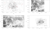 |
Fig. 1. Spatial distribution of GES targets (black dots) and OB stars (red symbols) (upper/left panel), WFI and VPHAS+ sources (upper right and lower left panels, respectively) and X-ray detections (lower right panel). |
2.2. Optical and NIR photometry
Several deep optical and NIR astrometric/photometric catalogues in the region of NGC 6530 are available in the literature:
-
BVI photometry (down to V ∼ 23) obtained from the Wide Field Imager (WFI) at the MPG/ESO 2.2 m telescope within a field of view (FOV) of 34′ × 33′ (Prisinzano et al. 2005). This catalogue includes a total of 53 581 objects, also taking into account the bright sources found by Sung et al. (2000). The spatial distribution of the WFI sources is shown in the upper right panel of Fig. 1.
-
ugriHα VPHAS+ (Drew et al. 2014) photometry described in Kalari et al. (2015). In the region covered by the GES data this catalogue includes 94 826 sources. Their spatial distribution is shown in the lower left panel of Fig. 1.
-
JHK NIR photometry taken from the All-Sky Point Source public catalogue of the 2MASS (Cutri et al. 2003).
-
3.6, 4.5, 5.8, and 8.0 μm bands Spitzer IRAC photometry within a FOV of
 ×
×  , from which 64 Class I/0 and 168 Class II sources have been identified by Kumar & Anandarao (2010).
 -
NIR and mid infrared (MIR) spectral energy distributions (SED) excess sources defined in the MYStIX Probable Complex Members (MPCMs) (Feigelson et al. 2013; Broos et al. 2013). Objects with IR excess were identified by modelling their NIR/MIR SEDs as circumstellar dust in a disc or infalling envelope as done in Povich et al. (2011).
-
parallaxes and proper motions from the Gaia DR2 catalogue (Gaia Collaboration 2016, 2018; Lindegren et al. 2018).
2.3. X-ray data
The NGC 6530 region has been covered at high spatial resolution by two X-ray Chandra ACIS-I observations. The first, indicated as ACIS-I/A, was a 60 ks observation carried out on June 18–19, 2001, and was centred on RA = 18h04m , Dec = −24°21′
 . The X-ray analysis was presented in Damiani et al. (2004). The second observation, indicated as ACIS-I/B, centred on RA = 18h03m
 , Dec = −24°22′
 , was a 172 ks observation, obtained from the combination of three ACIS-I observations of 127, 15, and 30 ks, respectively. The FOVs of the two X-ray observations are drawn in the lower right panel of Fig. 1. The two ACIS-I FOVs are partially overlapping and part of the second observation covers a region outside the WFI FOV.
The two observations were combined and a new list of 1510 X-ray detections was derived following the procedure described in Damiani et al. (2004). The spatial distribution of these objects is shown in the lower right panel of Fig. 1.
3. Cross-correlations among catalogues
In this section we first describe how we performed the cross-correlation between the new X-ray catalogue and the WFI/2MASS optical/NIR catalogue. From this catalogue, we only considered objects observed in the Gaia-ESO survey programme for the present analysis.
The number of X-ray sources falling in the WFI FOV is 1415. The number of optical WFI sources found within the two ACIS-I FOVs is 14 229. To cross-correlate the 1415 X-ray sources with the objects in the optical catalogue, we used the procedure described in Prisinzano et al. (2005) and we considered a variable matching radius that takes the X-ray position error, σX into account. We first used a matching distance d = 1σX and found a systematic shift of (RAWFI-RAX) = − and (DecWFI-DecX) =
  between the optical and X-ray positions of the matched objects. We corrected the X-ray coordinates for this shift and cross-correlated the two lists of coordinates again using a matching distance d = 4σX and a minimum matching distance of
  .
.
With these conditions we have a total of 1178 matches, of which 1043 are X-ray sources with 1 optical counterpart, 52 are X-ray sources with 2 optical counterparts, 6 are X-ray sources with 3 optical counterparts, 2 are X-ray sources with 4 optical counterparts and 1 X-ray source with 5 optical counterparts. Therefore, the total number of X-ray sources with WFI counterpart(s) is 1104 while the number of X-ray sources without an optical counterpart is 311.
We considered all X-ray detections, including the 95 X-ray sources falling outside the WFI FOV, and cross-correlated them with the 2MASS catalogue. Since the X-ray coordinates can be shifted with respect to the 2MASS coordinates, we first cross-correlated the entire list of X-ray sources with the 2MASS All-Sky Point Source Catalog, from which we selected only objects obtained from aperture photometry or profile-fitting (ph_qual flag equal to “AAA” or “BBB” or “CCC” or “DDD”). Using the same procedure adopted for the match with the WFI catalogue, we first corrected for the systematic shift in the X-ray positions (RA2MASS-RAX) =  and (Dec2MASS-DecX) =
  . Using the new coordinates, we obtained a total of 462 2MASS counterparts of 444 X-ray sources. Among these, 53 X-ray sources have 2MASS counterpart(s) but no WFI counterpart.
We are left with a catalogue of 54 110 objects including the 53 581 WFI objects from Prisinzano et al. (2005), 123 optical sources from Sung et al. (2000) without WFI counterparts, and the 406 X-ray sources without optical counterparts; only 53 of these latter objects have a 2MASS counterpart. There are 471 GES targets with X-ray counterparts.
Finally, we crossmatched the catalogue of 2077 objects observed with GES with the lists of NGC 6530 candidate members given by Kumar & Anandarao (2010) and Feigelson et al. (2013) and with the Gaia DR2 catalogue in this region. In conclusion, we found that the list of stars spectroscopically observed with GES includes: i) 1733 objects with WFI-BVI photometry; ii) 1423 objects with VPHAS+ riHα magnitudes (Drew et al. 2014; Kalari et al. 2015); iii) 1976 objects with 2MASS counterparts; iv) 50 (8) sources classified as Class II (Class I/O) YSOs, with Spitzer IRAC magnitudes; v) 139 (23) objects classified as Stage O/I or Stage II/III (ambiguous) in the MYstIX project; and vi) 2013 objects with counterparts in the Gaia DR2 catalogue with proper motions (PM) and parallaxes.
4. Membership strategy
The simultaneous use of spectroscopic data with literature optical and NIR photometry and X-ray data can be exploited to study membership in very young clusters at a very accurate level, allowing us to maximize the number of true positives, i.e. the confirmed members, and minimizing the number of false positives, i.e. the contaminants. This is crucial for selecting a sample as complete as possible, since the combination of the available indicators allows us to reject true negatives (non-members) and to retain as many as possible false negatives, which are genuine members passing some criteria that are negatives for other criteria.
For example, there are strong youth criteria such as high values of EW(Li) or IR excesses and broad Hα emission lines, signatures of circumstellar discs and accretion/outflow, respectively, which are very useful to select confirmed members (true positives). In fact, it is very unlikely that they select contaminants (false positives) since the timescales typical of discs and accretion are relatively low (smaller than few 10 Myr). Nevertheless, there are objects that can be negative for some criteria and positive for others. For example, objects with EW(Li) smaller than the adopted threshold or without IR or Hα line excesses, can be either early type or lithium depleted young stellar objects (YSOs; Palla et al. 2007; Sacco et al. 2007) or even YSOs without circumstellar discs and accretion processes.
Other criteria, such as the X-ray emission from young stars are known to decay on longer timescales, depending on the spectral type (Jeffries et al. 2014; Prisinzano et al. 2016). Therefore, if all X-ray detected objects are considered young stars, they are likely to include a low but not negligible fraction of false positives, since there is a chance to find ∼100–200 Myr old field stars or older close binary stars with X-ray emission, which are unrelated to the young cluster (Wright et al. 2010). Even for X-rays, false negatives can be found, depending on the spectral types or observational limits.
The RV membership criterion, by selecting the stars with RV around the cluster mean RV, allows us to include a large fraction of true positives, but, for this indicator, the chance to include also false positives is not negligible. On the other hand, false negatives that are genuine members with RVs outside the cluster RV range can be found if the objects are binaries or if the RV is not well determined as in case of artefact lines in the spectra with uncorrected sky subtraction due to the strong nebular contribution (see Damiani et al. 2017a). A further kinematic membership criterion is provided by Gaia DR2 PMs and parallaxes, since these allow us to select stars with a common motion that are located at similar distances.
Finally, the γ index defined by Damiani et al. (2014), being an indicator of the stellar gravity, is a very useful criterion to select true negatives. In fact, Damiani et al. (2014) showed that for late spectral type stars, the γ index of giants is significantly larger than that of PMS stars, that is only slightly larger than that of MS stars. For this reason, the γ index can be used to select giants and then to discard them as true negatives from the sample of YSOs.
In order to exploit all available criteria and take into account both their potential and limitations, in this work we adopted the following membership strategy. We first defined as candidate members all the objects that are positives in at least two of the following membership criteria: RV, EW(Li), Hα FWZI, photometric r-Hα colour excesses (Kalari et al. 2015), X-ray detections, NIR/MIR colour excesses, Spitzer IRAC colour excesses (Kumar & Anandarao 2010), and Gaia DR2 PMs and parallaxes. Finally, we discarded all expected true negatives based on the γ index.
With this strategy we are confident of maximizing the number of certain members (true positives) and discarding as many contaminants (false positives) as possible, and not to discard a priori genuine members that are negatives to one or more criteria (false negatives) and reject only non-members (true negatives). In fact, the probability of selecting false positives simultaneously using more than one criterion (even only two) is definitively lower than that of using only one criterion. At the same time, using simultaneously two membership criteria, without a priori discarding (false or true) negatives for all the criteria, allows us to not discard genuine members, leaving us the opportunity to study the global properties of the cluster. In addition, this strategy reduces the bias from the lack of youth or membership indication in one or more criteria due to observational limits. In the following subsections, we detail the selection of the candidate members that includes in this step both true and false positives, for each of the adopted criteria.
4.1. Radial velocities
The first step in selecting candidate cluster members by their RV is to study the RV distribution of a very reliable sample of cluster members (only true positives). This is crucial to derive the shape of the cluster RV distribution and therefore its statistical properties. The sample suitable to model the cluster RV distribution has been chosen from a sample of filtered members where all possible negatives were discarded as described in Randich et al. (2018). The maximum-likelihood technique adopted to model the observed RV distribution has recently been described for other clusters in Randich et al. (2018) and it has been previously adopted for other clusters included in the GES project (Jeffries et al. 2014; Sacco et al. 2015). The technique takes into account the binary contribution (Cottaar et al. 2012) and the uncertainty distribution (Jackson et al. 2015). In addition, to take into account the fraction of contaminants included in the starting samples, the model consists of two Gaussian components: one for the cluster and one broad Gaussian for the background of the contaminating stars. In the case of NGC 6530, the best fitting parameters we found are RVcl = 0.17 km s−1 and σcl = 2.42 km s−1 for the cluster and RVfld = −10.69 km s−1 and σfld = 32.17 km s−1 for the field stars. The fraction of stars belonging to the cluster population is fcl = 0.44. A more detailed study of the kinematics and RV distribution of Lagoon Nebula is presented in Wright et al. (2019).
Based on these results, we consider the RVcl and σcl as representative for the cluster RV distribution and we consider as candidate members, positives with respect to RV criterion, all the objects with RV around RVcl and within 5σcl, corresponding to a probability lower than 0.57 parts per million1 of finding cluster members outside this range. The true probability is larger than this value since the uncertainty distribution has extended tails that are better represented by a Student-s t-distribution than a by normal distribution (Jackson et al. 2015). With this criterion, we selected 893 RV candidate members.
4.2. Lithium equivalent width
Theoretical models predict that stars with ages younger than 10 Myr have cosmic abundances of lithium (Baraffe et al. 1998; Siess et al. 2000). In order to establish a EW(Li) threshold suitable to include a list as complete as possible of members, we considered the EW(Li) distribution as a function of the effective temperatures of the RV candidate members, mostly formed by cluster members. We found that most of the potential members have EW(Li) >200 mÅ for stars with Teff ≲ 5200 K. For stars with Teff ≳ 5200 K, the EW(Li) of possible members is in the range [100–200] mÅ, even though at these temperatures the lithium strength is no longer a sensitive age indicator. As mentioned before, we cannot discard a priori the presence of lithium depleted (or partially depleted) members with Teff ≲ 5200 K, as found in other young star forming regions (Palla et al. 2007; Sacco et al. 2007). Therefore, we adopted a conservative threshold of 100 mÅ, independent of the effective temperature, and defined as EW(Li) candidate members all objects with EW(Li) larger than this value. Using this relatively low threshold, we are aware of the risk of also including false positives, many of which will be discarded with the final selection. On the other hand, we include most of the candidate members with Teff ≳ 5200 K and potential depleted objects. There are 545 observed stars with EW(Li) >100 mÅ.
4.3. Hα line
The Hα line in spectra of young stars is a strong signature of chromospheric activity, producing emission in the core of the line, or of circumstellar accretion and outflow, producing emission of broadened lines due to high velocities of the gas when it impacts the stellar surface (Bonito et al. 2013; Prisinzano et al. 2016). Chromospheric activity can be quantified through the Hα equivalent width (EWHaChr) values from the GES recommended parameters or the αc indices (measuring flux in the line core) defined in Damiani et al. (2014), while accretors can be selected from the Hα 10% width or from the FWZI used for example in Prisinzano et al. (2007) and Bonito et al. (2013). In the case of a young cluster such as NGC 6530, surrounded by an H II region, the Hα line in the observed stellar spectra also includes a significant contribution from the surrounding nebulosity. Because of the complex dynamics of the ionized nebular gas (Damiani et al. 2017b), this contribution cannot be rigorously quantified and subtracted with the traditional technique of the mean sky, i.e. estimated by taking a number of sky spectra from the same region. In fact, sky subtraction can be over or underdone (Bonito et al., in prep.); therefore all measurements involving the peak of the Hα line, such as the Hα 10% or EWs, EWHaChr, and αc indices, are not reliable to quantify the stellar Hα contribution. Nevertheless, while the accretion process implies a significant line broadening, the nebular emission typically onlyaffects the line core. Therefore, spectra of accretors can be distinguished from those of non-accretors with chromospheric activity or sky nebular emission, using the Hα line FWZI, that is the only measurement independent of line peak intensity. We used the GES recommended parameter FWZI and selected as candidate accretors all the objects that, within errors2, have FWZI >4 Å. This threshold has been chosen because the objects with NIR (from JHK or Spitzer IRAC magnitudes) or VPHAS+ r-Hα excesses have FWZI ≳ 5 Å. With this condition, we selected 241 candidate accretors. To this sample we added 31 of the 235 accretors defined in Kalari et al. (2015) using the r-Hα excesses; these are included in the GES sample.
4.4. X-ray and NIR/MIR membership
Among the 2077 stars observed within GES, there are 471 objects also detected in X-rays and 243 objects with IR excesses in JHK colours, according to the extinction-free indices defined in Prisinzano et al. (2007). In addition, we also considered the 50 Class II and 8 Class 0/I stars defined in Kumar & Anandarao (2010) and the 162 YSOs selected in the MPCMs project (Feigelson et al. 2013; Broos et al. 2013), that are included in the GES sample. We considered these samples as candidate cluster members.
4.5. Kinematic membership with Gaia DR2
To define the range of PMs and parallaxes of candidate cluster members, we first considered a fiducial sample of members confirmed by at least three of the membership criteria described in the previous subsections. For this subsample, we computed the median of PMs μα*3 and μδ and parallaxes π that are 1.34 mas yr−1, −2.03 mas yr−1, and 0.74 mas, respectively, and the relative standard deviations that are 1.34 mas yr−1, 0.93 mas yr−1, and 0.45 mas, respectively.
We considered as candidate members those within the two ellipses in the planes μα* versus μδ and μα* versus π, where the semi-minor and semi-major axes were defined by the 1σ values of the fiducial sample of cluster members. With these criteria we selected 516 candidate members from Gaia DR2 data among the 2077 GES targets. Gaia DR2 data together with GES RVs are analysed in Wright et al. (2019).
4.6. Final membership for GES targets
By combining the previous criteria, we selected 661 objects that are included in at least two of the candidate member samples previously defined and have γ indexes smaller than 1.018. This latter condition was applied to reject non-members, for which gravity (inferred from the γ index) was inconsistent with PMS stars. We consider as probable members the 9 objects with Teff > 5200 K for which the EW(Li) is in the range [100, 200] mÅ since in these cases the EW(Li) is not a strong age indicator and therefore for these objects their membership is positive only for one criterion. The remaining 652 objects are classified as confirmed members.
Among the 661 confirmed or probable members, 333 were classified as classical T Tauri stars with excess (CTTSe), including accretors, on the basis of the Hα FWZI or the r-Hα colours, or objects with circumstellar disc, on the basis of NIR excesses. The remaining 328 members were classified as weak T Tauri stars with photospheric emission (WTTSp) including members without evidence of accretion and without evidence of circumstellar disc. Literature and Gaia-ESO survey parameters of the selected cluster members are given in Tables A.1 and A.2. Figure 2 shows the μδ versus μα* and the π versus μα* scatter plots of all objects observed with GES. Stars selected as confirmed or probable members are highlighted with different colours. The RV distribution and EW(Li) as a function of the effective temperature of the 661 objects selected as confirmed or probable members are also shown. There are few objects with proper motions or parallax values outside from the typical cluster values. We checked that most of these are objects with excess noise > 1.0 mas and/or χ2 > 800 (Lindegren et al. 2012) and/or with parallax errors > 0.3, which means they could be binaries or objects for which the Gaia DR2 kinematic parameters are not well determined because of confusion caused by the large stellar density towards NGC 6530.
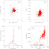 |
Fig. 2. Gaia DR2 proper motion scatter plot (panel a), Gaia DR2 parallaxes vs. μδ (panel b), RV distribution (panel c), and EW(Li) as a function of the effective temperature (panel d) of all GES targets (black symbols). Objects selected as confirmed (probable) cluster members are indicated as red (cyan) dots. The red histogram in panel c is the RV distribution of the confirmed cluster members, while dashed red lines are the limits used for the selection of RV candidate members. |
5. Candidate giants and MS field stars in the GES sample
In combination with the observed colours, GES effective temperatures of field stars can be used to derive the interstellar reddening of these objects and therefore to study the properties of the dust component of the Lagoon Nebula.
The sample of non-members includes both MS stars and giants; the latter are expected to be found mostly at distances significantly larger than the cluster distance, i.e. beyond the Lagoon Nebula, while MS stars are expected to be found both in front of and behind the nebula.
We describe in this section the use of the γ index defined by Damiani et al. (2014) to define candidate giants within the GES sample of cluster non-members. Figure 3 shows the γ index as a function of the effective temperature for all the objects classified as members and non-members. The dashed curve indicates the locus of MS stars from Damiani et al. (2014). Giant stars have lower gravities and therefore γ indices higher than this limit. In addition, red giants are expected to have effective temperatures Teff < 6030 K, based on the Bessell & Brett (1988) relations. Very hot giants are very uncommon. Based on these considerations, we selected as candidate giants all the objects with γ indices higher than the horizontal limits shown in Fig. 3. The limits are temperature dependent to ensure the selection of objects with γ indices larger than the MS locus. In particular, we adopted a lower threshold (γ > 0.99) for T < 5300 K, where the γ index is more sensitive to the gravity and the separation between MS stars and giants is larger while, for 5300 < T/K < 6030, we used the limit γ > 1.01. We note that for 4700 < T/[K]< 5300 and γ > 0.99, many candidate giants have γ values similar to those of objects selected as young cluster members. This occurs since as predicted by theoretical models in this range of effective temperatures the ranges of gravities of giants and PMS stars younger than few million years overlap (see Fig. 4 of Damiani et al. 2014). We also included in the giant sample the few objects with T > 6030 K and γ > 1.03. This sample includes 237 + 33 + 11 = 281 candidate giants that are shown as green squares in the Fig. 3.
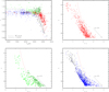 |
Fig. 3. γ index as a function of effective temperature (upper/left panel) and observed V vs. V-I diagrams of the GES targets selected as cluster members (red bullets), candidate giants (green squares), RC giants (magenta plus symbols), foreground (black bullets), and background (blue bullets) MS stars. The horizontal solid segments and the dashed line in the upper left panel indicate the limits used to select giants and the MS locus, respectively. The red solid line in the other panels is the 0.1 Myr PISA isochrone described in the text. |
The CMDs of cluster members and candidate giants are shown in Fig. 3 (upper right and lower left panels, respectively). Most of the selected giants fall outside of the expected PMS region in the V versus V − I diagram distributed along the reddening vector direction. As already noted in Prisinzano et al. (2005), these objects are dominated by very distant and reddened red clump (RC) giants (Girardi 1999). Among the sample of 281 giants, we selected the subsample of RC giants, as the objects with V − I colours redder than the 0.1 Myr isochrone computed using the updated version of the PISA stellar evolution code (see e.g. Randich et al. 2018; Tognelli et al. 2018). The isochrone has been positioned at the cluster distance of 1250 pc (Prisinzano et al. 2005), assuming a mean reddening E(B − V) = 0.3 and the reddening law of RV = AV/E(B − V) = 5.0. With this condition, we find that 117 of the selected objects are RC giants.
While we are confident that these 117 are confirmed giants, the remaining sample of 164 candidate giants could be contaminated by MS stars, since for early type stars, the γ index is not very sensitive in separating objects with different luminosity classes. We consider all the remaining GES objects as the field MS stars, i.e. those that are neither classified as cluster members nor giants. The CMD of MS stars is shown in Fig. 3 (lower right panel).
6. Interstellar reddening
To convert GES effective temperatures and surface gravity data to colours, we computed transformations using the synthetic spectra library by Castelli & Kurucz (2003) for Teff > 6500 K and the Allard et al. (2011) spectra for Teff < 6500 K, integrated over the adopted filter response. For giants, we used the Bessell & Brett (1988) intrinsic colour transformations.
To derive the interstellar reddening, we used the V − I colours since the V and I magnitudes are those for which additional non-photospheric contributions, from dust in the circumstellar disc or blue excesses from accretion, are negligible.
We only used optical WFI photometry rather than the VPHAS+ photometry since the members (probable and confirmed) for which both effective temperatures and the WFI V − I (VPHAS+ r − i) colours are available are in total 395 (364); there are 337 common objects within the two samples. In addition, the anomalous reddening law adopted in this work for the cluster is defined in the Johnson-Cousin system.
Figure 4 shows E(V − I) as a function of the effective temperatures for the samples selected before, i.e. for cluster members, MS field stars, and giants. As expected, most of the cluster members (upper panel) share a similar reddening.
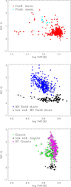 |
Fig. 4. Interstellar reddening E(V − I) vs. effective temperature for cluster members, MS, and giant field stars. |
In particular, there are 361 confirmed cluster members with E(V − I) < 1. For this sample, the mean of the E(V − I) values is ⟨E(V − I)⟩ = 0.50 and the standard deviation is 0.17, and ⟨E(B − V)⟩ = 0.27 and the standard deviation is 0.17. The ⟨E(B − V)⟩ we found is in good agreement with that given in the literature (E(B − V) = 0.30 − 0.37; see e.g. van den Ancker et al. 1997; Sung et al. 2000; Tothill et al. 2008).
There are 26 members with E(V − I) > 1. Cluster membership is confirmed by more than two methods for 17 of these and by two methods (RV and X-rays or RV and CTTS signatures or, in one case, strong EW(Li) and CTTS signature) for 9 of these. We consider these objects as very reddened confirmed cluster members since there is no reason to discard them as members only because of their higher reddening. Their properties are discussed in the next sections. In addition, there are further 8 objects, classified as probable cluster members, with E(V − I)> 1.
The E(V − I) distribution of the sample of MS field stars is also shown Fig. 4 (middle panel). Even in this case, there is a sample of very low reddening MS stars (see also Fig. 3). Those with E(V − I) < 0.5 have a mean ⟨E(V − I)⟩ = 0.31(⟨E(B − V)⟩ = 0.22) and a standard deviation of 0.13 (0.14). These values, distributed within a very narrow reddening range, are slightly smaller than those found for the cluster, and this suggests, as expected, they are MS stars located in front of the Lagoon Nebula. In contrast, in the sample of highly reddened MS stars, reddening values are spread over a larger range, 0.8 ≲ E(V − I)≲2.5, with a clear gap in the E(V − I) distribution corresponding to members. This suggests they are located at a larger distance, and therefore, beyond the Lagoon Nebula.
We find a similar result for the sample of objects classified in this work as giants (lower panel in Fig. 4). There are few low reddening candidate giants with E(V − I) < 0.2, expected to be nearby objects, while most other giants suffer from large reddening. This latter sample includes all the RC giants selected above with a trend in the E(V − I) values, where hotter RC giants are more reddened than cooler giants. Again, we explain this trend as a distance effect, the hotter giants being also brighter, and therefore visible at a larger distance. A very flat distribution of E(V − I) is instead found for the non-RC giants with E(V − I)∼1.1; these are likely located at a mean distance smaller than the RC giant distances, not far beyond the Lagoon Nebula.
The correlation between the distance of the different samples with their reddening is confirmed by the Gaia DR2 data. Figure 5 shows the distance derived from the Gaia DR2 parallax for the same samples shown in Fig. 4 as function of the effective temperatures. For these plots, we selected only objects with relative errors in parallax < 20%.
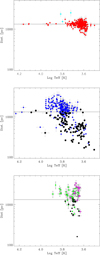 |
Fig. 5. Distances vs. effective temperatures for cluster members, MS, and giant field stars derived using Gaia DR2 data. Symbol colours are indicated as in Fig. 4. The horizontal solid line indicates the cluster distance. |
Cluster members are distributed around a mean distance of  pc computed from the weighted mean parallax equal to 0.7573 ± 0.0403 mas. This value was obtained using the fiducial sample including all the objects that are members for at least three criteria. The error on the parallax was computed as the error on the mean. To this, we added the systematic error equal to 0.04 mas (Lindegren et al. 2016) estimated for Gaia DR2 parallaxes. The value of the cluster distance we found is only slightly higher, but in agreement within the errors with the value of 1250 pc derived in Prisinzano et al. (2005).
Main sequence and giants affected by low reddening (E(V − I)≲0.5) are in front of the cluster, i.e. foreground field stars. The foreground MS stars show quite a linear trend with the distances that increase towards hotter stars (i.e. the most luminous stars).
In contrast, MS and giants affected by high reddening (E(V − I)≳1) are found behind the nebula and the cluster. This confirms that the reddening is strongly correlated with the distance and that the reddening gap both for MS stars and giants is due to the dust in the Lagoon Nebula.
7. Reddening law
In a paper dedicated to the study of the interstellar extinction and its variations with wavelength, Cardelli et al. (1989) computed for the star Herschel 36 an extinction law RV = AV/E(B − V) = 5.3, i.e. a peculiar value that is higher than the standard value, RV = 3.1, usually adopted for the Galaxy. Since the work of Walker (1957), who first suggested an abnormal extinction law, several authors have confirmed this result, but at the same time, the analysis of other observations has favoured a standard reddening law in the cluster NGC 6530 (see Tothill et al. 2008, for a review). The dataset used in this work, including both photometric and spectroscopic information, can be exploited in several ways to investigate the reddening law in this region.
As a first step, we considered the sample of confirmed cluster members, classified in Sect. 4.6, as WTTSp stars. This choice was made to ensure that the observed colours only depend on interstellar reddening (and Teff). In fact, peculiar objects such as the CTTSe might have colours that include other contributions due to dust or gas in their circumstellar disc.
For the WTTSp cluster members, we compared several observed colour-colour diagrams with the expected unreddened intrinsic colours, as shown in Fig. 6. By shifting this locus along the reddening vector for a suitable reddening law, a reasonable match between the intrinsic reddened locus and the observations should be found.
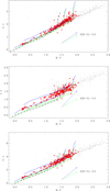 |
Fig. 6. Colour-colour diagrams of the GES targets (black dots) and WTTSp cluster members (red points) for three different sets of colour combinations. The dashed black line is the theoretical colour-colour locus adopted in this work (see Sect. 6). Green and blue solid lines are the same locus reddened by E(B − V) = 0.2 and 0.5 assuming RV = 3.1 and RV = 5.0, respectively. |
Since most WTTSp in our sample have E(B − V) values between 0.2 and 0.5, we shifted the adopted intrinsic relation assuming these two values, with the aim of matching the bulk of the observed colours. As it is known, in the colour-colour diagrams shown in Fig. 6, the intrinsic colour-colour locus is degenerate with respect to the reddening direction, except in the range of the M-type stars (Damiani 2018); in this range the intrinsic locus bends towards a different direction and has a slower variation in the bluer B − V colours than in the redder colours.
We find that assuming the reddening relations given in Fiorucci & Munari (2003) for RV = 3.1, the two shifted loci (green lines) do not satisfactorily describe the data, since only the M-type part of the intrinsic colour relation can match our data. In contrast, assuming the anomalous wavelength reddening relations, RV = 5.0 by Fiorucci & Munari (2003), the reddened loci (blue lines) can match our data along the entire range of spectral types. We consider this as an evidence that the members of NGC 6530 obey the abnormal reddening law, rather than the standard law.
A further way to investigate the reddening law valid for the cluster members is to compare the individual reddening ratios, derived spectroscopically as described in the previous section, for several photometric bands and compare these with the analogous ratios expected for RV = 3.1 and RV = 5.0. Also in this case, we used the sample of WTTSp with Teff > 4000 K. The individual reddening ratios as a function of the effective temperatures are shown in Fig. 7. The observed spread is dominated by the individual errors rather than the intrinsic dispersion. Nevertheless, despite the quite large dispersion the mean values of the ratios in the given photometric colour combinations are in agreement, within the errors, with the abnormal reddening law RV = 5.0 rather than with the standard law, as shown in the lower right panel of Fig. 7.
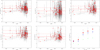 |
Fig. 7. First five panels: ratios of individual reddenings in several combinations of colours as a function of the effective temperatures for all GES targets (small dots) and for WTTSp cluster members with Teff > 4000 K (red points). Lower right panel: mean ratios of reddening values for the WTTSp cluster members in several colours (red circles), compared with the expected analogous values given for RV = 3.1 (green plus symbols) and RV = 5.0 (blue squares) based on the Fiorucci & Munari (2003) relations. |
Our data offer a further opportunity to investigate the reddening law in the region around NGC 6530 by also considering the sample of giants. As described in Sect. 5, the sample of GES targets includes a subsample of RC giants, i.e. stars in the core helium-burning phase (Girardi 1999). We expect most of these belong to the bulge and are located within a relatively small range of distances with respect to the other giants. These objects have similar intrinsic astrophysical properties, such as temperature and luminosity, at a given metallicity and age. These properties have been exploited in the past to derive reddening maps in several regions and also to derive the reddening law, as done in De Marchi et al. (2014, 2016) for the 30 Doradus Nebula. In fact, assuming similar magnitudes and colours, their distribution in the CMD is a signature of the amount of interstellar reddening affecting them, while the slope of their distribution corresponds to the ratio R between absolute and selective extinction in the specific colour.
As in De Marchi et al. (2014, 2016), we performed a linear fit in the CMD to the RC giants. We note that De Marchi et al. (2014, 2016) identified a compact and well-defined locus of the RC giants in the 30 Doradus CMD, which shows a larger spread in our CMD, due to the larger apparent size of the bulge compared to the LMC. However the slope of their distribution can be used to estimate the reddening law in our case as well. The resulting slopes are overplotted in the CMDs of Fig. 8, where the comparison with the Fiorucci & Munari (2003) relations given for RV = 3.1 and 5.0 is also shown. The uncertainty related to the range of distances in the bulge cannot significantly affect our results.
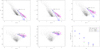 |
Fig. 8. First five panels: CMD of all GES targets (small black dots) of the BVIJH magnitudes as a function of B − V. RC giants are indicated with magenta plus symbols. The black solid line indicates the slope obtained by the fit; the green and blue arrows indicate the reddening vectors corresponding to the standard and abnormal reddening laws, respectively. The lower right panel shows a comparison of the fitted slopes for RV giants in various photometric bands with the literature reddening laws. |
We performed the analogous fit on the colour-colour diagrams and we obtained the results shown in Fig. 9. We note that the colour-colour diagram slope fitting is independent of the distance and therefore the results are more robust than those obtained from the CMD. However, the fitting results, both in the CMD and the colour-colour diagram suggest that unlike the cluster members, RC giants follow a standard rather than an abnormal reddening law.
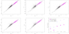 |
Fig. 9. First five panels: colour-colour diagrams of all GES targets. The RC giants are indicated with magenta plus symbols. The black solid line indicates the slope obtained from the fit. Lower right panel: a comparison of the obtained slopes with the literature reddening laws. |
As we have done for the cluster members, we also used the individual reddening derived spectroscopically and computed the ratios between the reddening in several colours and E(B − V). In this case, the statistical errors on the effective temperatures and possible systematic errors on reddening from the sample selection (mis-classification of the luminosity class) or to the colour-temperature relations, contribute to enhance the observed spread in the reddening ratios. In order to reduce such dispersion, we selected only the RC giants with errors in reddening ratios smaller than 0.4 mag. Figure 10 shows such ratios as a function of the effective temperatures. The comparison of the mean ratios with the analogous ratios found from the CMD and those with the values given in Fiorucci & Munari (2003) are also shown.
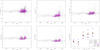 |
Fig. 10. First five panels: reddening ratios in several colours over E(B − V) for all GES targets. The RC giants are indicated with magenta plus symbols. The black (dashed) solid line is the mean (standard deviation) obtained for RC giants. Lower right panel: comparison of the slopes obtained from the photometric and spectroscopic data with those given in the literature for various reddening laws. |
The spectroscopic data suggest that the reddening law of the RC giants is marginally consistent with the standard reddening law, unlike the photometric data. Instead, spectroscopic results suggest an intermediate reddening law that is compatible with an intermediate RV value, like RV = 4.0. The background giants should experience a combination of extinction due to both the large dust grains in the Lagoon Nebula (with an abnormal reddening law) and the background interstellar extinction (with a standard reddening law). For this reason, we expect the reddening law measured for the background stars to be somewhere between the RV = 3.1 and RV = 5.0 reddening laws, as suggested by our spectroscopic results.
In conclusion we find that while an anomalous reddening law is more appropriate to derive the stellar absorption towards cluster members, around background objects such as RC giants the reddening law is, instead, between standard and abnormal.
The indication of an anomalous reddening law around cluster members, obtained in two independent ways, supports the hypothesis of the prevalence of large dust grains with respect to small grains. This can be explained with the evaporation of small grains by the radiation of O-B type stars, or with the grain growth in the circumstellar disc (Tothill et al. 2008), in agreement with recent planet formation theories (Mordasini et al. 2012; Gonzalez et al. 2017).
8. Spatial distributions and nebula structure
The open cluster NGC 6530 and the surrounding nebula have been described in the literature as having a complex spatial structure (e.g. Tothill et al. 2008). As already mentioned in the previous sections, our data provides us with fundamental stellar parameters, such as effective temperatures, gravities, and reddenings, not only for the cluster population but also for the field stars falling in the same field. In the following we show how these parameters can be used to derive suggestions of the thickness of the nebula.
Individual reddenings found for the various populations of stars also give us indications about their expected distance and relative position, since our ability to reach objects at very large distance is strongly related to the transparency of the material between us and them. Therefore, the properties of these objects can be used as tracers of the interstellar material.
In this section we study the spatial distribution of the three main populations selected in this work, i.e. cluster members, MS, and giant field stars, with the aim of connecting their location on the sky with the properties of the nebula surrounding the cluster NGC 6530.
Figure 11 shows the spatial distribution of cluster members, MS, and field stars for which the interstellar reddenings have been derived, i.e. the GES targets with optical WFI photometry (Prisinzano et al. 2005). The comparison shows that the cluster is dominated by objects with reddening significantly different from that affecting MS stars and giants. Cluster members are mainly concentrated in the region delimited by the subclumps found by Kuhn et al. (2014), where most of the OB-type stars are found, while the populations of MS and giants are more randomly distributed.
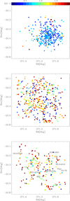 |
Fig. 11. Spatial distributions of cluster members (upper panel), candidate MS stars (middle panel), and giant stars (lower panel), for which the reddening has been derived. Symbol colours are drawn as function of E(V − I) as defined in the colour bar. For a better readability, the positions of massive stars are shown in the lower panel only. |
The spatial distribution of MS stars and giants form a patchy pattern with subregions completely devoid of stars. We note, however, that the few MS field stars affected by very small reddening, expected to be foreground objects, are quite uniformly distributed on the field, while the peculiar pattern is mainly drawn by the stars affected by higher reddening, expected to be located at distances similar to the cluster or further away. We interpret this latter peculiar spatial distribution as evidence of the non-uniform transparency of the surrounding Lagoon Nebula, connected to its thickness.
In particular, there are two regions, roughly centred at (271.15, −24.27) and (271.07, −24.5), which are almost empty of background stars. We suggest these are the darkest and thickest parts of the nebula. where background stars are too extincted to be detected with our observational limits. In contrast, most of the reddened field stars are found outside these regions, which correspond to less extincted areas of the nebula, where the thickness is instead lower.
The spatial distribution of giants is characterized by a lower stellar density but a pattern similar to that found for MS background stars since the subregions devoid of (filled with) MS stars correspond to those devoid of (filled with) giants.
This confirms our hypothesis concerning the nebula structure. In fact, RC giants are very distant objects and are expected to be homogeneously distributed across the sky since the cluster NGC 6530 is located close to the direction of the Galactic centre. Our results indicate for increasing reddening values for RC giants (with respect to cluster members); this fact is consistent with the hypothesis of very distant objects with an apparent inhomogeneous spatial distribution, which is correlated with the interstellar material transparency. This confirms that the regions devoid of giants are likely very opaque areas where the Lagoon Nebula dust prevents detection of objects behind it.
The anti-correlated spatial distributions of cluster members and field stars, and the consequent evidence of a different transparency of the nebula around these different stellar populations, is consistent with the various reddening laws found in Sect. 7 for cluster members and giant stars. In fact, the reddening law is strongly dependent on the grain size distribution of the interstellar material (Mathis & Wallenhorst 1981). In the direction of the cluster centre, small dust grains of the background interstellar medium are likely not detected because of the thickness of the nebula. In addition, owing to the evaporation of small grains by radiation from massive stars and the presence of a large number of YSOs with circumstellar discs, the grain size distribution of the nebula is expected to be dominated by larger-than-average grains. In contrast, in the regions in which the nebula is not opaque, the reddening is dominated by the interstellar material properties up to very large distances, and therefore by a standard reddening law.
9. Age and gravity spread
As shown in Sect. 7, the reddening law appropriate to NGC 6530 cluster members is RV = 5.0. Using this relation and the individual reddening values E(V − I) obtained as described in Sect. 6, we derived individual absorption values AV for the samples including the 147 WTTSp members and the 240 CTTSe members with WFI V and I photometry. For these samples we also computed stellar luminosities, masses, and ages using the recent PISA stellar evolutionary models for solar metallicity and the cluster distance 1320 pc that is the weighted mean distance found in Sect. 6.
Figure 12 shows the intrinsic V0 versus (V − I)0 and the HR diagrams for the 147 WTTSp and the 240 CTTSe members compared with the adopted tracks and isochrones. Isochronal ages were assigned by the bilinear interpolation of the adopted isochrones to the position of cluster members in the V0 versus (V − I)0 diagram. Age values are given in Table A.2.
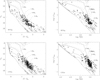 |
Fig. 12. V0 vs. (V − I)0 (left panels) and the HR (right panels) diagrams for members classified as WTTSp (upper panels) and CTTSe (lower panels). The dashed and solid lines indicate the PISA evolutionary tracks and isochrones at masses and ages indicated in each panel and at the cluster distance. |
Figure 13 shows the histograms of isochronal stellar ages derived for all members, WTTSp and CTTSe. The distributions are approximately log-normal, and therefore we quote means and dispersions in dex rather than linear units.
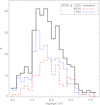 |
Fig. 13. Isochronal age distribution of all members, WTTSp, and CTTSe drawn as solid black, dashed red, and dotted blue histograms, respectively. |
We find that the hotter stars are, or look, older than cool stars, which is a common problem (yet unsolved) when looking at star forming regions. For this reason we did not include hotter stars in the calculation of the statistical parameters of the sample. Cluster members with Teff < 5500 K have masses in the range [0.24–2.80] M⊙ and ages between 0.1 and 5 Myr. The mean log age for all members is 5.84 (units of years) with a dispersion of 0.36 dex. If we consider WTTSp and CTTSe separately, the mean log age is 5.92 for WTTSp and 5.81 for CTTSe with dispersions of 0.35 and 0.37 dex, respectively. The two latter distributions are marginally different as confirmed by the Kolmogorow-Smirnov test (KS test), which returns a probability of 0.016 that the two distributions come from the same parent sample. As expected, the number of CTTSe with younger ages is larger than that of WTTSp but the two dispersions are very similar.
To establish if the age dispersion is significant or dominated by the total errors on stellar ages, we quantified the errors on the isochronal stellar ages by performing Monte Carlo simulations, as described in the following section.
9.1. Error estimates: Monte Carlo simulations
Errors on ages depend on several observational uncertainties that affect our ability to accurately position each star in the V0 versus (V − I)0 diagram, and also on the stellar variability that causes the stars move across the diagram. In addition, they depend on the model accuracy.
Errors on (V − I)0 depend on the errors in the spectroscopic effective temperature through the colour-Teff relation adopted in our models. We note that the σ(Teff) values adopted in this work were obtained by considering the statistical errors in Teff released by the Gaia-ESO survey, and the systematic errors due to the calibrations, given in Damiani et al. (2014). These latter errors amount to 109, 73, and 50 K for stars with Teff > 5500 K, 4300 < Teff/[K]< 5500, and Teff < 4300 K, respectively.
Error bars of V0 depend on the errors in the observed magnitude V and on the error in the absorption AV. This latter is derived from E(V − I), and therefore depends on the reddening law, the errors in the observed colour V − I, and the errors on (V − I)0.
Global uncertainties on V and V − I include the photometric errors and the effects of photometric variability, in case of stars with variable extinction, accretion bursts, and cool or hot spots (e.g., Gullbring et al. 1998; Baraffe et al. 2009; Cody et al. 2014; Stauffer et al. 2016). All these kinds of variability are expected to affect our ability to derive stellar ages for CTTSe, while stellar ages of WTTSp can be affected only by variability due to cool spots. Nevertheless, the presence of a comparable dispersion in the stellar age distributions of both WTTSp and CTTSe suggests that the observed spread is not mainly determined by photometric variability due to accretion, hot spots, or scattering from reflection nebulae (e.g. Grosso et al. 2003; Luhman et al. 2007). To evaluate the uncertainty due to photometric variability, we used the results by Henderson & Stassun (2012), who found 0.02 ≤ ΔI ≤ 0.2, and we estimated the variability in the V band, using the dI/dV values found by Herbst et al. (1994) for a sample of WTTSp.
For each star, we generated three sets of 1000 values, normally distributed, with dispersions equal to the errors in Teff, V and I of that star. We computed a further normal distribution of 1000 ΔI values with mean ⟨ΔI⟩ = 0.11 and σ(ΔI) = 0.03, which roughly corresponds to a distribution of values between 0.02 and 0.2, as found in Henderson & Stassun (2012) and finally we computed a normal distribution of 1000 dI/dV values with mean ⟨dI/dV⟩ = 0.67 and σ(dI/dV) = 0.13; these latter parameters were derived from the Herbst et al. (1994) values.
We added these five sets of random errors to the observed values V0 and (V − I)0 and then computed 1000 values of stellar ages for each star. The statistical error of the age of each star is the standard deviation of these 1000 values. The typical logarithmic standard deviation (mean value) that we found is 0.09 dex, which we assume as representative mean statistical uncertainty in the isochronal ages.
In our simulations we did not take into account the error on the cluster distance used to locate the isochrones in the V0 versus (V − I)0. At the distance of NGC 6530, this systematic uncertainty affects the position of the isochrones only in the vertical direction of the diagram V0 versus (V − I)0 and would imply the same and constant systematic error on all stellar ages, affecting the accuracy but not the precision, and hence the dispersion in which we are interested.
We did not consider the uncertainty introduced by the adopted models because Reggiani et al. (2011) showed that by adopting three different sets of isochrones, even though the amount of the age spread is slightly model dependent, it is significantly large, regardless of which family of models is adopted.
Finally, our calculation does not include the contribution by unresolved binary companions, since this is not a random error but a systematic bias towards higher luminosities (L), and therefore younger ages. The additional contribution to the luminosity of a single star due to a companion can be described using the Δ log L distribution given in Hartmann (2001), ranging from 0.05 (for the minimum mass companion) to 0.3 (for the equal mass companion).
To estimate the uncertainty due to unresolved binaries, we performed a Monte Carlo simulation by generating a distribution of 1000 Δ log L values between 0.05 and 0.3 as in Hartmann (2001). Then, we generated a coeval sample of 1 Myr old artificial stars with (V − I)0 equal to those of our members and V magnitudes from the 1 Myr isochrone.
To the V magnitude of each artificial star, we added the dV values consistent with the Δ log L binary distribution and computed the corresponding stellar ages. As for the statistical error, we computed the standard deviation of the isochronal ages and found that the typical uncertainty due to unresolved binaries is 0.10 dex with a shift Δ log t = −0.21 dex with respect to the starting stellar age of 1 Myr, in agreement with the results found in Hartmann (2001).
By combining the statistical age error equal to 0.09 dex derived above and the systematic age spread equal to 0.10 dex due to unresolved binaries, we found that the typical total uncertainty in the isochronal ages is 0.13 dex; this value is significantly lower than the observed spread equal to 0.36 dex.
We conclude that observed age dispersion, obtained by considering all members and the WTTSp and CTTSe samples separately, cannot be accounted for by observational uncertainties and is evidence of a small but real age spread. This would imply that star formation in NGC 6530 occurred within few million years, in agreement with what was found also in other star formation rates, such as the Orion Nebula Cluster (e.g. Reggiani et al. 2011) and NGC 2264 (Venuti et al. 2018).
9.2. Gravity spread
To evaluate if the observed age spread is supported by otherobservational evidences, we used a further indicator, i.e. the gravity-sensitive γ index; this indicator changes with stellar ages (Damiani et al. 2014), especially for very young stars. In fact, the aforementioned authors found that the gravity of intermediate and low mass stars for the Chamaeleon I (1–3 Myr) cluster, is lower than that obtained for the γ Vel cluster (5–10 Myr). As a consequence the γ index decreases with ages down to the typical values of MS stars. This suggests that a given age spread should correspond to an analogous gravity spread.
In Damiani et al. (2014) it has been shown that for intermediate and low mass stars, the γ index depends on the effective temperature in the sense that it decreases at lower temperatures. This implies that the sensitivity of the γ index to the stellar gravity (and therefore to age) increases towards later spectral types.
To understand if the observed age spread in NGC 6530 corresponds to a gravity spread, we compared the γ index of cluster members with the γ index typical of MS stars. We performed the comparison by considering CTTSe and WTTSp in two different age ranges by splitting the objects with ages younger and older than 1 Myr, as shown in Fig. 14. We note that we considered only the unbiased sample of members with rotational velocity v sin i <50 km s−1, γ < 1.01 and 3800 < Teff/[K]< 5000.
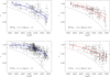 |
Fig. 14. γ index as a function of Teff for WTTSp (upper panels) and CTTSe (lower panels) cluster members split into two different age ranges. The solid lines indicate the best fits obtained from a second order polynomial fit of the data while the dashed line indicates the reference locus of MS stars obtained in Damiani et al. (2014). The dotted lines indicate the polynomial fit at 3σ. |
To avoid possible covariance effects from the dependence on effective temperatures of both the γ index and stellar ages, we performed this test using the stellar ages obtained from the observed V and I magnitudes, which are corrected using the median reddening E(V − I) = 0.5 and are derived from Fig. 4, rather than the individual stellar reddenings, which strongly depend on spectroscopic temperatures. In this way, stellar ages depend only on photometry while the γ indices depend only on spectroscopy and thus the two sets of parameters are fully statistically independent. This choice implies the usage of less certain stellar ages but ensures the robustness of the results.
For each sample, we performed a second order polynomial fit using the ROBUST_POLY_FIT idl routine and compared it with the MS reference locus γMS(Teff) obtained using the γMS(τ) and the τ index versus Teff calibration given in Damiani et al. (2014) for MS stars.
For each sample, we computed the Δγ, defined as the difference between the best fit obtained from our data and the reference locus of the MS stars, as shown in Fig. 15 as a function of Teff. In spite of the large uncertainties affecting the best-fit derivation, the resulting Δγ of the youngest CTTSe is significantly larger than those found for oldest CTTSe. Such difference is not found for WTTSp. All WTTSp, independent of their age, show a Δγ consistent with the oldest CTTSe.
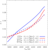 |
Fig. 15. Δγ of CTTSe and WTTSp (solid and dashed lines, respectively) as a function of Teff obtained from the difference between the best fit of the youngest and oldest stars (blue and red lines, respectively) and the reference MS locus. |
To test if the youngest and the oldest CTTSe (116 and 48 objects, respectively) are really two different populations, we performed a KS-test and found a probability of 3.5e–5 that they are taken from the same parent population. In contrast, the probability that the youngest and oldest WTTSp (44 and 38 objects, respectively) are two different populations is 0.77, suggesting that the latter belong to the same population.
The result on CTTSe (the majority of our sample) supports the previous conclusion that the observed age spread is real and it correlates with the gravity spread, as expected.
We note that the observed gravity spread is obtained also assuming stellar ages derived using spectroscopic effective temperatures but, for the reasons discussed above, it is less robust than that shown in Fig. 14.
10. Discussion
Figures 16 and 17 show the spatial distribution of cluster members classified, respectively, as WTTSp and CTTSe, split into the two age ranges used in the previous section and as a function of the proper motion in right ascension μα.
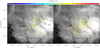 |
Fig. 16. Spatial distributions of WTTSp cluster members split into two different age bins, superimposed on a VPHAS+ Hα image (Drew et al. 2014). The colour codes indicate the Gaia DR2 proper motions in the right ascension. |
 |
Fig. 17. Spatial distributions of CTTSe cluster members split into two different age bins, superimposed on a VPHAS+ Hα image (Drew et al. 2014). The colour codes indicate the Gaia DR2 proper motions in the right ascension. |
These distributions indicate that the WTTSp are sparsely distributed but few of them fall in the region where the youngest CTTSe are found, i.e. around 9 Sgr and Her 36, and along the S-E bright rim to the south of the cluster centre. Even the CTTSe older than 1 Myr in age do not show strong evidence of clustering while the CTTSe formed in the last 1 Myr show a pattern with two radial concentrations. The most populated one is located around the compact core of the cluster NGC 6530, while the second group is in the 9Sgr/Her36 region. In addition, there is a group of CTTSe members formed in the last 1 Myr, which follows the bow-shape structure connecting the Her 36 region with M8E-IR and HD 165052 through the bright Hα rim. The CTTSe of the latter group and those found around 9 Sgr have proper motions μα slightly larger than those of the other members, which agrees with Damiani et al. (2019) and Wright et al. (2019). This is evidence that these latter objects move with a slightly different motion with respect to the other members.
Our findings on the spatial distribution and previous results are used to evaluate two different scenarios. The first scenario is based on the assumption that our stellar age uncertainties are underestimated and that there is not age spread, i.e. all members formed in the same star formation event. According to this scenario, the γ spread found in CTTSe could still be interpreted as a spread in gravity and hence in radius. As is known, low gravity stars in the PMS phase appear more luminous than other stars of the same mass since, as predicted by theoretical models, they descend almost vertically with time along the tracks. These low-gravity objects, for some intrinsic reason, such as episodic accretion, magnetic fields, and starspots, descend along the tracks more slowly with respect to high-gravity stars of the same age and therefore we underestimate their ages, and we misinterpret a luminosity spread as an age spread (e.g. Baraffe et al. 2015). However, we observe that these objects show a very peculiar spatial pattern with respect to the high-gravity CTTSe stars that, in contrast, are sparsely distributed. In addition, the subsample of stars along the S-E bright rim and those around 9 Sgr can be kinematically distinguished from the stars concentrated around the cluster centre. If we assume that the gravity spread is due to an intrinsic property of the star (e.g. episodic accretion, magnetic fields, or starspots), there is no reason for which it should be connected to the spatial regions or to the kinematics of these stars.
An alternative more convincing scenario is that that star formation occurred within few million years but not within a single burst. In this scenario, the gamma spread in the HR diagram is evidence of gravity (and radius) spread due to different stellar contraction stages, i.e. an intrinsic age spread. The youth of these members is supported by their spatial distribution around the cluster centre, where several authors have suggested ongoing star formation. In fact, this region corresponds to the CO bright spot found by Lada et al. (1976) that is receding from us with a heliocentric RV (∼6 km s−1). The CO gas moves away from the cluster centre since its RV is significantly redshifted with respect to the cluster RVcl = 0.17 km s−1. This suggests that very recent star formation events are expected there due to enhanced compression of the gas.
The second group of youngest members is distributed along the bright rim to the south of the cluster centre where CO and dust maps clearly show the presence of a dense molecular cloud. The arch along which the youngest stars are distributed starts from the binary star HD 165052 (O6.5 V + O7.5 V Arias et al. 2002) and ends near the south edge of the Great Rift, i.e. the dark lane that splits the optical nebula. Finally, the remaining youngest stars are found around 9 Sgr, the ionizing star in the Hourglass Nebula, the compact and dense H II region also powered by the O7 star Herschel 36.
A further clue supporting the latter scenario is the different kinematics of the stars in the S-E bright rim and around 9 Sgr with respect to that of stars in the cluster centre. This can be interpreted as evidence of two different star formation events that are pushed and likely triggered by two different ionizing fronts giving origin in the last 1 Myr to different morphology subclusterings: one circularly concentrated (in the cluster centre) and one elongated, following the filamentary morphology of the CO submillimetre arch. This scenario has been already invoked in the past in the literature (see Tothill et al. 2008, for a review).
Our conclusion confirms the Damiani et al. (2014) finding that the γ index undergoes sensitive changes in the first million years for low mass stars with Teff ≲ 5000 K. This is in agreement with the expected increase of gravity during the PMS contraction.
11. Summary and conclusions
Spectroscopic GES parameters cross-correlated with literature data allowed us to identify 652 confirmed members. These include 333 sources with signatures of accretion or circumstellar discs. For the sample of non-members, we used the gravity-sensitive γ index to distinguish the populations of dwarfs and giants. The derived interstellar reddening obtained from spectroscopic effective temperatures, fit in a coherent picture with the inferred luminosity class of the observed objects. In fact, most of the giant stars are also the more reddened sources since they are mainly located behind the nebula, as expected. The foreground stars are mainly MS stars with spectral types earlier than those of giants. Gaia DR2 parallaxes confirm that giants are located behind the nebula while late type (early) MS stars are mainly located in front of (behind) the nebula.
In agreement with previous results from literature, the mean reddening affecting the NGC 6530 cluster members is relatively low and this confirms that the cluster is in front of the surrounding nebula. There are, however, a few members affected by large reddening, that, in contrast, are embedded in the dust of the Lagoon Nebula.
Photometric diagrams and spectroscopic reddening ratios in different bands allowed us to confirm in two independent ways that the reddening law suitable for cluster members is the non-standard RV = 5.0. The result holds only for cluster members and it is likely driven by the complex dust structures around the cluster members. The analogous analysis performed for the background giants located behind the nebula shows that these, in contrast, obey a law more similar to the standard reddening law.
The spatial distribution of cluster members and of contaminant MS and giant stars is a clear signature of the three-dimensional structure of the nebula, with evidence for darker areas where no background stars are detected and of more transparent zones, where reddened background giants are found. Cluster members do not show a regular radial spatial distribution, but form a main compact peak surrounded by several secondary peaks, mainly in the Her 36 region and around the S-E bright rim.
Stellar ages inferred from our data suggest that cluster members, both WTTSp and CTTSe, are characterized by similar age distributions. This supports that measured stellar ages are not affected by non-photospheric effects because of the presence of circumstellar discs or accretion. The age distribution suggests that star formation started about 15 Myr ago but formed the bulk of the stars in the last 1–2 Myr.
For low mass stars, observational uncertainties on isochronal ages are significantly smaller than the observed age dispersion and thus this was interpreted as a real age spread. This result has been confirmed by the evidence of a similar spread in the gravity-sensitive γ index and by the star spatial distribution and kinematics.
As already found by Kalari et al. (2015), CTTSe and WTTSp members show a very different spatial distribution. However, while stars older than 1–2 Myr might be found away from where they were formed, objects formed in the last 1 Myr are likely found in the same place where they likely formed. Instead, assuming that all stars are observed where they formed, our results would confirm previous studies suggesting a scenario of sequential star formation. In fact, the oldest stars of our sample are sparsely distributed around the cluster centre, while stars in the Her 36 region and around the S-E bright rim appeared only in the last 1 Myr.
This result would be in contrast with the conclusions derived in Kalari et al. (2015) who do not find evidence supporting the sequential star formation. We note, however, that their results are based on a sample of members including only accretors, while our sample includes both CTTSe and WTTSp members. The lack of a large fraction of these latter objects, mainly distributed in region where the nebular Hα emission is lower, might explain their conclusion.
The very peculiar spatial pattern formed by the very young CTTSe members, that is clearly correlated to the position of the O-type stars, can be interpreted as evidence of triggered star formation by the O-star ionization fronts. In this context, it may be useful to recall that the spatial distribution of the youngest stars is nearly coincident with that of two expanding shells of ionized gas (Damiani et al. 2017b), likely driven by the massive stars in the cluster core and protostar M8E-IR, respectively. M8-IR is an embedded massive protostar that is much younger than the cluster core stars. The shell of this protostar is probably younger than that around cluster core stars. We note that only the receding portion of this shell was detected, while the approaching part is blocked by the dust in the SE bright rim. A probable combined effect of the two oppositely directed shells is an enhanced compression of the local diffuse medium. The near-coincidence of this region of enhanced compression with the overdensity of stars younger than 1 Myr seen in Fig. 17, but not with cluster stars in older age ranges, is highly suggestive that such compression (ultimately driven by the massive stars’ winds) might have been the dominant cause of the most recent star formation episode in this part of the nebula.
Assuming the cluster member RVs are distributed in a Gaussian fashion.
I.e. they are only compatible to belong to the population of accretors.
We use the notation  = μαcosδ.
Acknowledgments
We wish to thank the anonymous referee for the helpful suggestions. This research has made use of data products from observations made with ESO Telescopes at the La Silla Paranal Observatory under Programme ID 188.B-3002. These data products have been processed by the Cambridge Astronomy Survey Unit (CASU) at the Institute of Astronomy, University of Cambridge, and by the FLAMES/UVES reduction team at INAF/Osservatorio Astrofisico di Arcetri. These data have been obtained from the Gaia-ESO Survey Data Archive, prepared and hosted by the Wide Field Astronomy Unit, Institute for Astronomy, University of Edinburgh, which is funded by the UK Science and Technology Facilities Council. The authors acknowledge support through the PRIN INAF 2014 funding scheme of the National Institute for Astrophysics (INAF) of the Italian Ministry of Education, University and Research (“The Gaia-ESO Survey”, P.I.: S. Randich). This work was partly supported by the European Union FP7 programme through ERC grant number 320360 and by the Leverhulme Trust through grant RPG-2012-541. We acknowledge the support from INAF and Ministero dell’Istruzione, dell’Università e della Ricerca (MIUR) in the form of the grant “Premiale VLT 2012”. E.T. acknowledges University of Pisa (“Modelli di stelle di massa piccola-intermedia per la determinazione dell’età degli ammassi stellari osservati dal satellite Gaia” PI: S. Degl’Innocenti, 2018) and INFN (“Iniziativa specifica TAsP”). The results presented here benefit from discussions held during the Gaia-ESO workshops and conferences supported by the ESF (European Science Foundation) through the GREAT Research Network Programme. This work has made use of data from the European Space Agency (ESA) mission Gaia (https://www.cosmos.esa.int/gaia), processed by the Gaia Data Processing and Analysis Consortium (DPAC, https://www.cosmos.esa.int/web/gaia/dpac/consortium). Funding for the DPAC has been provided by national institutions, in particular the institutions participating in the Gaia Multilateral Agreement. The VPHAS+ mosaics were generated using the MONTAGE software maintained by NASA/IPAC. The authors acknowledge modest financial contribution from the agreement ASI-INAF n.2017-14.H.O.
References
- Allard, F., Homeier, D., & Freytag, B. 2011, ASP Conf. Ser., 448, 91 [NASA ADS] [Google Scholar]
- Arias, J. I., Morrell, N. I., Barbá, R. H., et al. 2002, MNRAS, 333, 202 [NASA ADS] [CrossRef] [Google Scholar]
- Baraffe, I., Chabrier, G., Allard, F., et al. 1998, A&A, 337, 403 [NASA ADS] [Google Scholar]
- Baraffe, I., Chabrier, G., & Gallardo, J. 2009, ApJ, 702, L27 [NASA ADS] [CrossRef] [Google Scholar]
- Baraffe, I., Vorobyov, E., & Chabrier, G. 2012, ApJ, 756, 118 [NASA ADS] [CrossRef] [Google Scholar]
- Baraffe, I., Homeier, D., Allard, F., & Chabrier, G. 2015, A&A, 577, A42 [NASA ADS] [CrossRef] [EDP Sciences] [Google Scholar]
- Bessell, M. S., & Brett, J. M. 1988, PASP, 100, 1134 [NASA ADS] [CrossRef] [Google Scholar]
- Bonito, R., Prisinzano, L., Guarcello, M. G., & Micela, G. 2013, A&A, 556, A108 [NASA ADS] [CrossRef] [EDP Sciences] [Google Scholar]
- Broos, P. S., Getman, K. V., Povich, M. S., et al. 2013, ApJS, 209, 32 [NASA ADS] [CrossRef] [Google Scholar]
- Cardelli, J. A., Clayton, G. C., & Mathis, J. S. 1989, ApJ, 345, 245 [NASA ADS] [CrossRef] [Google Scholar]
- Castelli, F., & Kurucz, R. L. 2003, IAU Symp., 210, A20 [Google Scholar]
- Cody, A. M., Stauffer, J., Baglin, A., et al. 2014, AJ, 147, 82 [NASA ADS] [CrossRef] [Google Scholar]
- Cottaar, M., Meyer, M. R., & Parker, R. J. 2012, A&A, 547, A35 [NASA ADS] [CrossRef] [EDP Sciences] [Google Scholar]
- Cutri, R. M., Skrutskie, M. F., van Dyk, S., et al. 2003, 2MASS All Sky Catalog of point sources, NASA/IPAC Infrared Science Archive, http://irsa.ipac.caltech.edu/applications/Gator/ [Google Scholar]
- Da Rio, N., Tan, J. C., Covey, K. R., et al. 2016, ApJ, 818, 59 [NASA ADS] [CrossRef] [Google Scholar]
- Damiani, F. 2018, A&A, 615, A148 [NASA ADS] [CrossRef] [EDP Sciences] [Google Scholar]
- Damiani, F., Flaccomio, E., Micela, G., et al. 2004, ApJ, 608, 781 [NASA ADS] [CrossRef] [Google Scholar]
- Damiani, F., Prisinzano, L., Micela, G., & Sciortino, S. 2006, A&A, 459, 477 [NASA ADS] [CrossRef] [EDP Sciences] [Google Scholar]
- Damiani, F., Prisinzano, L., Micela, G., et al. 2014, A&A, 566, A50 [NASA ADS] [CrossRef] [EDP Sciences] [Google Scholar]
- Damiani, F., Klutsch, A., Jeffries, R. D., et al. 2017a, A&A, 603, A81 [NASA ADS] [CrossRef] [EDP Sciences] [Google Scholar]
- Damiani, F., Bonito, R., Prisinzano, L., et al. 2017b, A&A, 604, A135 [NASA ADS] [CrossRef] [EDP Sciences] [Google Scholar]
- Damiani, F., Prisinzano, L., Micela, G., & Sciortino, S. 2019, A&A, 623, A25 [NASA ADS] [CrossRef] [EDP Sciences] [Google Scholar]
- De Marchi, G., Panagia, N., & Girardi, L. 2014, MNRAS, 438, 513 [NASA ADS] [CrossRef] [Google Scholar]
- De Marchi, G., Panagia, N., Sabbi, E., et al. 2016, MNRAS, 455, 4373 [NASA ADS] [CrossRef] [Google Scholar]
- Drew, J. E., Gonzalez-Solares, E., Greimel, R., et al. 2014, MNRAS, 440, 2036 [NASA ADS] [CrossRef] [Google Scholar]
- Elmegreen, B. G. 2000, ApJ, 530, 277 [NASA ADS] [CrossRef] [Google Scholar]
- Elmegreen, B. G. 2007, ApJ, 668, 1064 [NASA ADS] [CrossRef] [Google Scholar]
- Feigelson, E. D., Townsley, L. K., Broos, P. S., et al. 2013, ApJS, 209, 26 [Google Scholar]
- Fiorucci, M., & Munari, U. 2003, A&A, 401, 781 [NASA ADS] [CrossRef] [EDP Sciences] [Google Scholar]
- Frasca, A., Biazzo, K., Lanzafame, A. C., et al. 2015, A&A, 575, A4 [NASA ADS] [CrossRef] [EDP Sciences] [Google Scholar]
- Gaia Collaboration (Prusti, T., et al.) 2016, A&A, 595, A1 [NASA ADS] [CrossRef] [EDP Sciences] [Google Scholar]
- Gaia Collaboration (Brown, A. G. A., et al.) 2018, A&A, 616, A1 [NASA ADS] [CrossRef] [EDP Sciences] [Google Scholar]
- Gilmore, G., Randich, S., Asplund, M., et al. 2012, The Messenger, 147, 25 [NASA ADS] [Google Scholar]
- Girardi, L. 1999, MNRAS, 308, 818 [NASA ADS] [CrossRef] [MathSciNet] [Google Scholar]
- Gonzalez, J.-F., Laibe, G., & Maddison, S. T. 2017, MNRAS, 467, 1984 [NASA ADS] [Google Scholar]
- Grosso, N., Alves, J., Wood, K., et al. 2003, ApJ, 586, 296 [NASA ADS] [CrossRef] [Google Scholar]
- Gullbring, E., Hartmann, L., Briceno, C., & Calvet, N. 1998, ApJ, 492, 323 [NASA ADS] [CrossRef] [Google Scholar]
- Gutermuth, R. A., Megeath, S. T., Myers, P. C., et al. 2009, ApJS, 184, 18 [NASA ADS] [CrossRef] [Google Scholar]
- Hartmann, L. 2001, AJ, 121, 1030 [NASA ADS] [CrossRef] [Google Scholar]
- Henderson, C. B., & Stassun, K. G. 2012, ApJ, 747, 51 [NASA ADS] [CrossRef] [Google Scholar]
- Herbst, W., Herbst, D. K., Grossman, E. J., & Weinstein, D. 1994, AJ, 108, 1906 [NASA ADS] [CrossRef] [Google Scholar]
- Hillenbrand, L. A., & Hartmann, L. W. 1998, ApJ, 492, 540 [NASA ADS] [CrossRef] [Google Scholar]
- Jackson, R. J., Jeffries, R. D., Lewis, J., et al. 2015, A&A, 580, A75 [NASA ADS] [CrossRef] [EDP Sciences] [Google Scholar]
- Jeffries, R. D. 2017, Mem. Soc. Astron. It., 88, 637 [NASA ADS] [Google Scholar]
- Jeffries, R. D., Oliveira, J. M., Naylor, T., Mayne, N. J., & Littlefair, S. P. 2007, MNRAS, 376, 580 [NASA ADS] [CrossRef] [Google Scholar]
- Jeffries, R. D., Jackson, R. J., Cottaar, M., et al. 2014, A&A, 563, A94 [NASA ADS] [CrossRef] [EDP Sciences] [Google Scholar]
- Kalari, V. M., Vink, J. S., Drew, J. E., et al. 2015, MNRAS, 453, 1026 [NASA ADS] [CrossRef] [Google Scholar]
- Kuhn, M. A., Feigelson, E. D., Getman, K. V., et al. 2014, ApJ, 787, 107 [Google Scholar]
- Kumar, D. L., & Anandarao, B. G. 2010, MNRAS, 407, 1170 [NASA ADS] [CrossRef] [Google Scholar]
- Kumar, B., Sagar, R., Sanwal, B. B., & Bessell, M. S. 2004, MNRAS, 353, 991 [NASA ADS] [CrossRef] [Google Scholar]
- Lada, C. J., Gottlieb, C. A., Gottlieb, E. W., & Gull, T. R. 1976, ApJ, 203, 159 [NASA ADS] [CrossRef] [Google Scholar]
- Lanzafame, A. C., Frasca, A., Damiani, F., et al. 2015, A&A, 576, A80 [NASA ADS] [CrossRef] [EDP Sciences] [Google Scholar]
- Lindegren, L., Lammers, U., Hobbs, D., et al. 2012, A&A, 538, A78 [NASA ADS] [CrossRef] [EDP Sciences] [Google Scholar]
- Lindegren, L., Lammers, U., Bastian, U., et al. 2016, A&A, 595, A4 [NASA ADS] [CrossRef] [EDP Sciences] [Google Scholar]
- Lindegren, L., Hernandez, J., Bombrun, A., et al. 2018, A&A, 616, A2 [NASA ADS] [CrossRef] [EDP Sciences] [Google Scholar]
- Luhman, K. L., Adame, L., D’Alessio, P., et al. 2007, ApJ, 666, 1219 [NASA ADS] [CrossRef] [Google Scholar]
- Mac Low, M.-M., & Klessen, R. S. 2004, Rev. Mod. Phys., 76, 125 [NASA ADS] [CrossRef] [Google Scholar]
- Mathis, J. S., & Wallenhorst, S. G. 1981, ApJ, 244, 483 [NASA ADS] [CrossRef] [Google Scholar]
- McCall, M. L., Richer, M. G., & Visvanathan, N. 1990, ApJ, 357, 502 [NASA ADS] [CrossRef] [Google Scholar]
- Molinari, S., Swinyard, B., Bally, J., et al. 2010, A&A, 518, L100 [NASA ADS] [CrossRef] [EDP Sciences] [Google Scholar]
- Mordasini, C., Alibert, Y., Klahr, H., & Henning, T. 2012, A&A, 547, A111 [NASA ADS] [CrossRef] [EDP Sciences] [Google Scholar]
- Palla, F., & Stahler, S. W. 1999, ApJ, 525, 772 [NASA ADS] [CrossRef] [Google Scholar]
- Palla, F., Randich, S., Pavlenko, Y. V., Flaccomio, E., & Pallavicini, R. 2007, ApJ, 659, L41 [NASA ADS] [CrossRef] [Google Scholar]
- Pasquini, L., Avila, G., Blecha, A., et al. 2002, The Messenger, 110, 1 [NASA ADS] [Google Scholar]
- Povich, M. S., Townsley, L. K., Broos, P. S., et al. 2011, ApJS, 194, 6 [NASA ADS] [CrossRef] [Google Scholar]
- Preibisch, T. 2012, Res. Astron. Astrophys., 12, 1 [NASA ADS] [CrossRef] [Google Scholar]
- Prisinzano, L., Damiani, F., Micela, G., & Sciortino, S. 2005, A&A, 430, 941 [NASA ADS] [CrossRef] [EDP Sciences] [Google Scholar]
- Prisinzano, L., Damiani, F., Micela, G., & Pillitteri, I. 2007, A&A, 462, 123 [NASA ADS] [CrossRef] [EDP Sciences] [Google Scholar]
- Prisinzano, L., Damiani, F., Micela, G., et al. 2016, A&A, 589, A70 [NASA ADS] [CrossRef] [EDP Sciences] [Google Scholar]
- Randich, S., Gilmore, G., & Gaia-ESO Consortium 2013, The Messenger, 154, 47 [NASA ADS] [Google Scholar]
- Randich, S., Tognelli, E., Jackson, R., et al. 2018, A&A, 612, A99 [NASA ADS] [CrossRef] [EDP Sciences] [Google Scholar]
- Reggiani, M., Robberto, M., Da Rio, N., et al. 2011, A&A, 534, A83 [NASA ADS] [CrossRef] [EDP Sciences] [Google Scholar]
- Sacco, G. G., Randich, S., Franciosini, E., Pallavicini, R., & Palla, F. 2007, A&A, 462, L23 [NASA ADS] [CrossRef] [EDP Sciences] [Google Scholar]
- Sacco, G. G., Jeffries, R. D., Randich, S., et al. 2015, A&A, 574, L7 [NASA ADS] [CrossRef] [EDP Sciences] [Google Scholar]
- Siess, L., Dufour, E., & Forestini, M. 2000, A&A, 358, 593 [Google Scholar]
- Soderblom, D. R., Hillenbrand, L. A., Jeffries, R. D., Mamajek, E. E., & Naylor, T. 2014, Protostars and Planets VI, 219 [Google Scholar]
- Stauffer, J., Cody, A. M., Rebull, L., et al. 2016, AJ, 151, 60 [NASA ADS] [CrossRef] [Google Scholar]
- Sung, H., Chun, M.-Y., & Bessell, M. S. 2000, AJ, 120, 333 [NASA ADS] [CrossRef] [Google Scholar]
- Tan, J. C., Krumholz, M. R., & McKee, C. F. 2006, ApJ, 641, L121 [NASA ADS] [CrossRef] [Google Scholar]
- Tassis, K., & Mouschovias, T. C. 2004, ApJ, 616, 283 [NASA ADS] [CrossRef] [Google Scholar]
- Tognelli, E., Prada Moroni, P. G., & Degl’Innocenti, S. 2018, MNRAS, 476, 27 [Google Scholar]
- Tothill, N. F. H., Gagné, M., Stecklum, B., & Kenworthy, M. A. 2008, in The Lagoon Nebula and its Vicinity, ed. B. Reipurth, 533 [Google Scholar]
- van den Ancker, M. E., The, P. S., Feinstein, A., et al. 1997, A&AS, 123, 63 [NASA ADS] [CrossRef] [EDP Sciences] [Google Scholar]
- Venuti, L., Prisinzano, L., Sacco, G. G., et al. 2018, A&A, 609, A10 [NASA ADS] [CrossRef] [EDP Sciences] [Google Scholar]
- Walker, M. F. 1957, ApJ, 125, 636 [NASA ADS] [CrossRef] [Google Scholar]
- Wright, N. J., Drake, J. J., Drew, J. E., & Vink, J. S. 2010, ApJ, 713, 871 [NASA ADS] [CrossRef] [Google Scholar]
- Wright, N. J., Jeffries, R. D., Jackson, R. J., et al. 2019, MNRAS, submitted [Google Scholar]
Appendix A: Additional tables
Literature data and Gaia-ESO survey parameters of cluster members.
Gaia-ESO survey and Gaia parameters, individual reddenings and isochronal ages of cluster members.
All Tables
Gaia-ESO survey and Gaia parameters, individual reddenings and isochronal ages of cluster members.
All Figures
|
Fig. 1. Spatial distribution of GES targets (black dots) and OB stars (red symbols) (upper/left panel), WFI and VPHAS+ sources (upper right and lower left panels, respectively) and X-ray detections (lower right panel). |
| In the text | |
|
Fig. 2. Gaia DR2 proper motion scatter plot (panel a), Gaia DR2 parallaxes vs. μδ (panel b), RV distribution (panel c), and EW(Li) as a function of the effective temperature (panel d) of all GES targets (black symbols). Objects selected as confirmed (probable) cluster members are indicated as red (cyan) dots. The red histogram in panel c is the RV distribution of the confirmed cluster members, while dashed red lines are the limits used for the selection of RV candidate members. |
| In the text | |
|
Fig. 3. γ index as a function of effective temperature (upper/left panel) and observed V vs. V-I diagrams of the GES targets selected as cluster members (red bullets), candidate giants (green squares), RC giants (magenta plus symbols), foreground (black bullets), and background (blue bullets) MS stars. The horizontal solid segments and the dashed line in the upper left panel indicate the limits used to select giants and the MS locus, respectively. The red solid line in the other panels is the 0.1 Myr PISA isochrone described in the text. |
| In the text | |
|
Fig. 4. Interstellar reddening E(V − I) vs. effective temperature for cluster members, MS, and giant field stars. |
| In the text | |
|
Fig. 5. Distances vs. effective temperatures for cluster members, MS, and giant field stars derived using Gaia DR2 data. Symbol colours are indicated as in Fig. 4. The horizontal solid line indicates the cluster distance. |
| In the text | |
|
Fig. 6. Colour-colour diagrams of the GES targets (black dots) and WTTSp cluster members (red points) for three different sets of colour combinations. The dashed black line is the theoretical colour-colour locus adopted in this work (see Sect. 6). Green and blue solid lines are the same locus reddened by E(B − V) = 0.2 and 0.5 assuming RV = 3.1 and RV = 5.0, respectively. |
| In the text | |
|
Fig. 7. First five panels: ratios of individual reddenings in several combinations of colours as a function of the effective temperatures for all GES targets (small dots) and for WTTSp cluster members with Teff > 4000 K (red points). Lower right panel: mean ratios of reddening values for the WTTSp cluster members in several colours (red circles), compared with the expected analogous values given for RV = 3.1 (green plus symbols) and RV = 5.0 (blue squares) based on the Fiorucci & Munari (2003) relations. |
| In the text | |
|
Fig. 8. First five panels: CMD of all GES targets (small black dots) of the BVIJH magnitudes as a function of B − V. RC giants are indicated with magenta plus symbols. The black solid line indicates the slope obtained by the fit; the green and blue arrows indicate the reddening vectors corresponding to the standard and abnormal reddening laws, respectively. The lower right panel shows a comparison of the fitted slopes for RV giants in various photometric bands with the literature reddening laws. |
| In the text | |
|
Fig. 9. First five panels: colour-colour diagrams of all GES targets. The RC giants are indicated with magenta plus symbols. The black solid line indicates the slope obtained from the fit. Lower right panel: a comparison of the obtained slopes with the literature reddening laws. |
| In the text | |
|
Fig. 10. First five panels: reddening ratios in several colours over E(B − V) for all GES targets. The RC giants are indicated with magenta plus symbols. The black (dashed) solid line is the mean (standard deviation) obtained for RC giants. Lower right panel: comparison of the slopes obtained from the photometric and spectroscopic data with those given in the literature for various reddening laws. |
| In the text | |
|
Fig. 11. Spatial distributions of cluster members (upper panel), candidate MS stars (middle panel), and giant stars (lower panel), for which the reddening has been derived. Symbol colours are drawn as function of E(V − I) as defined in the colour bar. For a better readability, the positions of massive stars are shown in the lower panel only. |
| In the text | |
|
Fig. 12. V0 vs. (V − I)0 (left panels) and the HR (right panels) diagrams for members classified as WTTSp (upper panels) and CTTSe (lower panels). The dashed and solid lines indicate the PISA evolutionary tracks and isochrones at masses and ages indicated in each panel and at the cluster distance. |
| In the text | |
|
Fig. 13. Isochronal age distribution of all members, WTTSp, and CTTSe drawn as solid black, dashed red, and dotted blue histograms, respectively. |
| In the text | |
|
Fig. 14. γ index as a function of Teff for WTTSp (upper panels) and CTTSe (lower panels) cluster members split into two different age ranges. The solid lines indicate the best fits obtained from a second order polynomial fit of the data while the dashed line indicates the reference locus of MS stars obtained in Damiani et al. (2014). The dotted lines indicate the polynomial fit at 3σ. |
| In the text | |
|
Fig. 15. Δγ of CTTSe and WTTSp (solid and dashed lines, respectively) as a function of Teff obtained from the difference between the best fit of the youngest and oldest stars (blue and red lines, respectively) and the reference MS locus. |
| In the text | |
|
Fig. 16. Spatial distributions of WTTSp cluster members split into two different age bins, superimposed on a VPHAS+ Hα image (Drew et al. 2014). The colour codes indicate the Gaia DR2 proper motions in the right ascension. |
| In the text | |
|
Fig. 17. Spatial distributions of CTTSe cluster members split into two different age bins, superimposed on a VPHAS+ Hα image (Drew et al. 2014). The colour codes indicate the Gaia DR2 proper motions in the right ascension. |
| In the text | |
Current usage metrics show cumulative count of Article Views (full-text article views including HTML views, PDF and ePub downloads, according to the available data) and Abstracts Views on Vision4Press platform.
Data correspond to usage on the plateform after 2015. The current usage metrics is available 48-96 hours after online publication and is updated daily on week days.
Initial download of the metrics may take a while.