| Issue |
A&A
Volume 623, March 2019
|
|
|---|---|---|
| Article Number | A145 | |
| Number of page(s) | 18 | |
| Section | Extragalactic astronomy | |
| DOI | https://doi.org/10.1051/0004-6361/201834838 | |
| Published online | 25 March 2019 | |
IFU investigation of possible Lyman continuum escape from Mrk 71/NGC 2366⋆
1
Leibniz-Institut für Astrophysik, An der Sternwarte 16, 14482 Potsdam, Germany
e-mail: This email address is being protected from spambots. You need JavaScript enabled to view it.
2
Department of Astronomy, Oskar Klein Centre for Cosmoparticle Physics, Stockholm University, AlbaNova University Centre, 106 91 Stockholm, Sweden
Received:
12
December
2018
Accepted:
11
February
2019
Abstract
Context. Mrk 71/NGC 2366 is the closest green pea (GP) analog and candidate Lyman Continuum (LyC) emitter. Recently, 11 LyC-leaking GPs have been detected through direct observations of the ionizing continuum, making this the most abundant class of confirmed LyC-emitters at any redshift. High resolution, multiwavelength studies of GPs can lead to an understanding of the method(s), through which LyC escapes from these galaxies.
Aims. The proximity of Mrk 71/NCG 2366 offers unprecedented detail on the inner workings of a GP analog, and enables us to identify the mechanisms of LyC escape.
Methods. We used 5825–7650 Å integral field unit PMAS observations to study the kinematics and physical conditions in Mrk 71. An electron density map was obtained from the [S II] ratio. A fortuitous second order contamination by the [O II] λ3727 doublet enabled the construction of an electron temperature map. Resolved maps of sound speed, thermal broadening, “true” velocity dispersion, and Mach number were obtained and compared to the high resolution magnetohydrodynamic SImulating the LifeCycle of molecular Clouds (SILCC) simulations.
Results. Two regions of increased velocity dispersion indicative of outflows are detected to the north and south of the super star cluster, knot B, with redshifted and blueshifted velocities, respectively. We confirm the presence of a faint broad kinematical component, which is seemingly decoupled from the outflow regions, and is fainter and narrower than previously reported in the literature. Within uncertainties, the low- and high-ionization gasses move together. Outside of the core of Mrk 71, an increase in Mach numbers is detected, implying a decrease in gas density. Simulations suggest this drop in density can be as high as ∼4 dex, down to almost optically thin levels, which would imply a nonzero LyC escape fraction along the outflows even when assuming all of the detected H I gas is located in front of Mrk 71 in the line of sight.
Conclusions. Our results strongly indicate that kinematical feedback is an important ingredient for LyC leakage in GPs.
Key words: galaxies: individual: NGC 2366/Mrk 71 / galaxies: starburst / galaxies: kinematics and dynamics / HII regions
Based on observations collected at the Centro Astronómico Hispanico en Andalucía (CAHA) at Calar Alto, operated jointly by the Andalusian Universities and the Instituto de Astrofísica de Andalucía (CSIC).
© ESO 2019
1. Introduction
Lyman continuum (LyC) radiation, escaping from star-forming galaxies (SFGs) into the intergalactic medium, is likely responsible for the reionization of the universe at redshifts z ≳ 6 (e.g., Razoumov & Sommer-Larsen 2010; Alvarez et al. 2012; Bouwens et al. 2015; Duncan & Conselice 2015; Bouwens 2016). At such epochs bright active galactic nuclei (AGN) may be too few to contribute significantly (e.g, Meiksin 2005; Fontanot et al. 2012, 2014), and the average ionizing emissivity of the more numerous faint AGN is observed to be insufficient (e.g., Micheva et al. 2017a; Parsa et al. 2018).
Low redshift (z ≲ 3) LyC emitters have proven difficult to find (e.g., Leitherer et al. 1995; Bergvall et al. 2006; Siana et al. 2007, 2015; Vanzella et al. 2010; Leitet et al. 2011, 2013) due to the attenuation of LyC photons by the intergalactic medium (IGM). For decades, the only confirmed, directly detected LyC escape from a low-redshift galaxy was that in Haro 11 (Bergvall et al. 2006; Leitet et al. 2011), with Östlin et al. (2015) providing the first spatially resolved kinematic study of a confirmed LyC emitter. Only recently has significant progress been made in detecting local LyC emitters. Green peas (GPs) are the most prolific class of local LyC-leaking galaxies, showing a very high LyC detection rate. So far, 11 out of 11 GPs have been confirmed as leaking LyC by direct detection with HST/COS (Izotov et al. 2016a,b, 2018a,b). GPs are compact galaxies which appear green in SDSS g, r, i composite images due to their extremely high equivalent width of [O III] λλ4959, 5007 and their redshifts of only z ∼ 0.2 − 0.4. They have subsolar metallicities, low masses, and high specific star-formation rate, and represent good analogs to high redshift SFGs (e.g., Cardamone et al. 2009; Izotov et al. 2011; Bian et al. 2016). While much closer than their high-z cousins, GPs are nevertheless at distances that still present severe difficulties for a spatially resolved analysis of their properties. Pioneering work with integral field unit (IFU) observations of four GPs (Lofthouse et al. 2017) reveals that two are rotationally supported, with seemingly undisturbed morphology, and two are dispersion-dominated, leading the authors to conclude that mergers may not be a necessary driver of their star formation properties, and by extension, for their LyC emission. At the same time, Amorín et al. (2012) find complex, multicomponent Hα line profiles, with implied high-velocity gas in all five of their observed GPs. While these GPs are not confirmed LyC emitters, and therefore their kinematical properties cannot be taken as a necessary condition for LyC escape, outflows nevertheless seem to play a role in enabling LyC leakage. For example, Chisholm et al. (2017) find that outflows can be detected in all LyC emitters they examine, albeit with velocities not statistically different from a control sample of non-leakers. Further, Martin et al. (2015) find that ULIRG galaxies with the strongest outflows manifest the lowest column densities of neutral gas. Simulations also support the scenario of outflows enabling LyC escape. Trebitsch et al. (2017) find that mechanical feedback from supernovae explosions has a vital role in disrupting dense star-forming regions and in clearing low-density escape paths for the LyC photons. While IFU observations of a large sample of GPs would help settle some of these issues, the large distances to these galaxies would likely prohibit the detailed identification and characterization of the exact escape mechanisms of LyC. Much closer galaxies, showing the same characteristics as GPs, are required for such an endeavor.
Mrk 71/NGC 2366 is one such galaxy. It is the closest GP analog and a LyC candidate, at a distance of 3.4 Mpc, which is close enough for the detection of individual stars. The NGC 2366 galaxy hosts the giant H II region Mrk 71, which dominates the ionization properties of the galaxy, and drives the similarities to GPs (Micheva et al. 2017b). The integrated properties of Mrk 71/NGC 2366 are fully consistent with GPs in terms of morphology, excitation properties, specific star-formation rate, kinematics, absorption of low-ionization species, dust reddening, and chemical abundances. One notable difference is that Mrk 71/NGC 2366 is ∼2 orders of magnitude fainter than GPs, and hence could represent the faint end of the GP luminosity distribution. This galaxy has been studied in terms of gas and stellar kinematics (e.g., Roy et al. 1991, 1992; Gonzalez-Delgado et al. 1994; Hunter et al. 2001, 2012; Binette et al. 2009), reddening and abundances (e.g., Izotov et al. 1997; Hunter & Hoffman 1999; James et al. 2016), UV spectral properties (Rosa et al. 1984; Leitherer et al. 2011), continuum and emission line fluxes (e.g., Hunter & Hoffman 1999; Moustakas & Kennicutt 2006; Kennicutt et al. 2008; Dale et al. 2009), H I properties (Hunter et al. 2012), resolved stellar populations (e.g., Thuan & Izotov 2005; McQuinn et al. 2010), and ionization properties (e.g., Izotov et al. 1997; Drissen et al. 2000; James et al. 2016; Sokal et al. 2016).
In this work, we present the first IFU data of the Mrk 71 region, taken with the fiber-fed Potsdam Multi-Aperture Spectrophotometer (PMAS; Roth et al. 2005) with the field of view coverage shown in Fig. 1 in Hα. For orientation, also shown is HST Hα imaging from James et al. (2016) of approximately the same region, and the location of the two super star clusters is marked – knots A and B in the nomenclature of Micheva et al. (2017b). We use the integral field unit data of PMAS to perform a spatially resolved study of the kinematical properties and physical conditions in Mrk 71, with a focus on characterizing the channels, through which LyC photons may be escaping.
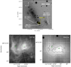 |
Fig. 1. Top row: NGC 2366, with labeled major substructures and the PMAS field of view. Figure reproduced from Micheva et al. (2017b). Bottom row: continuum-subtracted Hα images from the HST (left panel) and PMAS (right panel). The positions of knots A and B are indicated with open circle and open square, respectively. HST Hα iso-intensity contours at 8.1 × 10⁻⁶, 1.3 × 10⁻⁶ and 1.9 × 10⁻⁷ erg s cm−2 Å arcsec−2, are overplotted on the PMAS image for orientation. The position angle of the HST field is rotated by ∼14 deg relative to the PMAS image. |
The layout of the paper is as follows. In Sect. 2 we present the PMAS observations, reductions, and final data product. The Hα kinematics are analyzed in Sect. 3, and we take a closer look at the spatially resolved physical conditions in Sect. 4. A discussion of the observational results and comparison to simulations in presented in Sect. 5, and the conclusions summarized in Sect. 6. Appendices A and B contain details about the reductions and the continuum subtraction of auxiliary narrowband imaging, respectively. Throughout this paper, the AB magnitude system is used.
2. IFU observations of Mrk 71
We obtained 2 × 1800 seconds of on-target exposure with the fiber-fed Potsdam Multi-Aperture Spectrophotometer (PMAS; Roth et al. 2005) at the Calar Alto 3.5m telescope during the night of March 25th 2017 (PMAS run362). We used a setup similar to the observations presented in Herenz et al. (2016), namely, the R1200 backward-blazed grating with the Lens Array (LArr), with a field of view of 16″ × 16″ in double magnification mode. Arc and continuum lamp calibration and bias exposures were taken at the same position in the sky, before and after the Mrk 71 exposures, as well as a separate sky exposure of 300 s, taken between the two Mrk 71 exposures, and offset by 1 deg in right ascension and declination from the Mrk 71 coordinates. The spectro-photometric standard star G191B2B (Oke 1990) was observed for the purpose of flux calibration, with arc lamp, continuum lamp, and bias exposures taken at its position in the sky. For the duration of the observations, the sky conditions were clear and stable. The observation summary is shown in Table 1.
Observation summary for the night of 2017-03-25.
2.1. Data reduction and calibration
The data were reduced following the recipe outlined in Sandin et al. (2010) and Herenz et al. (2016), using the p3d-package1 (Sandin et al. 2010, 2012). The reduction steps are given in detail by these authors, and we only summarize them briefly below. A master bias was created from average stacking of five bias images with the p3d-subroutine p3d_cmbias. Care was taken to select only those frames which had the same median bias level as that measured in the overscan regions of each science frame and each chip. The p3d subroutine p3d_ctrace was then used to obtain a trace mask for each science exposure from the associated continuum lamp exposures. Similarly, individual dispersion masks were obtained for each science exposure from the associated arc lamp observations, using the subroutine p3d_cdmask. The resulting wavelength sampling was 0.46 Å per pixel. We used the modified optimal extraction (MOX) setting with the subroutine p3d_cobjex to extract the spectra. Cross-talk contamination between neighboring spectra for the LArr IFU is negligible, and we have not applied a correction, as recommended by Sandin et al. (2010). A correction for fiber-to-fiber throughput variations was applied by flatfielding the data. Individual flatfields for each science and arc lamp frames were created from the associated continuum lamp observations, using the p3d_cflatf subroutine.
The same reduction and extraction procedures were applied to the standard star data. A sensitivity function was then obtained from the latter, using the subroutine p3d_fluxsens. Here we assumed the standard airmass extinction curve at Calar-Alto (Table 5 in Sánchez et al. 2007). The science exposures of Mrk 71 were then separately flux calibrated using this sensitivity function. The final data product is a data cube of 16 × 16 × 3991 volume pixels (voxels), with a spatial sampling of 1″ × 1″ spatial pixels (spaxels), and with spectral sampling of 0.46 Å per pixel, covering the wavelength range from 5825 to 7650 Å. The wavelength calibration has an absolute accuracy of 0.1, 0.05, and 0.07 Å at λ = 5850, 6500, and 7440 Å, respectively, which corresponds to an accuracy of ±5, ±2.5, and ±2.8 km s−1. These uncertainties were obtained by measuring the wavelength at the peak position of HgNe arc lines at the indicated wavelengths, and taking the average offset between these measurements and their theoretical values. Vignetting at the blue and red ends extends to ±350 Å (Roth et al. 2010), and makes those parts of the array unusable. This affects the He Iλ5875.6 and [O II] lines, for which the first and last 16 fibers along the spatial direction in the row-stacked spectra2 are affected by vignetting and not used in the analysis. These fibers are mapped to the first and last columns of the 2D spatial array.
We examined the effect of differential atmospheric refraction (DAR) with the subroutine p3d_darc. At the bluest and reddest wavelengths of our spectra, the DAR correction amplitude reaches at most 0.1″, which is negligible compared to our resolution of 1″ per spaxel. We therefore omitted applying a DAR correction in order to avoid another interpolation of the data.
2.2. Calibration of the second order [O II] λ3727 emission
Our data were taken with the PMAS setup intended for observations of the extended Lyman α Reference Sample (eLARS; Herenz et al., in prep.; Bridge et al., in prep.). The redshifts of the eLARS galaxies are such that a UV-blocking filter was not inserted, because the second order contamination by UV lines like [O II] λ3727 is redshifted outside of the spectral window. Mrk 71 is, however, at a distance of only 3.4 Mpc, and therefore a second order spectrum of the UV [O II] doublet is indeed present at the expected position of 2 × λ = 7454 Å and with twice the doublet wavelength separation.
The second order contamination of the UV [O II] is treated as a fortuitous feature throughout this work. We flux calibrate the UV [O II] doublet with HST imaging in F373N from the archive (PID 13041, PI: B. James). The HST filter contains both doublet lines, and therefore we can only calibrate the sum of [O II] λ3726 + 3729. The standard reduction steps described in Sect. 2.1 do not account for the fact that the second order UV spectrum needs to be flatfield corrected with a UV flatfield. With the second order UV arc lamp line of Hgλ3650.14 Å, we create the UV sensitivity map shown in Fig. A.1 in the Appendix, and use it to flatfield the UV [O II].
2.3. Sky subtraction
The sky subtraction method that gave the lowest residuals at line center was directly subtracting the available sky exposure, although due to the shorter exposure time of the latter, this increased the noise in the continuum of the sky-subtracted spectra. We only aim to reliably trace the gas emission lines, and therefore the increased noise in the continuum and in the outskirts of the field of view is of no consequence to our analysis. In addition, we tested other methods for removing the sky emission. We tried modeling the sky lines with Gaussian functions and the sky continuum with a low order polynomial and subtracting the composite model from each spectrum, and also modeling and subtracting only the sky continuum, and accounting for sky lines by fitting them simultaneously with the gas emission lines. These methods performed worse, and we opted for directly subtracting the flux-calibrated sky exposure from the two science exposures as the best method of removing sky emission. The science exposures were average-stacked after the sky subtraction.
2.4. Measurement of gas emission lines
We identified the following lines in the first order spectra of Mrk 71: He Iλ5875.6, λ6678.1, λ7065.19, O Iλλ6300, 6363, [S III] λ6312, [N II] λλ6548, 6584, Hα, [S II] λλ6716, 6731, [Ar III] λ7135.8, [O II] λλ7320, 7330. Figure 2 shows the full spectral range and labeled lines for our target. The second order spectrum is labeled as UV [O III]. Columns with index x = 0 and x = 15 are affected by vignetting in the wavelength range λ ≲ 6175 Å and λ ≳ 7300 Å respectively. Throughout the analysis, these columns are discarded for the emission lines that fall within these wavelength ranges.
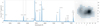 |
Fig. 2. Sky-subtracted and flux-calibrated average spectrum from the PMAS data cube (left panel) of the region marked in the Hα intensity map (blue circles in right panel, at the center of each spaxel). All identified lines are labeled, including the UV [O II] second order spectrum. The sky emission at [O I] λλ6300, 6363 (gray dashed lines) could not be fully subtracted with the sky exposure. The y-axis is truncated in order to better show weak lines like [O II] λλ7320, 7330. Vignetting affects the regions λ ≲ 6175 Å and λ ≳ 7300 Å at the edges of the detector (columns x = 0 and x = 15). |
The flux, width, and central wavelength of each line, along with the uncertainties in these quantities, were obtained via Monte-Carlo (MC) simulations in the following way. The p3d subroutine p3d_ifsfit measures the flux, full width at half maximum (FWHM), and the wavelength at line peak by fitting a Gaussian function to the line, where the position, amplitude and width of the lines are allowed to vary during the fit. This first estimate provides fitting errors for each quantity. In each MC run, we perturbed each spectrum by adding random noise to each line spectrum, drawn from the (assumed normal) distribution of the original p3d_ifsfit error. Each perturbed spectrum was passed to p3d_ifsfit to obtain the flux, width, and central wavelengths for that MC run. For a given spectrum, the average of 1000 MC realizations are taken as our best estimates of the line flux, FWHM, and wavelength. For each of these properties, the standard deviation of the distribution of 1000 MC runs is taken as the associated 1σ uncertainty.
Despite our sky subtraction, residuals of the oxygen sky emission lines at 6300 and 6363 Å remained. Due to the low redshift of Mrk 71, these lines are only ∼ 1.5 Å away from the [O I] nebular emission lines of our target. For these two cases, we therefore fitted the residuals of the sky lines simultaneously with the target lines.
2.5. Resolving power
To obtain the instrumental line broadening for every line and every spaxel, we used the subroutine p3d_ifsfit on the wavelength-calibrated arc lamp exposures to measure the widths of all arc lamp lines in every spaxel. We have defined the resolving power as R = λ/Δλ, where Δλ = FWHM. A total of 26 HgNe lines in the range 5852 − 7536 Å were fitted with Gaussians. In order to obtain resolving power maps at the wavelengths of the gas emission lines of our target, we fitted a sixth order polynomial to the arc line widths to enable interpolation. This is illustrated in Fig. 3a, where for plotting purposes we have stacked all spectra in each column in order to avoid cluttering. A resolving power map at the wavelength of Hα is shown in Fig. 3b. At this wavelength the median vFWHM is 63 km s−1, corresponding to a resolving power of  of 4704.
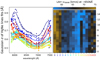 |
Fig. 3. (A) Instrumental broadening for 26 HgNe arc lines (filled circles), here for representation purposes obtained by stacking the spectra along columns in (B). The data points and the ID of the column that produced them have the same color-coding. The colored solid lines are a sixth order polynomial fit, used to interpolate the resolving power at the desired wavelength. (B): An example resolving power map close to Hα. The x-axis shows the column ID, color-coded as in (A). |
2.6. Internal reddening correction
In order to correct our spectra for internal dust extinction in Mrk 71 we use archival HST data. This is necessary, since our spectral range does not cover the Hβ line. To map the dust in Mrk 71 we use available HST imaging in F656N (Hα), F487N (Hβ), F814W (Hα continuum) and F438W (Hβ continuum) from the archive (PID 13041, PI: B. James). A continuum scaling factor for each filter, constant across the field of view, was obtained with the mode method (Keenan et al. 2017), using the residual mode representation of Micheva et al. (2018) to identify the scaling factor. Further details on the mode method are provided in Appendix B of the Appendix. Ideally, one would want to determine a spatially resolved scaling factor, in order to account for possible color gradients due to different stellar populations. This can be done by modeling the spectral energy distribution (SED) at each spaxel and from the model determining the continuum at line position (e.g., Hayes et al. 2009). We choose to use the mode method because it is simpler, the dust reddening is known to be overall low in Mrk 71 (e.g., Izotov et al. 1997), and none of our results rely crucially on a highly accurate reddening correction.
Once obtained, the continuum-subtracted Hα/Hβ map is then convolved with the average seeing of our observations (1.7″, Table 1), and resampled to the resolution of PMAS of 1″ per spaxel, using the python package reproject (Robitaille et al. 2016). Mode residual plots, indicating the scaling factors for Hα and Hβ, are shown in Fig. B.1, and the resulting reddening map is shown in Fig. B.2 in the Appendix. Continuum-subtracted Hα contours are overplotted, tracing the 8.1 × 10⁻⁶, 1.3 × 10⁻⁶ and 1.9 × 10⁻⁷ erg s cm−2 Å arcsec−2 iso-intensity levels. The location of the two super star clusters, knots A and B, discussed at length in Micheva et al. (2017b), are indicated for orientation.
The Hα/Hβ map is used to correct the spectrum in each spaxel for internal reddening. We assume the Cardelli et al. (1989, RV = 3.1) reddening law and use the python software pyneb (Luridiana et al. 2015) to obtain the reddening correction at each wavelength for case B recombination (Te = 104 K, ne = 100 cm−3). We will measure Te and ne explicitly in Sect. 4.1, however, the dependence of Hα/Hβ on the temperature and density is weak, and the dust map we obtain should not be significantly affected by departures from the assumed Te and ne values. For now we note that, assuming the same reddening law, the resulting extinction correction c(Hβ) is consistent with the literature, suggesting that our continuum subtraction is acceptable. For example, with the Fitzpatrick (1999) reddening law, at knot A we obtain c(Hβ) = 0.31, while James et al. (2016) reported 0.2 − 0.35, using a spatially resolved continuum scaling factor. A consistent value was obtained from Gonzalez-Delgado et al. (1994), using long-slit spectroscopy. For the region around knot B our dust map shows no dust, with Hα/Hβ ratios below 2.86. This is consistent with a long-slit spectroscopy measurement by Izotov et al. (1997), who find c(Hβ) = 0.01 for knot B.
3. Kinematics
To investigate the kinematics, we use the Hα line, which is the strongest observed line in our wavelength range and has high S/N > 10 is all spaxels.
3.1. Velocity field
The radial velocity of the gas in the line of sight is obtained in the usual way, by measuring the offsets of the line peak and comparing to its restframe wavelength, v = cΔλ/λrest. As a reference zeropoint, we take the luminosity-weighted average of ⟨ v ⟩ = 95.34 km s−1. The resulting velocity map is shown in Fig. 4a. The location of knots A and B, as well as HST continuum-subtracted Hα contours are overplotted for reference, with the faintest (outer most) contour defining what we consider the “core” region of Mrk 71. We observe a velocity gradient, which is likely a combination of the velocity field of the host galaxy (e.g., Hunter et al. 2001) and the presence of a biconical outflow, which we will discuss in the next sect. 3.2. A wide band of close-to-zero relative velocity, (white spaxels in Fig. 4a), reminiscent of a kinematical axis, runs through the entire field of view, along an approximately east-west direction, and varies in width between 16.5 pc to the west, 116 pc at the location of Knot A, and 66 pc to the east. Since the field of view covers only Mrk 71, which is a part of the larger parent galaxy NGC 2366 (e.g., Noeske et al. 2000)3, the observed velocity field is difficult to interpret in terms of lack or presence of rotation.
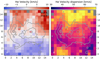 |
Fig. 4. (A): Hα radial velocity distribution around the luminosity-weighted average velocity zero-point of 95.34 km s−1. HST Hα countours are overplotted in gray solid lines, with the outer most (faintest) contour tracing the 1.9 × 10⁻⁷ erg s cm−2 Å arcsec−2 iso-intensity level. (B): Hα velocity dispersion, corrected only for instrumental broadening. Only spaxels with S/N ≥ 10 are shown. The gray spaxels at positions (0,14) and (8,15) are dead fibers. |
To estimate the large-scale motion of the gas, we measure the shearing velocity as vshear = (vmax − vmin)/2. Following Herenz et al. (2016), we take the median of the upper and lower fifth percentile of the velocity values to obtain vmax and vmin, and propagate the full width of each percentile to estimate conservative uncertainties on vshear. We obtain vshear = 9.6 ± 3.0 and 5.7 ± 0.9 km s−1 for the full field of view and for the region inside of the overplotted contours in Fig. 4, respectively, with measurements for additional regions tabulated in Table 2. For such low shearing velocities to be compatible with typical vmax of Hα rotation curves of spiral disks (e.g., Epinat et al. 2010), the inclination would have to be close to zero, that is, a face-on disk. The morphology of Mrk 71 in Fig. 1 is, however, clearly not reminiscent of a face-on disk. As previously mentioned, Mrk 71 is part of a larger host galaxy, which may have substantially higher vshear. We deduct that Mrk 71, taken in isolation from its parent galaxy, does not manifest a disk structure, and if such structure exists, it is not compatible with typical local rotators. Similar inconsistencies in implied vmax were observed for the LARS sample, most of which has complex velocity fields and too low vmax by a factor of more than two compared to typical rotator samples (Herenz et al. 2016).
3.2. Velocity dispersion
The velocity dispersion is similarly obtained from the observed broadening of the line,  , where FWHM is the full width at half maximum of the line. The resulting velocity dispersion map is shown in Fig. 4b, corrected only for instrumental broadening. A spatially resolved thermal broadening correction is applied in Sect. 4.3, and does not change the observed pattern. Two regions to the north and to the south show clearly elevated values of σ, suggestive of the presence of an outflow. A blowout and outflow, coincident with the location of the north region of increased σ, has been detected via HST nebular imaging (e.g., James et al. 2016), spatially resolved [OIII] kinematic data (e.g., Roy et al. 1991), and H I mapping (e.g., Hunter et al. 2012). As pointed out in Micheva et al. (2017b), knot B appears to be the cause of a superbubble, with shell morphology to the east, and the blowout region to the north. This is consistent with the location of knot B being at the apex point of the seemingly conical region of higher σ to the north. Such a conical structure is similar to that of a perturbation, propagating downstream in a supersonic flow, as we discuss in more detail in Sect. 4.4. This region also overlaps with a corridor of high [O III] 5007/[O II] 3727 ratios ≥10, indicating gas with high degree of ionization, and reaching the outskirts of Mrk 71 (Micheva et al. 2017b, their Fig. 4).
Comparing to Fig. 4a, we note that the north and south regions of high σ show redshifted and blueshifted velocities, respectively. Further, the HST continuum-subtracted Hα contours, overplotted on the image, show extended “fingers” of Hα emission connecting to both high-σ regions, and likely a product of the gas being swept up by the outflowing gas. We cannot investigate the southern region in any greater detail as we are limited by the field of view. However, taken at face value Fig. 4b suggests that the outflow, first detected by Roy et al. (1991), may be biconical. The hot young stars, capable of providing significant mechanical feedback in the form of stellar winds, as well as expanding supernovae remnants, are likely to be located inside of Mrk 71, and not in the outskirts, where the increased velocity dispersion σ is observed. Therefore the regions with higher σ to the north and south must be due to a sudden drop in the gas density.
The reasoning behind this conclusion is as follows. The total velocity dispersion can be the result of both thermal and turbulent contributions. The strong anti-correlation of the temperature with gas density yields a higher thermal velocity dispersion in low-density gas. For the turbulent component we also expect smaller dispersions for higher densities. Dense regions condense out of the diffuse warm gas and consequently correspond to a contraction from large to small scales. Turbulence – and thus the turbulent velocity dispersion – cascades down from large to small scales with a strong inverse scaling of the dispersion as a function of density. As both thermal and turbulent velocity dispersions follow the same trend we expect an anti-correlation of σ with the density, irrespective of the relative weighting between the two components.
In this context we can also compute the vshear/σm ratio, which is an indication of whether the gas is dominated by chaotic or ordered motion. As a representative velocity dispersion of the region we take the intensity-weighted local mean of the resolved velocity dispersion, ⟨σm⟩ = ∑σiIi/∑Ii (e.g., Östlin et al. 2001; Green et al. 2010; Glazebrook 2013). Since Mrk 71 is a giant H II region, part of a larger parent galaxy, we expect dispersion-dominated kinematics, and hence a ratio vshear/σm < 1. Indeed, the tabulated values in Table 2 for the full field of view, and for regions defined in Fig. 5, are indicative of kinematics dominated by turbulence.
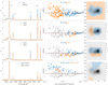 |
Fig. 5. Left column: Averaged spectra for different spatial regions, in arbitrary flux density units, scaled to match in Hα equivalent width. The continuum has been subtracted from both the blue and orange spectra, enabling comparison between panels in different rows. Middle column: Intensity-velocity dispersion diagrams for Hα. The horizontal line in each panel is 〈σm〉. Markers are color-coded by the spatial location of their corresponding spaxels, shown in the right column. We note that the y-axis values are di played on the right-hand side. Right column: Spatial maps of Hα, identifying the different regions. North is up, east is to the left. |
3.3. Is there a broad component?
A faint and very broad velocity component of FWHM = 45 Å has been detected by Roy et al. (1991), and confirmed by Gonzalez-Delgado et al. (1994), but with FWHM = 30 Å. This velocity component has been reported as centered on a cavity in the Hα emission, near knot A. The nature and acceleration mechanism of this component is still not known, as there are problems with every scenario for its origin: Thompson scattering by hot gas, superbubble blowout, stellar winds, supernova remnants (Roy et al. 1992), and turbulent mixing layers (Binette et al. 2009).
To facilitate our discussion, in Fig. 5 we divide Mrk 71 into several regions. We aim to spatially map and identify differences in the properties of the ionized gas, but other than knowing the location of the two super star clusters (SSCs) knots A and B, we have no prior notion of the extent of any regions, manifesting different properties. We therefore simply divide Mrk 71 into the somewhat arbitrary regions of “east”, “west”, “north” and “south”. The extent of the regions is arbitrary in the sense that no physical criteria were applied in the selection of included spaxel, and neighboring spaxels were excluded if, for example, a residual cosmic ray was present near the Hα line. The “core” region contains most spaxels inside the outermost Hα contour. We also added two regions with the spaxels covering the elevated velocity dispersion in the north and in the south.
In Fig. 5 we juxtaposition the average-stacked spectra of these regions in the left column, plot them in an intensity – velocity dispersion diagram in the middle column, and show their spatial location in a 2D map in the right column. The color-coding is intended to facilitate quick identification of the regions across columns. For example, in the first row the average-stacked spectrum of the core region is shown in blue, and in the second and third columns blue markers represent data from spaxels inside of that region.
Some obvious differences and features in the spectra are immediately apparent. The shape of the Hα profile varies across regions, which we examine in detail in the discussion (Sect. 5). The west region has stronger high ionization lines (He Iλ6678) and weaker [S II] λλ6716, 6731, compared to the east. This is consistent with the higher excitation and presence of younger massive stars in knot A compared to B (e.g., Gonzalez-Delgado et al. 1994; Drissen et al. 2000; James et al. 2016; Micheva et al. 2017b). Further, high ionization gas, traced by He Iλ6678, seems to be present also outside of the core region, as shown in row four for the high σ north and south regions. This is consistent with the presence of optically thin gas in the outskirts of Mrk 71, detected via ionization parameter mapping with [O III] λλ4959, 5007/[O II] λ3727 (James et al. 2016; Micheva et al. 2017b).
Figure 5 illustrates that a broad component is indeed present. The left column of the figure demonstrates that the core region has significantly broader Hα emission than the “outskirts” (row one). Dividing the core into east and west as indicated in the figure, one can further see that the Hα line is broader in the west region than in the east (row two). Dividing the core into north and south regions instead decreases the difference between the Hα line widths (row three), but both profiles appear broader than the outskirts region in row one. The broad component is entirely undetectable in row four of the figure, where the northern and southern high velocity dispersion regions are juxtapositioned instead. Thus, the broad component is most prominent in the core of Mrk 71, and more precisely in the western, circularly-shaped region marked in the second row of the figure. This region encompasses knot A, but is not centered on it. It is also apparent that the broad and narrow velocity components are decoupled from each other, in the sense that the high velocity dispersion northern and southern regions (row four) do not have a detectable broad component.
3.4. The I-σ diagnostic
Munoz-Tunon et al. (1996) suggest that an intensity versus velocity dispersion diagram can help identify the main line broadening mechanism, caused by, for example, expanding shells and loops generated by the winds of massive stars. The I-σ diagnostic uses the fact that when fitting line profiles with a single Gaussian regardless of the shape of the line, the fit will conserve the flux. As a consequence, strongly-split and very asymmetric line profiles will result in a fit of lower peak intensity but broader shape. This can be used to identify line fits with low intensity and broad shapes. If spatially clustered together, such points suggest a region of very asymmetric and split emission lines, which are usually the signatures of the expansion of the gas in shells, rings, bubbles. In the I-σ parameter space such regions will appear as “inclined bands”, because the broader the line appears, the lower its peak flux. We construct such a diagram in the middle column of Fig. 5, but we use the modified presentation of Moiseev & Lozinskaya (2012) with log I being the integrated flux of the line, and not the peak intensity. This has the advantage of being independent of the spectral resolution. Here we use the velocity dispersion σ, shown in Fig. 4b, corrected only for instrumental but not thermal broadening. The horizontal line in these plots is the intensity-weighted local mean velocity dispersion, ⟨σm⟩, defined in Sect. 3.2.
In this diagram, we see the typical horizontal lane of σ ≈ ⟨σm⟩, made up of the majority of spaxels in the core region. In our case, this ⟨σm⟩ = 50.7 km s−1 corresponds, within errors, to the minimum line width, observed in the core region (Fig. 5A). Such behavior is consistent with the Munoz-Tunon et al. (1996) interpretation of this diagnostic. This value should be close to the stellar velocity dispersion, σ⋆. In addition to the horizontal lane, we observe lower-intensity points with both higher and lower σ. According to the model schematics of Munoz-Tunon et al. (1996, their Fig. 6), this implies that the expanding shells and loops around massive stars have breached the “kinematic” core of Mrk 71, and are expanding beyond its borders. The spatial map of the velocity dispersion, with the overplotted Hα contours in Fig. 4b, is clearly consistent with such a scenario. While it is difficult to identify new, previously undetected, expanding shells or loops with this diagnostic at our course spatial resolution, we see that the high σ north and south regions (row four), indeed appear as inclined bands in this diagram. At least the northern region has been previously identified as a blowout region by, for example, Roy et al. (1991).
Finally, in the model of Munoz-Tunon et al. (1996), the smaller scatter of the west region points in Fig. 5B suggests that the west region, hosting knot A, is dynamically younger than the east region, hosting knot B. This is consistent with the younger age of knot A compared to knot B.
4. Physical conditions
4.1. Electron temperature and density
The density-sensitive [S II] ratio can be used to map the electron density at each spaxel. The fortuitous presence of a second order spectrum of the UV [O II] doublet enables us to also calculate an electron temperature map using the temperature-sensitive [O II] λ3726 + 3729/[O II] λ7320 + 7330 ratio. Using the python software pyneb (Luridiana et al. 2015), we cross-converge the temperature (Te) and density (ne) from both diagnostics with getCrossTemDen. To obtain robust estimators for these quantities and their uncertainties, we perform 1000 Monte Carlo runs, at each realization perturbing the spectra in the manner described in Sect. 2.4, and obtaining a new Te and ne after re-measuring the line ratios. The average Te and ne of these realizations are presented in Fig. 6, and listed in Tables 3 and 4 for different regions. Due to the non-parametric nature of the resulting distributions, the associated uncertainties in each spaxel are estimated as the root mean square (rms) of the 1000 Te and ne values. For the case of the electron density, spaxels in the low-density limit but inside of the high signal-to-noise (S/N) region, indicated by the overplotted contours in the figure, are explicitly set to the lowest physical value of [S II]λ6731/6716 ∼ 0.69.
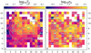 |
Fig. 6. (A): Electron temperature log10Te[K]. Knots A (green open circle) and B (green open square), as well as Hα contours are overplotted for orientation. Numbers indicate relative error, with “0.1” corresponding to 0.1 ≤ δTe/Te < 0.2, etc. Spaxels with no numbers have δTe/Te < 0.1. (B): Electron density log10ne[cm−3]; same legend as in (A). Both Te and ne are obtained with pyneb. |
The temperature-sensitive [O II] λ3726 + 3729/[O II] λ7320 + 7330 ratio spans a very wide wavelength range, and so is dependent on how accurate the internal extinction can be estimated. In Sect. 2.6 we obtained Hα/Hβ from HST imaging, using a constant scaling factor to subtract the continuum in each filter. While our reddening map is consistent with the literature, it is worth considering the effects on the electron temperature that under- or overestimating the extinction correction c(Hβ) would have. If one underestimates c(Hβ), the UV [O II] flux will be more strongly affected than the [O II] doublet at 7325+Å, the temperature-sensitive [O II] ratio will be underestimated, and hence the electron temperature will be overestimated.
We therefore compare our Te and ne maps with results from long-slit spectra in literature. For the spaxel containing knot A, Te = 13374 ± 116 K, and ne = 273 ± 17 cm−3. Similar values obtained from the same line ratios are found in the literature, suggesting that our unusual procedure for obtaining the Te map has nevertheless been successful. For knot A, Sokal et al. (2016) measure Te([O II]) = 1.3 ± 0.3 × 10⁴ K, and Gonzalez-Delgado et al. (1994) obtain Te([O II]) = 1.45 ± 0.13 × 10⁴ K, both consistent with our measurement within the uncertainties. Similarly, ne = 512 ± 264 cm−3 in Sokal et al. (2016), and ne = 235 ± 41 cm−3 in Gonzalez-Delgado et al. (1994), also both consistent with our measurement. We also obtained an electron density map from the UV [O II]3726/3729 ratio, which gave ne = 287 cm−3 for knot A – a result consistent with that obtained from the [S II] ratio.
The electron density map is quite noisy. A noticable increase in ne is observed around knot A, which is likely real, given its location (knot A is an embedded super star cluster). The spaxels with similarly high ne found in the outskirts of the image, however, are more reminicent of salt-and-pepper noise, than real features. Taken at face value, the electron density map shows densities typical for H II regions over the entire field of view.
As can be seen in Fig. 6, the dominant trend in Te presents a vertical pattern, with Te being significantly higher to the north around knot A than in the south. The observed change in temperature across Mrk 71 in the figure may be due to metallicity variations on the same spatial scales – a scenario investigated by James et al. (2016). We are unable to verify this, as none of the [O III] lines are in our spectral coverage, and therefore we cannot use the so-called “direct” Te method to determine the oxygen abundance. Additionally, Kewley & Dopita (2002) demonstrate that metallicity-sensitive strong-line method ratios like [N II]/[O II], [N II]/[S II], or [N II]/Hα, all within the spectral range of our data, become insensitive to the metallicity at Z ≲ 0.5 Z⊙. Since Mrk 71 is metal-poor (12 + log O/H = 7.89 ± 0.01; Izotov et al. 1997; Hunter & Hoffman 1999), the “strong-line” method involving these lines also cannot be used to obtain spatially resolved metallicity.
However, at a projected separation of 5 arcsec, the two knots A and B have very similar oxygen abundances of 12 + log O/H = 7.89 ± 0.01 and 7.85 ± 0.02, respectively, measured using the “direct” method on data from long slit spectra (Izotov et al. 1997). Gonzalez-Delgado et al. (1994) also find no significant variation in the oxygen abundances from spectra extracted from 15 positions, including knots A and B, from long slit observations. This is expected, since they are also unable to find significant Te gradients for these positions, because their temperature uncertainties are quite large and their slit positions generally avoid the low-temperature regions. Further, James et al. (2016) use HST narrowband imaging and the R23 index (“strong-line” method) to obtain a map of 12 + log O/H in a 5″ × 5″ region, covering knot A. Within the uncertainties of their measurement there is no convincing trend in the spatial metallicity distribution. Although discrepancies in temperature between the “strong-line” and “direct” Te methods are expected, relative variations would be traced by both. Therefore, the observed seeming variation in the electron temperature may reflect true differences in the physical conditions of the gas. The highest observed Te coincides with the location of knot A, where numerous evidence points to the possible existence of very massive stars (e.g., James et al. 2016; Micheva et al. 2017b). The high Te is likely the result of the very high ionization parameter of log U= − 1.89 ± 0.3 and the associated extremely high ratio of [O III]λ5007/[O II]λ3727 = 23.0 at knot A (Micheva et al. 2017b). This is consistent with the observed elevated Te in the north (Fig. 6a), in a region which also shows high [O III]λ5007/[O II]λ3727 ratios (James et al. 2016).
Nevertheless, none of these arguments convincingly demonstrate that there is no metallicity variation across Mrk 71, giving rise to the observed seeming variation in electron temperature. In particular, the south region, defined in Fig. 5, is not covered by either the Izotov et al. or the James et al. metallicity measurements, and only partially covered by the Gonzalez-Delgado et al. data.
4.2. Speed of sound
The electron temperature map enables us to spatially map the speed of sound across the field of view, given by  (Osterbrock 1989). This is the speed at which pressure waves travel in a hydrodynamical expansion of the region. We assume a completely ionized, isothermal, pure hydrogen H II region with adiabatic index γ = 1 and mean molecular weight μ ≈ 0.5. The resulting sound speed is largest at knot A (cS = 14.9 km s−1), with average, median, and brightest spaxel differences presented in Table 4 for the regions defined in Fig. 5. The spatial variation of cS is presented in Fig. 7a, and is in the range 7.6–14.9 km s−1, with an average of ⟨ cS⟩ = 10.5 ± 1.4 km s−1 from all spaxels in the field of view. This is a typical value for H II regions, at temperatures of Te ∼ 104 K. The statistics of cS for different regions are provided in Tables 3 and 4.
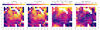 |
Fig. 7. (A): Speed of sound cS. Knots A (open circle) and B (open square) are given for orientation. (B): Thermal broadening. (C) “True” velocity dispersion, corrected for both instrumental and thermal broadening. (D) Mach number ℳ map, with strictly hypersonic regions (ℳ ≥ 5.0) marked with “x”. At knot B, ℳ = 4.63. |
4.3. Thermal broadening
Similarly to the speed of sound, one can obtain the thermal broadening of the emission lines, caused by the thermal motion of the gas,  . The thermal broadening ranges from 10.5 km s−1 at knot A, to 5.4 km s−1, with an average across the entire field of view of ⟨σthermal⟩ = 7.9 ± 1.0 km s−1. A map of the spatial distribution of σthermal is shown in Fig. 7b, with differences between regions tabulated in Table 4. Compared to Fig. 4b, some spaxels are missing data, but the overall pattern of increased velocity dispersion to the north and south is preserved. The missing data are due to the propagated missing data in the thermal broadening map, which in turn is due to the electron temperature map. The statistics of σthermal for different regions are provided in Tables 3 and 4.
4.4. Mach number
Explicitly obtaining the speed of sound and the thermal broadening allows one to map the Mach number ℳ = σtrue/cs, which is simply a measure of how fast the ionized gas is moving relative to the speed of sound. The “true” velocity dispersion, shown in Fig. 7c, is obtained as  , where σobs, σinst, and σthermal are the observed, instrumental, and thermal line broadening, respectively. The spatial distribution of ℳ, shown in Fig. 7d, has a range of 3.2 < ℳ < 7.5, with average ⟨ℳ⟩ = 4.6 ± 0.7, and hence the gas we trace is supersonic (ℳ > 1) over the entire field of view of 16 × 16 arcsec =112 × 112 parsec. The statistics of the Mach number for different regions are provided in Tables 3 and 4.
5. Discussion
In this section we use the nomenclature for different spatial regions, defined in Fig. 5, namely east, west, core, and we refer to the “high σ north” region simply as a region of increased velocity dispersion. NGC 2366, dominated by Mrk 71 in terms of star formation rate density and surface density of ionising photons, is the nearest GP analog and a candidate for LyC escape. At its distance of 3.4 Mpc, this galaxy offers the opportunity to analyze possible mechanisms and channels of LyC escape.
The proposed mechanism of LyC escape in NCG 2366/Mrk 71 involves the presence of optically thin corridors of lower gas density, through which LyC photons can reach the intergalactic medium (Micheva et al. 2017b). In this scenario, a SSC from an initial star-forming event (knot B in the case of Mrk 71), powers large-scale outflows via mechanical feedback. A consecutive star-forming event produces additional SSCs (knot A in Mrk 71), which ionize the remaining gas in the precleared region, in the process possibly carving optically thin corridors reaching beyond the outskirts of the galaxy. Knot B (age ≳5 Myr), has a population of Wolf-Rayet stars (Drissen et al. 2000; Sokal et al. 2016), whose strong stellar winds are capable of providing substantial mechanical feedback to preclear the region. Knot A is an extremely young (≲1 Myr) SSCs, still embedded in its natal cloud, and it dominates the ionization budget of Mrk 71 (Drissen et al. 2000). Very massive stars, younger than ≲1 Myr and with initial masses M⋆ ≥ 100 M⊙ (VMS; e.g., Crowther et al. 2010; Gräfener & Vink 2015), may be present in Knot A (James et al. 2016; Micheva et al. 2017b).
Neutral gas, which readily absorbs LyC photons, has been observed in NGC 2366, with line of sight N(H I) column densities of a few ×1021 cm−2 at the projected position of Mrk 71 (Hunter et al. 2001), which is prohibitively optically thick for the escape of LyC radiation. It is, however, unlikely that all of the observed H I gas lies in front of Mrk 71. Optically thin Si IIλ1260/λ1526 ratios, weak detections or non-detections of other low-ionization and neutral species, and low reddening in Mrk 71 (Micheva et al. 2017b), all suggest much lower absorption columns, and hence that most of the H I gas is behind Mrk 71. Additionally, ionization parameter mapping of Mrk 71 (James et al. 2016) shows high [O III]/[O II] ratios over most of the region, and stretching from the core to the north beyond the outskirts of Mrk 71 (Micheva et al. 2017b). Such ratios may also indicate optically thin gas (Jaskot & Oey 2013). Supporting this scenario is the spatially coincident outflow of ionized gas, detected with Fabry-Perot data (Roy et al. 1991), and also visible through an increase in velocity dispersion in our Fig. 4b.
Further evidence can be compiled from our own data. The region of observed increased velocity dispersion in Fig. 4b implies lower gas density. Additionally, the spatially resolved Mach number map in Fig. 7d shows that while all spaxels indicate supersonic gas (ℳ > 1), some spaxels even show hypersonic gas (ℳ ≥ 5). These are almost entirely found in the outskirts of Mrk 71, outside of the overplotted Hα contours of the core region. This boost in the relative gas velocity is a further indication of a drop in the gas density outside of the core.
Inside of the denser core region, the observed spatial distribution of the velocity dispersion allows one to identify knot B as the likely source of mechanical feedback which has cleared a channel of lower gas density reaching the outskirts. In a supersonic or hypersonic flow, a perturbation will generate sound waves, which propagate downstream and accumulate on a cone (Landau & Lifschitz 1987), whose surface is refered to as the shock front. A cone structure is visible in the velocity dispersion map in Fig. 4b, with knot B seemingly located at the apex of the cone. The aperture angle of the cone is 2α, where α is the Mach angle, sinα = cS/σ = 1/ℳ. At knot B ℳ = 4.63, and hence α ≈ 12.5 deg. Our spatial resolution prevents us from accurately tracing such a narrow cone. In Fig. 8 we have plotted the resulting cone aperture of 2α, approximately in the direction of the increased velocity dispersion. The velocity dispersion in this figure has been corrected only for instrumental broadening, in order to display as many spaxels with data as possible. We note, that the cone falls in the region of very low dust attenuation, which is shown by the overplotted Hα/Hβ contours. The seemingly biconical nature of the outflow, discussed in Sect. 3.2, supports the scenario of mechanical feedback from knot B being the cause of the low density channel, instead of the turbulent gas simply taking a preexisting path of least resistance. In the latter case a biconical structure, whose axis crosses the location of knot B, is less likely, although not impossible considering projection effects.
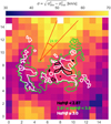 |
Fig. 8. Velocity dispersion, corrected only for instrumental broadening, with overplotted dust contours. The cone of 2× the Mach angle of downstream propagation of perturbations is also plotted for the Mach number at knot B (open square), ℳ = 4.63. The extinction outside of the plotted contours is negligible, see the reddening map in Fig. B.2. |
Since the Mach number is the ratio between true velocity dispersion and the speed of sound, both of which increase in turbulent, ionized regions, a wide range of Mach numbers can be obtained at a given gas column density (e.g., Girichidis et al. 2018, their Fig. 13). To estimate if the drop in gas density could be significant, we therefore compare our observations to available hydrodynamical simulations of the interstellar medium.
We use the recent high-resolution runs (Girichidis et al. 2018) of the SILCC4 simulations (Walch et al. 2015; Girichidis et al. 2016) for the comparison. The setup covers a fraction of a galactic disk in a volume of 0.5 × 0.5 × 0.5 kpc3 at a resolution of 1 pc. The magnetohydrodynamic simulations follow the thermal state of the interstellar medium using a chemical network including ionised, atomic and molecular hydrogen as well as C+ and CO with solar values for the metallicity. Radiation from stars is included as a backgroud radiation field, which is locally attenuated in regions of efficient shielding. Further stellar feedback is modeled via supernovae, where we distinguish between individual (1/3) and clustered (2/3) explosions. The stellar component is not modeled as individual stars. Instead we assume a stellar initial mass function (Chabrier 2003) and compute an effective star formation and resulting supernova rate based on the Kennicutt-Schmidt relation (Schmidt 1959; Kennicutt 1998). The dynamical features in the simulations are thus produced by the thermal energy injection corresponding to the supernovae. This is surely a simplification of the stellar feedback description. Gatto et al. (2017) and Peters et al. (2017) follow the dynamical formation of star clusters in dense and collapsing regions and include stellar winds and ionizing radiation from the star clusters with a maximum resolution of 4 pc. However, focusing on the global dynamics, the general conclusions of the comparison between simulations and observations is not altered by the additional physics in the latter two studies and we chose the simulations by Girichidis et al. (2018) because of the four times higher resolution.
We chose these simulations because of the similar column density and global turbulent dynamics, resulting in a similar range of measured velocity dispersion. Global galactic properties like the halo mass and the resulting dark matter distribution are not relevant for the ISM dynamics on scales of ∼5100 pc, which we are here investigating and comparing. Gravitational effects due to stellar masses might be comparable to the effects of self-gravity of the gas. The total mass of ≳1.6 × 10⁵ M⊙ in Mrk 71 (Micheva et al. 2017b) is comparable to the mass of a few 105 M⊙ in the selected region of the simulation.
The two main hypotheses in the interpretation of the observations we want to test, are (1) whether the physical properties of the conical outflow region are consistent with a significant enough decrease in density to enable LyC escape, and (2) whether the orientation of the conical outflow is along the plane of the disk, which would likely prohibit LyC escape into the IGM, regardless of density drop along the cone.
The first check against simulations concerns the density distribution in the region of increased velocity dispersion. Figure 9 shows one of the frequently appearing feedback features that is comparable to our observations. From left to right we show the total (ionized, neutral, and molecular) column density, the modulus of the line-of-sight (los) velocity, the los velocity dispersion, the thermal sound speed, and the Mach number. The top panels are the edge-on view of the galactic plane, the bottom ones depict the face-on view. Shown are the data after a total simulation time of 30 Myr, with the cluster formation time around ∼10 Myr. The white rectangle illustrates the region that is likely comparable to the observational field. We clearly note a region of low density, which has been evacuated by clustered stellar feedback in the disk. This cavity shows higher line-of-sight velocity and corresponding dispersion, as well as patchy enhanced sound speeds due to higher temperatures, all displaying values covering the range of our observations. The dispersion and sound speed increase in a correlated manner such that the Mach number only shows comparably small variations, quantatively similar to our observations in Figs. 7a, c, and d. Simultaneously, the column density shows on average a factor of ∼4 dex variations between the disk of the galaxy and the outflow region. Applied to our observations, even assuming all of the H I column density of ∼3 × 1021 cm−2 is in front of Mkr 71, which is unlikely, such a substantial density drop in the outflow region could imply column densities approaching ∼3 LyC optical depths, and hence a non-zero LyC escape fraction.
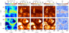 |
Fig. 9. High-resolution runs of the SILCC simulations (Girichidis et al. 2018). The white rectangle indicates the area comparable to our observations. Top row: edge-on projection of the galactic disk, the bottom panel one the face-on view. See Sect. 5 for details. |
The column density shown in Fig. 9 comprises the total density of gas, including ionized, neutral and molecular. In Fig. 10 we demonstrate that the density drop is dominated by the distribution of neutral H I – the gas phase of greatest importance for the fate of LyC photons. We also note that the simulations assume solar metallicity, while the metallicity of Mrk 71 is substantially subsolar at 12 + log O/H = 7.89 ± 0.01 (Izotov et al. 1997; Hunter & Hoffman 1999). However, for SNe the dynamical impact is not expected to be vastly different at lower metallicities. The energy injection would be the same, while simultaneously the cooling would be less efficient, which means overall more of the thermal energy could be converted into motions and the gas would stay warmer compared to the solar metallicity case.
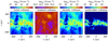 |
Fig. 10. Same as Fig. 9 but showing only the column density for the three considered gas phases. The white rectangle marks the region comparable to the observation. The column density range for the ionized gas is much smaller than for the other two components. The bright spot in the ionized column corresponds to a recently exploded supernova. |
The second hypothesis to test against simulations is related to the orientation of the cone with respect to the galactic plane of NGC 2366. How likely is the possible outflow cone pointing away from the plane? The numerical simulations suggest that enhanced coherent motions are more likely to appear out of the plane. A visual impression is evident by comparing the top and the bottom panels of Fig. 9. In both the upper and lower panels the low-density regions coincide with overall higher los velocities and velocity dispersions. However, for the lower panels, the correlation is much stronger indicating that the gas motions are much stronger perpendicular to the plane. A more quantitative analysis of this phenomenon is shown in Girichidis et al. (2018, their Fig. 6), over an evolutionary time of 60 Myr and multiple simulations. These authors show that for all simulations and over the entire simulation time, the isotropic motions are noticeably lower than the computed averages, which proves that the velocities pointing perpendicular to the galactic plane are dominating over the ones in the plane. Therefore, the interpretation that the observed cone in Fig. 8 is oriented out of the plane of the disk seems reasonable.
Additionally, the observed ionized outflow is not likely to be powered by an AGN. A Baldwin et al. (1981, BPT) diagram can be used to distinguish between star-forming galaxies (SFGs) and active galactic nuclei (AGN). We cannot construct such a diagram due to the lack of [O III] and Hβ (i.e., the y-axis of a BPT diagram), however, we can still examine the [N II] λ6584/Hα, and [S II] 6716 + 6731/Hα values (i.e., the x-axis of a BPT diagram). In a BPT diagram, AGN are typically found at log10[N II]/Hα ≳ 0.0 and log10[S II]/Hα ≳ 0.0. To be ambiguous and lie in the “composite” SFG/AGN region, these ratios would have to be ≳ − 0.6. In our PMAS data, all spaxels in the entire field of view have log10[N II]/Hα ≲ −0.89 and log10[S II]/Hα ≲ −0.6. The core region has ≲ − 1.0 and ≲ − 1.6, respectively, with averages −1.96 and −1.38. Such ratios place every spaxel in the extreme end of the BPT diagram, occupied by low metallicity SFGs. The same is true for line ratios, integrated over the entire Mrk 71 region, as shown in Micheva et al. (2017b). The BPT diagram in James et al. (2016), constructed from narrowband HST imaging, similarly shows all pixels to be well to the left of the theoretical SFG-AGN division line of Kewley et al. (2001). It is therefore unlikely that non-thermal radiation from an AGN is significantly contributing to the ionization of the gas, and is powering the outflow.
In summary, the kinematics and physical properties of the observed conical outflow region are much in line with being due to stellar feedback, are consistent with a significant drop in neutral gas density of ≲4 dex, and the outflow is likely pointing away from the disk. This is consistent with LyC escape, and under these conditions LyC photons can directly leak through the ISM, without the necessity for a “picket fence” ISM (Heckman et al. 2001; Bergvall et al. 2006), in which an otherwise optically thick ISM has a covering fraction of less than unity.
5.1. The broad kinematic component
In five GPs, Amorín et al. (2012) find broad Hα wings with complex, multigaussian components, indicating high-velocity gas (FWZI > 1000 km s−1). These wings are interpreted as a combination of multiple expanding supernovae remnants and strong stellar winds. Despite the much smaller distance to Mrk 71, the origin of the broad component identified in Sect. 3.3 is unknown. Our attempt to spatially trace it in individual spectra was unsuccessful, despite the high S/N in the Hα line. The reason for this is that relative to the peak of the Hα line, the broad component seems to be at the 0.2% level, and we do not have the S/N to trace such a faint component in most individual spaxels. We therefore average stack all spectra inside of the west region, which was identified in Sect. 3.3 as manifesting the strongest broad component. The resulting average-stacked spectrum is shown in Fig. 11 as a solid thick gray line in all three panels. Here we have normalized all shown spectra to an amplitude of unity in Hα. In Fig. 11a, we examine the possibility that the observed broadening is a result of the presence of a velocity field. Stacking spectra with line peaks offset from λrest may result in artificial broadening of the final spectrum (so-called “beam smearing”). To test this, we model each Hα line with a Gaussian, and then average stack the modeled profiles, to obtain the solid orange line in Fig. 11. The two [N II] lines are modeled simulteneously as Hα. Clearly, the resulting profile is much narrower than the observed Hα line (solid thick gray line), and the presence of a velocity field is not the reason for the broadening. In this same figure we also overplot the individual spectra (solid thin gray lines), which, while much noisier, all indicate a broadening wider than the averaged Gaussian model.
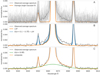 |
Fig. 11. west region average-stacked observed spectrum (thick gray line) around Hα, compared to (A) average-stacked single Gaussian models (orange line) and individual observed spectra (thin gray lines); (B) Empirical LSF (orange line) and LSF-convolved single Gaussian of various widths (blue lines); (C) composite model (orange line) of a broad Gaussian (green line) added to an LSF-convolved narrow Gaussian of width σ = 0.7 Å. |
Next, in Fig. 11b we consider the effect of the line spread function (LSF). We use average-stacked arc lamp lines at 6532.88 Å and 6598.95 Å from the same spatial region (west), and obtain an empirical LSF (solid orange line) at approximately the Hα wavelength by average stacking the two arc lines. We note that the wings of the LSF are much more Lorentzian than Gaussian. The effect of this LSF on a Gaussian profile can be seen by convolving Gaussian profiles with widths σ = 0.1 to 0.7 Å with the LSF, shown as solid blue lines in Fig. 11b. This is done for the Hα and the two [N II] lines simultaneously. None of the convolved profiles can account for the observed Hα wings below an amplitude of ≲0.003, or 0.3% of the Hα amplitude.
Finally, in Fig. 11c, we show a composite profile, consisting of a narrow Gaussian with σ = 0.7 Å for the three lines (Hα and two [N II] lines), convolved with the LSF, and added to a broad Gaussian of σ = 9.9 Å. This composite profile, shown in solid orange, is our best match to the observed Hα profile. The match is not perfect, but it is nevertheless clear that a broad component does indeed exist, and that Hα can be modeled with a two-component profile.
In contrast, the east region, containing knot B, can be modeled with a single Gaussian, convolved with the LSF, as demonstrated in Fig. 12. The average-stacked observed profile (solid gray line) is noisier here, and there appears to be some excess emission, localized around the [N II] 6584 line. This is likely a residual from the sky subtraction. In any case, a single Gaussian component appears to be sufficient to reproduce the profile of the observed Hα line.
In summary, we can confirm the presence of a broad component in Hα, previously reported by, for example, Roy et al. (1991). The averaged broad component in our data is highly localized to the west region, and is not broader than σ ∼ 10 Å, or a FWHM ≈24 Å∼1100 km s−1. This is narrower than the original detection by Roy et al. (1992), which had a FWHM of ≲2400 km s−1, and was later re-measured by Gonzalez-Delgado et al. (1994) with FWHM = 1400 km s−1 in the center at a 3% level of the narrow component, and ∼2800 km s−1 in the outskirts at a 30% level. The reason for the discrepancy with our value (∼1100 km s−1 at a < 0.3% level of the narrow component) is not certain, however, we can note that Gonzalez-Delgado et al. (1994) model the emission lines with Gaussians and do not mention accounting for the effect of the LSF, which may be non-Gaussian, as it is in PMAS. The insufficient S/N in the outskirts of our field of view prohibits the spatial tracing of this component on a spaxel to spaxel scale. This makes its further analysis difficult, and we remain ignorant of its origin and nature. We note, that in contrast to the complex fits with multigaussian components, required to explain the gas kinematics of GPs in Amorín et al. (2012), in Mrk 71 it is not necessary to add more than two Gaussian components to reproduce the observations. This is expected, since the multiple kinematical components in the GPs are likely due to multiple star-forming clumps (Amorín et al. 2012), while in Mrk 71 we resolve single star-forming regions.
5.2. Low- and high-ionization gas move in concert
Finally, we examine if different species, tracing neutral, low- and high-ionization gas, have the same velocities, using Hα as a reference line. If this is not found to be the case, this could imply local departures from thermal equilibrium, in which the rate of collisional excitation does not equal the recombination rate, or a projection effect of the 2D flattening of a complex 3D structure.
For every spaxel in the field of view, in Fig. 13 we plot the velocity obtained from the Hα line, versus the velocity of the low-ionization lines [N II] 6584 and [S II] 6716, and the high-ionization lines He I 5876 and [Ar III] 7136. These lines require ionizing photons with energies ≥1.1 and ≥0.8, ≥1.8, and ≥2.0 Ryd, respectively. Singly-ionized sulfur [S II] therefore traces the kinematics of neutral hydrogen, although its ionization potential is close to 1 Ryd, and hence it will also be found in low-ionization regions together with Hα. Most data points in Fig. 13 fall within ±5 km s−1 from the Hα velocity. Such small offsets of Δv ≲ 5 km s−1 from the 1:1 line can be attributed to a combination of the following systematics. The line spread function (LSF) varies across the field of view, with the profiles becoming more pronouncedly non-Gaussian toward the outskirts, which affects the peak position of their Gaussian models. We attempted to correct for this by modeling these instrumental systematics from HgNe arc lines in both the wavelength direction and in the two spatial directions, but found the S/N to be too low in individual spaxels of the arc line spectra in order to provide a significant decrease in scatter around the 1:1 line in Fig. 13. The uncertainty in the wavelength calibration additionally contributes from ±2.5 to ±5 km s−1 uncertainty at different wavelengths, as described in Sect. 2.1. Another consideration is that, other than the Hα line, the S/N of all other lines is significantly lower, making the determination of the Gaussian peak less accurate. This issue is compounded by the fact that our direct sky subtraction increased the noise significantly, making the most difference in spectra with already low S/N. At our minimum cutoff of S/N ≥ 15, the expected contribution to the uncertainty in the velocity is ∼2.5 km s−1, judging by the estimate of Herenz et al. (2016, their Fig. 4) for the LARS sample with an instrumental setup identical to ours. Finally, an additional source of scatter is possible stellar continuum absorption in certain regions of Mrk 71. While knot A is dominated by nebular continuum and would not be affected, knot B is a naked cluster with a stellar continuum clearly detected in, for example, Drissen et al. (2000) and Sokal et al. (2016). Other spaxels may also be covering regions, where the stellar continuum is not negligible. In such cases, underlying stellar absorption lines will influence the position of the peak amplitude of nearby emission lines.
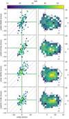 |
Fig. 13. Left panel: Hα radial velocity as a function of the radial velocity in lines tracing low-ionization ([N II], [S II]) and high-ionization gas (He I, [Ar III]). The points are color-coded by S/N. The 1:1 Hα velocity line (solid gray), with ±5 (dashed) and ±10 km s−1 (dotted) lines, are plotted for orientation. Only spaxels with S/N ≥ 15 or within the overplotted contours in the right panel are shown. Right panel: spatial distribution of the spaxels, color-coded by S/N. |
Therefore, we conclude that within the effects of instrumental systematics and possible stellar absorption, gas in different phases shows the same velocities. In particular, the data is consistent with neutral hydrogen gas moving together with the ionized gas, and hence the outflow detected in Mrk 71 via Hα and [O III] 5007 (Roy et al. 1991; Gonzalez-Delgado et al. 1994) is likely also present in H I. This is consistent with the simulation predictions in Fig. 10.
6. Conclusions
We present 5825 to 7650 Å PMAS IFU data of the giant H II region Mrk 71 in NGC 2366, the closest GP analog at a distance of only 3.4 Mpc. We obtain electron density and temperature maps, where for the latter we use a second order contamination by the [O II] λ3727 doublet.
We examine the Hα kinematics, and find evidence of a biconical outflow, with elevated velocity dispersion and redshifted (blueshifted) velocities to the north (south) of its apparent origin at the super star cluster knot B. An I-σ diagnostic verifies both regions as outflows or expanding shells. We verify and locate the previously detected broad velocity component in Hα from stacked spectra, and obtain a maximum full width at half maximum of 24 Å, or 1100 km s−1, at a maximum intensity of ∼0.2% of the narrow component. This is slower and fainter than the previous detections by Roy et al. (1992) and Gonzalez-Delgado et al. (1994). This component appears to be decoupled from the outflow regions, and its nature remains unknown, since it cannot be traced by individual spaxels.
We construct spatially resolved sound speed, thermal velocity dispersion, true velocity dispersion, and Mach number maps, and find evidence for a gas density drop outside of the core Mrk 71 region. These observational results are compared to high-resolution SILCC simulations, to demonstrate that the observed decrease in the gas density may be as large as ≲4 dex, even though the associated distribution in Mach numbers shows only minor differences between outflow and core regions. This implies almost optically thin H I column densities, and hence a non-zero LyC escape fraction in the direction of the outflow. This escape scenario does not require a H I covering fraction less than unity in order to enable LyC escape. We also verify that, within the systematic uncertainties, low- and high-ionization gas display similar velocities, and therefore likely move together.
Our results strongly indicate that kinematical feedback is an important ingredient for LyC leakage in GPs.
These are 2D arrays in which each row corresponds to an individual one-dimensional spectrum.
Mrk 71 is often misidentified as NGC 2363 in the literature, when in fact NGC 2363 is an interacting dwarf galaxy to the west of Mrk 71.
SImulating the LifeCycle of molecular Clouds.
Acknowledgments
We would like to thank Alaina Henry for refereeing this manuscript. We thank Christer Sandin, Lutz Wisotzki, Norberto Castro, Peter Weilbacher, Jakob Walcher, and Tanja Urrutia for enlightening discussions during the making of this paper. GM acknowledges support from the Leibniz-Wettbewerb, grant SAW-2016-IPHT-2. GÖ acknowledges support from the Swedish Research Council (Vetenskapsrådet) and the Swedish Space Board (Rymdstyrelsen). PG acknowledges funding from the European Research Council under ERC-CoG grant CRAGSMAN-646955.
References
- Alvarez, M. A., Finlator, K., & Trenti, M. 2012, ApJ, 759, L38 [NASA ADS] [CrossRef] [Google Scholar]
- Amorín, R., Vílchez, J. M., Hägele, G. F., et al. 2012, ApJ, 754, L22 [NASA ADS] [CrossRef] [Google Scholar]
- Baldwin, J. A., Phillips, M. M., & Terlevich, R. 1981, PASP, 93, 5 [NASA ADS] [CrossRef] [EDP Sciences] [Google Scholar]
- Bergvall, N., Zackrisson, E., Andersson, B.-G., et al. 2006, A&A, 448, 513 [NASA ADS] [CrossRef] [EDP Sciences] [Google Scholar]
- Bian, F., Kewley, L. J., Dopita, M. A., & Juneau, S. 2016, ApJ, 822, 62 [NASA ADS] [CrossRef] [Google Scholar]
- Binette, L., Drissen, L., Ubeda, L., et al. 2009, A&A, 500, 817 [NASA ADS] [CrossRef] [EDP Sciences] [Google Scholar]
- Bouwens, R. 2016, in Understanding the Epoch of Cosmic Reionization: Challenges and Progress, ed. A. Mesinger, Astrophys. Space Sci. Lib., 423, 111 [NASA ADS] [CrossRef] [Google Scholar]
- Bouwens, R. J., Illingworth, G. D., Oesch, P. A., et al. 2015, ApJ, 811, 140 [NASA ADS] [CrossRef] [Google Scholar]
- Brocklehurst, M. 1971, MNRAS, 153, 471 [NASA ADS] [CrossRef] [Google Scholar]
- Cardamone, C., Schawinski, K., Sarzi, M., et al. 2009, MNRAS, 399, 1191 [NASA ADS] [CrossRef] [Google Scholar]
- Cardelli, J. A., Clayton, G. C., & Mathis, J. S. 1989, ApJ, 345, 245 [NASA ADS] [CrossRef] [Google Scholar]
- Chabrier, G. 2003, PASP, 115, 763 [NASA ADS] [CrossRef] [Google Scholar]
- Chisholm, J., Orlitová, I., Schaerer, D., et al. 2017, A&A, 605, A67 [NASA ADS] [CrossRef] [EDP Sciences] [Google Scholar]
- Crowther, P. A., Schnurr, O., Hirschi, R., et al. 2010, MNRAS, 408, 731 [NASA ADS] [CrossRef] [Google Scholar]
- Dale, D. A., Cohen, S. A., Johnson, L. C., et al. 2009, ApJ, 703, 517 [NASA ADS] [CrossRef] [Google Scholar]
- Drissen, L., Roy, J.-R., Robert, C., Devost, D., & Doyon, R. 2000, AJ, 119, 688 [NASA ADS] [CrossRef] [Google Scholar]
- Duncan, K., & Conselice, C. J. 2015, MNRAS, 451, 2030 [NASA ADS] [CrossRef] [Google Scholar]
- Epinat, B., Amram, P., Balkowski, C., & Marcelin, M. 2010, MNRAS, 401, 2113 [NASA ADS] [CrossRef] [Google Scholar]
- Fitzpatrick, E. L. 1999, PASP, 111, 63 [NASA ADS] [CrossRef] [Google Scholar]
- Fontanot, F., Cristiani, S., & Vanzella, E. 2012, MNRAS, 425, 1413 [NASA ADS] [CrossRef] [Google Scholar]
- Fontanot, F., Cristiani, S., Pfrommer, C., Cupani, G., & Vanzella, E. 2014, MNRAS, 438, 2097 [NASA ADS] [CrossRef] [Google Scholar]
- Gatto, A., Walch, S., Naab, T., et al. 2017, MNRAS, 466, 1903 [NASA ADS] [CrossRef] [Google Scholar]
- Girichidis, P., Walch, S., Naab, T., et al. 2016, MNRAS, 456, 3432 [NASA ADS] [CrossRef] [Google Scholar]
- Girichidis, P., Seifried, D., Naab, T., et al. 2018, MNRAS, 480, 3511 [NASA ADS] [CrossRef] [Google Scholar]
- Glazebrook, K. 2013, PASA, 30, e056 [NASA ADS] [CrossRef] [Google Scholar]
- Gonzalez-Delgado, R. M., Perez, E., Tenorio-Tagle, G., et al. 1994, ApJ, 437, 239 [NASA ADS] [CrossRef] [Google Scholar]
- Gräfener, G., & Vink, J. S. 2015, A&A, 578, L2 [NASA ADS] [CrossRef] [EDP Sciences] [Google Scholar]
- Green, A. W., Glazebrook, K., McGregor, P. J., et al. 2010, Nature, 467, 684 [NASA ADS] [CrossRef] [Google Scholar]
- Hayes, M., Östlin, G., Mas-Hesse, J. M., & Kunth, D. 2009, AJ, 138, 911 [NASA ADS] [CrossRef] [Google Scholar]
- Heckman, T. M., Sembach, K. R., Meurer, G. R., et al. 2001, ApJ, 558, 56 [NASA ADS] [CrossRef] [Google Scholar]
- Herenz, E. C., Gruyters, P., Orlitova, I., et al. 2016, A&A, 587, A78 [NASA ADS] [CrossRef] [EDP Sciences] [Google Scholar]
- Hong, S., Calzetti, D., & Dickinson, M. 2014, PASP, 126, 79 [NASA ADS] [CrossRef] [Google Scholar]
- Hunter, D. A., & Hoffman, L. 1999, AJ, 117, 2789 [NASA ADS] [CrossRef] [Google Scholar]
- Hunter, D. A., Elmegreen, B. G., & van Woerden, H. 2001, ApJ, 556, 773 [NASA ADS] [CrossRef] [Google Scholar]
- Hunter, D. A., Ficut-Vicas, D., Ashley, T., et al. 2012, AJ, 144, 134 [NASA ADS] [CrossRef] [Google Scholar]
- Izotov, Y. I., Thuan, T. X., & Lipovetsky, V. A. 1997, ApJS, 108, 1 [NASA ADS] [CrossRef] [Google Scholar]
- Izotov, Y. I., Guseva, N. G., & Thuan, T. X. 2011, ApJ, 728, 161 [NASA ADS] [CrossRef] [Google Scholar]
- Izotov, Y. I., Orlitová, I., Schaerer, D., et al. 2016a, Nature, 529, 178 [NASA ADS] [CrossRef] [Google Scholar]
- Izotov, Y. I., Schaerer, D., Thuan, T. X., et al. 2016b, MNRAS, 461, 3683 [NASA ADS] [CrossRef] [Google Scholar]
- Izotov, Y. I., Schaerer, D., Worseck, G., et al. 2018a, MNRAS, 474, 4514 [NASA ADS] [CrossRef] [Google Scholar]
- Izotov, Y. I., Worseck, G., Schaerer, D., et al. 2018b, MNRAS, 478, 4851 [NASA ADS] [CrossRef] [Google Scholar]
- James, B. L., Auger, M., Aloisi, A., Calzetti, D., & Kewley, L. 2016, ApJ, 816, 40 [NASA ADS] [CrossRef] [Google Scholar]
- Jaskot, A. E., & Oey, M. S. 2013, ApJ, 766, 91 [NASA ADS] [CrossRef] [Google Scholar]
- Keenan, R. P., Oey, M. S., Jaskot, A. E., & James, B. L. 2017, ApJ, 848, 12 [NASA ADS] [CrossRef] [Google Scholar]
- Kennicutt, Jr., R. C. 1998, ApJ, 498, 541 [NASA ADS] [CrossRef] [Google Scholar]
- Kennicutt, Jr., R. C., Lee, J. C., Funes, J. G., et al. 2008, ApJS, 178, 247 [NASA ADS] [CrossRef] [Google Scholar]
- Kewley, L. J., & Dopita, M. A. 2002, ApJS, 142, 35 [NASA ADS] [CrossRef] [Google Scholar]
- Kewley, L. J., Dopita, M. A., Sutherland, R. S., Heisler, C. A., & Trevena, J. 2001, ApJ, 556, 121 [Google Scholar]
- Landau, L. D., & Lifschitz, E. M. 1987, Fluid Mechanics (Elmsford, NY, USA: Pergamon Press Inc.), 554 [Google Scholar]
- Leitet, E., Bergvall, N., Piskunov, N., & Andersson, B.-G. 2011, A&A, 532, A107 [NASA ADS] [CrossRef] [EDP Sciences] [Google Scholar]
- Leitet, E., Bergvall, N., Hayes, M., Linné, S., & Zackrisson, E. 2013, A&A, 553, A106 [NASA ADS] [CrossRef] [EDP Sciences] [Google Scholar]
- Leitherer, C., Ferguson, H. C., Heckman, T. M., & Lowenthal, J. D. 1995, ApJ, 454, L19 [NASA ADS] [CrossRef] [Google Scholar]
- Leitherer, C., Tremonti, C. A., Heckman, T. M., & Calzetti, D. 2011, AJ, 141, 37 [Google Scholar]
- Lofthouse, E. K., Houghton, R. C. W., & Kaviraj, S. 2017, MNRAS, 471, 2311 [NASA ADS] [CrossRef] [Google Scholar]
- Luridiana, V., Morisset, C., & Shaw, R. A. 2015, A&A, 573, A42 [NASA ADS] [CrossRef] [EDP Sciences] [Google Scholar]
- Martin, C. L., Dijkstra, M., Henry, A., et al. 2015, ApJ, 803, 6 [NASA ADS] [CrossRef] [Google Scholar]
- McQuinn, K. B. W., Skillman, E. D., Cannon, J. M., et al. 2010, ApJ, 721, 297 [NASA ADS] [CrossRef] [Google Scholar]
- Meiksin, A. 2005, MNRAS, 356, 596 [NASA ADS] [CrossRef] [Google Scholar]
- Micheva, G., Iwata, I., & Inoue, A. K. 2017a, MNRAS, 465, 302 [NASA ADS] [CrossRef] [Google Scholar]
- Micheva, G., Oey, M. S., Jaskot, A. E., & James, B. L. 2017b, ApJ, 845, 165 [NASA ADS] [CrossRef] [Google Scholar]
- Micheva, G., Oey, M. S., Keenan, R. P., Jaskot, A. E., & James, B. L. 2018, ApJ, 867, 2 [NASA ADS] [CrossRef] [Google Scholar]
- Moustakas, J., & Kennicutt, Jr., R. C. 2006, ApJS, 164, 81 [NASA ADS] [CrossRef] [Google Scholar]
- Moiseev, A. V., & Lozinskaya, T. A. 2012, MNRAS, 423, 1831 [NASA ADS] [CrossRef] [Google Scholar]
- Munoz-Tunon, C., Tenorio-Tagle, G., Castaneda, H. O., & Terlevich, R. 1996, AJ, 112, 1636 [NASA ADS] [CrossRef] [Google Scholar]
- Noeske, K. G., Guseva, N. G., Fricke, K. J., et al. 2000, A&A, 361, 33 [NASA ADS] [Google Scholar]
- Oke, J. B. 1990, AJ, 99, 1621 [NASA ADS] [CrossRef] [Google Scholar]
- Osterbrock, D. E. 1989, Astrophysics of Gaseous Nebulae and Active Galactic Nuclei [CrossRef] [Google Scholar]
- Östlin, G., Amram, P., Bergvall, N., et al. 2001, A&A, 374, 800 [NASA ADS] [CrossRef] [EDP Sciences] [Google Scholar]
- Östlin, G., Marquart, T., Cumming, R. J., et al. 2015, A&A, 583, A55 [NASA ADS] [CrossRef] [EDP Sciences] [Google Scholar]
- Peters, T., Naab, T., Walch, S., et al. 2017, MNRAS, 466, 3293 [NASA ADS] [CrossRef] [Google Scholar]
- Parsa, S., Dunlop, J. S., & McLure, R. J. 2018, MNRAS, 474, 2904 [NASA ADS] [CrossRef] [Google Scholar]
- Razoumov, A. O., & Sommer-Larsen, J. 2010, ApJ, 710, 1239 [NASA ADS] [CrossRef] [Google Scholar]
- Robitaille, T., Deil, C., & Ginsburg, A. 2016, Reproject: Image reprojection/resampling, [Online; accessed], https://reproject.readthedocs.io/en/stable/ [Google Scholar]
- Rosa, M., Joubert, M., & Benvenuti, P. 1984, A&AS, 57, 361 [NASA ADS] [Google Scholar]
- Roth, M. M., Kelz, A., Fechner, T., et al. 2005, PASP, 117, 620 [NASA ADS] [CrossRef] [Google Scholar]
- Roth, M. M., Fechner, T., & Wolter, D. 2010, in High Energy, Optical, and Infrared Detectors for Astronomy IV, Proc. SPIE, 7742, 774209 [CrossRef] [Google Scholar]
- Roy, J.-R., Boulesteix, J., Joncas, G., & Grundseth, B. 1991, ApJ, 367, 141 [NASA ADS] [CrossRef] [Google Scholar]
- Roy, J.-R., Aube, M., McCall, M. L., & Dufour, R. J. 1992, ApJ, 386, 498 [NASA ADS] [CrossRef] [Google Scholar]
- Sánchez, S. F., Aceituno, J., Thiele, U., Pérez-Ramírez, D., & Alves, J. 2007, PASP, 119, 1186 [NASA ADS] [CrossRef] [Google Scholar]
- Sandin, C., Becker, T., Roth, M. M., et al. 2010, A&A, 515, A35 [NASA ADS] [CrossRef] [EDP Sciences] [Google Scholar]
- Sandin, C., Becker, T., & Roth, M. M. 2012, Astrophysics Source Code Library [record ascl:1205.002] [Google Scholar]
- Schmidt, M. 1959, ApJ, 129, 243 [NASA ADS] [CrossRef] [Google Scholar]
- Siana, B., Teplitz, H. I., Colbert, J., et al. 2007, ApJ, 668, 62 [NASA ADS] [CrossRef] [Google Scholar]
- Siana, B., Shapley, A. E., Kulas, K. R., et al. 2015, ApJ, 804, 17 [NASA ADS] [CrossRef] [Google Scholar]
- Sokal, K. R., Johnson, K. E., Indebetouw, R., & Massey, P. 2016, ApJ, 826, 194 [NASA ADS] [CrossRef] [Google Scholar]
- Thuan, T. X., & Izotov, Y. I. 2005, ApJ, 627, 739 [NASA ADS] [CrossRef] [Google Scholar]
- Trebitsch, M., Blaizot, J., Rosdahl, J., Devriendt, J., & Slyz, A. 2017, MNRAS, 470, 224 [NASA ADS] [CrossRef] [Google Scholar]
- Vanzella, E., Giavalisco, M., Inoue, A. K., et al. 2010, ApJ, 725, 1011 [NASA ADS] [CrossRef] [Google Scholar]
- Walch, S., Girichidis, P., Naab, T., et al. 2015, MNRAS, 454, 238 [NASA ADS] [CrossRef] [Google Scholar]
Appendix A: UV flatfield
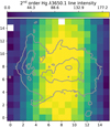 |
Fig. A.1. Intensity map of the second order UV Hg line at λ3650 Å, observed at 7300 Å, and used to obtain a UV flatfield. Hα contours of Mrk 71 are overplotted for orientation. |
In Fig. A.1 we show the intensity map of a 2nd order spectrum of the arc lamp line Hg λ3650 Å, which is used to obtain a UV flatfield for the second order [O II] λ3727 Å intensity map.
Appendix B: Continuum subtraction in narrowband filters
We use the mode method (Keenan et al. 2017) to estimate the continuum scaling factor for the Hα and Hβ HST filters. This method is similar to the skewness method of Hong et al. (2014), but uses the mode instead of the skewness, and performs equally well as other integrated scaling factor methods, as demonstrated in Micheva et al. (2018). This is an iterative method, based on evaluating the mode of the pixel histogram of the continuum-subtracted image as a function of different scaling factors μS. The mode of the pixel histogram of an image should decrease smoothly as the continuum is subtracted. Once the continuum becomes over-subtracted, the negative pixels will cause a rebinning of the pixel histogram, and a change of the relation between mode and μS. This manifests itself as a break in an otherwise smooth function. Since the break indicates the transition from undersubtraction to oversubtraction of the continuum, it marks the location of the optimal scaling factor. The mode of a histogram depends on the bin size used to make that histogram, and therefore one has to explore several bin sizes. Beyond a certain bin size, the behavior of the mode as a function of scaling factor converges to produce a break at the same position for all larger bin sizes. For each filter, the pixel histogram is computed over an area covering the entire galaxy. Identification of the best scaling factor is done graphically, as illustrated in Fig. B.1 for both Hα and Hβ continuum filters. In these plots of scaling factor μS vs. mode residual, the break occurs in a single location, and we easily identify μS = 0.1 for Hα continuum, and μS = 0.5 for Hβ continuum. Scaling factors below and above these values undersubtract and oversubtract the continuum, respectively. The solution seems quite stable, as indicated by the large range of bins producing the same break. In Fig. B.2 we show the resulting Hα/Hβ map, convolved to the seeing of our PMAS data, and resampled to the PMAS resolution of 1 arcsec per spaxel.
We use the same method to subtract the continuum in the HST F373N from the archive (PID 13041, PI: B. James), using the F336W filter from the same run. The corresponding scaling factor is μS = 0.75. The continuum-subtracted F373N image is used to calibrate the UV [O II] 3726 + 3729 second order emission lines in Sect. 2.2.
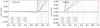 |
Fig. B.1. Continuum scaling factor μ as a function of the mode residual for the two HST filters F487N (Hβ, left panel) and F656N (Hα, right panel). The breaks in the two functions indicate a scaling factor of μS = 0.5 for Hβ and μS = 0.1 for Hα. |
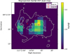 |
Fig. B.2. Seeing-convolved, reprojected reddening map from HST data. The theoretical Hα/Hβ = 2.86 at 104 K (Brocklehurst 1971), and so unphysically low values imply dust-free regions. Additionally, for display purposes spaxels with signal-to-noise ≲2 are set to the lowest shown value of 2.80. Hα contours are overplotted for orientation. |
All Tables
All Figures
|
Fig. 1. Top row: NGC 2366, with labeled major substructures and the PMAS field of view. Figure reproduced from Micheva et al. (2017b). Bottom row: continuum-subtracted Hα images from the HST (left panel) and PMAS (right panel). The positions of knots A and B are indicated with open circle and open square, respectively. HST Hα iso-intensity contours at 8.1 × 10⁻⁶, 1.3 × 10⁻⁶ and 1.9 × 10⁻⁷ erg s cm−2 Å arcsec−2, are overplotted on the PMAS image for orientation. The position angle of the HST field is rotated by ∼14 deg relative to the PMAS image. |
| In the text | |
|
Fig. 2. Sky-subtracted and flux-calibrated average spectrum from the PMAS data cube (left panel) of the region marked in the Hα intensity map (blue circles in right panel, at the center of each spaxel). All identified lines are labeled, including the UV [O II] second order spectrum. The sky emission at [O I] λλ6300, 6363 (gray dashed lines) could not be fully subtracted with the sky exposure. The y-axis is truncated in order to better show weak lines like [O II] λλ7320, 7330. Vignetting affects the regions λ ≲ 6175 Å and λ ≳ 7300 Å at the edges of the detector (columns x = 0 and x = 15). |
| In the text | |
|
Fig. 3. (A) Instrumental broadening for 26 HgNe arc lines (filled circles), here for representation purposes obtained by stacking the spectra along columns in (B). The data points and the ID of the column that produced them have the same color-coding. The colored solid lines are a sixth order polynomial fit, used to interpolate the resolving power at the desired wavelength. (B): An example resolving power map close to Hα. The x-axis shows the column ID, color-coded as in (A). |
| In the text | |
|
Fig. 4. (A): Hα radial velocity distribution around the luminosity-weighted average velocity zero-point of 95.34 km s−1. HST Hα countours are overplotted in gray solid lines, with the outer most (faintest) contour tracing the 1.9 × 10⁻⁷ erg s cm−2 Å arcsec−2 iso-intensity level. (B): Hα velocity dispersion, corrected only for instrumental broadening. Only spaxels with S/N ≥ 10 are shown. The gray spaxels at positions (0,14) and (8,15) are dead fibers. |
| In the text | |
|
Fig. 5. Left column: Averaged spectra for different spatial regions, in arbitrary flux density units, scaled to match in Hα equivalent width. The continuum has been subtracted from both the blue and orange spectra, enabling comparison between panels in different rows. Middle column: Intensity-velocity dispersion diagrams for Hα. The horizontal line in each panel is 〈σm〉. Markers are color-coded by the spatial location of their corresponding spaxels, shown in the right column. We note that the y-axis values are di played on the right-hand side. Right column: Spatial maps of Hα, identifying the different regions. North is up, east is to the left. |
| In the text | |
|
Fig. 6. (A): Electron temperature log10Te[K]. Knots A (green open circle) and B (green open square), as well as Hα contours are overplotted for orientation. Numbers indicate relative error, with “0.1” corresponding to 0.1 ≤ δTe/Te < 0.2, etc. Spaxels with no numbers have δTe/Te < 0.1. (B): Electron density log10ne[cm−3]; same legend as in (A). Both Te and ne are obtained with pyneb. |
| In the text | |
|
Fig. 7. (A): Speed of sound cS. Knots A (open circle) and B (open square) are given for orientation. (B): Thermal broadening. (C) “True” velocity dispersion, corrected for both instrumental and thermal broadening. (D) Mach number ℳ map, with strictly hypersonic regions (ℳ ≥ 5.0) marked with “x”. At knot B, ℳ = 4.63. |
| In the text | |
|
Fig. 8. Velocity dispersion, corrected only for instrumental broadening, with overplotted dust contours. The cone of 2× the Mach angle of downstream propagation of perturbations is also plotted for the Mach number at knot B (open square), ℳ = 4.63. The extinction outside of the plotted contours is negligible, see the reddening map in Fig. B.2. |
| In the text | |
|
Fig. 9. High-resolution runs of the SILCC simulations (Girichidis et al. 2018). The white rectangle indicates the area comparable to our observations. Top row: edge-on projection of the galactic disk, the bottom panel one the face-on view. See Sect. 5 for details. |
| In the text | |
|
Fig. 10. Same as Fig. 9 but showing only the column density for the three considered gas phases. The white rectangle marks the region comparable to the observation. The column density range for the ionized gas is much smaller than for the other two components. The bright spot in the ionized column corresponds to a recently exploded supernova. |
| In the text | |
|
Fig. 11. west region average-stacked observed spectrum (thick gray line) around Hα, compared to (A) average-stacked single Gaussian models (orange line) and individual observed spectra (thin gray lines); (B) Empirical LSF (orange line) and LSF-convolved single Gaussian of various widths (blue lines); (C) composite model (orange line) of a broad Gaussian (green line) added to an LSF-convolved narrow Gaussian of width σ = 0.7 Å. |
| In the text | |
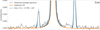 |
Fig. 12. Same as Fig. 11b but for the east region. No broad component is detected. |
| In the text | |
|
Fig. 13. Left panel: Hα radial velocity as a function of the radial velocity in lines tracing low-ionization ([N II], [S II]) and high-ionization gas (He I, [Ar III]). The points are color-coded by S/N. The 1:1 Hα velocity line (solid gray), with ±5 (dashed) and ±10 km s−1 (dotted) lines, are plotted for orientation. Only spaxels with S/N ≥ 15 or within the overplotted contours in the right panel are shown. Right panel: spatial distribution of the spaxels, color-coded by S/N. |
| In the text | |
|
Fig. A.1. Intensity map of the second order UV Hg line at λ3650 Å, observed at 7300 Å, and used to obtain a UV flatfield. Hα contours of Mrk 71 are overplotted for orientation. |
| In the text | |
|
Fig. B.1. Continuum scaling factor μ as a function of the mode residual for the two HST filters F487N (Hβ, left panel) and F656N (Hα, right panel). The breaks in the two functions indicate a scaling factor of μS = 0.5 for Hβ and μS = 0.1 for Hα. |
| In the text | |
|
Fig. B.2. Seeing-convolved, reprojected reddening map from HST data. The theoretical Hα/Hβ = 2.86 at 104 K (Brocklehurst 1971), and so unphysically low values imply dust-free regions. Additionally, for display purposes spaxels with signal-to-noise ≲2 are set to the lowest shown value of 2.80. Hα contours are overplotted for orientation. |
| In the text | |
Current usage metrics show cumulative count of Article Views (full-text article views including HTML views, PDF and ePub downloads, according to the available data) and Abstracts Views on Vision4Press platform.
Data correspond to usage on the plateform after 2015. The current usage metrics is available 48-96 hours after online publication and is updated daily on week days.
Initial download of the metrics may take a while.