| Issue |
A&A
Volume 623, March 2019
|
|
|---|---|---|
| Article Number | A146 | |
| Number of page(s) | 17 | |
| Section | Stellar structure and evolution | |
| DOI | https://doi.org/10.1051/0004-6361/201834703 | |
| Published online | 22 March 2019 | |
Probing Polaris’ puzzling radial velocity signals
Pulsational (in-)stability, orbital motion, and bisector variations⋆
1
European Southern Observatory, Karl-Schwarzschild-Str. 2, 85748 Garching b. München, Germany
e-mail: This email address is being protected from spambots. You need JavaScript enabled to view it.
2
Département d’Astronomie, Université de Genève, 51 Ch. des Maillettes, 1290 Sauverny, Switzerland
Received:
22
November
2018
Accepted:
18
February
2019
Abstract
We investigate temporally changing variability amplitudes and the multi-periodicity of the type-I Cepheid Polaris using 161 high-precision radial velocity (RV) and bisector inverse span (BIS) measurements based on optical spectra recorded using Hermes at the 1.2 m Flemish Mercator telescope on La Palma, Canary Islands, Spain. Using an empirical template fitting method, we show that Polaris’ RV amplitude has been stable to within ∼30 m s−1 between September 2011 and November 2018. We apply the template fitting method to publicly accessible, homogeneous RV data sets from the literature and provide an updated solution of Polaris’ eccentric 29.3 yr orbit. While the inferred pulsation-induced RV amplitudes differ among individual data sets, we find no evidence for time-variable RV amplitudes in any of the separately considered, homogeneous data sets. Additionally, we find that increasing photometric amplitudes determined using SMEI photometry are likely spurious detections due to as yet ill-understood systematic effects of instrumental origin. Given this confusing situation, further analysis of high-quality homogeneous data sets with well-understood systematics is required to confidently establish whether Polaris’ variability amplitude is subject to change over time. We confirm periodic bisector variability periods of 3.97 d and 40.22 d using Hermes BIS measurements and identify a third signal at a period of 60.17 d. Although the 60.17 d signal dominates the BIS periodogram, we caution that this signal may not be independent of the 40.22 d signal. Finally, we show that the 40.22 d signal cannot be explained by stellar rotation. Further long-term, high-quality spectroscopic monitoring is required to unravel the complete set of Polaris’ periodic signals, which has the potential to provide unprecedented insights into the evolution of Cepheid variables.
Key words: stars: individual: Polaris / stars: variables: Cepheids / binaries: spectroscopic / binaries: visual / stars: oscillations / techniques: radial velocities
Full Table A.1 is only available at the CDS via anonymous ftp to cdsarc.u-strasbg.fr (130.79.128.5) or via http://cdsarc.u-strasbg.fr/viz-bin/qcat?J/A+A/623/A146
ESO fellow.
© ESO 2019
1. Introduction
The North Star, Polaris1, is a celebrity among type-I Cepheid variable stars (henceforth: Cepheids) thanks to its proximity, uncertain physical properties, and plentiful literature concerning its puzzling variability properties. Being the closest Cepheid to the Sun, one might expect Polaris to have a prototypical role in the understanding of Cepheids in general, which are both important stellar laboratories and accurate cosmic yardsticks. In particular the application of Cepheids as standard candles for determining the value of the Hubble-Lemaître constant with high accuracy (Riess et al. 2018, 2016) provides a strong motivation for achieving a solid understanding of their astrophysical properties. Yet, Polaris continues to defy a detailed description, with several recent articles struggling to explain its mass, radius, age, and other properties (cf. Bond et al. 2018; Anderson 2018a; Evans et al. 2018). Most recently, Usenko et al. (2018) have refueled previous discussions on the stability of Polaris’ variability, which may be the key to explaining this uncomfortable situation.
Polaris’ weak photometric variability was first noticed in the mid 19th century (Seidel 1852) and was only fully confirmed in the early 20th century (Hertzsprung 1911; King 1912; Pannekoek 1913). Early radial velocity (RV) observations using the Mills spectrograph at Lick Observatory (Campbell 1898) revealed RV variability on two timescales, leading Campbell (1899) to conclude that Polaris “is at least a triple system2”. Thirty years later Moore (1929) determined an orbital period, Porb, of 29 years.
Roemer (1965) confirmed this orbit and noted irregularity in the periodicity of the RV variations and adopted different photometrically determined pulsation periods, Ppuls, for different epochs of RV measurements. Indeed, the rate of period change is exceptionally high for Polaris (Turner et al. 2005, Ṗ ∼ 4.5 s yr−1), which implies a first crossing the classical instability strip, i.e., that Polaris populates the Hertzsprung gap and has not yet undergone the first dredge-up event (Anderson et al. 2016a). Turner et al. (2005) further noticed an abrupt change to Ppuls between 1963 and 1966, which cannot be explained using the standard interpretation of secular evolution.
Arellano Ferro (1983) reported first indications of a time-variable amplitude, suggesting that Polaris was about to exit the instability strip. Despite focusing on photometric observations, Arellano Ferro also made brief reference to a significant decrease in RV amplitude between the Lick velocities (2K ∼ 6 km s−1) and newer RVs measured (2K ∼ 2 km s−1) at the David Dunlap Observatory (DDO; cf. also Kamper et al. 1984). This report sparked much interest in Polaris, leading to confirmations of a decreased RV amplitude and predictions that Polaris would cease pulsating in the mid 1990s (Dinshaw et al. 1989; Fernie et al. 1993). However, Polaris’ RV amplitude appeared to stabilize by late 1997 (Kamper & Fernie 1998; Hatzes & Cochran 2000) and even showed a slow but noticeable increase in between 2004 and 2007 (Lee et al. 2008; Bruntt et al. 2008). Most recently, Usenko et al. (2018) reported a significantly higher RV amplitude around 3.8 − 2.8 km s−1, which they interpreted as a sign for possibly cyclic amplitude variations. In this context it is worth pointing out that Polaris’ pulsational RV amplitude is abnormally low, even among Cepheids pulsating in the first overtone. To wit, Klagyivik & Szabados (2009) determined the average peak-to-peak amplitude of single (binary) FO Cepheids in the Milky Way to be 15.8 ± 4.1 km s−1 (18.2 ± 4.7 km s−1), with V1726 Cyg having the lowest amplitude of 8.5 km s−1 (not counting Polaris).
Polaris’ variable photometric amplitudes have also been studied in detail following the initial discovery of amplitude variations by Arellano Ferro (1983). For example, Spreckley & Stevens (2008) and Bruntt et al. (2008) independently analyzed photometric observations by the Solar Mass Ejection Imager (SMEI) instrument on board the Coriolis space craft and concluded that the photometric amplitude of Polaris showed a significant increase between 2004 and 2007, thus creating an important link between photometric amplitude growth and the contemporaneous reports of growing RV amplitudes.
Additional periodic signals were reported by Dinshaw et al. (1989, 45.3 d), Kamper & Fernie (1998, 34.3 d), Hatzes & Cochran (2000, 17.03 and 40.2d; henceforth: HC00), Lee et al. (2008, 119 d), and Bruntt et al. (2008, 2 − 6d; henceforth: B+08). However, none of these studies confirmed any previously reported periodicities (not even using contemporaneous data sets), and B+08 concluded that any detections of signals on periods longer than 6 d had been spurious and caused by instrumental drifts or complicated spectral windows.
Meanwhile, Cepheid light curves in general have been shown to be much more complex than previously thought (e.g. Poleski 2008; Evans et al. 2015; Poretti et al. 2015; Derekas et al. 2017; Smolec 2017; Süveges & Anderson 2018) and high-precision RV observations have revealed both cycle-to-cycle and long-term modulations (Anderson 2014). Unfortunately, the relation between photometric and velocimetric variability modulations remains unclear due to a combination of observational selection effects, particularly involving brightness limits, available reference stars, and modulation timescales. Among the best-studied cases is the long-period Cepheid ℓ Car (Ppuls = 35.5 d) that exhibits cycle-to-cycle RV curve modulations as well as temporal variations of its maximum angular diameter. Intriguingly, a contemporaneous study using optical/near infrared interferometric and optical RV data showed that both types of signals were modulated, yet that there was no direct correspondence between the two modulation signals (Anderson et al. 2016b). Hence, photospheric motions (traced by photometry and interferometry) and gas motions (traced by spectral lines) appear to be affected by different physical processes responsible for the modulations.
As the above shows, the literature on Polaris contains many conflicting reports concerning amplitude variations, some of which are based on highly inhomogeneous data sets, as well as the presence of additional periodic signals. A reconsideration of the (in-)stability of Polaris’ RV variability is thus in order, in particular in light of the recent reports of a renewed decline in RV amplitude.
This paper is structured as follows. Section 2 presents a new set of highly precise RVs of Polaris (Sect. 2.1) as well as an empirical template fitting method (Sect. 2.2) used to investigate long-term RV variations. Section 3 presents the results of applying the template fitting method to Hermes RVs (Sect. 3.1) and publicly accessible data sets from the literature (Sect. 3.2). Section 3.3 provides an updated orbital solution for the 29-year orbit of the Polaris Aa-Ab system based on the results from the template fitting method. The discussion in Sect. 4 focuses on reliability of reported amplitude variations and additional periodicities. Specifically, Sect. 4.1 discusses the impact of data inhomogeneity on RV amplitudes, Sect. 4.2 investigates amplitude variations in the full SMEI data set, Sect. 4.3 considers additional periodic signals revealed by line bisector measurements, and Sect. 4.4 aims to consolidate the information from previous and new findings to achieve a clearer picture of Polaris. The final section Sect. 5 summarizes the results and conclusions.
2. Observational data and analysis
2.1. Hermes observations
Polaris was observed using the high-resolution Echelle spectrograph Hermes as part of a large observing program dedicated to high-precision velocimetry of classical Cepheids (Anderson et al., in prep.). Hermes features a resolving power of R ∼ 85 000 and is mounted to the Flemish 1.2 m Mercator telescope located on the Roque de los Muchachos Observatory on La Palma, Canary Island, Spain (Raskin et al. 2011). All observations were made using the high-resolution fiber to achieve the best throughput and spectral resolution. The data were reduced using the dedicated reduction pipeline that carries out standard processing steps such as flat-fielding, bias corrections, order extraction, and cosmic clipping. The measurements are provided in Table A.1.
The 161 observations presented here were gathered between 11 September 2011 and 20 November 2018, mostly during observing runs of 9–11 nights duration. Occasionally, observations could be secured in between the regular observing runs through time exchanges with other groups. RVs are determined using the cross-correlation method (Baranne et al. 1996; Pepe et al. 2002). The measured RV is defined as the center of a Gaussian profile fitted to a cross-correlation function (CCF) computed using the spectral orders 55 − 74 and a numerical mask that includes the position and relative strength of approximately 1130 metallic absorption lines found in a G2 star of Solar metallicity. The median signal-to-noise (S/N) of the spectra in this wavelength range is 230. Further details can be found in Anderson et al. (2015) and will be provided as part of the full Cepheid RV catalog (Anderson et al., in prep.), including derived velocities of RV standard stars (Udry et al. 1999). Figure 1 shows the full Hermes RV time series presented here.
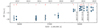 |
Fig. 1. Hermes radial velocity curve of Polaris as a function of observing date. The short term scatter is due to the ∼4 d pulsation, the long-term variations reveal the orbital motion whose pericenter passage occurred in late 2016. |
Several steps were taken to achieve maximum short-term RV precision and track long-term RV stability. To ensure short-term precision, we have continuously monitored the nightly evolution of the ambient pressure, and re-calibrated the wavelength solution whenever pressure variations exceeded ∼0.4 − 0.5 mbar, thereby reducing intra-night variations of the instrument’s RV zeropoint. Additionally, we compute RV drift corrections due to pressure changes following Anderson (2013, Ch. 2.3). This combined procedure achieves a short-term instrumental stability of approximately 10 − 15 m s−1 over the duration of one observing run (10 nights).
The long-term stability was monitored by means of RV standard stars. A preliminary analysis of the standard star monitoring indicates a very stable RV zeropoint (better than 20 m s−1) from 2011 to 2017 with a possible increase of about 50–70 m s−1 after 2017. The investigation of this offset is ongoing. Long-term RV zero-point variations to first order lead to changes in the mean RV at a given epoch; a spectral type-dependence of any zero-point offsets can lead to phase-dependent changes in the derived RV. However, such changes lead to (in this case) negligible second order effects on the order of a few m s−1.
2.2. RV template fitting
We determine temporal variations of the pulsation-averaged velocity, vγ, using a self-consistent empirical template fitting approach. The method was presented in detail by Anderson et al. (2016c), where it was used to investigate orbital motion in long-period Cepheids. In principle, the template fitting method can simultaneously solve for Ppuls variations. However, the short time span of the individual observing epochs of typically 5 − 10 d (1 − 2.5 pulsation cycles), with one exception of 35 d, is too short to precisely constrain Ppuls for each epoch. After experimenting with time-variable Ppuls at first, we found employing a fixed value for Ppuls to be a sounder approach. To this end, we first subtract an orbital model3 from the RV time series and then determine the peak of highest power in a Lomb-Scargle periodogram (Lomb 1976; Scargle 1982) computed on the residuals using astropy4. The uncertainty on Ppuls can be determined from a χ2 distribution computed for a dense grid of input periods, so that  . However, in the case of Polaris,
  due to relatively large residual scatter (RMS ∼ 223 m s−1) after the orbit removal. We therefore adopt
  as the 1σ confidence level and find Ppuls = 3.97198 ± 0.00004 d at Epoch 2456553.62553 in 2σ agreement with 3.97209 ± 0.00004 d derived on SMEI data between 2003 − 2007 (Spreckley & Stevens 2008).
We adopt a reference epoch to define the pulsation template. This reference epoch is chosen from the full time series data such that good phase coverage is achieved over a relatively short timescale in order to avoid noise from period or amplitude fluctuations as well as orbital motion. The template to be applied to all other epochs is then defined by the best-fit Fourier series model (we find that two harmonics are best-suited for Hermes data) of this reference data set using Ppuls = 3.97198 d determined above. The full RV time series is then sub-divided into epochs of short duration (cf. alphabetic labels in Fig. 1) and the reference pulsation model is fitted to each epoch using a least-squares routine that varies offsets in vγ and determines a phase offset such that the pulsation phase ϕ ≡ 0 at minimum RV.
The most suitable reference epoch was epoch (c) in mid 2013, which is near the minimum RV of the 29-year orbit. The reference epoch consists of 26 measurements secured over the course of 9 nights and is shown in Fig. 2. The peak-to-peak amplitude is 3.526 ± 0.006 km s−1 and Table 1 lists the Fourier coefficients derived. We find that a linear trend  d−1 is needed to account for orbital motion and possible additional RV variations (cf. Sect. 4.3) during the reference epoch. We therefore introduce an additional fit parameter,
  , in the template fitting routine in order to account for trends acting on the timescale of an observing epoch.
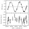 |
Fig. 2. RVs of Polaris at the reference epoch (c) chosen for its densest phase coverage over a short timescale. Top panel: Hermes data as a function of Barycentric Julian Date with the overplotted model consisting of the reference Fourier series model and a slow linear term of 9 ± 1 m s−1 d−1. Bottom panel: residuals of the fit, with an RMS of 13 m s−1. The grayscale traces observing date as is done for the template fits below. |
Fit coefficients determined for the reference epoch per data set.
The reference epoch’s reduced χ2 is unity for an assumed short-term precision of approximately 13 m s−1. We therefore adopt 15 m s−1 as the error of the Hermes RVs. This value agrees well with the short-term RV precision determined using RV standard stars, indicating that the zero-point stability is the dominant uncertainty on these measurements as previously found for δ Cep (Anderson et al. 2015). While 15 m s−1 is a reasonable estimate of the short-term RV precision, longer-term zero-point variations affect vγ at the level of up to 50 − 70 m s−1 over the 7 year time span. Therefore, the larger error of 70 m s−1 is adopted for determining the orbit (Sect. 3.3).
3. Results
3.1. RV template fitting applied to Hermes data
The RV template fitting procedure (Sect. 2.2) solves for three parameters: vγ, Δϕ, and  using the fixed set of Fourier coefficients determined from the reference epoch. Since the amplitude of the fitted model is constant, any temporal variations of Polaris’ RV amplitude would lead to increased fit residuals, in particular near the minimum and maximum of the pulsation-induced RV variability. Assuming perfect phase coverage, a linear dependence of RV curve amplitude on time would tend to introduce a dependence of residual scatter on time. Conversely, a constant scatter in the fit residuals indicates stable RV variability.
The results from the template fitting applied to Hermes RVs are illustrated in Fig. 3 and listed in Table 2, including the values of vγ,  and each epoch’s fit RMS. Each panel in Fig. 3 shows the RV data and template fit for one epoch as labeled in Fig. 1. The data in each panel are color-coded to trace the observing date during that epoch. Figure 3 readily shows the long-term orbital motion that slowly modulates the per-epoch average of the RV curve. Residuals are shown underneath each panel. The mean per-epoch RMS is 28 m s−1, with a maximum of 56 m s−1 during epochs a and e. Epoch e is close to pericenter passage and the most sensitive to orbital motion within the duration of the epoch’s observations. Figure 4 illustrates the template fit residuals whose minimum and maximum values are −91 m s−1 and +119 m s−1 (both in epoch e), with an overall mean residual of 31 m s−1. By construction, a very close fit is obtained for the reference epoch (c). Less densely sampled epochs can exhibit larger scatter due to variations or fluctuations of Ppuls as well as potentially real variations in the RV curve shape. However, Figs. 3 and 4 clearly demonstrate that the pulsational RV amplitude of Polaris was stable at the level of ∼30 m s−1 over the entire duration of the observing program (2011–2018). Specifically, they exclude the large, km s−1-level amplitude variations between 2017–2018 (traced by epochs g through j) reported by Usenko et al. (2018).
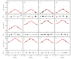 |
Fig. 3. Per-epoch template fits to Hermes RV data. In each panel, a gray scale is applied to distinguish the observing data internal to the given epoch, i.e., the gray scale runs from white to black among the measurements of that epoch. For each epoch, we show the Hermes data phase-folded and zero-phase shifted as determined from the template fit. The red solid curve in each panel is the pulsation model (cf. Fig. 2), shifted to the vγ of that epoch. Fit residuals are shown underneath each template fit, and a grayscale traces observing date in each epoch (white to black). |
Results from the template fitting analysis applied to RV data of Polaris from Hermes, Kamper (1996), and Gorynya et al. (1992).
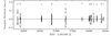 |
Fig. 4. Hermes RV template fit residuals as a function of observing date. The highest scatter is found in epoch (e), which is near pericenter passage and thus the most sensitive to orbital motion. |
3.2. RV template fits applied to literature data
We apply the RV template fitting method to literature RVs in order to test RV curve stability for separate, homogeneous data sets and to determine the temporal variation of vγ. To this end, we employ: RVs measured by Kamper (1996, henceforth: K96) using high-dispersion (8 mm Å−1) photographic DDO spectra (K96-08 RVs), RVs measured by K96 using the DDO spectrograph following the installation of a 1024 × 1024 Thomson CCD (K96-CE RVs), and RVs determined by Gorynya et al. (1992) using the Moscow Coravel-type correlation spectrometer (Tokovinin 1987) (Gorynya RVs). The K96-08 and K96-CE data sets are the two largest subsets of the data published by K96. As Fig. 5 shows, various interventions at the telescope led to noticeable zero-point changes, which were occasionally accompanied by significant spurious zero-point fluctuations, e.g. following the installation of the CCD. Specifically, K96 noted that “observations were standardized” only after the “surprising decrease in pulsational amplitude” by Arellano Ferro (1983). The K96-CE data are internally more precise on short timescales than the K96-08 data, although the template fits indicate calibration issues in the first season after the CCD camera had been installed at the spectrograph. Unfortunately, the zero-point seems to vary significantly between each observational epoch (cf. Fig. 5, blue squares), so that the inferred values of vγ are not useful for determining the orbit.
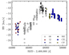 |
Fig. 5. Radial velocity data from Kamper (1996) measured at DDO. Different symbols and colors are used to distinguish data measured using different instrumental setups. Labels “08”, “12”, and “16” refer to photographic of different dispersions (in mm Å−1). “RE” refers to measurements taken using a Reticon detector, “CF” to ones using a fiber link, and “CE” to observations made using a CCD. Instrumental zero-point variations related to these interventions and associated calibration issues are readily apparent, especially following the peak of the orbital RV variation near HJD 2 445 750. |
The Gorynya RVs are relatively few and noisy compared to the K96 data sets. However, the larger catalog of Cepheid RVs published by Gorynya et al. (1992, 1996, 1998) provides a unique and fairly homogeneous basis for comparing Cepheid RVs over timescales of several decades. Based on a preliminary analysis of Cepheids observed as part of our ongoing program (Anderson et al., in prep.), the Gorynya data generally agree very well with RVs determined using Hermes. For instance, we determine peak-to-peak RV amplitudes of 27.70 km s−1 vs. 27.73 km s−1 for ζ Gem (using 5 harmonics), and 17.11 km s−1 vs. 17.24 km s−1 for EU Tau based on Hermes and Gorynya data, respectively. Other RV data sets previously discussed in the literature were either not publicly available, or were not listed on an absolute scale so that the orbital motion cannot be inferred directly.
Table 1 lists the Fourier coefficients of the sinusoidal reference curves and Table 2 lists the results of the template fits applied to literature RVs. Given the lower precision of the literature data, we do not solve for any linear trends  as was the case for the Hermes data. Appendix B illustrates the template fit results of the K96-08 and K96-CE data. None of the three literature data sets analyzed here exhibit noticeable RV amplitude differences exceeding a few hundred m s−1, i.e., at the level of the precision of the data. Instead, the reference epochs of the three literature data sets yield stable peak-to-peak RV amplitudes that agree to within their uncertainties: 1.51 ± 0.21 km s−1 (K96-08), 1.63 ± 0.02 km s−1 (K96-CE), and 1.2 ± 0.4 km s−1 (Gorynya). The aforementioned general agreement between a large number of Cepheid RV amplitudes based on Gorynya’s data and Hermes would tend to support the interpretation that the pulsational RV variability of Polaris has changed over time. Specifically, this would imply that the RV amplitude more than doubled between 1995 and 2011, while homogeneous data sets recorded both before and after this period exhibit no significant changes. However, we notice that many of the Gorynya RVs exhibit scatter of up to 1 − 2 km s−1 among measurements obtained in rapid succession (on timescales of minutes), which could point to a problem with these particular measurements.
For comparison, Lee et al. (2008) reported non-monotonous variations in RV amplitude with 2K = 2.2, 2.1, and 2.4 km s−1 in 2005, 2006, and 2007, whereas B+08 (cf. their Fig. 4) reported a rather monotonous increase in amplitude from 2K ∼ 1.9 to 2.1 and 2.3 km s−1 during the same years. B+08 derived a linear relation for the RV amplitude of ARV(t)=(0.90 ± 0.01)+(1.45 ± 0.15)×10−4(t − t0) km s−1, where t0 = 2 453 000. Converting this relation to peak-to-peak amplitudes (2K) and projecting it to the first epoch of Hermes measurements would imply 2K ∼ 2.62 km s−1, which is significantly less than the 2K = 3.5 km s−1 observed using Hermes, cf. Table 2. Taken at face value, this implies that the RV amplitude has increased much faster between 2007 and 2011 than between 2004 and 2007, and that it has since remained nearly constant. Calculating the amplitude expected for the last K96-CE epoch using this linear relation yields 2K ∼ 0.81 km s−1, which is much lower than the observed 1.6 km s−1. Hence, the comparison of results based on data sets with differing systematics suggests that Polaris’ RV amplitude may vary significantly in a non-linear fashion over timescales of up to a few years. Given the strong interest in Polaris, it is somewhat surprising and very unfortunate that there exists no homogeneous data set that unambiguously demonstrates the fast and non-linear RV amplitude variations implied by this comparison of literature amplitudes, especially since it is difficult to distinguish between (small) amplitude changes caused by astrophysical effects and non-astrophysical systematics related to drifting RV zero-points, inhomogeneous data sets, or incompatible RV measurement definitions, cf. Sect. 4.1.
3.3. An updated orbital solution for Polaris Aa-Ab
We determine an updated orbital solution for the Polaris Aa-Ab system using the results from the RV template fits5 performed in Sects. 3.1 and 3.2. To measure the orbit accurately, it is important to account for RV zero-point differences among the inhomogeneous literature. Combining all recent data sources is unfortunately not advisable due to a combination of insufficient knowledge of standard star velocities, unstable zero-points, and literature RVs having occasionally been corrected for orbital motion. Fortunately, both the Hermes data and the K96-08 data span the pericenter passage of the eccentric orbit as well as the extremes of the orbital RV curve. Correcting for the mid-point difference in the orbital RV curves, we find an approximate zero-point offset of −0.7 km s−1 between K96-08 and Hermes. Adding 0.7 km s−1 to the K96-08 vγ values, we determine best-fit orbital solutions for a range of small zero-point shifts near this value. The solution with the minimum χ2 is adopted as the correct zero-point shift and yields −0.63 km s−1. The Gorynya RVs are not used in the orbital fit, since they span a short a time interval (98 d) and exhibit large short-term (timescale of minutes) scatter on the order of 1 km s−1.
We fit a Keplerian model to the zero-point corrected vγ time series using Porb = 29.6 yr (K96) as the starting value and determine the solution listed in Table 3. Figure 6 illustrates the result obtained, which for the most part agrees to within the uncertainties with the solution by K96. Besides a small difference in Porb, the principal difference between the two solutions is the center-of-mass velocity of the binary system, which directly depends on the instrumental zero-point. The slightly larger uncertainties of our result are primarily due to the higher precision of the RV data, which are very sensitive to imperfections in the removal of the pulsation model. These imperfections lead to an elevated  , which linearly affects the reported fit uncertainties derived from the diagonal elements of the fit covariance matrix.
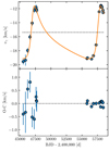 |
Fig. 6. Orbital solution based on the RV template fitting procedure applied to data from Hermes and the high-dispersion photographic RVs from Kamper (1996, K96-08 RVs). The K96-08 RVs have been zero-point corrected by 0.63 km s−1, cf. Sect. 3.3. |
Despite the slightly larger uncertainties, our new orbital solution benefits from a much higher degree of data homogeneity than previous solutions as well as the overall high accuracy of the Hermes RV zero-point. This is particularly important when considering the center-of-mass velocity of the Polaris Aa-Ab system (−15.387 ± 0.040 km s−1), which agrees to within 1σ with Polaris B’s RV of −22.25 ± 8.11 km s−1 as reported in Gaia DR2 (Gaia Collaboration 2018; Cropper et al. 2018; Katz et al. 2019).
4. Discussion
4.1. Data inhomogeneity and amplitude variations
The first studies of Polaris’ RV signals employed photographic spectra taken with the same spectrograph. Roemer (1965) explained that observations between 1896 and January 1903 were centered on Hγ (“old” Mills setup), whereas observations between summer 1903 and the last observation in 1958 were centered near 4500 Å (“new” Mills setup). Telescope flexure corrections of up to ±0.3 km s−1 were included after 1920. Unfortunately, the original publications do not specify which spectral lines were measured, nor how RV was defined, e.g. whether line barycenters, line cores, or other ways of measuring line positions were used. It is also not possible to tell whether measurements were performed on multiple lines and how such measurements were averaged. For instance, K96 notes that DDO velocities were based on a cross-correlation, although it is not specified which lines were combined in this cross-correlation. This creates an issue for comparing literature amplitudes among one another, because the hydrodynamics of a Cepheid’s atmosphere introduce phase shifts and amplitude differences between different transitions formed at different heights (e.g. Grenfell & Wallerstein 1969; Butler 1993; Petterson et al. 2005; Nardetto et al. 2007; Anderson 2016).
The greatly extended wavelength ranges offered by modern Echelle spectrographs connected to CCD detectors have potentially introduced a systematic offset for RV amplitudes of pulsating stars compared to amplitudes measured based on more restricted wavelength intervals. Amplitude differences among inhomogeneous RV data sets may therefore to some extent be explained by different weighting of differentially moving atmospheric layers. In extreme cases, amplitude differences between spectral lines or measurement definitions can exceed a few km s−1, cf. Anderson (2018b) for a recent review. Since the 1980s, researchers were faced with rapidly evolving instrumental technology while RV measurements became more and more common with time. This has lead to a highly inhomogeneous data set of relatively short time intervals as can be seen from the data presented by K96 as shown Fig. 5. To what extent such layer-averaging effects can introduce amplitude variations for Polaris’ generally low amplitude (cf. Kovacs et al. 1990; Anderson et al. 2016c) will be investigated in detail in future work.
The following RV amplitudes (K denotes semi-amplitude of a sinusoid) were previously reported using a variety of spectrographs covering different wavelength ranges: 2K = 1.50 ± 0.08 km s−1 in 1987–1988 (Dinshaw et al. 1989, λ4220 − 4700 Å); 2K ∼ 1.53 km s−1 in 1994 (Hatzes & Cochran 2000, Δλ ∼ 23.6 Å centered on λ5520 Å and using an iodine absorption cell); 2K ∼ 1.6 km s−1 in 1994–1997 (Kamper & Fernie 1998, wavelength center changed to λ6290 Å to enable telluric line corrections); 2K ∼ 2.1 − 2.4 km s−1 between 2004 and 2007 (Lee et al. 2008, typically 160–180 lines over an unclear spectral range, between λ3600 − 10 500 Å, using an iodine absorption cell); 2K ∼ 2 km s−1 with a possible time-dependence from late 2003 to late 2007 (Bruntt et al. 2008, based on 74 strong mostly FeI lines between λ5000 − 7100 Å). Given the issue of inhomogeneity, the cleanest evidence for RV amplitude variations is the contemporaneous detection of RV amplitude variations (cf. Sect. 3.2) using independent data sets by Lee et al. (2008) and B+08. Although B+08 provide a linear relation for the RV amplitude increase, their Fig. 4 may indicate non-linearity in these RV amplitude changes. However, it is suspicious that such non-linearities would only occur near both ends of the time series. Moreover, although the results from the template fitting routine applied in Sect. 3.2 confirm individually different RV amplitudes based on different data sets, we find no evidence for amplitude variations within any given homogeneous data set. Finally, the new Hermes RVs exclude significant (> 30 m s−1) amplitude variations over the course of 7 years, cf. Sect. 3.1.
To summarize, amplitude differences of 1 − 2 km s−1 have been noted among different literature data sets spanning several decades. Unfortunately, the most significant RV amplitude changes seem to have occurred in between the various studies, i.e., when no RV observations were carried out. The cleanest examples of varying RV amplitudes on the order of 200 − 300 m s−1 were provided by Lee et al. (2008) and B+08, although these relatively weak variations do not explain the extent of the long-term variations as a whole. Hence, even more significant amplitude variations would have had to occur on relatively short timescales of at most a few years in order to explain the observed trends. However, the fact that none of the more precise, long-term RV programs–including K96-CE, B+08, Lee et al. (2008), and the Hermes data–reveal such fast and significant amplitude variations casts some doubt on the assumed astrophysical origin of the reported amplitude differences.
4.2. Anti-correlation between amplitude and mean magnitude trends in SMEI
The Solar Mass Ejection Imager (SMEI) on-board the Coriolis spacecraft monitored nearly every point in the sky every 102 minutes between January 2003 and late September 2011 (Eyles et al. 2003). SMEI thus provided extremely dense time-series photometry of very bright stars down to approximately R ∼ 10 mag (Buffington et al. 2006). After about 3–4 years of observations, SMEI data were used to report on Polaris’ increasing amplitude6 of ∼1.87 ± 0.09 mmag yr−1 (B+08) and 1.39 ± 0.12 mmag yr−1 (Spreckley & Stevens 2008). These detections have played a crucial role in establishing confidence in contemporaneous RV amplitude variations reported in the literature.
SMEI continued observing Polaris until 17 days after our Hermes observations began. To the best of our knowledge, the full SMEI Polaris data have not been presented in a refereed publication. However, Švanda & Harmanec (2017) briefly describe results from a wavelet analysis applied to the full SMEI time series, confirming the previously reported amplitude growth at a rate of 2.40 ± 0.08 mmag yr−1. Švanda & Harmanec (2017) further note that no significant variations of the dominant pulsation period are found, with Ṗ = 35 ± 28 s yr−1. For comparison, Berdnikov et al. (2010) reported detections of period fluctuations in four bright Cepheids observed by SMEI.
The 8.65 yr baseline of SMEI observations offers a unique opportunity to bridge the gap between the RV observations reported B+08 and the new Hermes measurements since photometric amplitudes generally scale with RV amplitudes (e.g. Klagyivik & Szabados 2009). To this end, we retrieved the full time series of Polaris (spanning January 2003 to 28 September 2011) from the online SMEI archive7. We perform a conservative and rudimentary data cleaning to remove artifacts of obviously instrumental origin as follows. First, we compute residuals of a linear fit to the time series in order to be insensitive to an obvious temporal increase in mean magnitude seen for most stars observed with SMEI. Second, we reject data points lying farther than 0.05 mag from the detrended residuals, which is comfortably larger than the immediately apparent pulsation amplitude. Third, we invoke a proximity criterion that selects only observations whose preceding and successive detrended residuals do not differ by more than 0.01 mag. This is justified by the high cadence of SMEI observations and the low photometric amplitude of Polaris. Finally, we reject a group of obvious outliers observed more than 1250 d before the mean observing date whose magnitude deviates by at least −0.022 mag (a full peak-to-peak amplitude) from the detrended residuals. In total, this cleaning procedure removed approximately 10% of the initial SMEI data points as outliers.
To investigate possible variability modulations as a function of time, we split the (non-detrended) cleaned time series data into 100 subsets of equal duration (31.60 d) and fit a second order Fourier series models to each subset, simultaneously solving for mean magnitude and Fourier coefficients, based on which we determine peak-to-peak amplitudes. To this end, we adopt the constant value of Ppuls = 3.97242 d indicated by the highest periodogram peak. For comparison, Spreckley & Stevens (2008) determined Ppuls = 3.97209 ± 0.00004 d based on SMEI data spanning 2003–2007. We repeated the analysis with differing numbers of subsets and subset durations to ensure the reliability of the results.
Figure 7 illustrates the results obtained after dividing the SMEI data into 100 subsets. There is a highly significant correlation (Pearson’s R = 0.929) between the mean magnitudes and peak-to-peak amplitudes determined. The grayscale applied further shows that both mean magnitude and amplitude increase linearly by 0.00836 mag yr−1 and 0.00249 mag yr−1 (consistent with Švanda & Harmanec 2017), respectively, over the entire 8.65 yr baseline of SMEI observations. Figure C.1 illustrates the Fourier series fits to each of the 100 sub-epochs.
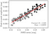 |
Fig. 7. Correlation between Polaris’ growing photometric amplitude and mean magnitude as measured by SMEI. The observations cover a total baseline of 8.65 yr, lasting until 17 days after the first spectroscopic observations were made with Hermes. Observing date is color coded in grayscale to illustrate the increasing amplitude and mean magnitude with time. The red solid line is a least squares fit to the data with the slope and Pearson’s correlation coefficient as indicated. |
Our reanalysis of the SMEI data leads to several surprising realizations. First, there is no straightforward astrophysical explanation for the correlation between amplitude and mean magnitude8. Previous studies of SMEI observations likely overlooked this correlation because of detrending algorithms applied to the data. Second, the SMEI photometric amplitude increased linearly over the full 8.65 yr timespan, which includes Hermes epoch (a). It seems rather unlikely that such a long-lasting amplitude increase of astrophysical origin should have all of a sudden stopped at the beginning of the Hermes observations, which rule out RV amplitude variations at the level of 1.7% (< 30 m s−1 for K = 1.763 km s−1, cf. Table 1) over more than 7 years immediately following the SMEI observations. Third, a preliminary inspection of SMEI data for δ Cep, η Aql, and ζ Gem reveals correlations of similar scale and sign, albeit with larger scatter due to insufficient removal of obvious instrumental effects and larger gaps in the time series.
Pending a more detailed investigation of SMEI’s systematic uncertainties, we therefore caution that the previously reported amplitude increases based on SMEI data may be of instrumental origin. For instance, a change of the detector’s non-linearity properties could lead to a simultaneous increase in amplitude and mean magnitude.
4.3. On additional periodicities
Earlier studies reported the presence of additional periodicities based on RV data, although no agreement among the reported periods was established. Specifically, periods identified included signals at 17d, 34d, 40d, 45d, and 119d (Dinshaw et al. 1989; Lee et al. 2008; Bruntt et al. 2008). B+08 further reported signals on timescales around 2 − 6 d based on SMEI photometry and constrained additional RV signals with periods 3 − 50 d to an upper limit 100 m s−1.
The main difficulty in using RV data for a periodogram analysis is the removal of the incompletely sampled large amplitude orbital motion, especially in the case of the Hermes data that span pericenter passage. Despite this difficulty of searching for additional RV signals, we found that including slow linear trends of up to a few tens of m s−1 significantly improved the template fit results for Hermes data, cf. Sect. 2. We interpret these trends as compensating for a combination of orbital acceleration and RV signals with periods longer than the typical observing run of approximately 10 d. As expected by this interpretation, we find the weakest trend of −3.9 m s−1 d−1 during epoch (g), which features by far the longest time span of 35 d (all other epochs cover < 11 d). Hence, the 40 d signal previously identified by Hatzes & Cochran (2000, henceforth: HC00) based on spectral line bisector variations in two different transitions (Sc II λ5527 Å and Mg I λ5528 Å) could potentially explain the per-epoch trends observed in Hermes RVs. We further note that the magnitude of the per-epoch trends (≤57.6 m s−1 d−1) is roughly consistent with the upper limit of 100 m s−1 determined by B+08.
To more closely investigate additional periodicities in spectral data, it is desirable to consider quantities that provide precise information on a star’s intrinsic variability without being sensitive to orbital motion. The bisector inverse span (BIS) provides a simple and precise quantification of spectral line profile asymmetry that varies on the timescale of Ppuls in all of the hundreds of Cepheids observed by the Geneva Cepheid Radial Velocity Survey (Anderson et al., in prep.). BIS is defined as the velocity difference between the top and bottom parts of a CCF, see (Anderson 2016, henceforth: A16) for a detailed discussion of BIS variability in the long-period Cepheid ℓ Carinae. BIS measurements benefit from a much increased signal-to-noise ratio of CCFs compared to bisector measurements of individual spectral lines, and we estimate their short-term precision to be approximately 6 − 10 m s−1 based on groups of consecutive observations (cf. Appendix A). Hence the Hermes BIS measurements are a factor of 2 − 3 more precise than the Hermes RV measurements. This precision gain results from the fact that each BIS measurement is a differential quantity determined on a single observation. As a result, BIS is virtually unaffected by changes in the wavelength scale due to changing ambient pressure, which is the dominant RV uncertainty for Hermes data. Moreover, BIS is unaffected by orbital motion, which does not contribute to line asymmetry. In the case of the extremely high S/N CCFs of Polaris, the main systematic effect on BIS is the stability of the instrumental line profile, which is much better than the long-term wavelength-scale stability. Hence, BIS measurements are extremely well-suited to investigate additional periodicities intrinsic to Polaris.
We employ Lomb-Scargle periodograms (Lomb 1976; Scargle 1982) computed using the astropy package (Price-Whelan et al. 2018, Version 3.1) to search for additional periodicities in BIS data. We first compute periodograms for frequencies corresponding to periods between one year and half a day. After an initial inspection, we focus our attention to frequencies shorter than 0.3 cycles d−1. Inspired by the second-order Fourier series model that best fits the RV data and the typically non-sinusoidal BIS variations in Cepheids (e.g. A16), we compute the periodograms using two-term Fourier series. We carry out a standard pre-whitening procedure, successively searching for dominant peaks in the periodogram and removing a combined model of all previously identified frequencies before computing new residual periodograms. The modeled frequencies are determined as the frequency at the highest peak. We adopt the following functional form for this multi-periodic BIS model: vbis(t) = v0,bis + ∑i,j[ai,j · cos(2π j(t − E)/Pi) + bi,j · sin (2π j(t − E)/Pi)], where vbis denotes BIS velocities, a and b the coefficients of each Fourier harmonic j, Pi the periods of each signal, t observation date, and E the reference epoch. Figure 8 illustrates our results, starting with the window function of the BIS measurements, the first periodogram and three residual periodograms.
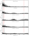 |
Fig. 8. Window function (top panel) and Lomb-Scargle periodograms of the successively pre-whitened Hermes BIS measurements. The three periods shown in Fig. 9 are indicated by vertical dashed red lines. The period subtracted in the previous step is marked by a solid black line in the following periodogram. Other notable peaks in the 2nd and 3rd panel from the top include the peak at twice Ppuls (2nd panel) and at twice P40d (third panel). |
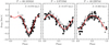 |
Fig. 9. BIS variations of Polaris measured from Hermes spectra phase-folded using three periods determined from Lomb-Scargle periodograms. Each panel shows the BIS variations associated with the periods indicated at the top (ΔvBIS). The signals at P60d = 60.16582 d, Ppuls = 3.97139 d, and P40d = 40.22074 d were identified using a successive pre-whitening procedure in this order. Second-order Fourier series models were fitted to the data using all three periods simultaneously and are shown separately for each signal as a solid red line. P60d and P40d are unlikely to be independent frequencies, since P40d/P60d = 0.6685 is suspiciously close to 2/3 while there remain phase gaps in the sampling of the 60 d signal. The signal at 40.2 d had previously been identified in bisector variations by HC00. We notice that the 40 d and 4 d signals have similar amplitude. The grayscale color coding traces observing date (white to black). |
The highest peak in the BIS periodogram occurs at 0.01662 c/d, i.e., at a period of 60.16582 d. After removing this signal, we find a dominant peak at the well-known pulsation period, Ppuls, together with its 0.5 c/d alias. After subtracting the combined model of the 60 d and Ppuls signals, we find two nearly equally high peaks at 0.02486 c/d and its 0.5 d alias (identified by phase folding the data with either signal). The successive removal of the three frequencies near 60.17 d, Ppuls, and 40.22 d reduces the RMS of the BIS measurements from 223 m s−1 to 135 m s−1 and 67 m s−1, respectively. The remaining RMS is relatively high compared to the precision estimate of the BIS measurements, leaving the possibility of there being additional signals beyond this three-period model. However, given the uncertain nature of the dominant 60 d signal, we conclude that additional observations are required to further investigate the multi-periodicity of Polaris. To test the significance of our results, we re-ran the analysis using sub-sets of the full data set, such as all even and all odd numbered observations, and confirmed the presence of the identified frequencies. We also repeated the analysis after splitting the data set in half (in time). The second half clearly reveals these signals, thanks to the dense sampling over a relatively short time, cf. Fig. 1, whereas the results based on the first half of the data set are less clear.
Figure 9 shows the BIS data phase-folded with each of these three periods after subtracting the model corresponding to the other two frequencies. As can be seen by the peak-to-peak amplitudes provided in each panel, the 60 d signal is the strongest of the three as expected from it having the highest peak in the BIS periodogram. However, it is suspicious that the ratio of the two periods 40.22074/60.16582 = 0.66850 ≈ 2/3, while the 60 d signal is not fully phase-sampled, cf. Fig. 9. Conversely, the signal at Ppuls and at 40.2 d are densely phase-sampled. The reality of the 40.2 d signal is strongly supported by HC00’s prior discovery based on an independent data set obtained in the years 1992–1993 with a different window function. We therefore consider the 40.22 d frequency a true signal of Polaris, whereas we caution that confirmation of the 60 d signal is needed. It is remarkable that the amplitude of the 40.22 d signal is essentially equal to the BIS signal at Ppuls even though its RVs counterpart is much weaker. Therefore, the 40.22 d signal primarily affects line shape, not line position, providing important constraints on the physical mechanism behind this signal, which may contribute to a clearer understanding of Polaris’ puzzling properties.
4.4. Is Polaris a fast rotator?
HC00 considered three different possible of origins of the 40 d bisector signal: macroturbulent spots, (magnetic) cool spots, and non-radial pulsations. Although they found no detailed model that could reproduce all the observed features, HC00 considered non-radial pulsations the most likely explanation, noting multiple additional periodicities reported in the literature as the most compelling reason for doing so. HC00 further explained that their model invoking surface inhomogeneities would imply high levels of magnetic activity, for which no evidence was available at the time. In particular, Polaris had not yet been detected in X-rays.
Meanwhile, X-rays from Polaris have been detected using Chandra (Evans et al. 2010), with LX = 28.89ergs−1 (0.3 − 8 keV), which was recently updated to LX = 28.8 − 29.2 erg s−1 (0.1 − 0.6 keV) (Engle et al. 2017). Additionally, detailed predictions of Cepheid properties based on Geneva stellar evolution models that incorporate the effects of rotation (Anderson et al. 2014, 2016a) can now be compared to Polaris’ observed properties, and in particular to investigate whether the 40.2 d BIS signal could originate in rotation.
To investigate the rotation hypothesis, we assume that the equatorial rotation period Prot = 40.2 d. The interferometrically measured diameter 3.123 mas (Mérand et al. 2006) projected to the distance implied by the Gaia DR2 parallax of Polaris B of 7.292 mas implies an equatorial rotation velocity vrot = 58.0 km s−1. Using vrotsini = 8.4 km s−1 from HC00 yields a very low inclination of i ∼ 8.3°. Thus, if the 40.2 d BIS signal were due to rotation, then Polaris would be seen nearly pole-on.
However, predictions based on Geneva models demonstrate that the rotation hypothesis is not consistent with observed properties of Polaris. The closest match to the implied surface rotation velocity is achieved by a 5 M⊙ first overtone Cepheid on the first instability strip crossing with Solar metallicity and very fast initial rotation (Ω/Ωcrit = 0.9) near the hot edge of the instability strip, with vrot = 55.6 km s−1 (Anderson et al. 2016a, their Table A.4). Observed CNO abundance ratios of [N/C] = 0.59 and [N/O] = 0.42 (Usenko et al. 2005) also agree with predictions for this model, cf. Figs. 10 and 11 in Anderson et al. (2014). However, neither the radius nor the absolute V-band magnitude of such a model are consistent with observations, with 26 R⊙ predicted vs. 46 R⊙ from interferometry and V = −2.6 mag predicted vs. −3.73 mag observed (Evans et al. 2018). To reach larger radii and greater luminosities would imply larger mass, which is disfavored by the recent astrometric mass measurement (Evans et al. 2018, 3.45 ± 0.75 M⊙). Moreover, higher mass would tend to reduce the surface rotation velocity during the Cepheid evolutionary phase.
We therefore conclude that a) rotation does not cause the 40.2 d BIS signal, and b) that the latest empirical mass and radius estimates, which assume the highly precise Gaia DR2 parallax of Polaris B, cannot be explained by ordinary single star evolution models. This is intriguing, since observed period-radius relations (Pilecki et al. 2018) and several other observables, incl. period-luminosity relations (Anderson et al. 2016a), agree closely with predictions based on the Geneva models. Alternative explanations of the intriguing 40.2 d BIS signal include non-radial pulsations as well as interactions between pulsations and the convective envelope (cf. A16 for modulated variability due to convection-pulsation interaction). Additional monitoring and analysis of Polaris’ BIS variability is required to further constrain the origin of this signal.
5. Conclusions
We present 161 high-precision RVs of the Cepheid Polaris Aa, measured on high-resolution optical spectra collected between 2011 and 2018. We investigate the stability of the Hermes RV curve over this duration using an empirical RV template fitting technique and demonstrate a stable RV amplitude to within ∼30 m s−1 over the 7 year timespan of the observations. The precise Hermes data provide evidence for additional RV signals that reveal themselves as slow linear trends over the typical 10 d duration of each observing epoch. The peak-to-peak amplitudes associated with these signals are on the order of ∼100 m s−1.
Applying the RV template fitting method to publicly accessible literature data, we find systematically different amplitudes between different data sets. However, no clear amplitude variations are recovered in any of the separately analyzed homogeneous data sets. We discuss the possibility of data inhomogeneity having contributed to reported RV amplitude differences in the literature. Additionally, we find strong indications that previously reported amplitude increases based on SMEI photometry were dominated by instrumental effects, which require detailed further investigation. Overall, we caution that Polaris’ amplitude may be and may have been much more stable than previously thought.
We determine an updated solution to the 29.32 yr orbit of Polaris based on pulsation-averaged velocities measured via the template fitting method applied to Hermes data and one large homogeneous literature data set (K96-08). The derived systemic velocity of the Polaris Aa-Ab system agrees with the Gaia DR2 measurement of the visual companion Polaris B to within the uncertainties.
We confirm line bisector variations with a period of 40.22 d that were originally discovered by HC00 using an independent set of bisector measurements of individual spectral lines. An additional periodicity of 60.17 d is indicated by the periodogram analysis, although we caution that this period may not be an independent frequency due to incomplete phase sampling and a suspicious period ratio of nearly 2/3 with the 40.22 d signal. We rule out a rotational origin of the 40.22 d BIS signal, which is most likely caused by non-radial pulsations or interactions between pulsations and the convective envelope.
Polaris is a truly enigmatic type-I Cepheid. By reconsidering and revising the puzzling accounts of its putative amplitude variations and additional periodicities, we have sought to facilitate a clearer understanding of this important star’s properties. Additional spectroscopic and photometric monitoring are now needed to fully unravel its multi-periodic signals, and new interferometric observations are required to better constrain its circumstellar environment. Both of these avenues should be pursued in order to explain Polaris’ properties and achieve a clearer understanding of the evolutionary paradigm of classical Cepheid variable stars.
Unless otherwise stated, Polaris shall refer to the Cepheid variable component Aa of the α UMi system using the nomenclature of Evans et al. (2008).
The 4 d periodicity due to pulsation was interpreted as orbital motion at the time.
Two different orbital models were used: the orbital solution obtained from a first pass with time-variable Ppuls, and the orbital solution derived from a combined Keplerian and Fourier Series fit to the Hermes data initialized at the K96 orbital period. Both approaches yield Ppuls consistent to within 0.25σ.
NB: Combining vγ values determined from literature data and Hermes is much more straightforward than comparing RV amplitudes related to pulsations, since orbital RV amplitudes do not depend on the spectral lines used in the measurement.
All amplitudes mentioned are peak-to-peak amplitudes.
A companion hypothesis involving the secular evolution of an unseen companion is easily ruled out based on the slope of the correlation.
Acknowledgments
This work would not have been possible without the help of several observers, including Lovro Palaversa, Berry Holl, Maria Süveges, Michał Pawlak, Andreas Postel, Kateryna Kravchenko, Maroussia Roelens, Nami Mowlavi, and May Gade Petersen. The competent and friendly assistance of the Mercator support staff and staff at KU Leuven’s astronomy department (in particular Jesus Perez Padilla, Saskia Prins, Florian Merges, Hans van Winckel, and Gert Rasking) is much appreciated. RIA thanks the anonymous referee for a timely and constructive report that helped to improve the manuscript. The author is furthermore pleased to extend a warm thanks to Dietrich Baade and Antoine Mérand for interesting discussions, as well as Byeong-Cheol Lee and Valery Kovtyukh for communications regarding Polaris. This research is based on observations made with the Mercator Telescope, operated on the island of La Palma by the Flemish Community, at the Spanish Observatorio del Roque de los Muchachos of the Instituto de Astrofísica de Canarias. Hermes is supported by the Fund for Scientific Research of Flanders (FWO), Belgium, the Research Council of K.U. Leuven, Belgium, the Fonds National de la Recherche Scientifique (F.R.S.-FNRS), Belgium, the Royal Observatory of Belgium, the Observatoire de Genève, Switzerland, and the Thüringer Landessternwarte, Tautenburg, Germany. This research has made use of NASA’s Astrophysics Data System; the SIMBAD database and the VizieR catalog access tool (http://cdsweb.u-strasbg.fr/) provided by CDS, Strasbourg; Astropy, a community-developed core Python package for Astronomy (Astropy Collaboration 2013; Price-Whelan et al. 2018);
References
- Anderson, R. I. 2013, PhD Thesis, Université de Genève [Google Scholar]
- Anderson, R. I. 2014, A&A, 566, L10 [NASA ADS] [CrossRef] [EDP Sciences] [Google Scholar]
- Anderson, R. I. 2016, MNRAS, 463, 1707 (A16) [NASA ADS] [CrossRef] [Google Scholar]
- Anderson, R. I. 2018a, A&A, 611, L7 [NASA ADS] [CrossRef] [EDP Sciences] [Google Scholar]
- Anderson, R. I. 2018b, in The RR Lyrae 2017 Conference. Revival of the Classical Pulsators: from Galactic Structure to Stellar Interior Diagnostics, eds. R. Smolec, K. Kinemuchi, & R. I. Anderson, 6, 193 [NASA ADS] [Google Scholar]
- Anderson, R. I., Ekström, S., Georgy, C., et al. 2014, A&A, 564, A100 [NASA ADS] [CrossRef] [EDP Sciences] [Google Scholar]
- Anderson, R. I., Sahlmann, J., Holl, B., et al. 2015, ApJ, 804, 144 [NASA ADS] [CrossRef] [Google Scholar]
- Anderson, R. I., Saio, H., Ekström, S., Georgy, C., & Meynet, G. 2016a, A&A, 591, A8 [NASA ADS] [CrossRef] [EDP Sciences] [Google Scholar]
- Anderson, R. I., Mérand, A., Kervella, P., et al. 2016b, MNRAS, 455, 4231 [NASA ADS] [CrossRef] [Google Scholar]
- Anderson, R. I., Casertano, S., Riess, A. G., et al. 2016c, ApJ, 226, 18 [Google Scholar]
- Arellano Ferro, A. 1983, ApJ, 274, 755 [NASA ADS] [CrossRef] [Google Scholar]
- Astropy Collaboration (Robitaille, T. P., et al.) 2013, A&A, 558, A33 [NASA ADS] [CrossRef] [EDP Sciences] [Google Scholar]
- Baranne, A., Queloz, D., Mayor, M., et al. 1996, A&AS, 119, 373 [NASA ADS] [CrossRef] [EDP Sciences] [Google Scholar]
- Berdnikov, L. N., & Stevens, I. R. 2010, in Variable Stars, the Galactic halo and Galaxy Formation, eds. C. Sterken, N. Samus, & L. Szabados [Google Scholar]
- Bond, H. E., Nelan, E. P., Remage Evans, N., Schaefer, G. H., & Harmer, D. 2018, ApJ, 853, 55 [NASA ADS] [CrossRef] [Google Scholar]
- Bruntt, H., Evans, N. R., Stello, D., et al. 2008, ApJ, 683, 433 (B+08) [NASA ADS] [CrossRef] [Google Scholar]
- Buffington, A., Band, D. L., Jackson, B. V., Hick, P. P., & Smith, A. C. 2006, ApJ, 637, 880 [NASA ADS] [CrossRef] [Google Scholar]
- Butler, R. P. 1993, ApJ, 415, 323 [NASA ADS] [CrossRef] [Google Scholar]
- Campbell, W. W. 1898, ApJ, 8 [Google Scholar]
- Campbell, W. W. 1899, ApJ, 10 [Google Scholar]
- Cropper, M., Katz, D., Sartoretti, P., et al. 2018, A&A, 616, A5 [NASA ADS] [CrossRef] [EDP Sciences] [Google Scholar]
- Derekas, A., Plachy, E., Molnár, L., et al. 2017, MNRAS, 464, 1553 [NASA ADS] [CrossRef] [Google Scholar]
- Dinshaw, N., Matthews, J. M., Walker, G. A. H., & Hill, G. M. 1989, AJ, 98, 2249 [NASA ADS] [CrossRef] [Google Scholar]
- Engle, S. G., Guinan, E. F., Harper, G. M., et al. 2017, ApJ, 838, 67 [NASA ADS] [CrossRef] [Google Scholar]
- Evans, N. R., Schaefer, G. H., Bond, H. E., et al. 2008, AJ, 136, 1137 [NASA ADS] [CrossRef] [Google Scholar]
- Evans, N. R., Guinan, E., Engle, S., et al. 2010, AJ, 139, 1968 [NASA ADS] [CrossRef] [Google Scholar]
- Evans, N. R., Szabó, R., Derekas, A., et al. 2015, MNRAS, 446, 4008 [NASA ADS] [CrossRef] [Google Scholar]
- Evans, N. R., Karovska, M., Bond, H. E., et al. 2018, ApJ, 863, 187 [NASA ADS] [CrossRef] [Google Scholar]
- Eyles, C. J., Simnett, G. M., Cooke, M. P., et al. 2003, Sol. Phys., 217, 319 [Google Scholar]
- Fernie, J. D., Kamper, K. W., & Seager, S. 1993, ApJ, 416, 820 [NASA ADS] [CrossRef] [Google Scholar]
- Gaia Collaboration (Brown, A. G. A., et al.) 2018, A&A, 616, A1 [NASA ADS] [CrossRef] [EDP Sciences] [Google Scholar]
- Gorynya, N. A., Irsmambetova, T. R., Rastorgouev, A. S., & Samus, N. N. 1992, Sov. Astron. Lett., 18, 316 [NASA ADS] [Google Scholar]
- Gorynya, N. A., Samus, N. N., Rastorguev, A. S., & Sachkov, M. E. 1996, Astron. Lett., 22, 175 [NASA ADS] [Google Scholar]
- Gorynya, N. A., Samus, N. N., Sachkov, M. E., et al. 1998, Astron. Lett., 24, 815 [NASA ADS] [Google Scholar]
- Grenfell, T. C., & Wallerstein, G. 1969, PASP, 81, 732 [NASA ADS] [CrossRef] [Google Scholar]
- Hatzes, A. P., & Cochran, W. D. 2000, AJ, 120, 979 (HC00) [NASA ADS] [CrossRef] [Google Scholar]
- Hertzsprung, E. 1911, Astron. Nachr., 189, 89 [NASA ADS] [CrossRef] [Google Scholar]
- Kamper, K. W. 1996, JRASC, 90, 140 (K96) [NASA ADS] [Google Scholar]
- Kamper, K. W., & Fernie, J. D. 1998, AJ, 116, 936 [NASA ADS] [CrossRef] [Google Scholar]
- Kamper, K. W., Evans, N. R., & Lyons, R. W. 1984, JRASC, 78, 173 [NASA ADS] [Google Scholar]
- Katz, D., Sartoretti, P., Cropper, M., et al. 2019, A&A, 622, A205 [NASA ADS] [CrossRef] [EDP Sciences] [Google Scholar]
- King, E. S. 1912, Popular Astron., 20, 505 [NASA ADS] [Google Scholar]
- Klagyivik, P., & Szabados, L. 2009, A&A, 504, 959 [NASA ADS] [CrossRef] [EDP Sciences] [Google Scholar]
- Kovacs, G., Kisvarsanyi, E. G., & Buchler, J. R. 1990, ApJ, 351, 606 [NASA ADS] [CrossRef] [Google Scholar]
- Lee, B.-C., Mkrtichian, D. E., Han, I., Park, M.-G., & Kim, K.-M. 2008, AJ, 135, 2240 [NASA ADS] [CrossRef] [Google Scholar]
- Lomb, N. R. 1976, Ap&SS, 39, 447 [NASA ADS] [CrossRef] [Google Scholar]
- Mérand, A., Kervella, P., Coudé du Foresto, V., et al. 2006, A&A, 453, 155 [NASA ADS] [CrossRef] [EDP Sciences] [Google Scholar]
- Moore, J. H. 1929, PASP, 41, 56 [NASA ADS] [CrossRef] [Google Scholar]
- Nardetto, N., Mourard, D., Mathias, P., Fokin, A., & Gillet, D. 2007, A&A, 471, 661 [NASA ADS] [CrossRef] [EDP Sciences] [Google Scholar]
- Pannekoek, A. 1913, Astron. Nachr., 194, 359 [NASA ADS] [CrossRef] [Google Scholar]
- Pepe, F., Mayor, M., Galland, F., et al. 2002, A&A, 388, 632 [NASA ADS] [CrossRef] [EDP Sciences] [Google Scholar]
- Petterson, O. K. L., Cottrell, P. L., Albrow, M. D., & Fokin, A. 2005, MNRAS, 362, 1167 [NASA ADS] [CrossRef] [Google Scholar]
- Pilecki, B., Gieren, W., Pietrzyński, G., et al. 2018, ApJ, 862, 43 [NASA ADS] [CrossRef] [Google Scholar]
- Poleski, R. 2008, Acta Astron., 58, 313 [NASA ADS] [Google Scholar]
- Poretti, E., Le Borgne, J. F., Rainer, M., et al. 2015, MNRAS, 454, 849 [NASA ADS] [CrossRef] [Google Scholar]
- Price-Whelan, A. M., Sipőcz, B. M., Günther, H. M., et al. 2018, AJ, 156, 123 [Google Scholar]
- Raskin, G., van Winckel, H., Hensberge, H., et al. 2011, A&A, 526, A69 [NASA ADS] [CrossRef] [EDP Sciences] [Google Scholar]
- Riess, A. G., Macri, L. M., Hoffmann, S. L., et al. 2016, ApJ, 826, 56 [NASA ADS] [CrossRef] [Google Scholar]
- Riess, A. G., Casertano, S., Yuan, W., et al. 2018, ApJ, 861, 126 [Google Scholar]
- Roemer, E. 1965, ApJ, 141, 1415 [NASA ADS] [CrossRef] [Google Scholar]
- Scargle, J. D. 1982, ApJ, 263, 835 [NASA ADS] [CrossRef] [Google Scholar]
- Seidel, P. L. 1852, Mathematisch-Physikalische Klasse (Bayerische Staatsbibliothek), 6, 539 [Google Scholar]
- Smolec, R. 2017, MNRAS, 468, 4299 [NASA ADS] [CrossRef] [Google Scholar]
- Spreckley, S. A., & Stevens, I. R. 2008, MNRAS, 388, 1239 [NASA ADS] [Google Scholar]
- Süveges, M., & Anderson, R. I. 2018, A&A, 610, A86 [NASA ADS] [CrossRef] [EDP Sciences] [Google Scholar]
- Tokovinin, A. A. 1987, Sov. Astron., 31, 98 [NASA ADS] [Google Scholar]
- Turner, D. G., Savoy, J., Derrah, J., Abdel-Sabour Abdel-Latif, M., & Berdnikov, L. N. 2005, PASP, 117, 207 [NASA ADS] [CrossRef] [Google Scholar]
- Udry, S., Mayor, M., Maurice, E., et al. 1999, in IAU Colloq. 170: Precise Stellar Radial Velocities, eds. J. B. Hearnshaw, C. D. Scarfe, ASP Conf. Ser., 185, 383 [NASA ADS] [Google Scholar]
- Usenko, I. A., Miroshnichenko, A. S., Klochkova, V. G., & Yushkin, M. V. 2005, MNRAS, 362, 1219 [NASA ADS] [CrossRef] [Google Scholar]
- Usenko, I. A., Kovtyukh, V. V., Miroshnichenko, A. S., Danford, S., & Prendergast, P. 2018, MNRAS, 481, L115 [NASA ADS] [CrossRef] [Google Scholar]
- Švanda, M., & Harmanec, P. 2017, Res. Notes AAS, 1, 39 [CrossRef] [Google Scholar]
Appendix A: Hermes RVs of Polaris Aa
Table A.1 lists the Hermes measurements presented here. The full list of measurements is available via the CDS.
Subset of Hermes RV and BIS measurements used in this work.
Appendix B: Figures showing RV template fitting method applied to literature RVs
Figure B.1 shows the RV template fits applied to K96-08 data; the residuals as a function of time are shown in Fig. B.2. Figure B.3 shows the template fits to the K96-CE data.
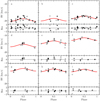 |
Fig. B.1. RV template fitting method applied to high-dispersion photographic RVs by Kamper (1996) (K96-08). No significant amplitude variation is seen with time, although the orbital motion is clearly apparent. |
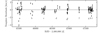 |
Fig. B.2. Residuals from RV template fitting method applied to K96-08 RVs. The improvement of the RV precision following “standardization” of the RV measurement following Arellano Ferro (1983) is clearly seen. |
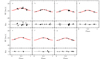 |
Fig. B.3. RV template fitting method applied to K96-CE RVs. No significant variation in amplitude is apparent with time, although the scatter in the first three epochs is significantly larger than in the later four, likely because of calibration issues. |
Appendix C: SMEI per-epoch Fourier series fits
Figure C.1 shows the Fourier series fits to the 100 sub-epochs of SMEI observations used in Sect. 4.2.
 |
Fig. C.1. Second-order Fourier series models fitted to 100 sub-epochs of SMEI data, cf. Sect. 4.2. Insufficient data were available for the 27th epoch. Peak-to-peak amplitudes are indicated in each panel. Time increases across the figure from left to right and top to bottom. In each panel, observation dates are grayscaled from white to black. The ordinate (SMEI magnitude) and abscissa (phase) ranges are −0.05 to 0.05 mag and −0.1 to 1.1, respectively, in all panels. |
All Tables
Results from the template fitting analysis applied to RV data of Polaris from Hermes, Kamper (1996), and Gorynya et al. (1992).
All Figures
|
Fig. 1. Hermes radial velocity curve of Polaris as a function of observing date. The short term scatter is due to the ∼4 d pulsation, the long-term variations reveal the orbital motion whose pericenter passage occurred in late 2016. |
| In the text | |
|
Fig. 2. RVs of Polaris at the reference epoch (c) chosen for its densest phase coverage over a short timescale. Top panel: Hermes data as a function of Barycentric Julian Date with the overplotted model consisting of the reference Fourier series model and a slow linear term of 9 ± 1 m s−1 d−1. Bottom panel: residuals of the fit, with an RMS of 13 m s−1. The grayscale traces observing date as is done for the template fits below. |
| In the text | |
|
Fig. 3. Per-epoch template fits to Hermes RV data. In each panel, a gray scale is applied to distinguish the observing data internal to the given epoch, i.e., the gray scale runs from white to black among the measurements of that epoch. For each epoch, we show the Hermes data phase-folded and zero-phase shifted as determined from the template fit. The red solid curve in each panel is the pulsation model (cf. Fig. 2), shifted to the vγ of that epoch. Fit residuals are shown underneath each template fit, and a grayscale traces observing date in each epoch (white to black). |
| In the text | |
|
Fig. 4. Hermes RV template fit residuals as a function of observing date. The highest scatter is found in epoch (e), which is near pericenter passage and thus the most sensitive to orbital motion. |
| In the text | |
|
Fig. 5. Radial velocity data from Kamper (1996) measured at DDO. Different symbols and colors are used to distinguish data measured using different instrumental setups. Labels “08”, “12”, and “16” refer to photographic of different dispersions (in mm Å−1). “RE” refers to measurements taken using a Reticon detector, “CF” to ones using a fiber link, and “CE” to observations made using a CCD. Instrumental zero-point variations related to these interventions and associated calibration issues are readily apparent, especially following the peak of the orbital RV variation near HJD 2 445 750. |
| In the text | |
|
Fig. 6. Orbital solution based on the RV template fitting procedure applied to data from Hermes and the high-dispersion photographic RVs from Kamper (1996, K96-08 RVs). The K96-08 RVs have been zero-point corrected by 0.63 km s−1, cf. Sect. 3.3. |
| In the text | |
|
Fig. 7. Correlation between Polaris’ growing photometric amplitude and mean magnitude as measured by SMEI. The observations cover a total baseline of 8.65 yr, lasting until 17 days after the first spectroscopic observations were made with Hermes. Observing date is color coded in grayscale to illustrate the increasing amplitude and mean magnitude with time. The red solid line is a least squares fit to the data with the slope and Pearson’s correlation coefficient as indicated. |
| In the text | |
|
Fig. 8. Window function (top panel) and Lomb-Scargle periodograms of the successively pre-whitened Hermes BIS measurements. The three periods shown in Fig. 9 are indicated by vertical dashed red lines. The period subtracted in the previous step is marked by a solid black line in the following periodogram. Other notable peaks in the 2nd and 3rd panel from the top include the peak at twice Ppuls (2nd panel) and at twice P40d (third panel). |
| In the text | |
|
Fig. 9. BIS variations of Polaris measured from Hermes spectra phase-folded using three periods determined from Lomb-Scargle periodograms. Each panel shows the BIS variations associated with the periods indicated at the top (ΔvBIS). The signals at P60d = 60.16582 d, Ppuls = 3.97139 d, and P40d = 40.22074 d were identified using a successive pre-whitening procedure in this order. Second-order Fourier series models were fitted to the data using all three periods simultaneously and are shown separately for each signal as a solid red line. P60d and P40d are unlikely to be independent frequencies, since P40d/P60d = 0.6685 is suspiciously close to 2/3 while there remain phase gaps in the sampling of the 60 d signal. The signal at 40.2 d had previously been identified in bisector variations by HC00. We notice that the 40 d and 4 d signals have similar amplitude. The grayscale color coding traces observing date (white to black). |
| In the text | |
|
Fig. B.1. RV template fitting method applied to high-dispersion photographic RVs by Kamper (1996) (K96-08). No significant amplitude variation is seen with time, although the orbital motion is clearly apparent. |
| In the text | |
|
Fig. B.2. Residuals from RV template fitting method applied to K96-08 RVs. The improvement of the RV precision following “standardization” of the RV measurement following Arellano Ferro (1983) is clearly seen. |
| In the text | |
|
Fig. B.3. RV template fitting method applied to K96-CE RVs. No significant variation in amplitude is apparent with time, although the scatter in the first three epochs is significantly larger than in the later four, likely because of calibration issues. |
| In the text | |
|
Fig. C.1. Second-order Fourier series models fitted to 100 sub-epochs of SMEI data, cf. Sect. 4.2. Insufficient data were available for the 27th epoch. Peak-to-peak amplitudes are indicated in each panel. Time increases across the figure from left to right and top to bottom. In each panel, observation dates are grayscaled from white to black. The ordinate (SMEI magnitude) and abscissa (phase) ranges are −0.05 to 0.05 mag and −0.1 to 1.1, respectively, in all panels. |
| In the text | |
Current usage metrics show cumulative count of Article Views (full-text article views including HTML views, PDF and ePub downloads, according to the available data) and Abstracts Views on Vision4Press platform.
Data correspond to usage on the plateform after 2015. The current usage metrics is available 48-96 hours after online publication and is updated daily on week days.
Initial download of the metrics may take a while.