| Issue |
A&A
Volume 623, March 2019
|
|
|---|---|---|
| Article Number | A8 | |
| Number of page(s) | 32 | |
| Section | Stellar structure and evolution | |
| DOI | https://doi.org/10.1051/0004-6361/201834360 | |
| Published online | 25 February 2019 | |
Low-metallicity massive single stars with rotation
II. Predicting spectra and spectral classes of chemically homogeneously evolving stars
1
Astronomický ústav, Akademie věd České republiky, Fričova 298, 251 65 Ondřejov, Czech Republic
e-mail: brankica.kubatova@asu.cas.cz
2
School of Physics and Astronomy and Institute of Gravitational Wave Astronomy, University of Birmingham, Edgbaston, Birmingham B15 2TT, UK
3
Institut für Physik und Astronomie, Universität Potsdam, Karl-Liebknecht-Str. 24/25, 14476 Potsdam, Germany
4
Armagh Observatory and Planetarium, College Hill, Armagh BT61 9DG, UK
5
European Space Astronomy Centre (ESA/ESAC), Operations Department, 28692 Villanueva de la Cañada, Madrid, Spain
6
Ústav teoretické fyziky a astrofyziky, Masarykova univerzita, Kotlářská 267/2, 611 37 Brno, Czech Republic
7
Instituto de Astrofísica de Andalucía (IAA/CSIC), Glorieta de la Astronomía s/n Aptdo. 3004, 18080 Granada, Spain
8
Institute of Astrophysics, KU Leuven, Celestijnenlaan 200 D, 3001 Leuven, Belgium
9
Institute for Astronomy, Astrophysics, Space Applications & Remote Sensing, National Observatory of Athens, Vas. Pavlou and I. Metaxa, Penteli 15236, Greece
Received:
2
October
2018
Accepted:
9
January
2019
Context. Metal-poor massive stars are assumed to be progenitors of certain supernovae, gamma-ray bursts, and compact object mergers that might contribute to the early epochs of the Universe with their strong ionizing radiation. However, this assumption remains mainly theoretical because individual spectroscopic observations of such objects have rarely been carried out below the metallicity of the Small Magellanic Cloud.
Aims. Here we explore the predictions of the state-of-the-art theories of stellar evolution combined with those of stellar atmospheres about a certain type of metal-poor (0.02 Z⊙) hot massive stars, the chemically homogeneously evolving stars that we call Transparent Wind Ultraviolet INtense (TWUIN) stars.
Methods. We computed synthetic spectra corresponding to a broad range in masses (20−130 M⊙) and covering several evolutionary phases from the zero-age main-sequence up to the core helium-burning stage. We investigated the influence of mass loss and wind clumping on spectral appearance and classified the spectra according to the Morgan-Keenan (MK) system.
Results. We find that TWUIN stars show almost no emission lines during most of their core hydrogen-burning lifetimes. Most metal lines are completely absent, including nitrogen. During their core helium-burning stage, lines switch to emission, and even some metal lines (oxygen and carbon, but still almost no nitrogen) are detected. Mass loss and clumping play a significant role in line formation in later evolutionary phases, particularly during core helium-burning. Most of our spectra are classified as an early-O type giant or supergiant, and we find Wolf–Rayet stars of type WO in the core helium-burning phase.
Conclusions. An extremely hot, early-O type star observed in a low-metallicity galaxy could be the result of chemically homogeneous evolution and might therefore be the progenitor of a long-duration gamma-ray burst or a type Ic supernova. TWUIN stars may play an important role in reionizing the Universe because they are hot without showing prominent emission lines during most of their lifetime.
Key words: stars: massive / stars: winds, outflows / stars: rotation / galaxies: dwarf / radiative transfer
© ESO 2019
1. Introduction
Low-metallicity massive stars are essential building blocks of the Universe. Not only do these objects play a role in cosmology by contributing to the chemical evolution of the early Universe and the reionization history (e.g., Abel et al. 2002; Yoshida et al. 2007; Sobral et al. 2015; Matthee et al. 2018), they may also influence the structure of low-metallicity dwarf galaxies in the local Universe (e.g., Tolstoy et al. 2009; Annibali et al. 2013; Weisz et al. 2014). Moreover, they may lead to spectacular explosive phenomena such as supernovae (e.g., Quimby et al. 2011; Inserra et al. 2013; Lunnan et al. 2013), gamma-ray bursts (e.g., Levesque et al. 2010; Modjaz et al. 2011; Vergani et al. 2015), and possibly even gravitational wave-emitting mergers (e.g., Abbott et al. 2016, 2017). The details of all these processes, however, are still veiled by many uncertainties because low-metallicity (< 0.2 Z⊙) massive stars have rarely been analyzed by quantitative spectroscopy as individual objects: the instrumentation necessary to obtain the required data quality has only recently become available. Individual spectral analyses of massive stars have been published only down to 0.1 Z⊙, such as one Wolf–Rayet (WR) star of type WO in the galaxy IC 1613 (Tramper et al. 2013) and several hot stars in the galaxies IC 1613, WLM, and NGC 3109 (e.g., Tramper et al. 2011, 2014; Herrero et al. 2012; Garcia et al. 2014; Bouret et al. 2015; Camacho et al. 2016). Additionally, massive stars have been studied in the Small Magellanic Cloud (SMC) at ZSMC ∼ 0.2 Z⊙, including 10 red supergiants (Davies et al. 2015), 12 WR stars (Hainich et al. 2015; Massey et al. 2015; Shenar et al. 2016), and a few hundred O-type stars (Lamb et al. 2016).
At metallicities below 0.1 Z⊙, however, no direct spectroscopic observations of individual massive stars have been reported so far. Although such stars might have been contributing to our Galaxy’s chemical composition in the past (specifically in globular clusters, see, e.g., Szécsi et al. 2018; Szécsi & Wünsch 2019), they no longer exist in our Galaxy. Even if the second generation of stars in the early Universe was indeed composed of many massive and very massive stars (e.g., Choudhury & Ferrara 2007; Ma et al. 2017), our observing capacities are not sufficient to look that far for individual objects.
Even in local star-forming dwarf galaxies it is hard to resolve massive stars individually because they are embedded in dense and gaseous OB associations (Shirazi & Brinchmann 2012; Kehrig et al. 2013). However, we may be able to find indirect traces of their existence, such as the total amount of ionizing photons emitted by them, or the integrated emission lines of their WR stars (Kehrig et al. 2015; Szécsi et al. 2015a,b). Future observing campaigns may even provide us with a census of massive stars in metal-poor dwarf galaxies such as Sextant A (∼1/7 Z⊙, McConnachie 2012) or I Zwicky 18 (∼1/40 Z⊙, Kehrig et al. 2016).
In this paper, we focus on a certain exotic type of low-metallicity massive stars: those that are fast rotating and evolve chemically homogeneously. Szécsi et al. (2015b, hereafter Paper I) called their core hydrogen-burning (CHB) phases TWUIN stars; the term stands for Transparent Wind Ultraviolet INtense. These stars were so named because they were predicted to have weak, optically thin stellar winds while being hot, and thus emitting most of their radiation in the UV band (for more details, see Szécsi et al. 2015a,b; Szécsi 2016, 2017a,b). TWUIN stars have extensively been investigated from an evolutionary point of view, mainly as a means to explain cosmic explosions and mergers. They were referred to as “stars with chemically homogeneous evolution” and “fast-rotating He-stars” by Yoon & Langer (2005) and Yoon et al. (2006), who showed that they may be applied as single-star progenitors of long-duration gamma-ray bursts and supernovae of type Ib/c. They were referred to as “stars that evolve chemically homogeneously” by Brott et al. (2011), who presented such single-star models with SMC metallicity. They were referred to as “the quasi-chemically homogeneous massive stars” by Cantiello et al. (2007), who created such models to account for long-duration gamma-ray bursts, this time through binary interaction at ZSMC. They were referred to as “Wolf–Rayet stars in disguise” by de Mink et al. (2009), who showed that such binaries may finally form a double black-hole system. The latter hypothesis was further elaborated on by de Mink & Mandel (2016) and Mandel & de Mink (2016), as well as by Marchant et al. (2016, 2017), to provide progenitor channels to gravitational-wave emission. In particular, Marchant et al. (2016) found that chemically homogeneous stars at ∼0.02 Z⊙ (indeed what we call TWUIN stars here), when in a close binary, predict the highest rate of double black-hole mergers compared to other metallicities.
All these authors were mainly concerned with either the inner structure or the final fate of these stars, but rarely with their appearance. Theorists sometimes called them simply WR stars (e.g., Cui et al. 2018) because their surface composition and temperature, as predicted by the evolutionary models, are similar to those of observed WR stars. However, to determine whether they are in fact WR stars from an observational point of view (i.e., if they show broad and bright emission lines in the optical region), their spectral appearance needs to be known. A pioneer study in this direction was recently carried out by Hainich et al. (2018).
This is the second paper of a series. In Paper I we presented stellar evolutionary computations of TWUIN stars (see Sects. 6 and also 10.4) during the CHB phase, while some of these models were followed over the core helium-burning (CHeB) phase in Szécsi (2016, see Chapter 4 of the thesis). In the current paper, we now simulate the atmospheres and spectra of chemically homogeneously evolving stars of different masses and cover their whole evolution. We use the the Potsdam Wolf-Rayet (PoWR) stellar atmosphere code to compute the synthetic spectra. The initial metallicity of the evolutionary models based on which the synthetic spectra are created is 0.02 Z⊙. The choice of this particular metallicity value is motivated by the fact that binary models of this metallicity have been successfully applied in the context of double compact object progenitors (e.g., Marchant et al. 2016) as well as other explosive phenomena (see the review of Szécsi 2017b), and that such stars might be found in some local dwarf galaxies (Szécsi et al. 2015a). We explore the expected observable characteristics of these stars, classify them accordingly, and provide the spectral features that can be used to guide targeted observing campaigns. The predicted spectra are later applied to create a synthetic population to be compared to observational properties of low-metallicity dwarf galaxies in a next part of this series.
This paper is organized as follows: In Sect. 2 we give an overview of the stellar evolutionary model sequences used in this work. In Sect. 3 we present the stellar atmosphere and wind models. In particular, stellar parameters and chemical composition are summarized in Sect. 3.1, while the wind properties are described in Sect. 3.1. In Sect. 4 we provide synthetic spectra of chemically homogeneously evolving stars. The effects of mass loss and wind clumping on line formation are presented in Sects. 4.2 and 4.3, respectively. Classifications of the model spectra are presented in Sect. 5. In Sect. 6 we discus the validity of the models and suggest future research directions. Finally, a summary is given in Sect. 7. All the calculated spectra are available in Appendix B.
2. Stellar evolutionary model sequences
Single stellar evolutionary sequences of low-metallicity (Z ∼ 0.02 Z⊙ or [Fe/H] = −1.7), fast-rotating massive stars were computed in Paper I for the CHB phase. The sequences were created using the Bonn evolutionary code (BEC). For the details of the code and the initial parameters of the computations, we refer to Paper I and references therein. Because we are also interested in further hydrogen-free evolution, we rely on the work of Szécsi (2016), who continued the computation of these sequences during CHeB until helium exhaustion in the core. To represent different evolutionary stages with spectra, we use three chemically homogeneously evolving sequences: those with initial masses Mini of 20 M⊙, 59 M⊙, and 131 M⊙, and initial rotational velocities of 450 km s−1, 300 km s−1, and 600 km s−1, respectively. These three tracks are shown in Fig. 1.
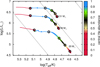 |
Fig. 1. HR diagram of our models (black symbols) and their corresponding evolutionary sequences. The sequences are taken from Paper I and Szécsi (2016). Initial masses are labeled, showing where the tracks start their evolution, proceeding toward the hot side of the diagram. Colors show the central helium mass fraction, and dots represent every 105 years of evolution. Dashed lines mark equiradial lines with 1, 10, and 100 R⊙ from left to right. The black symbols represent the models for which we computed synthetic spectra. From right to left: black symbols correspond to evolutionary phases with surface helium mass fractions of 0.28, 0.5, 0.75, and 0.98, and the fifth symbol on the very left corresponds to a central helium mass fraction of 0.5, i.e., the middle of the CHeB phase. |
All three evolutionary sequences are computed assuming initial fast rotation, which is inherited from the 15 models that we compute spectra for. Their rotational velocities are in the range of 400 − 1000 km s−1 (see Table 1), which is still not close the critical rotational limit of these massive stars (∼0.4−0.6 vcrit). Therefore, we do not expect these stars to form a decretion disk. Additionally, although these velocities may seem extremely high, a very similar evolution is found at lower rotational rates as well. For example, the model with Mini = 131 M⊙ rotates with about 800 − 900 km s−1 in the first part of its CHB lifetime, and the model rotating only with 450 km s−1 in this phase evolves in almost exactly the same way (cf. Fig. 4 in Paper I). As discussed in Sect. 10.4 of Paper I, it is expected that about 20% of all massive stars at this metallicity evolve chemically homogeneously because of their fast rotation; indeed, observations down to ZSMC suggest that stellar rotation increases with lower metallicity (Mokiem et al. 2006; Martayan et al. 2007).
Main parameters of the 15 model stars.
To simulate the wind structure and spectra, we chose four models for each track: those with a surface helium mass fraction, YS, of 0.28, 0.5, 0.75, and 0.98, as well as one model per track for the CHeB phase, as shown in Fig. 1 (note the color coding in the figure showing the central helium mass fraction, YC, of the model sequences, which reflects the evolutionary stage) and in Table 1.
2.1. Mass loss applied to the evolutionary sequences
Mass loss of massive stars may influence their evolution significantly even at this low metallicity (see Paper I). The sequences were computed assuming a prescription for radiation-driven mass loss of hot O-type stars (Vink et al. 2000, 2001) providing the mass-loss rate Ṁ as a function of initial metal abundance Zini (given in units of solar metallicity Z⊙) and further stellar parameters:
![$$ \begin{aligned}&\log \frac{{\dot{M}}}{M_{\odot }/\mathrm{{yr}}} = -6.7 + 2.2 \log \left({L_*/10^5}\right) - 1.3 \log \left({M_*/30}\right) \nonumber \\&\qquad \qquad \quad \quad - 1.2 \log \left({\frac{v_{\infty }/{v_{\rm {esc}}}}{2.0}}\right) + 0.9 \log \left({{T_{\rm {eff}}}/40\,000}\right)\nonumber \\&\qquad \qquad \quad \quad - 10.9 \left[{\log \left({{T_{\rm {eff}}}/40\,000}\right)}\right]^2 + 0.85 \log ({Z_{\mathrm{ini} }}/{Z_{\odot }}), \end{aligned} $$](/articles/aa/full_html/2019/03/aa34360-18/aa34360-18-eq1.gif)
where Ṁ is in units of M⊙/yr, stellar effective temperature Teff is in units of Kelvin, stellar mass M* and luminosity L* are in solar units; the ratio of the terminal velocity v∞ and escape velocity vesc are taken as v∞/vesc = 2.6 for the evolutionary models because they all are above the bistability jump (Lamers et al. 1995; Vink et al. 2000). This formula was applied when YS was lower than 0.55, which is true for every first two models of our three evolutionary sequences (i.e., the T-1, T-2, T-6, T-7, T-11, and T-12 models, cf. Table 1). Because the models evolve chemically homogeneously, the surface abundances are very close to those in the core, YS ∼ YC.
A different prescription was assumed for phases when YS > 0.7, which applies for WR stars,
used for models T-3, T-4, T-8, T-9, T-13, and T-14. Here XS is the surface hydrogen mass fraction. This expression follows from Eq. (2) in Hamann et al. (1995), but has been reduced by a factor of 10, as suggested by Yoon et al. (2006). The reduction by 10 gives a mass-loss rate comparable to the commonly adopted rate reported by Nugis & Lamers (2000; see Fig. 1 in Yoon 2015). For the dependence on XS, see the steepness of the fit in Fig. 7 of Hamann et al. (1995).
During the whole CHeB phase, the WR-type prescription of Eq. (2) was applied everywhere (models T-5, T-10, and T-15).
2.2. Uncertainties in the mass-loss prediction
Many uncertainties are associated with this treatment of the wind mass loss. For example, the prescription in Eq. (2) includes a metallicity dependence of  following Vink et al. (2001). In reality, however, the dependence may be weaker than this (i.e., real winds are stronger than assumed), as suggested by theoretical calculations for classic WR stars in Vink & de Koter (2005) and Eldridge & Vink (2006). Conversely, observations of WN stars carried out by Hainich et al. (2015) found a stronger dependence (i.e., real winds are weaker than assumed). It seems therefore that the question of the metallicity dependence of WR winds remains to be settled.
Additionally, WN stars and WC stars may well be different from each other when it comes to wind mass loss; and both are quite different from the CHB phase of our chemically homogeneously evolving models (when they are TWUIN stars). Still, the reason in Paper I for using a mass-loss rate prescription based on observations of WR stars to simulate TWUIN stellar evolution was that in terms of surface composition and temperature, WR stars are the objects that are most similar to TWUIN stars. We provide suggestions for future research directions to establish the wind properties of TWUIN stars (both observationally and theoretically) in Sects. 6.3 and 6.4.
To account for all these uncertainties, we created two versions for every model. One has a nominal mass-loss rate as implemented in the evolutionary models, that is, according to Eqs. (1) and (2). The other has a reduced value that is a factor 100 lower than the nominal value. Choosing a factor of 100 is motivated by the work of Hainich et al. (2015), who found a steeper metallicity-dependence of WR winds. This is to say that using the mass-loss prescription given by Eq. (11) of Hainich et al. (2015), we obtained mass-loss rates that were similar to our reduced values; see Table 2. We refer to the nominal value as “higher”, which means in the context of our study that it is the higher value of the two. By testing these two rather extreme values, we account for uncertainties in the mass-loss predictions of these stars.
Mass-loss rate values applied in the synthetic spectra computations, compared to those that Hainich et al. (2015) would predict for the same stars.
3. Stellar atmosphere and wind models
To calculate the synthetic spectra and to obtain the stratification of wind parameters, a proper modeling of the static and expanding atmosphere is required. We calculated stellar spectra by means of the Potsdam Wolf-Rayet (PoWR) atmosphere code. Because the PoWR code treats both quasi-static (i.e., photospheric) and expanding layers (i.e., wind) of the stellar atmosphere consistently, it is applicable to most types of hot stars.
The PoWR code solves the non-local thermal equilibirum (non-LTE) radiative transfer in a spherically expanding atmosphere with a stationary mass outflow. A consistent solution for the radiation field and the population numbers is obtained iteratively by solving the equations of statistical equilibrium and radiative transfer in the comoving frame (Mihalas 1978; Hubeny & Mihalas 2014). After an atmosphere model is converged, the synthetic spectrum is calculated by a formal integration along emerging rays.
To ensure energy conservation in the expanding atmosphere, the temperature stratification is updated iteratively using the electron thermal balance method (Kubát et al. 1999) and a generalized form of the so-called Unsöld-Lucy method, which assumes radiative equilibrium (Hamann & Gräfener 2003). In the comoving frame calculations during the non-LTE iteration, the line profiles are assumed to be Gaussians with a constant Doppler broadening velocity vD, which accounts for broadening due to thermal and microturbulent velocities. In this work we use vD = 100 km s−1. All spectra correspond to being seen edge-on, that is, the lines are fully broadened by rotation.
After the model iteration converged and all population numbers are established, the emergent spectrum is finally calculated in the observer’s frame, using a refined set of atomic data (e.g., with multiplet splitting) and accounting in detail for thermal, microturbulent, and pressure broadening of the lines. Detailed information on the assumptions and numerical methods used in the code can be found in Gräfener et al. (2002), Hamann & Gräfener (2003, 2004), and Sander et al. (2015).
3.1. Stellar parameters and chemical composition
Fundamental stellar parameters required as input for PoWR model atmosphere calculations are the stellar temperature T*, the stellar mass M*, and the stellar luminosity L*. These were adopted from the stellar evolutionary model sequences (see Table 1), assuming that the hydrostatic surface temperature Teff of the BEC evolutionary models coincides with T*. With given L* and T*, the stellar radius R* was calculated via Stefan-Boltzmann’s law
where σSB is the Stefan-Boltzmann constant. In the PoWR code the temperature T* is an effective temperature at the radius R*, which is defined at the Rosseland continuum optical depth τmax = 20. The outer atmosphere (i.e., wind) boundary is set to 1000 R* with the exception of the models for Mini = 20 M⊙, where 100 R* is already sufficient. Further details about the method of model atmosphere calculations can be found in Sander et al. (2015).
Detailed model atoms of all relevant elements are taken into account. Line blanketing is considered with the iron-group elements treated in the super-level approach, accounting not only for Fe, but also for Sc, Ti, V, Cr, Mn, Co, and Ni (see Gräfener et al. 2002, for details). The abundances of H, He, C, N, O, Ne, Mg, Al, Si, and Fe are adopted from the stellar evolutionary model sequences. The additional elements such as P, S, Cl, Ar, K, and Cl, which are not considered in the stellar evolutionary models but are used in the PoWR model atmosphere calculations, are also considered in a minimum-level approach to account for their potential contributions to the wind driving. The additional elements have abundances of Z⊙/50. For iron group elements we consider the ionization stages from I up to XVII to ensure that all sources that significantly contribute to opacity are taken into account. Higher ionization stages of Fe are important especially for the CHeB stages of the considered stars.
3.2. Wind properties
Because we consider objects that were predicted only theoretically and have never been observed, there exist no observational constraints on their wind properties so far. Within the frame of model consistency, there is therefore some freedom in adopting atmospheric and wind parameters.
Mass-loss rates. With specified Ṁ in the PoWR code, the density stratification ρ(r) in the wind is calculated via the continuity equation given as
To be consistent with stellar evolutionary models that provide the basis for our spectral models, we decided to apply the same mass-loss rate values as in these models. We note that these values were assumed in the evolutionary models based on prescribed recipes (see Sect. 2.1) and are not predicted by the models. To test the effect of mass loss on the emergent spectra, we therefore supplemented our work by another set of models: one model calculated with a mass-loss rate that is hundred times lower than in the original set (see Table 2 and Sect. 2.1). This enables us to roughly estimate uncertainties of our emergent radiation prediction due to uncertainties in the choice of mass-loss rates.
Velocity. The adopted velocity field in the PoWR models consists of two parts. A hydrostatic part where gravity is balanced by gas and radiation pressure, and a wind part where the outward pressure exceeds gravity and therefore the matter is accelerated. To properly account for the velocity field in the inner part of the wind, the quasi-hydrostatic part of the atmosphere is calculated self-consistently to fulfill the hydrostatic equation. Computing hydrodynamically consistent stellar atmosphere models this way is a new approach, recently implemented in the PoWR code (see Sander et al. 2015). In the wind domain (i.e., the supersonic part), the velocity field is prescribed by the so-called β-law (see, e.g., Lamers & Cassinelli 1999) as
where v∞ is the wind terminal velocity and β a parameter describing the steepness of the velocity law.
Since there exist no predictions (neither theory based nor observation implied) about the velocity field of TWUIN stars, we adopted only schematic parameters. For β we assumed values of 0.8 or 1.0. This choice was motivated by the fact that the typical value of the β parameter for massive stars ranges between 0.6 and 2.0 (see, e.g., Puls et al. 2008). For the terminal wind velocity v∞, we assumed the same value for all models, that is, v∞ = 1000 km s−1. This is a reasonable estimate, since in the simplified relation between terminal and escape velocities (v∞/vesc = 2.6) used in mass-loss rate prescriptions, the ratio v∞/vesc decreases significantly when a rapid stellar rotation is accounted for (Friend & Abbott 1986). In Sect. 6.2 we discuss possible ways to improve the assumptions about v∞ in the future.
Clumping. Because clumping is another wind property that influences the emergent spectra, we also calculated an additional set of models assuming clumping in the wind. This enabled us to estimate the influence of clumping on our prediction of the emergent radiation.
Wind inhomogeneities are treated in the microclumping approximation (see Hamann & Koesterke 1998), which means that all clumps are assumed to be optically thin. The density in clumps is enhanced by a clumping factor D = 1/fV, where fV is a fraction of volume occupied by clumps (i.e., volume filling factor). The inter-clump medium is assumed to be void. For models in which clumping was assumed, we also allowed the clumping factor to depend on radius. We implemented clumping stratification with
where  , D∞ denotes the maximum clumping value, and τcl is a free parameter denoting a characteristic Rosseland optical depth for the clumping “onset” (for more details, see Sander et al. 2017). In all models with a depth-dependent clumping stratification, we used τcl = 2/3.
4. Spectral models
To explore the spectral appearance of chemically homogeneously evolving stars, we computed four sets of atmosphere models with three different Mini (20, 59, and 131 M⊙) for five different evolutionary stages defined by YS (0.25, 0.5, 0.75, 0.98, and CHeB). The models of the CHeB evolutionary phase have no hydrogen, and their YS abundances are given in Table 1. The four sets of models consist of two sets with different values of a mass-loss rate and two sets with different values of a clumping factor. We created 60 models in total.
To calculate the line profiles, we took into account line broadening for all lines, accounting for radiation damping, pressure broadening, and rotational broadening. For the latter, we used the same value of the rotational velocity vrot as in stellar evolutionary models. The influence of rotation on line formation is usually accounted for by performing a flux-convolution with a rotation profile. However, this may not be valid in the case of expanding atmospheres. Therefore, we used an option in the PoWR code that accounts for rotation with a 3D integration scheme of the formal integral, assuming that the corotation radius is same as the radius of the star (for more details, see Shenar et al. 2014). The mass-loss rates and rotational velocities used in the calculations are given in Table 1.
The continuum spectral energy distributions (SEDs) of all models are shown in Fig. 2. The maximum emission is found in the far- and extreme ultra-violet (UV) region. With increasing Mini, the luminosity and thus the resulting flux also increases. With the exception of the 20 M⊙ model at the first evolutionary stage, the flux maximum is always close to the He II ionization edge. The SEDs also reveal that for all three mass branches, the amount of emitted far- and extreme UV ionizing radiation increases more and more during the evolution of the stars. This is a direct consequence of the chemically homogeneous evolution where Teff most of the time increases monotonically.
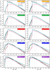 |
Fig. 2. Spectral energy distribution (continuum) of chemically homogeneously evolving stars in different evolutionary stages as marked in the colored boxes in each panel. Left panels: provide the continuum SED of the models calculated with a smooth (D = 1) wind, while the right panels depict the same for the clumped (D = 10) wind assumption. The colored lines correspond to the models with specific Mini (denoted in the top panels) and calculated assuming the same (nominal) mass-loss rate as given in Table 1. For each colored line, a black line also represents the SED of the model for the same star in the same evolutionary stages with the same clumping factor D, but assuming a mass-loss rate 100 times lower. For better visibility of the differences between the SEDs in the CHeB phase, see Fig. B1. |
Decreasing the mass-loss rates has no significant influence on the emitted radiation during most of the CHB phases. Only small differences in the emitted fluxes can be seen at wavelengths shorter than 227 Å and longer than 10 000 Å (see the differences between the colored and black lines in the left panels of Fig. 2). The same conclusion can be drawn for the clumped wind models with D = 10 (see the differences between the colored and black lines in the right panels of Fig. 2). These differences are higher and more visible in the evolutionary stages shortly before the end of CHB phase and in the CHeB phase (see the differences between the colored and black lines in the left and right panels with blue and purple boxes in Fig. 2).
The differences in the emitted fluxes between models calculated for smooth and clumped wind are very small and present mostly at the wavelengths shorter than 227 Å, regardless of the adopted Ṁ. Small differences between SEDs are also found at wavelengths longer than 10 000 Å for models in the later stages, assuming higher Ṁ (see the differences between the black and colored lines in the left panels with higher Ṁ and in the right panels with reduced Ṁ in Fig. B2).
The SEDs reveal that the radiation with frequencies higher than the H I, He I, and He II ionization limits increase both with the initial mass and during the evolution of the stars. More massive and more evolved stars emit more ionizing flux. The consequences of ionizing fluxes of chemically homogeneously evolving stars and their application will be discussed in a subsequent paper (Szécsi et al., in prep.).
4.1. Description of spectral features
To discuss the detailed spectral features, we analyzed the normalized spectra. The optical range is depicted in Figs. 3 and 4, and the spectra in the UV and infrared (IR) regions of each model are plotted in Figs. B3–B6.
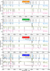 |
Fig. 3. PoWR spectra in the optical region of TWUIN stars with different Mini (see labels on the right sides of the panels) and in different CHB evolutionary phases marked by the value YS in the colored boxes. The colored lines correspond to the models calculated with mass-loss rates as given in Table 1. The black lines correspond to the models of the same stars in the same evolutionary stages, but calculated with mass-loss rates 100 times lower (i.e., reduced Ṁ). In all cases, the spectra correspond to smooth (D = 1) wind models. |
The spectra calculated with mass-loss rates taken from stellar evolution calculations and assuming a smooth wind in earlier evolutionary phases with CHB show most lines in absorption (see the colored lines in Fig. 3). These lines turn into emission in the CHeB phase, during which these stars have no hydrogen in the atmosphere (see the colored lines in the top panel in Fig. 4). This trend is also visible in the UV and IR spectra (see also the colored lines in Figs. B3 and B5 and in the top panels in Figs. B4 and B6). The spectra of these stars do not typically show any P Cygni line profiles. This is somewhat surprising, but is most likely related to the low Z of these stars.
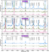 |
Fig. 4. Top panel: same as Fig. 3, but for the CHeB evolutionary phase with YS as given in Table 1. Middle and lowest panels: same as the top panel, but for clumped wind (i.e., D = 10) with nominal (i.e., higher) Ṁ (middle panel) and reduced Ṁ (lowest panel); black lines correspond to the model with smooth wind assumption. |
Synthetic spectra of models with YS = 0.25 and YS = 0.5, regardless of their initial mass, show almost exclusively absorption lines in most of the spectral regions, except for the emission line N IV λ7123 Å in the optical range (see the pink line in the panel with the green box in Fig. 3); and very weak blending lines He II λ1.86 μm and He I λ1.88 μm in the IR range (see the purple and green lines in the panels with the orange and green boxes in Fig. B5).
When the stars reach the evolutionary stage with YS = 0.75, some additional emission lines appear in the spectra of the higher-mass models (Mini = 59 M⊙ and 131 M⊙). For instance, the helium emission line He II λ4686 Å and the hydrogen emission line Hα λ6563 Å can be found in the optical spectra (see the green and blue lines in the panel with the red box in Fig. 3). In the UV spectral region, the helium emission line He II λ 1641 Å and the nitrogen line N V λ 1239 Å can be found (see the colored line in the panel with the red box in Fig. B3). In the IR part of the spectra, additional He II emission lines (e.g., He II 1.01 μm and He II 1.16 μm) can be found only in the spectra of the highest-mass model (i.e., Mini = 131 M⊙, see the blue line in the panel with the red box in Fig. B5). The model with Mini = 20 M⊙ does not show any sign of emission lines in this evolutionary phase. Even the emission line N IV λ7123 Å disappears.
At the evolutionary stage with YS = 0.98, that is to say, shortly before the end of CHB, synthetic spectra of the higher-mass models with Mini = 59 M⊙ and 131 M⊙ show more intense emission lines. In addition to the emission lines they had in the previous evolutionary phases, more He II lines in all spectral regions are now in emission (see the colored lines in the panels with the blue boxes in Fig. 3, and in Figs. B3 and B5). In the UV spectral region, a hydrogen line Lα λ1216 Å appears in emission. This line would probably be masked by interstellar absorption when observed in the local Universe; but at high redshift, provided that a sufficiently massive population of chemically homogeneously evolving stars are present, it may indeed be identifiable in the host galaxy spectra.
In addition, other He II lines as well as metal lines of C IV and O VI appear (see the colored lines in the panel with the blue box in Fig. B3). Of the N V lines, only N V λ4606 Å is detected in in absorption, every other nitrogen line is completely absent. In the IR spectral regions, more He II lines are now seen in emission (see the colored lines in the panel with the blue box in Fig. B5). Lines that were in emission in the previous evolutionary phase now become much stronger. The spectra with Mini = 20 M⊙ also show these emission lines at this evolutionary stage.
The strongest emission line in the optical spectra up to this evolutionary stage is the He II λ4686 Å line. The flux in the line center corresponds up to about twice that of the continuum (see zoom of the optical spectra in the upper panels in Fig. 5). Another strong line in the optical spectrum is a blend of He II λ6560 Å and hydrogen Hα (see zoom of the optical spectra in the lower panels in Fig. 5). The strongest line in the UV spectra is He II λ1640 Å, while in the IR, we find the strongest line to be He II λ1.01 μm and He II λ1.86 μm.
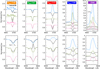 |
Fig. 5. Same as Fig. 3, but zooming in on the He II λ4686 Å line (upper panels) and Hα line blended with He II λ6560 Å line (lower panels). In the CHeB evolutionary phase, the C IV λ4657 Å line appears. |
At the CHeB stage, all models show almost only emission lines. These are much stronger than any emission line in the preceding CHB phases. In addition to the He II lines, more metal lines of C and O begin to appear (see the colored lines in the upper panels in Fig. 4 and Figs. B4 and B6). N lines are again completely absent, except for Ni V λ4606 Å, but it is very weak. The strongest lines in the optical spectrum in this evolutionary phase are the oxygen doublet O VI λλ3811, 3834 Å, the carbon line C IV λ4657 Å blended with He II λ4686 Å, and C IV λ7724 Å. Additionally, other lines are also strong, for instance, O VI λ4499 Å, O VI λ5288 Å, and O VI λ6191 Å. In the UV region the strongest lines are O VI λ1032 Å and the doublet line C IV λλ1548, 1551 Å, but also O VI λ1125 Å, O VI λ2070 Å, and He II λ1641 Å. In the IR region the strongest lines are O VI λ1.08 μm, O VI λ1.46 μm, and O VI λ1.92 μm.
We infer that chemically homogeneously evolving stars in early evolutionary phases show spectral features that are typical of weak and optically thin winds. Thus the term TWUIN star indeed applies to them. In the later evolutionary phases, however, these stars begin to exhibit spectral features that are common for stars with strong and optically thick winds. These features are typical of WR stars.
Table 3 lists the optical depths of the winds of our individual PoWR models. We defined them as the layers with a wind velocity of v > 0.1 km s−1. This is in line with the definition from Eq. (14) in Langer (1989) that we applied in Paper I, but it no longer explicitly relies on the β-law, although this law is implicitly used in the atmosphere models. We list two different optical depth scales in Table 3: τThom, which includes only the Thomson electron scattering, thereby allowing a direct comparison with the estimates made without a detailed atmosphere calculation in Paper I, while τRoss is the Rosseland mean optical depth that includes all lines and continuum opacity, which is an even more meaningful quantity for identifying optically thick regimes. We marked models with a wind optical depth of τ < 1 in both scales as TWUIN stars.
Wind optical depths from our PoWR models.
We find that all models with a reduced mass-loss rate (regardless of clumping) belong to TWUIN stars (i.e., they have a transparent wind), even in their CHeB stages. Models with nominal mass-loss rates and clumping develop an optically thick wind in their CHeB stages after they experienced the TWUIN phase during their CHB stages. Additionally, the models with high Mini (i.e., Mini = 59 and 131) have optically thick winds even in stages just before the CHeB phase (i.e., with 0.98% of He ). From this we can conclude that throughout most of their lifetimes, chemically homogeneously evolving stars at low Z that emit most of their radiation in the UV (see Sect. 6.1.1) have a transparent wind, or in other words, they are TWUIN stars. However, the existence of several optically thick lines or continua in a part of the wind is not excluded. All this is a consequence of the adopted Ṁ prescriptions in the calculations, as we discuss in the following section.
4.2. Effect of mass loss
To study the effect of mass-loss rates on the synthetic spectra, we calculated a set of models with mass-loss rates that are 100 times lower than used in the stellar evolution calculations. The other parameters remained unchanged. These models are plotted as black lines in Figs. 3, and 5, and in the top panels of Figs. 4, but also in Figs. B3, and B5, and in the top panels of Figs. B4 and B6.
Models with lower mass-loss rate yield mostly absorption-line spectra during the CHB evolutionary phases. They show only negligible emission features (see the black lines in Fig. 3 and Figs. B3 and B5). Lowering the mass-loss rate affects the strength of the lines. While those few lines that are in emission become less intense, for most of the lines that are already in absorption using the lower mass-loss rates, the absorption becomes even deeper. This illustrates that even pure absorption lines can be filled up by wind emission when applying higher Ṁ. A more prominent effect of the same origin is the change in some lines from emission to absorption (see the differences between the colored and black lines in Fig. 3 and Figs. B3 and B5).
However, some absorption lines calculated with lower mass-loss rate become less pronounced than what is expected as a general influence of lowering mass loss. A more prominent effect of the same origin (i.e., absorption lines switch to emission) can be seen, for instance, in He II λ6560 Å blended with Hα (see the first and second lower panels from the left in Fig. 5) and He II λ1.09 μm, He II λ1.28 μm, He II λ1.88 μm, and He II λ1.88 μm blended with H I lines (see the upper two panels with orange and green boxes in Fig. B5). The reason is that for the models with a higher percentage of hydrogen (more than 50%), the He II lines that are in absorption are blended with hydrogen emission lines, which are stronger. The combination of the He II absorption line and H I emission lines results in the effect we described above. For more evolved models (i.e., those that have much less or no helium at the surface), this effect is not visible.
The low mass-loss spectra of less evolved TWUIN stars (with YS = 0.28 and YS = 0.5) regardless of their mass do not show any significant differences from their high mass-loss counterparts except for the effect we described above. Thus we can conclude that in early evolutionary stages, the assumptions about mass loss in stellar evolutionary computations has a negligible effect and would not lead to predicting different observable spectra.
At the evolutionary stage YS = 0.75, the spectra with Mini = 59 and 131 M⊙ show changes in some optical lines (e.g., He II at λ4686 Å and λ6560 Å) from emission to absorption with decreasing mass-loss rate, while those with Mini = 20 M⊙ still do not show any significant difference in their spectra (see the panel with the red box in Fig. 3). A similar effect is seen in the UV and IR regions (see the panels with the red boxes in Figs. B3 and B5).
The fact that chemically homogeneously evolving stars in early evolutionary stages have weak and transparent winds is in accordance with previous studies such as Paper I. There the authors were motivated to introduce the class of TWUIN stars.
For stars in the evolutionary stage YS = 0.98, the effect of the mass loss on the spectra is more pronounced. These spectra show a few very weak emission lines, such as He II at λ4200 Å and He II λ5412 Å (see the panel with the blue box in Fig. 3). In the UV and IR spectral regions, the effect of a decreasing mass-loss rate is also visible (see the panels with the blue boxes in Figs. B3 and B5). The spectra with 20 M⊙ show the same spectral features as more massive stars in previous evolutionary stages.
The most pronounced differences appear for the latest evolutionary stage. Models with CHeB show a strong dependence on the applied mass-loss rate, particularly for the stars with Mini = 59 and 131 M⊙ (see the top panel in Fig. 4 and Figs. B4 and B6). These more evolved stars have a strong and thick wind with our default prescription, and thus decreasing the mass-loss rates has an enormous influence on the resulting spectra. While the nominal mass loss produces very strong and broad emission features, the reduced one produces much less pronounced emission lines, if any. We therefore conclude that while varying the mass-loss rates in the early evolutionary phases has no significant effect on the spectral appearance of these TWUIN stars, proper mass-loss rates for the more evolved stages where the models start to show WR-features are of uttermost importance.
4.3. Effect of clumping
From observations and theoretical considerations, we know that winds of almost all massive stars are inhomogeneous (e.g., Hamann et al. 2008; Puls et al. 2008). The absence of direct observations of chemically homogeneously evolving (TWUIN) stars also means that we do not have any observational constraint on clumping. However, we can check how wind inhomogeneities may influence the spectral appearance from a purely theoretical point of view. Using a different clumping factor D, here we study how much the spectral appearance changes when all other parameters are kept the same.
For our two sets of models, the set with the mass-loss rates as used in the stellar evolutionary models (higher Ṁ) and the other set with mass-loss rates 100 times lower (reduced Ṁ), we calculated spectra with clumping factors D = 1 (corresponding to a smooth wind) and D = 10 assuming a clumping onset in the wind.
For the models with higher mass-loss rates, the general influence of clumping on the spectral appearance is a reduction of absorption. The lines that are in emission in the smooth wind models are made much stronger by clumping. Some lines even switch from absorption to emission, for instance, the He II λ1641 Å, λ4686 Å, λ5412 Å lines and He II λ6560 Å line blended with the hydrogen Hα λ6563 Å line (see Fig. 6 and also Figs. B8 and B10).
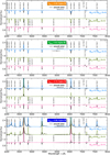 |
Fig. 6. PoWR spectra in the optical region of TWUIN stars with different Mini (see labels on the right side of the panels) and in different CHB evolutionary phases marked by the value YS in the colored boxes. The mass-loss rates are taken from the stellar evolutionary calculations (i.e., higher Ṁ). Colored lines correspond to the clumped wind models (i.e., D = 10), while the black lines correspond to the smooth wind. |
For the models with reduced mass-loss rates, spectra during the CHB phases stay almost unchanged when clumping is taken into account (see the comparison between the colored and black lines in Figs. B7, B9, and B11). This effect is reasonable because with reduced mass-loss rates the wind becomes weaker, less dense, and more transparent. Hence, introducing clumping contributes very little to the changes in optical properties of the wind.
The influence of clumping on spectral appearance is as expected. Models with the same  give similar spectra (at least the same equivalent width of the recombination lines). Therefore, if we increase clumping with the same Ṁ, the spectra react as if we had increased Ṁ. If Ṁ is low enough not to affect the recombination lines very much, we do not see much difference, which is why the low-Ṁ models do not show much difference.
The importance of clumping is more pronounced in the CHeB phase. In this stage, the winds become stronger and denser, and the contribution of clumping to the line formation becomes important. The models for CHeB stars with higher mass-loss rates show very pronounced emission lines, which become even stronger when clumping is taken into account, as shown in Fig. 7. With clumping, the dense wind becomes more transparent, and thus more radiation can escape and contribute to the line strength (see the middle panels in Fig. 4). However, the models with reduced mass-loss rates remain, even in this evolutionary stage, almost unchanged when clumping is taken into account (see the lowest panel in Fig. 4). A similar effect is seen in the UV and IR regions (see the middle and lowest panels in Figs. B4 and B6).
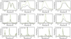 |
Fig. 7. Influence of clumping on the line strength. Emission lines in the optical (upper panels), the UV (middle panels), and the IR (lower panels) regions of the model with Mini = 131 M⊙ in the CHeB evolutionary phase (mass-loss rate of log(Ṁ/M⊙/yr = −4.23)). X-axis is centered around the wavelength indicated by the key legend (e.g., He II 4686 means He II λ4686 Å). Green lines corresponds to clumped wind models with D = 10, and black lines to smooth wind models with D = 1. |
5. Spectral classification
We classified our model spectra according to the commonly used Morgan–Keenan spectroscopic classification scheme. We give a detailed description of this classification scheme in the context of hot massive stars in Appendix A. We report our findings summarized in Table 4, and discuss some details below.
Spectral classification of our stellar models.
5.1. TWUIN stars are very hot O stars
Most of our spectra that show almost no emission lines, that is, the stellar models that have been designated as TWUIN stars in Paper I, are assigned to class O 4 or earlier. This means that they are very early O-type giants or supergiants because the logarithm of the ratio of He I λ4473 Å to He II λ4543 Å, which is being smaller than −0.6, causes them to belong at least to type O 4 (Mathys 1988), and in the absence of nitrogen lines, we cannot distinguish between earlier classes (as done, e.g., in Walborn et al. 2002). The ratio of these helium lines is usually around −1.5 or lower. All we can safely say for these stars therefore is that they are of class O 4 or earlier.
Luminosity classes for the spectra that are consistent with classes earlier than O 4 type (marked as < O 4 in Table 4) are defined based on the nature of the He II λ4686 Å line. If it is found in emission, the spectrum is classified as a supergiant (i.e., luminosity class I). If it is found in weak absorption (i.e., the logarithm of the absolute value of the equivalent width is lower than 2.7, cf. Mathys 1988), the spectrum is classified as a giant (i.e., luminosity class III), and if it is strongly in absorption, a dwarf (i.e., luminosity class V).
We find late-O type stars, that is, O 5 to O 9.5, only among the lowest mass models (with Mini = 20 M⊙). As for their luminosity classes, we applied two criteria: one for those earlier than O 8, as explained above, and another for those between O 8.5−O 9.5 (cf. Appendix A). This other criterion is provided by Conti & Alschuler (1971) and is based on the equivalent width ratio of the lines Si IV λ4090 Å and He I λ4143 Å (but see also Martins 2018). With this, our spectra of a 20 M⊙ star are assigned to dwarf (V) at the ZAMS and to giant (III) in the middle of the MS phase. However, this distinction seems to be an artifact of using two different criteria for those earlier and later than O 8. As Fig. 1 and Table 1 attest, the radius of the 20 M⊙ model does not change significantly between the phases YS = 0.28 and YS = 0.5. The luminosity does change, however, showing that the conventional nomenclature associated with luminosity classes (giant, dwarf, etc.) may not always be very meaningful in accounting for the radial size of a star.
We did not find any of our spectra to be consistent with the O f subclass (Crowther et al. 1995; Crowther & Walborn 2011) because the defining feature of this subclass, the line N III λ4640 Å, is completely absent in all our spectra. The O f subclass practically means that the star has a fairly strong wind; therefore galactic early-type stars tend to have it. It is not surprising, however, that our low-metallicity stars with weak winds do not show this feature.
Some of our < O 4 stars are really hot. Tramper et al. (2014) investigated ten low-metallicity (down to 0.1 Z⊙) O-type stars and found the hottest to be Teff = 45 kK, while our hottest O-type object has Teff = 85 kK. The detection of a very hot, early-O type star at low metallicity without an IR-excess would therefore mean that this source is a strong candidate for a star resulting from chemically homogeneous evolution. We refer to our Sect. 6.1, where we compare one of our < O 4 type spectra to a regular O-type stellar spectra from the literature.
5.2. TWUIN stars turn into Wolf–Rayet stars in the CHeB phase
The term Wolf–Rayet stars refers to a spectral class, based on broad and bright emission lines that are observed in the optical region. As briefly described in Sect. 1, authors working on stellar evolution sometimes refer to objects that are hot and (more or less) hydrogen-deficient as WR stars as well. From an evolutionary point of view, the surface of a massive star can become hydrogen-poor because of the (partial) loss of the hydrogen-rich envelope either by Roche-lobe overflow (a scenario originally suggested by Paczyński 1967), or by stellar winds (Conti 1975). A third option that can lead to a hydrogen-deficient surface composition is internal mixing (e.g., due to rotation, as in the present work). Nonetheless, the fact that a stellar model surface is hydrogen poor does not necessarily mean that its wind is optically thick (as shown in Sect. 6 of Paper ). It does not mean either that broad emission lines develop (as shown by our CHB spectra), although this may occur (as shown by our CHeB spectra). Below we discuss the spectral classes of the latter case.
All our spectra of the CHeB phase show features typical for WR stars of the WO type: strong C IV λ5808 Å, O V λ5590 Å, and O VI λ3818 Å in emission. We classify these objects according to criteria in Table 3 of Crowther et al. (1998). There are two main criteria, a primary and a secondary. We find that these two sometimes do not provide the same class. In this case, we mention the secondary classification in square brackets in our Table 4.
We find that nitrogen lines are almost completely absent. The line N V λ4606 Å is sometimes present, most of the time in absorption. When it is in emission, its equivalent width never increases above 0.3 Å, which means that it is very weak. Other lines typical for WN stars (Smith et al. 1996) such as N III λ4640 Å and N IV λ4057 Å, are not found in any of our spectra. The almost complete absence of N-lines may make a future observer consider such a star to be some other type, certainly not WN.
Thus we conclude that after first producing very hot early-O type stars during the CHB phase, chemically homogeneous evolution leads to WO type stars during the CHeB phase. We recall that the CHeB lifetime is about 10% as long as the CHB lifetime. Therefore, in a population of chemically homogeneously evolving stars, we expect to find ten times more hot early-O stars than WO stars.
6. Discussion
6.1. Comparison to synthetic spectra from the literature
6.1.1. O-type spectra
We compared one of our absorption line spectra to a typical O-type spectra in the literature. In particular, we compared our model labeled T-8 in Table 1 (with clumping and nominal mass-loss rate), and a model spectrum of an O 3 star taken from the PoWR SMC OB model grid (see Hainich et al. 2019) database1 (see Fig. 8) corresponding to the composition of the SMC (ZSMC ∼ 0.2 M⊙). The parameters of the SMC O 3 model are Teff = 50 kK, log(L*/L⊙) = 5.52, log(Ṁ/M⊙/yr = −5.9, log(g cm−1 s−2) = 4.4, and D = 10. We note that the main differences between the two models are (i) the metallicity (ours is about ten times lower, but the He abundance is almost the same) and (ii) the surface temperature (ours is 69 kK). An effect of smoothing and broadening the lines due to fast rotation is taken into account (see Sect. 4) for both models assuming the same rotational velocity, which corresponds to the T-8 model (see Table 1).
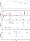 |
Fig. 8. Comparison of one of our representative O 3 III spectra (i.e., the TWUIN T-8 model, see Table 1) to an O 3 synthetic star from the literature. Both stars are placed at the same distance of 10 pc. An effect of line broadening due to fast rotation is taken into account, as described in Sect. 4 assuming the same rotational velocity, which corresponds to the T-8 model. See Sect. 6.1 for more details. |
From comparing the SEDs of both stars placed at the same distance of 10 pc (see the top panel in Fig. 8) we can infer that the amount of emitted far- and extreme UV ionizing radiation increases particularly at shorter wavelengths (around the H I ionization edge). This is consistent with the fact that our model has a higher surface temperature. Another effect that may lead to higher UV flux is that there is less line blanketing at low metallicity, therefore less flux is redistributed to longer wavelengths.
For the spectral features, we can infer the following. In the optical region, the SMC O 3 spectrum shows the C IV λλ5801, 5812 Å lines, while in the TWUIN T-8 model, we do not find any metal lines. In the UV region, the SMC O 3 spectra also show very strong metal lines (e.g., the doublet O VI λλ1032, 1038 Å, the doublet N V λλ1239, 1243 Å, O V λ1371 Å, and the doublet N IV λλ1548, 1551 Å) that are not present in the TWUIN T-8 model spectra. This is expected because the TWUIN star models have very low metallicity.
He II lines are in very strong emission in the TWUIN T-8 model spectra (e.g., He II λ1641 Å, He II λ4687 Å, and He II λ6562 Å), while in the SMC O 3 spectra, these lines are in absorption. This is consistent with the fact that the TWUIN model has a high surface helium abundance (YS ∼ 0.5). On the other hand, He I lines are not present in the TWUIN T-7 model spectra, while in SMC O 3, they are visible (see the He I λ5877 Å, He I λ7065 Å, and He I λ3888 Å lines in Fig. 8).
6.1.2. WO-type spectra
We compared our emission line spectra to a typical WO-type spectra from the literature. Comparing our models to a WO star model was difficult because no analyses of observations of WO stars exist with the metallicity we study here, and, consequently, no models exist either. For somewhat higher metallicities such as ZSMC, very few models have ever been calculated. Here we used a model from Shenar et al. (2016), which was applied for the analysis of the SMC binary star AB 8 with the following model parameters: Teff = 141 kK, log(L*/L⊙) = 6.15, log(Ṁ/M⊙/yr = −4.8, v∞ = 3700 km s−1, log g(cm−1 s−2) = 5.4, and D = 40. These parameters are similar to those of our T-10 model (see Table 1) with clumping and nominal mass-loss rate.
The comparison is shown in Fig. 9. For both models rotation is taken into account assuming the same rotational velocity, which corresponds to the T-10 model (see Table 1). The T-10 model is somewhat more luminous. Both models have the same beta (i.e., β = 1), and similar mass-loss rates and log g. The mass-loss rates of both models are relatively high, but we do expect the Z-dependency to drop for WO stars because their atmospheres are enriched with fusion products that are not related to the initial metallicity, and these products contribute to the driving of their winds. Moreover, the WO star in the SMC seems to be much more luminous than the Galactic WO stars, which increase their mass-loss rate compared to other WO stars.
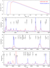 |
Fig. 9. Same as Fig. 8, but comparing our WO 1 spectra (i.e., TWUIN T-10 model, see Table 1) to an SMC WO 4 synthetic spectrum from Shenar et al. (2016). |
The main differences between the two models are (i) the surface temperature (ours is 138 kK), (ii) the terminal velocity (ours is 1000 km s−1), (iii) the clumping factor (ours is 10), and (iv) the metallicity and element ratios (see the mass fractions in Table 1). The mass-fraction of the WO 4 model are He = 0.399, C = 3 × 10⁻¹, O = 3 × 10⁻¹, and Fe = 6 × 10⁻⁴. In the WO 4 model, N was not included, while in the T-10 model it is. For both models, H is not included. The T-10 model has about twice as much, somewhat less C, by more than two orders of magnitude less O, and by more than one order of magnitude fewer iron group elements.
The difference in SED (see the top panel in Fig. 9) can be attributed to the different Fe abundances in the models. The Fe abundance in the WO star model is more than an order of magnitude higher than in our T-10 model, causing substantial absorption and re-emission of UV photons in the visual part (line blanketing). The difference in the spectral line shapes can mainly be attributed to differences in v∞, which is more than a factor three larger in the WO model. Finally, the large differences in the strength of some spectral lines is a result of differences in two things: the abundances, and the so-called “transformed radii” Rt, which represent an integrated emission measure in the wind (see Eq. (1) in Hamann et al. 2006). The SMC WO model has a higher Rt value, and hence overall weaker spectral lines. Although the spectra of these models differ significantly, they do predict similar lines to appear in the spectrum.
To conclude, the different environment and formation history of chemically homogeneously evolving stars could mean that they appear somewhat different than the SMC WO component at their evolved phases. Their exact appearance would depend on parameters such as the terminal velocity, which was fixed in our study. Regardless of this uncertainty, however, we find that so-called TWUIN stars appear as WO stars in their evolved phases.
6.2. Validity of our model assumptions
Our wind models and emergent spectra are theoretical predictions based on current knowledge of stellar evolution and stellar wind modeling. However, they are also subject to several assumptions.
The radial wind velocities in our models were assumed to follow the β-law in Eq. (5). Although there exist several calculations of the wind velocity law that take into account acceleration of matter by scattered and absorbed radiation either in an approximate way using force multipliers (e.g., Castor et al. 1975; Abbott 1980; Pauldrach et al. 1986) or in a more exact way using detailed radiative transfer (e.g., Abbott 1982; Gräfener & Hamann 2005; Pauldrach et al. 2012; Krtička & Kubát 2010, 2017; Sander et al. 2017), the β-velocity law became a standard assumption in modeling stellar wind spectra. Using a free parameter β allows finding a velocity law that fits the observations best, regardless of the consistency of such a result. As discussed by Krtička et al. (2011), the β-velocity law is a good approximation to consistent hydrodynamical calculations, but a better and more exact fit can be obtained using Legendre polynomials. In any case, using the β-velocity law is a reasonable first approximation.
We also had to assume a mass-loss rate. This was done by taking the mass-loss rates that were assumed in the stellar evolutionary models. As explained in Sect. 2.1, the evolutionary models assumed a mass-loss rate following certain recipes. The recipe of Vink et al. (2000, 2001) in Eq. (1) was derived from atmosphere simulations that used a detailed treatment of a full line list for a fixed velocity law. The recipe of Hamann et al. (1995) given in Eq. (2) was, on the other hand, based on observed spectra of WR stars. Nonetheless, these prescriptions may not be valid for TWUIN stars. To ensure that we understand the consequences of using them anyway, we therefore tested the effect of decreasing the mass loss by 100, to be consistent with the findings of Hainich et al. (2015, cf. our Table 2). The results of this test in the context of line formation was reported in Sect. 4.2.
As chemically homogeneously evolving stars are generally fast rotators (∼0.6 vcrit), this may have some as yet unexplored effect on their wind structures (Owocki et al. 1996). However, this would require detailed hydrodynamical calculations in at least 2D, which are beyond the scope of this paper. We accounted for the spectral imprint of fast rotation by performing a flux convolution of the emergent spectrum with a rotation profile.
Here we only studied the spectra of single stars, but a large fraction of massive stars are born in close binary systems and thus undergo interaction with a companion during the evolution at some point (e.g., Paczyński 1967; Sana et al. 2012; Götberg et al. 2017). However, the ratio of binary stars versus single stars is unknown at the metallicity we study, and it may be quite different from the Galactic case (e.g., because the stability of the collapsing star-forming cloud may be influenced by its metallicity). For example, TWUIN stars in a close binary orbit have been suggested to be the stellar progenitors of compact object mergers, explaining the origin of gravitational waves (Marchant et al. 2016, 2017). How such an interaction with a companion influences the spectral appearance remains to be studied.
6.3. Future research on TWUIN stars – theory
Taking the same mass-loss rate as was assumed when computing the evolution makes our spectral predictions consistent with evolutionary models. However, in the absence of actual observations of TWUIN stars, the question is whether such a star can have a wind at all. Testing this can be done similarly to how it was done by Krtička & Kubát (2014) for the case of winds with non-solar CNO abundances. Although this test is computationally expensive and goes beyond the scope of this work, here we summarize the basic idea, as well as the results we may expect from such a test, as a motivation for future work.
As described, we assumed that the wind structure of all TWUIN stars can be described by a β-law (e.g., Puls et al. 2008), motivated by hydrodynamical consistent calculations for Galactic WN stars, for example (Gräfener & Hamann 2008). Additionally, we assumed input parameters (β, v∞) that are typical for hot massive O-type stars and WR stars at 0.2…1 Z⊙. All this may not hold for extremely low-metallicity environments; and the issue is further complicated by the observed steep metallicity dependence of the mass loss found by Hainich et al. (2015) as well as by the so-called “weak wind problem” (see, e.g., Martins et al. 2005; Marcolino et al. 2009; Huenemoerder et al. 2012).
One way to validate the assumptions we used in this work would be hydrodynamical simulations of the wind and its structure. This has been done for Galactic massive O stars in Krtička & Kubát (2017) and for a few WR stars in Gräfener & Hamann (2008). Although expensive, such simulations for the models presented in this work could provide essential information on how valid our spectrum predictions are.
For example, if atmosphere models based on hydrodynamic simulations point to different values for β, Ṁ, or v∞, this will influence the predicted line strengths in our spectra and thus lead to assigning different spectral classes for these stars. The models may even show that the β-law as such is not applicable at all in this regime or that these stars, at least during some parts of their evolution, might not have winds at all. Thus, future studies in this direction are sorely needed.
As for metallicity, here we only applied one set of stellar evolutionary models, all computed with Zini = 0.02 Z⊙. However, chemically homogeneous evolution is predicted to occur at various sub-solar metallicities (see, e.g., Brott et al. 2011). Although its prevalence is expected to be larger at lower metallicity (see Sect. 10.4 of Paper 1), it is nonetheless an important future research direction to study the spectra of chemically homogeneously evolving stars up to at least ZSMC.
6.4. Future research on TWUIN stars – observations
It is essential to obtain observational samples of metal-poor massive stars to test our theories. Ideally, we would need an extensive spectral catalog of about 50–100 massive stars at metallicities lower than 0.1 Z⊙. This task seems challenging, but not at all impossible with the most modern observing facilities and the next-generation telescopes coming up. For example, ESO’s MUSE spectrograph can take optical spectra of several dozen massive stars in local-group galaxies (Castro et al. 2018), while systematic studies of these spectra (including spectral classification and determination of mass-loss rates) could be made with advanced tools (e.g., Hillier & Miller 1998; Puls et al. 2005; Gustafsson et al. 2008; Kamann et al. 2013; Tramper et al. 2013; Ramachandran et al. 2018).
Until we obtain a comprehensive census of individual massive stars at low metallicity, we may compare our predictions to observed populations of massive stars. Such a comparison of our model predictions to unresolved observed features of massive star populations in the dwarf galaxy I Zwicky 18 (Kehrig et al. 2015, 2016) is planned in a subsequent work.
Another interesting application of our spectra might be made in the context of the reionization history of the Universe. It has been suggested that massive stars, and especially chemically homogeneous evolution, may be important for this process (e.g., Eldridge & Stanway 2012), as WR-like emission bumps are often not found in the spectra of high-redshift galaxies. We note that our spectral models suggests that TWUIN stars are indeed not expected to show prominent emission lines because their winds are rather weak. Thus, these stars’ contribution to the reionization epoch should also be investigated in the future.
7. Summary and conclusions
We studied the spectral appearance of chemically homogeneously evolving stars, as predicted by evolutionary model sequences of fast-rotating massive single stars with low metallicity. To compute the spectra, we employed the NLTE model stellar atmosphere and stellar wind code PoWR. We predicted detailed spectra for selected stars from three evolutionary models: those with initial masses 20 M⊙, 59 M⊙, and 131 M⊙. Various evolutionary stages were studied (comprising the CHB and CHeB phases). The stellar parameters effective temperature, luminosity, mass, and chemical composition were taken from the evolutionary models. Wind models and their spectra were calculated for fixed values of the terminal velocity and velocity law. We tested the influence of two of the most uncertain assumptions in stellar wind modeling, mass-loss rate and clumping. The model spectra were classified according to the Morgan–Keenan spectroscopic classification scheme. Our main findings are summarized below.
-
Our models in early evolutionary phases have weak and optically thin winds, while in later phases, these stars exhibit stronger and optically thick winds. This is consistent with earlier studies (see Paper I, which established that in the early phases, these objects should be called TWUIN stars), and is a consequence of the adopted Ṁ prescription. When adopting a reduced mass-loss rate, we find only a few weak emission lines in the spectra even in the most evolved phases.
-
The maximum of the emitted radiation is in the far- and extreme UV region. The emitted radiation in the He II continuum increases both with Mini and the evolutionary status, later stages having higher emissions. The total emitted flux is not very sensitive to variations of either the mass-loss rate or clumping.
-
In earlier evolutionary phases with 50% of hydrogen or more in the atmosphere, most of our spectra, regardless of their Mini, almost exclusively show absorption lines. This is true for the whole spectral region. More emission lines start to appear in later evolutionary phases, shortly before the end of the CHB phase. In the CHeB phase almost all lines are found in emission. In particular, the helium emission lines are strong and very characteristic for evolved stars. Their line strengths increase with higher helium abundance.
-
Our models predict that lower mass-loss rates than those adopted from the evolutionary calculations have a negligible effect on the emergent spectra of the TWUIN star models in early evolutionary phases. More pronounced influence on spectral appearance is seen in later evolutionary phases with more helium in the atmosphere, especially in the CHeB phase.
-
The assumed clumped wind has no significant influence on the predicted TWUIN spectra in earlier evolutionary phases. The spectra of higher-mass models in later evolutionary phases are, on the other hand, sensitive to clumping. Reducing the mass-loss rate cancels out this sensitivity, however, that is, model spectra with reduced mass-loss rates remain almost unchanged when a clumped wind is assumed, even in late evolutionary phases.
-
Our TWUIN model spectra are assigned to spectral class O 4 or earlier. Nitrogen lines are almost completely absent. TWUIN O-type stars are predicted to be much hotter than the O-type stars that have been observed spectroscopically so far (down to 0.1 Z⊙). Thus, the detection of a very hot star without almost any metal lines but with strong He II emission lines that is consistent with some very early-O type giant or supergiant would be a strong candidate for a star resulting from chemically homogeneous evolution.
-
In later evolutionary phases, most of our model spectra are assigned to the WO-type spectral class. Nitrogen lines are almost completely absent in this late phase as well. Thus, chemically homogeneous evolution first leads to very hot early-type O stars (TWUIN stars) and then, for the last ≲10% of the evolution, to Wolf–Rayet stars of type WO.
-
The fact that chemically homogeneously evolving stars only develop emission lines during their CHeB phase, but have only absorption lines during their long lived CHB phase (when they are TWUIN stars), suggests that these stars may have contributed to the reionization of the Universe. Observations of high-redshift galaxies typically show that an intensive ionizing source is present that produces almost no WR-like emission bumps in the galactic spectra. Some populations of TWUIN stars may be this source.
Single stars with chemically homogeneous evolution may be the progenitors of long-duration gamma-ray bursts and type Ic supernovae, as shown, for example, by Yoon et al. (2006) and Szécsi (2016, Chapter 4). In a close binary system, they may lead to two compact objects that eventually merge, giving rise to detectable gravitational wave emission (Marchant et al. 2016, 2017). Our choice of metallicity was indeed motivated by the fact that at this metallicity, binary models predict a high rate of gravitational-wave-emitting mergers.
Our test with the two mass-loss rate values indicates that even if the mass-loss rate turns out to be much lower than what is applied in the evolutionary models during the CHB phase, and indeed even if some of these stars turn out not to have winds at all, our conclusions about the absorption-like spectra will remain the same. In the CHeB phase, the mass-loss rate plays an important role; we suggest carrying out hydrodynamic simulations of the wind structure for these stars, to enable constraining their mass-loss rates and thereby to investigate their spectral appearance further.
As a result of the lack of spectroscopic observations of individual massive stars with metallicity below 0.1 Z⊙, we were unable to compare our spectra with observations of any stars that may be of similar nature. The main purpose of our work is indeed to motivate future observing campaigns aiming at low-metallicity star-forming galaxies such as Sextant A or I Zwicky 18.
Acknowledgments
This research was supported by grant 16-01116S (GA ČR). The Astronomical Institute Ondřejov is supported by the project RVO:67985815. D. Sz. is grateful for the relevant discussion with G. Gräfener and N. Langer, as well as to Á. Szabó, as usual. A.A.C.S. is supported by the Deutsche Forschungsgemeinschaft (DFG) under grant HA 1455/26 and would like to thank STFC for funding under grant number ST/R000565/1. TS acknowledges funding from the European Research Council (ERC) under the European Union’s DLV-772225-MULTIPLES Horizon 2020 research and innovation program.
References
- Abbott, D. C. 1980, ApJ, 242, 1183 [NASA ADS] [CrossRef] [Google Scholar]
- Abbott, D. C. 1982, ApJ, 259, 282 [NASA ADS] [CrossRef] [Google Scholar]
- Abbott, B. P., Abbott, R., Abbott, T. D., et al. 2016, ApJ, 818, L22 [Google Scholar]
- Abbott, B. P., Abbott, R., Abbott, T. D., et al. 2017, Phys. Rev. Lett., 118, 221101 [NASA ADS] [CrossRef] [PubMed] [Google Scholar]
- Abel, T., Bryan, G., & Norman, M. 2002, Science, 295, 93 [NASA ADS] [CrossRef] [PubMed] [Google Scholar]
- Annibali, F., Cignoni, M., Tosi, M., et al. 2013, AJ, 146, 144 [NASA ADS] [CrossRef] [Google Scholar]
- Bouret, J.-C., Lanz, T., Hillier, D. J., et al. 2015, MNRAS, 449, 1545 [NASA ADS] [CrossRef] [Google Scholar]
- Brott, I., de Mink, S. E., Cantiello, M., et al. 2011, A&A, 530, A115 [NASA ADS] [CrossRef] [EDP Sciences] [Google Scholar]
- Camacho, I., Garcia, M., Herrero, A., & Simón-Díaz, S. 2016, A&A, 585, A82 [NASA ADS] [CrossRef] [EDP Sciences] [Google Scholar]
- Cantiello, M., Yoon, S.-C., Langer, N., & Livio, M. 2007, A&A, 465, L29 [NASA ADS] [CrossRef] [EDP Sciences] [Google Scholar]
- Castor, J. I., Abbott, D. C., & Klein, R. I. 1975, ApJ, 195, 157 [NASA ADS] [CrossRef] [Google Scholar]
- Castro, N., Crowther, P. A., Evans, C. J., et al. 2018, A&A, 614, A147 [NASA ADS] [CrossRef] [EDP Sciences] [Google Scholar]
- Choudhury, T. R., & Ferrara, A. 2007, MNRAS, 380, L6 [NASA ADS] [Google Scholar]
- Conti, P. S. 1975, Mem. Soc. Roy. Sci. Liege, 9, 193 [Google Scholar]
- Conti, P. S., & Alschuler, W. R. 1971, ApJ, 170, 325 [NASA ADS] [CrossRef] [Google Scholar]
- Conti, P. S., & Frost, S. A. 1977, ApJ, 212, 728 [NASA ADS] [CrossRef] [Google Scholar]
- Conti, P. S., & Leep, E. M. 1974, ApJ, 193, 113 [NASA ADS] [CrossRef] [Google Scholar]
- Crowther, P. A., & Hadfield, L. J. 2006, A&A, 449, 711 [NASA ADS] [CrossRef] [EDP Sciences] [Google Scholar]
- Crowther, P. A., & Walborn, N. R. 2011, MNRAS, 416, 1311 [NASA ADS] [CrossRef] [MathSciNet] [Google Scholar]
- Crowther, P. A., Hillier, D. J., & Smith, L. J. 1995, A&A, 293, 172 [NASA ADS] [Google Scholar]
- Crowther, P. A., De Marco, O., & Barlow, M. J. 1998, MNRAS, 296, 367 [NASA ADS] [CrossRef] [Google Scholar]
- Cui, Z., Wang, Z., Zhu, C., et al. 2018, PASP, 130, 084202 [NASA ADS] [CrossRef] [Google Scholar]
- Davies, B., Kudritzki, R.-P., Gazak, Z., et al. 2015, ApJ, 806, 21 [NASA ADS] [CrossRef] [Google Scholar]
- de Mink, S. E., & Mandel, I. 2016, MNRAS, 460, 3545 [NASA ADS] [CrossRef] [Google Scholar]
- de Mink, S. E., Cantiello, M., Langer, N., et al. 2009, A&A, 497, 243 [NASA ADS] [CrossRef] [EDP Sciences] [Google Scholar]
- Eldridge, J. J., & Vink, J. S. 2006, A&A, 452, 295 [NASA ADS] [CrossRef] [EDP Sciences] [Google Scholar]
- Eldridge, J. J., & Stanway, E. R. 2012, MNRAS, 419, 479 [NASA ADS] [CrossRef] [Google Scholar]
- Friend, D. B., & Abbott, D. C. 1986, ApJ, 311, 701 [NASA ADS] [CrossRef] [Google Scholar]
- Garcia, M., Herrero, A., Najarro, F., Lennon, D. J., & Urbaneja, M. A. 2014, ApJ, 788, 64 [NASA ADS] [CrossRef] [Google Scholar]
- Götberg, Y., de Mink, S. E., & Groh, J. H. 2017, A&A, 608, A11 [NASA ADS] [CrossRef] [EDP Sciences] [Google Scholar]
- Gräfener, G., & Hamann, W.-R. 2005, A&A, 432, 633 [NASA ADS] [CrossRef] [EDP Sciences] [Google Scholar]
- Gräfener, G., & Hamann, W.-R. 2008, A&A, 482, 945 [NASA ADS] [CrossRef] [EDP Sciences] [Google Scholar]
- Gräfener, G., Koesterke, L., & Hamann, W.-R. 2002, A&A, 387, 244 [NASA ADS] [CrossRef] [EDP Sciences] [Google Scholar]
- Gustafsson, B., Edvardsson, B., Eriksson, K., et al. 2008, A&A, 486, 951 [NASA ADS] [CrossRef] [EDP Sciences] [Google Scholar]
- Hainich, R., Pasemann, D., Todt, H., et al. 2015, A&A, 581, A21 [Google Scholar]
- Hainich, R., Oskinova, L. M., Shenar, T., et al. 2018, A&A, 609, A94 [NASA ADS] [CrossRef] [EDP Sciences] [Google Scholar]
- Hainich, R., Ramachandran, V., Shenar, T., et al. 2019, A&A, 621, A85 [NASA ADS] [CrossRef] [EDP Sciences] [Google Scholar]
- Hamann, W.-R., & Gräfener, G. 2003, A&A, 410, 993 [NASA ADS] [CrossRef] [EDP Sciences] [Google Scholar]
- Hamann, W.-R., & Gräfener, G. 2004, A&A, 427, 697 [NASA ADS] [CrossRef] [EDP Sciences] [Google Scholar]
- Hamann, W.-R., & Koesterke, L. 1998, A&A, 335, 1003 [NASA ADS] [Google Scholar]
- Hamann, W.-R., Koesterke, L., & Wessolowski, U. 1995, A&A, 299, 151 [NASA ADS] [Google Scholar]
- Hamann, W.-R., Gräfener, G., & Liermann, A. 2006, A&A, 457, 1015 [NASA ADS] [CrossRef] [EDP Sciences] [Google Scholar]
- Hamann, W. R., Feldmeier, A., & Oskinova, L. M. 2008, Clumping in Hot-star Winds [Google Scholar]
- Herrero, A., Garcia, M., Puls, J., et al. 2012, A&A, 543, A85 [NASA ADS] [CrossRef] [EDP Sciences] [Google Scholar]
- Hillier, D. J., & Miller, D. L. 1998, ApJ, 496, 407 [NASA ADS] [CrossRef] [Google Scholar]
- Hubeny, I., & Mihalas, D. 2014, Theory of Stellar Atmospheres (Princeton: Princeton University Press) [Google Scholar]
- Huenemoerder, D. P., Oskinova, L. M., Ignace, R., et al. 2012, ApJ, 756, L34 [NASA ADS] [CrossRef] [Google Scholar]
- Inserra, C., Pastorello, A., Turatto, M., et al. 2013, A&A, 555, A142 [NASA ADS] [CrossRef] [EDP Sciences] [Google Scholar]
- Kamann, S., Wisotzki, L., & Roth, M. M. 2013, A&A, 549, A71 [NASA ADS] [CrossRef] [EDP Sciences] [Google Scholar]
- Kehrig, C., Pérez-Montero, E., Vílchez, J. M., et al. 2013, MNRAS, 432, 2731 [NASA ADS] [CrossRef] [Google Scholar]
- Kehrig, C., Vílchez, J. M., Pérez-Montero, E., et al. 2015, ApJ, 801, L28 [NASA ADS] [CrossRef] [Google Scholar]
- Kehrig, C., Vílchez, J. M., Pérez-Montero, E., et al. 2016, MNRAS, 459, 2992 [NASA ADS] [CrossRef] [Google Scholar]
- Krtička, J., & Kubát, J. 2010, A&A, 519, A50 [NASA ADS] [CrossRef] [EDP Sciences] [Google Scholar]
- Krtička, J., & Kubát, J. 2014, A&A, 567, A63 [NASA ADS] [CrossRef] [EDP Sciences] [Google Scholar]
- Krtička, J., & Kubát, J. 2017, A&A, 606, A31 [NASA ADS] [CrossRef] [EDP Sciences] [Google Scholar]
- Krtička, J., Owocki, S. P., & Meynet, G. 2011, A&A, 527, A84 [NASA ADS] [CrossRef] [EDP Sciences] [Google Scholar]
- Kubát, J., Puls, J., & Pauldrach, A. W. A. 1999, A&A, 341, 587 [NASA ADS] [Google Scholar]
- Lamb, J. B., Oey, M. S., Segura-Cox, D. M., et al. 2016, ApJ, 817, 113 [NASA ADS] [CrossRef] [Google Scholar]
- Lamers, H. J. G. L. M., Snow, T. P., & Lindholm, D. M. 1995, ApJ, 455, 269 [NASA ADS] [CrossRef] [Google Scholar]
- Lamers, H., & Cassinelli, J. 1999, Introduction to Stellar Winds (Cambridge University Press) [CrossRef] [Google Scholar]
- Langer, N. 1989, A&A, 210, 93 [NASA ADS] [Google Scholar]
- Levesque, E. M., Kewley, L. J., Berger, E., & Zahid, H. J. 2010, AJ, 140, 1557 [NASA ADS] [CrossRef] [Google Scholar]
- Lunnan, R., Chornock, R., Berger, E., et al. 2013, ApJ, 771, 97 [NASA ADS] [CrossRef] [Google Scholar]
- Ma, Q., Maio, U., Ciardi, B., & Salvaterra, R. 2017, MNRAS, 472, 3532 [NASA ADS] [CrossRef] [Google Scholar]
- Mandel, I., & de Mink, S. E. 2016, MNRAS, 458, 2634 [NASA ADS] [CrossRef] [Google Scholar]
- Marchant, P., Langer, N., Podsiadlowski, P., Tauris, T. M., & Moriya, T. J. 2016, A&A, 588, A50 [NASA ADS] [CrossRef] [EDP Sciences] [Google Scholar]
- Marchant, P., Langer, N., Podsiadlowski, P., et al. 2017, A&A, 604, A55 [NASA ADS] [CrossRef] [EDP Sciences] [Google Scholar]
- Marcolino, W. L. F., Bouret, J.-C., Martins, F., et al. 2009, A&A, 498, 837 [NASA ADS] [CrossRef] [EDP Sciences] [Google Scholar]
- Martayan, C., Frémat, Y., Hubert, A.-M., et al. 2007, A&A, 462, 683 [NASA ADS] [CrossRef] [EDP Sciences] [Google Scholar]
- Martins, F. 2018, A&A, 616, A135 [NASA ADS] [CrossRef] [EDP Sciences] [Google Scholar]
- Martins, F., Schaerer, D., Hillier, D. J., et al. 2005, A&A, 441, 735 [NASA ADS] [CrossRef] [EDP Sciences] [Google Scholar]
- Massey, P., Neugent, K. F., & Morrell, N. 2015, ApJ, 807, 81 [NASA ADS] [CrossRef] [Google Scholar]
- Mathys, G. 1988, A&AS, 76, 427 [NASA ADS] [Google Scholar]
- Matthee, J., Sobral, D., Gronke, M., et al. 2018, A&A, 619, A136 [NASA ADS] [CrossRef] [EDP Sciences] [Google Scholar]
- McConnachie, A. W. 2012, AJ, 144, 4 [NASA ADS] [CrossRef] [Google Scholar]
- Mihalas, D. 1978, Stellar Atmospheres, 2nd ed. (San Francisco: W. H. Freeman and Co.) [Google Scholar]
- Modjaz, M., Kewley, L., Bloom, J. S., et al. 2011, ApJ, 731, L4 [NASA ADS] [CrossRef] [Google Scholar]
- Mokiem, M. R., de Koter, A., Evans, C. J., et al. 2006, A&A, 456, 1131 [NASA ADS] [CrossRef] [EDP Sciences] [Google Scholar]
- Nugis, T., & Lamers, H. 2000, A&A, 360, 227 [NASA ADS] [Google Scholar]
- Owocki, S. P., Cranmer, S. R., & Gayley, K. G. 1996, ApJ, 472, L115 [NASA ADS] [CrossRef] [Google Scholar]
- Paczyński, B. 1967, Acta Astron., 17, 355 [NASA ADS] [Google Scholar]
- Pauldrach, A., Puls, J., & Kudritzki, R. P. 1986, A&A, 164, 86 [NASA ADS] [Google Scholar]
- Pauldrach, A. W. A., Vanbeveren, D., & Hoffmann, T. L. 2012, A&A, 538, A75 [NASA ADS] [CrossRef] [EDP Sciences] [Google Scholar]
- Puls, J., Urbaneja, M. A., Venero, R., et al. 2005, A&A, 435, 669 [NASA ADS] [CrossRef] [EDP Sciences] [Google Scholar]
- Puls, J., Vink, J., & Najarro, F. 2008, A&ARv, 16, 209 [NASA ADS] [CrossRef] [EDP Sciences] [Google Scholar]
- Quimby, R. M., Kulkarni, S. R., Kasliwal, M. M., et al. 2011, Nature, 474, 487 [NASA ADS] [CrossRef] [Google Scholar]
- Ramachandran, V., Hamann, W.-R., Hainich, R., et al. 2018, A&A, 615, A40 [NASA ADS] [CrossRef] [EDP Sciences] [Google Scholar]
- Sana, H., de Mink, S. E., de Koter, A., et al. 2012, Science, 337, 444 [Google Scholar]
- Sander, A., Shenar, T., Hainich, R., et al. 2015, A&A, 577, A13 [NASA ADS] [CrossRef] [EDP Sciences] [Google Scholar]
- Sander, A. A. C., Hamann, W.-R., Todt, H., Hainich, R., & Shenar, T. 2017, A&A, 603, A86 [NASA ADS] [CrossRef] [EDP Sciences] [Google Scholar]
- Shenar, T., Hamann, W.-R., & Todt, H. 2014, A&A, 562, A118 [NASA ADS] [CrossRef] [EDP Sciences] [Google Scholar]
- Shenar, T., Hainich, R., Todt, H., et al. 2016, A&A, 591, A22 [NASA ADS] [CrossRef] [EDP Sciences] [Google Scholar]
- Shirazi, M., & Brinchmann, J. 2012, MNRAS, 421, 1043 [NASA ADS] [CrossRef] [Google Scholar]
- Smith, L. F., Shara, M. M., & Moffat, A. F. J. 1996, MNRAS, 281, 163 [NASA ADS] [CrossRef] [Google Scholar]
- Sobral, D., Matthee, J., Darvish, B., et al. 2015, ApJ, 808, 139 [NASA ADS] [CrossRef] [Google Scholar]
- Szécsi, D. 2016, PhD Thesis, Mathematisch-Naturwissenschaftlichen Fakultät der Universität Bonn [Google Scholar]
- Szécsi, D. 2017a, Contributions of the Astronomical Observatory Skalnate Pleso, 47, 108 [NASA ADS] [Google Scholar]
- Szécsi, D. 2017b, Proceedings of Science PoS(MULTIF2017)065 [Google Scholar]
- Szécsi, D., & Wünsch, R. 2019, ApJ, 871, 20 [NASA ADS] [CrossRef] [Google Scholar]
- Szécsi, D., Langer, N., Sanyal, D., et al. 2015a, in Proceedings of Wolf-Rayet Stars Workshop, Potsdam, Germany, eds. W. R. Hamann, A. Sander, & H. Todt, 189 [Google Scholar]
- Szécsi, D., Langer, N., Yoon, S.-C., et al. 2015b, A&A, 581, A15 [NASA ADS] [CrossRef] [EDP Sciences] [Google Scholar]
- Szécsi, D., Mackey, J., & Langer, N. 2018, A&A, 612, A55 [NASA ADS] [CrossRef] [EDP Sciences] [Google Scholar]
- Tolstoy, E., Hill, V., & Tosi, M. 2009, ARA&A, 47, 371 [NASA ADS] [CrossRef] [Google Scholar]
- Tramper, F., Sana, H., de Koter, A., & Kaper, L. 2011, ApJ, 741, L8 [NASA ADS] [CrossRef] [Google Scholar]
- Tramper, F., Gräfener, G., Hartoog, O. E., et al. 2013, A&A, 559, A72 [NASA ADS] [CrossRef] [EDP Sciences] [Google Scholar]
- Tramper, F., Sana, H., de Koter, A., Kaper, L., & Ramírez-Agudelo, O. H. 2014, A&A, 572, A36 [NASA ADS] [CrossRef] [EDP Sciences] [Google Scholar]
- Vergani, S. D., Salvaterra, R., Japelj, J., et al. 2015, A&A, 581, A102 [NASA ADS] [CrossRef] [EDP Sciences] [Google Scholar]
- Vink, J., & de Koter, A. 2005, A&A, 442, 587 [NASA ADS] [CrossRef] [EDP Sciences] [Google Scholar]
- Vink, J., de Koter, A., & Lamers, H. 2000, A&A, 362, 295 [NASA ADS] [Google Scholar]
- Vink, J., de Koter, A., & Lamers, H. 2001, A&A, 369, 574 [NASA ADS] [CrossRef] [EDP Sciences] [Google Scholar]
- Walborn, N. R., Howarth, I. D., Lennon, D. J., et al. 2002, AJ, 123, 2754 [NASA ADS] [CrossRef] [Google Scholar]
- Weisz, D. R., Dolphin, A. E., Skillman, E. D., et al. 2014, ApJ, 789, 147 [NASA ADS] [CrossRef] [Google Scholar]
- Yoon, S.-C. 2015, PASA, 32, 15 [NASA ADS] [CrossRef] [Google Scholar]
- Yoon, S.-C., & Langer, N. 2005, A&A, 443, 643 [NASA ADS] [CrossRef] [EDP Sciences] [Google Scholar]
- Yoon, S.-C., Langer, N., & Norman, C. 2006, A&A, 460, 199 [NASA ADS] [CrossRef] [EDP Sciences] [Google Scholar]
- Yoshida, N., Oh, S. P., Kitayama, T., & Hernquist, L. 2007, ApJ, 663, 687 [NASA ADS] [CrossRef] [Google Scholar]
Appendix A: Spectral classification
The Morgan–Keenan spectroscopic classification scheme is based on comparing the strengths of certain lines. That is, if the ratio of two given lines falls into an (observationally predefined) regime, the star is assigned to a certain class. For example, if the ratio of the lines He I λ4473 Å to He II λ4543 Å falls between 0.2 and 0.1, the spectra is classified as type O 8.
The line strength is usually measured by the equivalent width of the line. Typically in the literature, the ratio of two lines is expressed as the logarithm2 of the ratio of their equivalent widths3, that is, log10 (EWline1/EWline2).
For O-type stars, the work of Mathys (1988), who in turn relied on the works done by Conti & Alschuler (1971), Conti & Leep (1974), and Conti & Frost (1977), comprehensively defines subclasses. They take into account the ratio of He I λ4473 Å to He II λ4543 Å when the spectral subclasses between type O 3 (early) to O 9.7 (late) are defined; the classification scheme we base our work on is given in Table III of Mathys (1988). Walborn et al. (2002) updated this scheme for the earliest types, introducing type O 2; however, they used the ratio of certain nitrogen lines, which are absent from our spectra. Additionally, in paragraph 6 of Sect. 4.2 of Mathys (1988), for instance, O f subclasses are defined on the basis of the N III λ4640 Å line; this line is also absent from our spectra.
For luminosity classes of O-type stars, we classify everything with He II λ4686 Å in emission as a supergiant (i.e., luminosity class I). For dwarfs (class V) and giants (class III), on the other hand, Mathys (1988) suggested the following approach: For spectral types earlier than O 8.5 (i.e., types between O 3–O 8), he used the line strength of He II λ4686 Å to distinguish between luminosity classes. His criterion is given in paragraph 4 of his Sect. 4.2: if strongly in absorption, meaning log |EW| > 2.7, it is of class V (note the absolute values). If only weakly in absorption, it is of class III. For spectral types O 8.5 and later, he uses the sum of the logarithm of two lines, He I λ4388 Å and He II λ4686 Å. However, we found that in our spectra both of these lines are too weak, so even their sum is not an applicable criterion. Instead, we relied on Conti & Alschuler (1971) for these late spectral types, who used the equivalent width ratios of Si IV λ4090 Å to He I λ4143 Å with a criterion given in their Table 5.
For WR stars, we have to distinguish between so-called nitrogen-sequence WR stars (type WN) on the one hand, and carbon- and oxygen-sequence WR stars (WC and WO) on the other.
WN stars are typical in that they have strong nitrogen emission lines, in particular, N III λ4640 Å and Ni IV λ4059 Å (Crowther et al. 1995; Smith et al. 1996; Crowther & Walborn 2011). Moreover, He II λ4686 Å is in emission in their spectra. There is a comprehensive set of criteria for WN classification in Table 4a of Smith et al. (1996). According to this table, we find no WN stars amongst our spectra.
A quantitative classification of WC and WO stars was done by Crowther et al. (1998). In their Table 3, equivalent width ratios of certain carbon- and oxygen-lines are used to distinguish between classes from WC 11 to WC 4, and also from WO 4 to WO 1. We rely on this system to classify those spectra that have strong emission features in carbon and oxygen. We note, however, that the line C III λ5696 Å, which is used to distinguish between WC type subclasses, is completely absent from our spectra, leading us to classify all our emission line spectra into type WO.
Appendix B: Spectral models of TWUIN stars
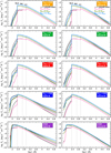 |
Fig. B.2. Same as Fig. 2, but differences between SEDs are shown for smooth (black lines) and clumped (colored lines) wind models for higher (left panels) and reduced (right panels) mass-loss rate Ṁ. |
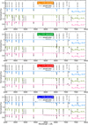 |
Fig. B.7. Same as Fig. 6, but assuming a mass-loss rate hundred times lower than nominal (i.e. higher) value. |
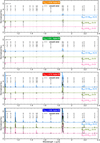 |
Fig. B.10. Same as Fig. 6, but in the IR region. |
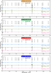 |
Fig. B.11. Same as Fig. B7, but in the IR region. |
All Tables
Mass-loss rate values applied in the synthetic spectra computations, compared to those that Hainich et al. (2015) would predict for the same stars.
All Figures
|
Fig. 1. HR diagram of our models (black symbols) and their corresponding evolutionary sequences. The sequences are taken from Paper I and Szécsi (2016). Initial masses are labeled, showing where the tracks start their evolution, proceeding toward the hot side of the diagram. Colors show the central helium mass fraction, and dots represent every 105 years of evolution. Dashed lines mark equiradial lines with 1, 10, and 100 R⊙ from left to right. The black symbols represent the models for which we computed synthetic spectra. From right to left: black symbols correspond to evolutionary phases with surface helium mass fractions of 0.28, 0.5, 0.75, and 0.98, and the fifth symbol on the very left corresponds to a central helium mass fraction of 0.5, i.e., the middle of the CHeB phase. |
| In the text | |
|
Fig. 2. Spectral energy distribution (continuum) of chemically homogeneously evolving stars in different evolutionary stages as marked in the colored boxes in each panel. Left panels: provide the continuum SED of the models calculated with a smooth (D = 1) wind, while the right panels depict the same for the clumped (D = 10) wind assumption. The colored lines correspond to the models with specific Mini (denoted in the top panels) and calculated assuming the same (nominal) mass-loss rate as given in Table 1. For each colored line, a black line also represents the SED of the model for the same star in the same evolutionary stages with the same clumping factor D, but assuming a mass-loss rate 100 times lower. For better visibility of the differences between the SEDs in the CHeB phase, see Fig. B1. |
| In the text | |
|
Fig. 3. PoWR spectra in the optical region of TWUIN stars with different Mini (see labels on the right sides of the panels) and in different CHB evolutionary phases marked by the value YS in the colored boxes. The colored lines correspond to the models calculated with mass-loss rates as given in Table 1. The black lines correspond to the models of the same stars in the same evolutionary stages, but calculated with mass-loss rates 100 times lower (i.e., reduced Ṁ). In all cases, the spectra correspond to smooth (D = 1) wind models. |
| In the text | |
|
Fig. 4. Top panel: same as Fig. 3, but for the CHeB evolutionary phase with YS as given in Table 1. Middle and lowest panels: same as the top panel, but for clumped wind (i.e., D = 10) with nominal (i.e., higher) Ṁ (middle panel) and reduced Ṁ (lowest panel); black lines correspond to the model with smooth wind assumption. |
| In the text | |
|
Fig. 5. Same as Fig. 3, but zooming in on the He II λ4686 Å line (upper panels) and Hα line blended with He II λ6560 Å line (lower panels). In the CHeB evolutionary phase, the C IV λ4657 Å line appears. |
| In the text | |
|
Fig. 6. PoWR spectra in the optical region of TWUIN stars with different Mini (see labels on the right side of the panels) and in different CHB evolutionary phases marked by the value YS in the colored boxes. The mass-loss rates are taken from the stellar evolutionary calculations (i.e., higher Ṁ). Colored lines correspond to the clumped wind models (i.e., D = 10), while the black lines correspond to the smooth wind. |
| In the text | |
|
Fig. 7. Influence of clumping on the line strength. Emission lines in the optical (upper panels), the UV (middle panels), and the IR (lower panels) regions of the model with Mini = 131 M⊙ in the CHeB evolutionary phase (mass-loss rate of log(Ṁ/M⊙/yr = −4.23)). X-axis is centered around the wavelength indicated by the key legend (e.g., He II 4686 means He II λ4686 Å). Green lines corresponds to clumped wind models with D = 10, and black lines to smooth wind models with D = 1. |
| In the text | |
|
Fig. 8. Comparison of one of our representative O 3 III spectra (i.e., the TWUIN T-8 model, see Table 1) to an O 3 synthetic star from the literature. Both stars are placed at the same distance of 10 pc. An effect of line broadening due to fast rotation is taken into account, as described in Sect. 4 assuming the same rotational velocity, which corresponds to the T-8 model. See Sect. 6.1 for more details. |
| In the text | |
|
Fig. 9. Same as Fig. 8, but comparing our WO 1 spectra (i.e., TWUIN T-10 model, see Table 1) to an SMC WO 4 synthetic spectrum from Shenar et al. (2016). |
| In the text | |
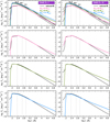 |
Fig. B.1. Same as Fig. 2, but only for CHeB evolutionary phase. |
| In the text | |
|
Fig. B.2. Same as Fig. 2, but differences between SEDs are shown for smooth (black lines) and clumped (colored lines) wind models for higher (left panels) and reduced (right panels) mass-loss rate Ṁ. |
| In the text | |
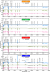 |
Fig. B.3. Same as Fig. 3, but in the UV region. |
| In the text | |
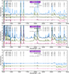 |
Fig. B.4. Same as Fig. 4, but in the UV region. |
| In the text | |
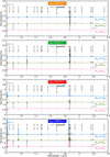 |
Fig. B.5. Same as Fig. 3, but in the IR region. |
| In the text | |
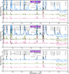 |
Fig. B.6. Same as Fig. 4, but in the IR region. |
| In the text | |
|
Fig. B.7. Same as Fig. 6, but assuming a mass-loss rate hundred times lower than nominal (i.e. higher) value. |
| In the text | |
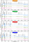 |
Fig. B.8. Same as Fig. 6, but in the UV region. |
| In the text | |
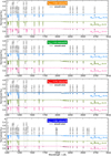 |
Fig. B.9. Same as Fig. B7, but in the UV region. |
| In the text | |
|
Fig. B.10. Same as Fig. 6, but in the IR region. |
| In the text | |
|
Fig. B.11. Same as Fig. B7, but in the IR region. |
| In the text | |
Current usage metrics show cumulative count of Article Views (full-text article views including HTML views, PDF and ePub downloads, according to the available data) and Abstracts Views on Vision4Press platform.
Data correspond to usage on the plateform after 2015. The current usage metrics is available 48-96 hours after online publication and is updated daily on week days.
Initial download of the metrics may take a while.