| Issue |
A&A
Volume 621, January 2019
|
|
|---|---|---|
| Article Number | A140 | |
| Number of page(s) | 11 | |
| Section | Interstellar and circumstellar matter | |
| DOI | https://doi.org/10.1051/0004-6361/201834173 | |
| Published online | 18 January 2019 | |
Extreme fragmentation and complex kinematics at the center of the L1287 cloud
1
Institut de Ciències de l’Espai, CSIC, Campus UAB, Carrer de Can Magrans, s/n 08193 Cerdanyola del Vallès,
Barcelona,
Catalonia,
Spain
2
Institut d’Estudis Espacials de Catalunya (IEEC),
Barcelona,
Catalonia,
Spain
3
Departament de Física Quàntica i Astrofísica, Institut de Ciències del Cosmos (ICCUB)★, Universitat de Barcelona (IEEC-UB),
Martí Franquès 1,
08028
Barcelona,
Catalonia,
Spain
4
European Southern Observatory (ESO),
Karl-Schwarzschild-Str. 2,
85748
Garching,
Germany
e-mail: hyliu@asiaa.sinica.edu.tw
5
Instituto de Radioastronomía y Astrofísica, Universidad Nacional Autónoma de México,
PO Box 3-72,
58090,
Morelia,
Michoacán,
Mexico
6
Institute of Astronomy and Astrophysics, Academia Sinica,
PO Box 23-141,
Taipei 106,
Taiwan
7
National Astronomical Observatories, Chinese Academy of Sciences,
Chaoyang,
PR China
8
Max-Planck-Institut für Radioastronomie,
53121
Bonn,
Germany
Received:
2
September
2018
Accepted:
19
November
2018
Aims. The filamentary ~10-pc-scale infrared dark cloud L1287 located at a parallax distance of ~929 pc is actively forming a dense cluster of low-mass young stellar objects (YSOs) at its inner ~0.1 pc region. To help understand the origin of this low-mass YSO cluster, the present work aims at resolving the gas structures and kinematics with high angular resolution.
Methods. We performed ~1′′ angular resolution (~930 AU) observations at ~1.3 mm wavelengths using the Submillimeter Array (SMA), which simultaneously cover the dust continuum emission and various molecular line tracers for dense gas, warm gas, shocks, and outflows.
Results. From a 1.3-mm continuum image with a resolution of ~2′′ we identified six dense cores, namely SMA1-6. Their gas masses are in the range of ~0.4–4 M⊙. From a 1.3-mm continuum image with a resolution of ~1′′, we find a high fragmentation level, with 14 compact millimeter sources within 0.1 pc: SMA3 contains at least nine internal condensations; SMA5 and SMA6 are also resolved with two internal condensations. Intriguingly, one condensation in SMA3 and another in SMA5 appear associated with the known accretion outburst YSOs RNO 1C and RNO 1B. The dense gas tracer DCN (3–2) well traces the dust continuum emission and shows a clear velocity gradient along the NW-SE direction centered at SMA3. There is another velocity gradient with opposite direction around the most luminous YSO, IRAS 00338 + 6312.
Conclusions. The fragmentation within 0.1 pc in L1287 is very high compared to other regions at the same spatial scales. The incoherent motions of dense gas flows are sometimes interpreted by being influenced by (proto)stellar feedback (e.g., outflows), which is not yet ruled out in this particular target source. On the other hand, the velocities (with respect to the systemic velocity) traced by DCN are small, and the directions of the velocity gradients traced by DCN are approximately perpendicular to those of the dominant CO outflow(s). Therefore, we alternatively hypothesize that the velocity gradients revealed by DCN trace the convergence from the ≳0.1 pc scales infalling motion towards the rotational motions around the more compact (~0.02 pc) sources. This global molecular gas converging flow may feed the formation of the dense low-mass YSO cluster. Finally, we also found that IRAS 00338 + 6312 is the most likely powering source of the dominant CO outflow. A compact blue-shifted outflow from RNO 1C is also identified.
Key words: stars: formation / ISM: individual objects: L1287 / ISM: molecules
© ESO 2019
1 Introduction
Molecular gas filaments collapsing towards the center of molecular clouds may pile up where the centrifugal force is becoming important compared with the gravitational force, and then form dense stellar clusters. The observationally very well resolved examples include the L ~ 107 L⊙ OB cluster-forming region W49A (e.g. Keto et al. 1991; Galván-Madrid et al. 2013; Lin et al. 2016), the L ~ 106 L⊙ OB cluster-forming region G10.6-0.4 (e.g. Keto et al. 1987; Liu et al. 2012a), the L ~ 105 L⊙ OB cluster-forming region G33.92 + 0.11 (e.g. Liu et al. 2012b, 2015), and the L ~ 104 L⊙ OB cluster-forming region NGC6334 V (e.g. Juárez et al. 2017). Is it plausible to form dense clusters of low-mass young stellar objects (YSOs) with a similar mechanism (see Corsaro et al. 2017; Mapelli 2017)?
To try and answer this question, we study the filamentary dark molecular cloud, L1287, which is located at a distance of  pc (Rygl et al. 2010). Its inner, densest ~0.1-pc region is forming a L ~103 L⊙ low-mass YSO cluster (e.g. Estalella et al. 1993; Quanz et al. 2007). Four of the YSOs, namely VLA1-4, are known to be associated with thermal radio jets (Anglada et al. 1994). Based on the previous, lower angular-resolution observations of C18 O (1–0), Umemoto et al. (1999) estimated the enclosed gas mass over the ~ 0.5-pc-scale parent molecular gas structure to be ~120 M⊙. Contrasting to the aforementioned OB cluster-forming regions, the bolometric luminosity of L1287 is not contributed by the nuclear burning of OB stars, but instead is contributed by the accretion luminosity of the low-mass protostars, including two known FU Orionis objects1 RNO 1B/1C(Staude & Neckel 1991; Kenyon et al. 1993; McMuldroch et al. 1995; Quanz et al. 2007), and a L ~ 600 L⊙ Class 0/I YSO IRAS 00338 + 6312 (Anglada et al. 1994). Earlier observations resolved bipolar CO outflow(s) aligning in the NE-SW direction (Snell et al. 1990; Yang et al. 1991; Fehér et al. 2017), although the identification of the powering source(s) remains uncertain.
In this paper, we report the ~ 1′′ (~ 930 AU)-angular-resolution observations with the Submillimeter Array (SMA)2, covering the inner ~0.25-pc region of L1287. By examining the resolved 1.3 mm dust continuum emission and various molecular line tracers of dense gas, warm gas, shocks, and outflows, our aim is to elucidate how the gas flows converge from parsec scales (e.g., due to gravitational collapse) down to ~ 1000 AU scales, and how they are dynamically forming the low-mass YSO cluster. We also provide a more definite identification of the powering source of the previously reported molecular outflows.
The details of our observations are presented in Sect. 2. The observational results from the dust continuum and molecular line emission are given in Sect. 3. In Sect. 4 we present an analysis of fragmentation, dense gas kinematics, and powering sources of the previously reported CO outflows. Our conclusions are given in Sect. 5.
SMA observations summary.
2 Observations and data reduction
2.1 Submillimeter Array observations
We performed five tracks of SMA observations at ~1.3 mm wavelengths towards the inner ~0.25-pc region of L1287 between August 2013 and July 2014, which are summarized in Table 1. The pointing and phase referencing centers of the observationsare RA(J2000) = 00h36m46.65s, Dec(J2000) = + 63°28′57.90″. The projected baselines of these observations range from ~4 to ~ 140 kλ. The system temperature Tsys for all the observations was around 150 K.
The observations were obtained with the 230 GHz receiver, with 4 GHz bandwidth in each of the upper and lower sidebands. The correlator consisted of 48 chunks, each with a bandwidth of 104 MHz. The frequency was centered at 231.3 GHz at chunk 35 of the upper sideband (USB). This configured the correlator with the lower sideband (LSB) covering from 216.48 to 220.46 GHz and the USB from 228.46 to 232.43 GHz. These frequency ranges covered the molecular lines listed in Table A.1. The 13CO and N2 D+ lines were observed with 512 channels per chunk and a spectral resolution of 0.26 km s−1, and the line NH2 D was observed with 256 channels per chunk giving 0.53 km s−1 spectral resolution. The remaining lines were observed with 128 channels per chunk and a 1.06 km s−1 spectral resolution. To generate the 1.3 mm continuum, we averaged the line-free channels in the lower and upper sidebands. The continuum data have been reported by Liu et al. (2018) as part of a SMA survey towards 29 accretion-outburst YSOs. These latter authors did not analyze the details of the extended structures, and did not analyze spectral line data.
The calibration for absolute flux, bandpass, and gain were carried out using the MIR IDL software package3. The images were created using the Multichannel Image Reconstruction, Image Analysis, and Display (MIRIAD, Sault et al. 1995) software package.
To map the rather extended gas flows, we used ROBUST = 1 weighting (Briggs 1995) to create the 1.3-mm dust continuum emission map using all data listed in Table 1, which yielded a 2′′28 × 2′′17 (PA = −19°) synthesized beam, and an rms noise level of 0.6 mJy beam−1. In addition, we created a higher angular-resolution 1.3-mm dust continuum emission map of spatially compact sources using only the observations taken in the extended array configuration. We used a ROBUST = 0 weighting, which yielded a synthesized beam of 0′′96 × 0′′79 (PA = −22°) and an RMS noise level of 0.5 mJy beam−1.
To present the maps of the molecular lines, we applied three different weightings. For most of the lines that show extended emission we used a ROBUST = 2 weighting (i.e., natural weighting), which provides the best sensitivity. For the CO (2–1) line we used a ROBUST = 0 weighting to obtain a better angular resolution. Finally, for OCS (18–17), HNCO 10(0,10)–9(0,9), and CH3 OH 3(− 2,2)–4(− 1,4), which present spatially compact emission, we used only data from the extended and compact array configurations and a ROBUST = 2 weighting.
2.2 Archival Herschel images
To present the structures of the parent molecular cloud on scales of 1–10 pc, and to estimate the dust temperature, we retrieved the Herschel-SPIRE 250, 350, and 500 μm images, which were taken as part of the Herschel infrared Galactic Plane (Hi-GAL) survey (obsID:1342249229, Molinari et al. 2010).
We smoothed the 250 and 350 μm images to the angular resolution of the 500 μm image (37′′), and then derived gas column density (N(H2)) and dust temperature (Td) pixel-by-pixel by fitting the modified-black-body spectrum
 (1)
(1)
where Sν is the flux observed at frequency ν, Ωm is the considered solid angle, Bν(Td) is the Planck function at Td, and τν is the dust optical depth. We converted τν to the gas column density N(H2) by assuming
 (2)
(2)
where R is the gas-to-dust mass ratio which we assumed to be 100, μ = 2.8 is the mean molecular weight, mH is the mass of a hydrogen atom, and κν is the dust mass opacity which is assumed to have the following dependence on frequency ν
![\begin{equation*} \kappa_{\nu} = \kappa_{\mbox{\scriptsize 230 GHz}}\,\Bigg[\frac{\nu \mbox{\,[GHz]}}{230}\Bigg]^{\beta}, \end{equation*}](/articles/aa/full_html/2019/01/aa34173-18/aa34173-18-eq4.png) (3)
(3)
where κ230 = 0.9 cm2 g−1 (Ossenkopf & Henning 1994). We assumed a dust emissivity index β of 1.8. We refer to Hildebrand (1983) for an introduction to the formulation we are based on.
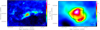 |
Fig. 1 37′′ angular resolution gas column density (N(H2); left panel) and dust temperature (Td; right panel) maps of L1287 (for more details see Sect. 2.2). The black box in both panels indicates the field of view of the top panel of Fig. 2, which presents the 1.3 mm continuum image taken with the SMA. |
3 Results
3.1 Dust continuum
Figure 1 shows the large-scale N(H2) and Td maps of L1287. On 1–10 pc scales this molecular cloud presents a filamentary morphology, with a dense molecular gas hub (see Myers 2009) located at its central ~0.5 pc region. The Td map shows two higher temperature lobes to the NE and SW of the hub, which may be associated with heated cavities created by the bipolar CO outflow(s) emanated from the embedded low-mass YSO cluster (Snell et al. 1990; Yang et al. 1991; Quanz et al. 2007).
Figure 2 shows the SMA 1.3 mm continuum image on the central region of the hub. The continuum emission at 1.3 mm can arise from dust thermal emission and free–free emission. Based on the deep VLA observations of the centimeter free–free continuum emission presented in Anglada et al. (1994), we constrained the 1.3-mm free–free emission to be < 0.5 mJy towards IRAS 0038 + 6312 and RNO 1C. When compared to the detected emission level in Fig. 2, we consider that the contribution of free–free emission is in general negligible.
The 2′′ resolution 1.3-mm dust continuum emission (top panel of Fig. 2) splits up into six main cores (defined with at least a 35σ closed contour), which are spatially separated bya mean distance of ~0.03 pc (~ 6500 au), and have a mean size of ~0.02 pc (~ 4500 au). Assuming that the dust emission is optically thin, we estimated the gas and dust masses of these cores based on the following formulation
 (4)
(4)
where d is the distance. Here we adopted κν = 0.9 cm2 g−1 for thin ice mantles after 105 yr of coagulation at a gas density of 106 cm−3 and for the frequency of our observations (Ossenkopf & Henning 1994). For these estimates we assumed Td = 22 K, which is the averaged dust temperature we derived in this region based on the Herschel data (Fig. 1, right).
The derived masses of these six main cores are in the range of ~ 0.4–4 M⊙. The central core (SMA3; harboring RNO 1C and VLA 1) and the northeastern core (SMA1; harboring IRAS 0038 + 6312 and VLA 3) are the most massive ones, with ~4 and ~ 2 M⊙, respectively. The faintest core, SMA4, which may harbor VLA 4, is located SE of the central core, and has a mass of ~ 0.4 M⊙. The faint and small core (SMA5) located S of the central core seems to be associated with the FU Orionis object RNO 1B and has a mass of ~ 0.6 M⊙. The overall mass recovered by our SMA 1.3-mm continuum image is 22 M⊙.
To better resolve the internal fragmentation in this region, we present the 1.3-mm continuum image generated using only the extended configuration data (i.e., ~1′′ angular resolution; Table 1), which is shown in the bottom panel of Fig. 2. The highest-mass core, SMA3, is resolved into a ~ 0.02 pc scale clumpy toroid containing at least nine internal gas condensations; SMA3b and SMA3c may be associated with the YSO(s) RNO 1C and VLA 1; SMA2 appears to be a ~0.02 pc scale, elongated arm-like structure connecting to the clumpy toroid from the north; SMA5 and SMA6 may be parts of another ~ 0.04-pc-scale, elongated arm-like structure connecting to the clumpy toroid from the south. Overall, we identify 14 condensations with at least a 7σ closed contour. Wemeasured the flux density of each condensation by fitting an elliptical Gaussian using the MIRIAD task IMFIT, and then based on Eq. (4) we estimated the gas and dust masses. The polygons for fitting the Gaussian were drawn following the 6σ and the 9σ contour levels for the most extended sources (1σ = 0.5 mJy beam−1). The derived masses range between ~0.1 and ~ 0.7 M⊙. The properties derived from these fits also included the peak position, the deconvolved angular size and position angle, and the intensity of the peak. The results are listed in Table 2. We note that the total flux obtained taking into account only the extended configuration is ~16% of the total flux obtained with all the configurations combined. This is due to the filtering effect of the extended emission.
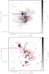 |
Fig. 2 Top panel: 1.3-mm dust continuum emission with extended, compact, and subcompact configurations. Contours are − 6, − 3, 3, 6, 9, 20, 30, 38, 49, 60, 70, 80, and 90 times the rms level of the map, 0.6 mJy beam−1. Black ellipsecorresponds to the position error ellipse for IRAS 00338 + 6312. The synthesized beam located at the bottom right is 2′′28 × 2′′17, PA = − 19°. The gray square corresponds to the field of view of the bottom panel. A scale bar is located in the upper-left corner. Bottom panel: 1.3-mm dust continuum emission with extended configuration. Contours are − 3, 3, 6, 9, 12, 15, 18, 21, 24, 27 and 30 times the rms level of the map, 0.5 mJy beam−1. Sources (labeled in red) are defined as having at least a 7σ closed contour. Red contours are drawn following the 6 and 9 sigma contour levels for themost extended sources. The synthesized beam located at the bottom right is 0′′ 96 × 0′′79, PA = − 22°. A scale bar is shown in the lower left corner. Blue concave hexagons and pink crosses in both panels are radio (Anglada et al. 1994)and infrared (Quanz et al. 2007) sources, respectively. |
3.2 Molecular lines
In addition to the dust continuum emission, a number of molecular lines were detected with the SMA within the 8 GHz bandwidth. We identified 15 molecular lines of CH3OH, SO, OCS, SiO, H2CO, HNCO, DCN, DNC and CO. Table A.1 lists the frequency, the energy of the upper level, and the estimated critical density for each transition. In Fig. 3, we present the velocity integrated emission (i.e., moment 0) maps of several of the detected transitions in L1287.
The shock tracer SiO (5–4) reveals compact emission towards IRAS 00338 + 6312, RNO1C, VLA 4 and the dust continuum core SMA6. Also, it presents compact emission, neither associated with dust continuum emission nor to any YSO, towards the east, west, and southwestern parts of the region. SO 6(5)–5(4) emission traces similar structures with those traced by SiO (5–4), but presents more prominent extended emission covering the central part of the observed region. In addition, the SO 6(5)–5(4) emission is more extended than SiO emission in the southwest, forming a “V” shaped structure. CH3OH 8(− 1,8)–7(0,7), H2 CO 3(0,3)–2(0,2), and 3(2,1)–2(2,0) emission present similar morphology to SiO and SO, but additionally show bright emission towards VLA 2 and are fainter around RNO 1C. DCN (3–2) and H2 CO 3(2,1)–2(2,0) transitions trace well the dust continuum emission. The emission extends over the dust continuum presenting the strongest emission at IRAS 0038 + 6312. In addition, DCN (3–2) shows strong emission towards the toroidal dust structure, with fainter emission coinciding with RNO 1C and the center of the dust continuum toroid. Moreover, unresolved emission of CH3OH 5(1,4)–4(2,2), CH3OH 3(− 2,2)–4(− 1,4), OCS (18–17) and HNCO 10(0,10)–9(0,9) is detected at IRAS 0038 + 6312.
In Fig. 4 we present the intensity-weighted averaged velocity (i.e., moment 1) maps of the lines presented in Fig. 3. A Gaussian fit to the DCN (3–2) spectrum averaged from the entire observed region indicates that the systemic velocity of this system is − 17.4 km s−1. The dense core tracers H2 CO 3(0,3)–2(0,2) and 3(2,1)–2(2,0), SO 6(5)–5(4) and more clearly DCN (3–2) show a NW-SE large-scale (~ 0.1 pc) velocity gradient between − 15 and − 19 km s−1 centered at the dust central core (SMA3) near RNO1C and VLA 1. We note that previous single-dish observations of H13CO+ (1–0) also resolved a velocity gradient in the same direction, but extended to a much larger angular scale (~ 2′, ~ 0.6 pc; see Umemoto et al. 1999). In addition, on a smaller spatial scale and around IRAS 0338 +6312, these molecular lines also reveal a velocity gradient in the reversed direction. These velocity gradients are perpendicular to the previously reported, NE-SW bipolar outflow (Snell et al. 1990; Yang et al. 1991). The velocity gradient around IRAS 0338 + 6312 is also seen in CH3OH 8(− 1,8)–7(0,7). The emission towards the SW of the dust continuum emission seen in H2 CO, SO, and SiO is clearly blue-shifted with a velocity of approximately −24 km s−1.
To study the kinematics in the region in more detail, we present the blue- and red-shifted emission of DCN (3–2) in Fig. 5. The first panel presents the emission at ± 1.2 km s−1 from the systemic velocity. The blue- and red-shifted emission shows two structures forming the large-scale and reversed small-scale velocity gradients. At higher velocities (at ± 2.4 and ± 3.6 km s−1), the small-scale velocity gradient centered on IRAS 00338 + 6312 becomes more compact.
Parameters of the sources detected with the SMA at 1.3 mm dust continuum emission.
Molecular outflow
In Fig. 6, we present the red- and blue-shifted high-velocity emission of the CO (2–1) in different velocity ranges. At these high velocities, the CO (2−1) traces molecular outflows. In agreement with the previous observations by Snell et al. (1990) and Yang et al. (1991), the emission shows an extended NE-SW bipolar molecular outflow centered near IRAS 0038 + 6312 (and VLA 3) and the FU Orionis object RNO 1C. However, IRAS 0038 + 6312 seems to fall closer to the center of the bipolar structure (see first and second panels of Fig. 6). Moreover, the red- and blue-shifted emission in the NE and SW lobes, respectively, present clear cavity features, with the southern side of the blue-shifted lobe coinciding with the emission detected with the dense gas tracer H2 CO and the shock tracers SO and SiO. This strongly suggests that the outflow is dragging dense gas from this region (see Figs. 4 and 7), as already observed in other regions (e.g. HH 2: Girart et al. 2005; Lefloch et al. 2005). In the last two panels, at the highest velocities, the blue-shifted emission appears at the position of RNO1C with an elongated structure in the N-S direction. To analyze only the highest-velocity gas from the CO (2–1) emission, the upper panel of Fig. 8 shows the integrated emission between − 51 and − 47 km s−1. The emission at these velocities is compact and appears only very close to the position of RNO 1C. It is also important to note that the shock tracer SiO (5–4) shows emission towards both IRAS 0038 + 6312 and RNO 1C (see Fig. 3).
4 Discussion
4.1 Fragmentation in L1287
In Sect. 3.1 we presented the continuum emission at 1″ angular resolution for L1287, which reveals 14 compact millimeter sources within a region of 0.1 pc. Given the rms noise of the 1″ image, our mass sensitivity is ~ 0.05 M⊙ (making the same assumptions as in Sect. 3.1). This mass sensitivity and our spatial resolution of 930 AU are well below the Jeans mass (~ 0.6 M⊙) and Jeans length (~6200 AU) for a region of density 106 cm−3 and temperature of 20 K (following Palau et al. 2015), and are fully comparable to those reported by Palau et al. (2014, 2015). Thus, the SMA observations presented here are well suited to study fragmentation in L1287.
Palau et al. (2014, 2015) study the fragmentation level of a sample of 19 intermediate- and high-mass dense cores also within a spatial scale of 0.1 pc, and find fragmentation levels ranging from 1 up to 11 sources. The fragmentation level is defined by Palau et al. (2014, 2015) as the number of compact millimeter sources (with at least one closed contour) above 6 times the rms noise of the image, within a region of 0.1 pc of diameter. Therefore, L1287, with 14 compact millimeter sources within 0.1 pc, presents a very high fragmentation level compared to the regions of this sample.
Palau et al. (2014, 2015) study the relation between the fragmentation level and different properties of the host cores, and find possible trends of fragmentation level increasing with the average density within 0.1 pc (with a correlation coefficient of 0.89) and with the ratio of rotational to gravitational energy (with a correlation coefficient of 0.57), usually referred to as βrot. Here, we therefore study whether the average density within 0.1 pc and/or the rotation motions might explain the high fragmentation level in L1287.
In order to obtain a first approximation of the average density within 0.1 pc, we measured the flux density within an angular diameter of 22″ (corresponding to 0.1 pc) in an image of the dust emission obtained with a single dish, so that we avoid the filtering of large-scale emission produced by interferometers. We chose to use the James Clerk Maxwell Telescope data at 450 μm from Di Francesco et al. (2008) because this provides a main beam of 11″ (and an effective beam of 17.3″), which allows us to slightly resolve the emission within 0.1 pc. We obtained a flux density of 56 Jy within 0.1 pc for L1287. Taking into account an average dust temperature within 0.1 pc of 20 K (from the Herschel data presented in Sect. 2.2), this corresponds to an average density of around 106 cm−3. On the other hand, using the DCN velocity gradient of Fig. 10 (bottom), we estimated βrot for L1287, which is of 0.067. In Fig. 9 we plot the fragmentation level versus average density within 0.1 pc, and also versus βrot for the sample of Palau et al. (2014, 2015), including the new results for L1287 (marked as a red symbol). These plots show that L1287 presents a relatively high density and a high βrot when compared to the entire sample of 19 massive dense cores of Palau et al. (2014, 2015). It therefore seems that both gravity and rotational energy could play an important role in the fragmentation process within L1287.
Considering the compact nature of the millimeter fragments, it seems reasonable to think that these fragments will form stars in the near future or are already associated with low-mass YSOs. Thus, our data seem to indicate that L1287 is forming a dense cluster of deeply embedded low-mass YSOs.
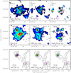 |
Fig. 3 Color scale image of the integrated intensity (i.e., moment 0) maps of selected molecular line tracers overlapped with the contour map of the 1.3 mm dust continuum emission (only using the extended configuration for the dust continuum emission in the middle and lower panels). Pink crosses and black triangles indicate infrared (Quanz et al. 2007) and radio (Anglada et al. 1994) sources, respectively. The synthesized beam of each molecule is located at the bottom-right corner. |
4.2 Dense gas kinematics
For complicated cluster-forming regions resolved with CO outflows, it is always possible to attribute incoherent motions to the influence of outflow feedback or turbulence motions. While with the data presented here we cannot rule out these cases, below we discuss one possibility to coherently interpret the observed dense gas kinematics from large to small spatial scales as gravitational contraction.
An inverse P Cygni line profile (Pirogov et al. 2016), which is consistent with infalling motions on scales of ≳0.1 pc, has been found towards L1287 using single-dish observations of HCO+ and H13CO+ (1–0). On slightly larger scales, of ~0.3–0.5 pc, Umemoto et al. (1999) resolved a blueshifted motion in the NW, and a redshifted motion in the SE. On ~ 0.1-pc scales, our DCN (3–2) and H2CO 3(0,3)-2(0,2) line images (Fig. 4) trace a component of velocity gradient which has approximately the same orientation with the velocity gradient on ~ 0.3–0.5 pc scales. It is therefore natural to consider that our observations of these dense and/or warm gas tracers reveal the innermost part of the coherent gasaccretion flow. Umemoto et al. (1999) interpreted this large-scale velocity gradient as rotational motions, due to the fact that it is perpendicular to the direction of the resolved CO outflow. Alternatively, it remains possible to coherently interpret the large-scale (~ 0.1–0.5 pc) velocity gradient and the inverse P Cygni line profile as infall. The presence of a CO outflow does not require a rotating disk on scales of ≳0.1 pc. The velocities we detect from DCN (3–2) and H2CO 3(0,3)-2(0,2) at ~ 12′′ (0.056 pc) from the center of SMA3 are ~ 2 km s−1. The minimum required mass to gravitationally bind this motion is ~ 25 M⊙, which is consistent with the lower limit of the gas and dust mass we estimated based on the 1.3-mm dust continuum emission (22 M⊙; see Sect. 3.1).
In this context, the reversed velocity gradient on smaller spatial scales around IRAS 00338 + 6312 was unexpected. In Fig. 10, we present the position–velocity (PV) diagrams made at the position angles of 140° and 147°, centered at SMA3 and IRAS 00338 + 6312, respectively. These two velocity gradients clearly have opposite directions. Interestingly, the PV diagram made at the position of IRAS 00338 + 6312 resembles that of a rotating disk, while the other PV diagram does not. From the IRAS 0038 + 6312 velocity gradient, assuming Keplerian motion (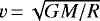 , where v is the velocity, G is the gravitational constant, M is the mass, and R is the radius) and using a radius of 2.5″ and v = 1.25 km s−1, we estimated a mass for IRAS 0038 + 6312 of 4 M⊙. We note that the derived mass here is a lower limit as a possible inclination of the disk is not taken into account. The mass obtained is comparable to the ~ 6 M⊙ obtained by Yang et al. (1991) using the mass-luminosity relation of (L∕L⊙) = (M∕M⊙)4.
If we consider that the small-scale velocity gradient around IRAS 00338 + 6312 is indeed due to rotational motion, then the reversion of the observed velocity gradients may be coherently interpreted as a filamentary large-scale inflow converging towards a circumstellar rotating disk, which may be further associated with the large-scale bipolar CO outflow (Sect. 3.2). The schematic diagram presented in Fig. 11 helps to illustrate this scenario. In the top panel of the figure, we present the blue- and red-shifted integrated DCN map showing the two low-velocity bipolar structures with the reversed velocity gradients. In the bottom panel of the figure, we present our favored interpretation for the reversed velocity gradients. Taking into account the considerations given above, the reversed velocity gradients could be interpreted as converging flows towards the IRAS 00338 + 6312 source. The overall picture of forming a dense YSO cluster in this region from accreting dense gas filaments may therefore be analogous to those OB cluster-forming regions introduced in Sect. 1.
However, we have to point out that, observationally, it has been challenging to robustly distinguish rotational motion from infall, and is harder given the limited spectral resolution of our present observations. While our present interpretation with converging flow is partly motivated by the inverse P Cygni line profile on scales of ≳0.1 pc reported by Pirogov et al. (2016), we cannot yet rule out that our DCN data simply trace independent rotations around two centers, on smaller spatial scales. Future observations of molecular lines with better spectral resolution and higher sensitivity are still required to test our present interpretation.
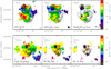 |
Fig. 4 Color scale image of the intensity-weighted average velocity (i.e., moment 1) maps of selected molecular line tracers overlapped with the contour map of the 1.3-mm dust continuum emission. Pink crosses and black triangles indicate infrared (Quanz et al. 2007) and radio (Anglada et al. 1994) sources, respectively. The synthesized beam of each molecule is located at the bottom-right corner. |
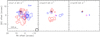 |
Fig. 5 Each panel shows the blue- and red-shifted emission of DCN (3–2) at ± 1.2, ± 2.4, and ± 3.6 kms−1 from the systemic velocity − 17.4 km s−1. Contours are − 4, 4, 8, 12,..., 20, 30, 40, 50 times the rms noise level of the map, 0.03 Jy beam−1. Black and pink crosses are IRAS 0038 + 6312 and RNO1C sources, respectively. The synthesized beam located at the bottom-right corner of the first panel is 1′′ 85 × 1′′77, PA = − 6°. |
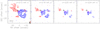 |
Fig. 6 CO (2–1) high-velocity emission. Each panel shows the red- and blue-shifted emission at ± 12, ± 16, ± 20 and ± 24 km s−1 from the systemic velocity − 17.4 km s−1. Contour levels are − 6, 6, 9, ..., 15, 20, 30, 40, ..., 70 and − 3, 3, 6, 9, ..., 15, 20, 30, 40, 50 times the rms level 0.04 Jy beam−1 for the first and the rest of the panels, respectively. Black and pink crosses are IRAS 0038 + 6312 (also VLA 3) and RNO1C sources, respectively. The synthesized beam, located at bottom right of the first panel, is 1′′ 66 × 1′′38, PA = − 8°. A scale bar is located in the bottom-left corner. |
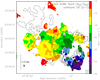 |
Fig. 7 Contours: CO (2–1) red- (dashed) and blue-shifted emission (solid) at ± 12 km s−1 from the systemic velocity − 17.4 km s−1. Contour levels are − 6, 6, 18, 30, 50, 70 times the rms level 0.04 Jy beam−1. The synthesized beam located in the bottom-right corner is 1′′66 × 1′′38, PA = − 8°. Color scale: intensity-weighted averaged velocity (i.e., moment 1) map of H2CO 3(0,3)–2(0,2) emission. A scale bar is located in the bottom-left corner. |
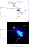 |
Fig. 8 Upperpanel: CO (2–1) highest-velocity emission. Color scale: moment 0 (i.e., integrated intensity) map. Velocity range from − 51 to − 47 km s−1. The synthesized beam located at the bottom right corner is 1′′39 × 1′′27, PA = − 19°. Contours: 1.3-mm dust continuum emission. Pink crosses indicate infrared sources (Quanz et al. 2007). Lower panel: color scale –Hubble Space Telescope image. WFPC2 instrument, F814W filter. |
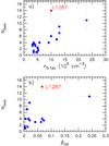 |
Fig. 9 Upper panel: fragmentation level (Nmm) vs. density averaged within a region of 0.1 pc of diameter after Palau et al. (2014, 2015). Bottom panel: fragmentation level vs. rotational-to-gravitational energy after Palau et al. (2014). The location of L1287 in these plots is marked with a red symbol. |
4.3 Powering source of the northeast-southwest molecular outflow
The powering source of the reported northeast-southwest bipolar outflow in L1287 has been a matter of debate in the past, as this is also related to how the accretion and outflows of YSOs are linked (e.g. Evans et al. 1994). Several powering sources have been proposed, including RNO1B/1C (Staude & Neckel 1991) and VLA 3 or IRAS 0038 + 6312 (e.g. Anglada et al. 1994; Yang et al. 1995; Quanz et al. 2007).
By looking at the velocity range within ±20 km s−1 with respectto the systemic velocity (Fig. 6), the facts that IRAS 00338 + 6312 is located closer to the center of the bipolar CO outflow (Sect. 3.2), and that the velocity gradient of the dense gas around it appears perpendicular to the direction of the outflow, indicate that IRAS 00338 + 6312 is a probable powering source and may be associated with a circumstellar (pseudo-)disk. However, at higher velocity (Fig. 6) the bright and blueshifted CO emission appears to be more closely associated with RNO 1C. It may be possible that RNO 1C is also powering a monopolar CO outflow. The spatially compact nature of this outflow could be related to a recent accretion outburst event of this FU Orionis object. Supporting evidence may be the Hubble Space Telescope ~8360 Å (F814W filter) imageshown in the lower panel of Fig. 8. At this wavelength the emission is associated with reflection or scattered light, and we would expect to detect it close to the blueshifted part of the emission, which is indeed the case. The brightest emission is clearly located towards the FU Orionis objects RNO 1B and RNO 1C. The emission also traces well the dust cavity structure seen with the high-angular-resolution image of the SMA with peaks of emission at the SMA3c and SMA3f millimeter sources.
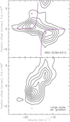 |
Fig. 10 DCN (3–2) position-velocity maps. Upper panel: emission along the velocity gradient at the IRAS 0038 + 6312 source. Contours are − 3, 3, 5, 7, ..., 13 times the rms noise level of the map, 0.03 Jy beam−1. The purple lines indicate a keplerian velocity distribution. Lower panel: emission along the large velocity gradient passing through the center of the toroid traced by the dust continuum emission. Contours are − 3, 3, 6, 9, ..., 24 times the rms noise level of the map, 0.03 Jy beam−1. |
5 Conclusions
We have performed ~ 1′′ angular resolution SMA observations at 230 GHz towards the inner ~ 0.25-pc cluster-forming region of the ~10-pc-scale filamentary dark cloud L1287. Our 1.3-mm dust-continuum image resolves a ~ 0.02-pc-scale clumpy dense gas toroid located at the center, which is surrounded by elongated, 0.02–0.04-pc-scale arm-like dense gas structures and other spatially compact gas overdensities. The fragmentation level found in the region, as compared to previous studies, is very high, with up to 14 compact millimeter sources within a region of 0.1 pc of diameter at a spatial resolution of ~ 1000 AU.
In addition, our observations of the dense molecular gas tracers DCN (3–2) and H2 CO 3(0,3)–2(0,2) resolved two components of velocity gradients: one has approximately the same direction as the velocity gradient traced by previous H13CO+ observations on 0.3–0.5 pc scales; the other is seen on smaller spatial scales around the embedded YSO IRAS 00338 + 6312, and presents a reversed direction. We cannot yet rule out that such incoherent motions are due to the influence of outflow feedback, or due to turbulent motions; and cannot yet rule out that we are seeing independent rotational motions around two centers. However, we find that these motions might be coherently interpreted as a filamentary, 0.1–0.5-pc-scale infalling gas flow, which is converging towards the rotating circumstellar disks on smaller spatial scales. The formation of the low-mass YSO cluster at the center of L1287 might be fed by the global gas inflow, which is analogous to some luminous OB cluster-forming regions such as W49A, G10.6-0.4, G33.92 + 0.11, and NGC6334 V.
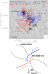 |
Fig. 11 Upper panel: contours correspond to the averaged emission from blue- and red-shifted channels of DCN (3–2) displaying the two low-velocity flow components. Contours are 6, 9, 12, 15, ..., 30 times the rms noise level of the map, 0.03 Jy beam−1. The synthesized beam is located at the bottom right corner. The grey scale corresponds to the 1.3 mm dust continuum emission. The arrows indicate the two possible converging flows of the region. Black crosses indicate the position of infrared sources IRAS 00338 + 6312 and FU-Orionis RNO1B and RNO1C (Quanz et al. 2007). Lower panel: schematic model of the L1287 region. Converging flows + rotation dynamics. The blue and red lines indicate the ~ 0.1 pc scale molecular gas converging towards the center. We can observe a reversed velocity gradient projected towards our line of sight as we can see at the IRAS 00338 + 6312 source. |
Acknowledgements
We thank the SMA staff for their support which makes these studies possible. C.J. acknowledges support from MINECO (Spain) BES-2012-052481 grant. C.J., J.M.G. and G.B. acknowledge support from MICINN (Spain) AYA2014-57369-C3 and AYA2017-84390-C2-2-R grants. A.P. acknowledges financial support from UNAM and CONACyT, México. R.G.M. acknowledges support from UNAM-PAPIIT program IA102817.
Appendix A Line identifications
In this appendix we present a table with the list of detected transitions towards L1287 with the SMA (Table A.1).
Molecular lines detected with the SMA towards L1287.
References
- Anglada, G., Rodriguez, L. F., Girart, J. M., Estalella, R., & Torrelles, J. M. 1994, ApJ, 420, L91 [NASA ADS] [CrossRef] [Google Scholar]
- Beltrán, M. T., Estalella, R., Anglada, G., Rodríguez, L. F., & Torrelles, J. M. 2001, AJ, 121, 1556 [NASA ADS] [CrossRef] [Google Scholar]
- Briggs, D. S. 1995, BAAS, 27, 1444 [Google Scholar]
- Corsaro, E., Lee, Y.-N., García, R. A., et al. 2017, Nat. Astron., 1, 0064 [NASA ADS] [CrossRef] [Google Scholar]
- Di Francesco, J., Johnstone, D., Kirk, H., MacKenzie, T., & Ledwosinska, E. 2008, ApJS, 175, 277 [NASA ADS] [CrossRef] [Google Scholar]
- Estalella, R., Mauersberger, R., Torrelles, J. M., et al. 1993, ApJ, 419, 698 [NASA ADS] [CrossRef] [Google Scholar]
- Evans, II, N. J., Balkum, S., Levreault, R. M., Hartmann, L., & Kenyon, S. 1994, ApJ, 424, 793 [NASA ADS] [CrossRef] [Google Scholar]
- Fehér, O., Kóspál, Á., Ábrahám, P., Hogerheijde, M. R., & Brinch, C. 2017, A&A, 607, A39 [NASA ADS] [CrossRef] [EDP Sciences] [Google Scholar]
- Galván-Madrid, R., Liu, H. B., Zhang, Z.-Y., et al. 2013, ApJ, 779, 121 [NASA ADS] [CrossRef] [Google Scholar]
- Girart, J. M., Viti, S., Estalella, R., & Williams, D. A. 2005, A&A, 439, 601 [NASA ADS] [CrossRef] [EDP Sciences] [Google Scholar]
- Hartmann, L., & Kenyon, S. J. 1985, ApJ, 299, 462 [NASA ADS] [CrossRef] [Google Scholar]
- Herbig, G. H. 1977, ApJ, 217, 693 [NASA ADS] [CrossRef] [Google Scholar]
- Hildebrand, R. H. 1983, QJRAS, 24, 267 [NASA ADS] [Google Scholar]
- Ho, P. T. P., Moran, J. M., & Lo, K. Y. 2004, ApJ, 616, L1 [NASA ADS] [CrossRef] [Google Scholar]
- Juárez, C., Girart, J. M., Zamora-Avilés, M., et al. 2017, ApJ, 844, 44 [NASA ADS] [CrossRef] [Google Scholar]
- Kenyon, S. J., Hartmann, L., Gomez, M., Carr, J. S., & Tokunaga, A. 1993, AJ, 105, 1505 [NASA ADS] [CrossRef] [Google Scholar]
- Keto, E. R., Ho, P. T. P., & Haschick, A. D. 1987, ApJ, 318, 712 [NASA ADS] [CrossRef] [Google Scholar]
- Keto, E. R., Lattanzio, J. C., & Monaghan, J. J. 1991, ApJ, 383, 639 [NASA ADS] [CrossRef] [Google Scholar]
- Lefloch, B., Cernicharo, J., Cabrit, S., & Cesarsky, D. 2005, A&A, 433, 217 [NASA ADS] [CrossRef] [EDP Sciences] [Google Scholar]
- Lin, Y., Liu, H. B., Li, D., et al. 2016, ApJ, 828, 32 [NASA ADS] [CrossRef] [Google Scholar]
- Liu, H. B., Quintana-Lacaci, G., Wang, K., et al. 2012a, ApJ, 745, 61 [NASA ADS] [CrossRef] [Google Scholar]
- Liu, H. B., Jiménez-Serra, I., Ho, P. T. P., et al. 2012b, ApJ, 756, 10 [NASA ADS] [CrossRef] [Google Scholar]
- Liu, H. B., Galván-Madrid, R., Jiménez-Serra, I., et al. 2015, ApJ, 804, 37 [NASA ADS] [CrossRef] [Google Scholar]
- Liu, H. B., Dunham, M. M., Pascucci, I., et al. 2018, A&A, 612, A54 [NASA ADS] [CrossRef] [EDP Sciences] [Google Scholar]
- Mapelli, M. 2017, MNRAS, 467, 3255 [NASA ADS] [CrossRef] [Google Scholar]
- McMuldroch, S., Blake, G. A., & Sargent, A. I. 1995, AJ, 110, 354 [NASA ADS] [CrossRef] [Google Scholar]
- Molinari, S., Swinyard, B., Bally, J., et al. 2010, A&A, 518, L100 [NASA ADS] [CrossRef] [EDP Sciences] [Google Scholar]
- Myers, P. C. 2009, ApJ, 700, 1609 [NASA ADS] [CrossRef] [EDP Sciences] [Google Scholar]
- Ossenkopf, V., & Henning, T. 1994, A&A, 291, 943 [NASA ADS] [Google Scholar]
- Palau, A., Fuente, A., Girart, J. M., et al. 2013, ApJ, 762, 120 [NASA ADS] [CrossRef] [Google Scholar]
- Palau, A., Estalella, R., Girart, J. M., et al. 2014, ApJ, 785, 42 [NASA ADS] [CrossRef] [Google Scholar]
- Palau, A., Ballesteros-Paredes, J., Vázquez-Semadeni, E., et al. 2015, MNRAS, 453, 3785 [NASA ADS] [CrossRef] [Google Scholar]
- Pirogov, L. E., Shul’ga, V. M., Zinchenko, I. I., et al. 2016, Astron. Rep., 60, 904 [NASA ADS] [CrossRef] [Google Scholar]
- Quanz, S. P., Henning, T., Bouwman, J., Linz, H., & Lahuis, F. 2007, ApJ, 658, 487 [NASA ADS] [CrossRef] [Google Scholar]
- Rygl, K. L. J., Brunthaler, A., Reid, M. J., et al. 2010, A&A, 511, A2 [NASA ADS] [CrossRef] [EDP Sciences] [Google Scholar]
- Sault, R. J., Teuben, P. J., & Wright, M. C. H. 1995, in Astronomical Data Analysis Software and Systems IV, eds. R. A. Shaw, H. E. Payne, & J. J. E. Hayes, ASP Conf. Ser., 77, 433 [NASA ADS] [Google Scholar]
- Snell, R. L., Dickman, R. L., & Huang, Y.-L. 1990, ApJ, 352, 139 [NASA ADS] [CrossRef] [Google Scholar]
- Staude, H. J., & Neckel, T. 1991, A&A, 244, L13 [NASA ADS] [Google Scholar]
- Umemoto, T., Saito, M., Yang, J., & Hirano, N. 1999, in Star Formation 1999, ed. T. Nakamoto (Japan: Nobeyama Radio Observatory), 227 [Google Scholar]
- Yang, J., Umemoto, T., Iwata, T., & Fukui, Y. 1991, ApJ, 373, 137 [NASA ADS] [CrossRef] [Google Scholar]
- Yang, J., Ohashi, N., & Fukui, Y. 1995, ApJ, 455, 175 [NASA ADS] [CrossRef] [Google Scholar]
FU Orionis objects are young, pre-main sequence stars which are observed to increase their brightness by 4–6 mag in the optical and remain bright for decades (Herbig 1977). The large-amplitude flares are attributed to enhanced accretion from the surrounding circumstellar disk (Hartmann & Kenyon 1985).
The Submillimeter Array is a joint project between the Smithsonian Astrophysical Observatory and the Academia Sinica Institute of Astronomy and Astrophysics, and is funded by the Smithsonian Institution and the Academia Sinica (Ho et al. 2004).
All Tables
Parameters of the sources detected with the SMA at 1.3 mm dust continuum emission.
All Figures
|
Fig. 1 37′′ angular resolution gas column density (N(H2); left panel) and dust temperature (Td; right panel) maps of L1287 (for more details see Sect. 2.2). The black box in both panels indicates the field of view of the top panel of Fig. 2, which presents the 1.3 mm continuum image taken with the SMA. |
| In the text | |
|
Fig. 2 Top panel: 1.3-mm dust continuum emission with extended, compact, and subcompact configurations. Contours are − 6, − 3, 3, 6, 9, 20, 30, 38, 49, 60, 70, 80, and 90 times the rms level of the map, 0.6 mJy beam−1. Black ellipsecorresponds to the position error ellipse for IRAS 00338 + 6312. The synthesized beam located at the bottom right is 2′′28 × 2′′17, PA = − 19°. The gray square corresponds to the field of view of the bottom panel. A scale bar is located in the upper-left corner. Bottom panel: 1.3-mm dust continuum emission with extended configuration. Contours are − 3, 3, 6, 9, 12, 15, 18, 21, 24, 27 and 30 times the rms level of the map, 0.5 mJy beam−1. Sources (labeled in red) are defined as having at least a 7σ closed contour. Red contours are drawn following the 6 and 9 sigma contour levels for themost extended sources. The synthesized beam located at the bottom right is 0′′ 96 × 0′′79, PA = − 22°. A scale bar is shown in the lower left corner. Blue concave hexagons and pink crosses in both panels are radio (Anglada et al. 1994)and infrared (Quanz et al. 2007) sources, respectively. |
| In the text | |
|
Fig. 3 Color scale image of the integrated intensity (i.e., moment 0) maps of selected molecular line tracers overlapped with the contour map of the 1.3 mm dust continuum emission (only using the extended configuration for the dust continuum emission in the middle and lower panels). Pink crosses and black triangles indicate infrared (Quanz et al. 2007) and radio (Anglada et al. 1994) sources, respectively. The synthesized beam of each molecule is located at the bottom-right corner. |
| In the text | |
|
Fig. 4 Color scale image of the intensity-weighted average velocity (i.e., moment 1) maps of selected molecular line tracers overlapped with the contour map of the 1.3-mm dust continuum emission. Pink crosses and black triangles indicate infrared (Quanz et al. 2007) and radio (Anglada et al. 1994) sources, respectively. The synthesized beam of each molecule is located at the bottom-right corner. |
| In the text | |
|
Fig. 5 Each panel shows the blue- and red-shifted emission of DCN (3–2) at ± 1.2, ± 2.4, and ± 3.6 kms−1 from the systemic velocity − 17.4 km s−1. Contours are − 4, 4, 8, 12,..., 20, 30, 40, 50 times the rms noise level of the map, 0.03 Jy beam−1. Black and pink crosses are IRAS 0038 + 6312 and RNO1C sources, respectively. The synthesized beam located at the bottom-right corner of the first panel is 1′′ 85 × 1′′77, PA = − 6°. |
| In the text | |
|
Fig. 6 CO (2–1) high-velocity emission. Each panel shows the red- and blue-shifted emission at ± 12, ± 16, ± 20 and ± 24 km s−1 from the systemic velocity − 17.4 km s−1. Contour levels are − 6, 6, 9, ..., 15, 20, 30, 40, ..., 70 and − 3, 3, 6, 9, ..., 15, 20, 30, 40, 50 times the rms level 0.04 Jy beam−1 for the first and the rest of the panels, respectively. Black and pink crosses are IRAS 0038 + 6312 (also VLA 3) and RNO1C sources, respectively. The synthesized beam, located at bottom right of the first panel, is 1′′ 66 × 1′′38, PA = − 8°. A scale bar is located in the bottom-left corner. |
| In the text | |
|
Fig. 7 Contours: CO (2–1) red- (dashed) and blue-shifted emission (solid) at ± 12 km s−1 from the systemic velocity − 17.4 km s−1. Contour levels are − 6, 6, 18, 30, 50, 70 times the rms level 0.04 Jy beam−1. The synthesized beam located in the bottom-right corner is 1′′66 × 1′′38, PA = − 8°. Color scale: intensity-weighted averaged velocity (i.e., moment 1) map of H2CO 3(0,3)–2(0,2) emission. A scale bar is located in the bottom-left corner. |
| In the text | |
|
Fig. 8 Upperpanel: CO (2–1) highest-velocity emission. Color scale: moment 0 (i.e., integrated intensity) map. Velocity range from − 51 to − 47 km s−1. The synthesized beam located at the bottom right corner is 1′′39 × 1′′27, PA = − 19°. Contours: 1.3-mm dust continuum emission. Pink crosses indicate infrared sources (Quanz et al. 2007). Lower panel: color scale –Hubble Space Telescope image. WFPC2 instrument, F814W filter. |
| In the text | |
|
Fig. 9 Upper panel: fragmentation level (Nmm) vs. density averaged within a region of 0.1 pc of diameter after Palau et al. (2014, 2015). Bottom panel: fragmentation level vs. rotational-to-gravitational energy after Palau et al. (2014). The location of L1287 in these plots is marked with a red symbol. |
| In the text | |
|
Fig. 10 DCN (3–2) position-velocity maps. Upper panel: emission along the velocity gradient at the IRAS 0038 + 6312 source. Contours are − 3, 3, 5, 7, ..., 13 times the rms noise level of the map, 0.03 Jy beam−1. The purple lines indicate a keplerian velocity distribution. Lower panel: emission along the large velocity gradient passing through the center of the toroid traced by the dust continuum emission. Contours are − 3, 3, 6, 9, ..., 24 times the rms noise level of the map, 0.03 Jy beam−1. |
| In the text | |
|
Fig. 11 Upper panel: contours correspond to the averaged emission from blue- and red-shifted channels of DCN (3–2) displaying the two low-velocity flow components. Contours are 6, 9, 12, 15, ..., 30 times the rms noise level of the map, 0.03 Jy beam−1. The synthesized beam is located at the bottom right corner. The grey scale corresponds to the 1.3 mm dust continuum emission. The arrows indicate the two possible converging flows of the region. Black crosses indicate the position of infrared sources IRAS 00338 + 6312 and FU-Orionis RNO1B and RNO1C (Quanz et al. 2007). Lower panel: schematic model of the L1287 region. Converging flows + rotation dynamics. The blue and red lines indicate the ~ 0.1 pc scale molecular gas converging towards the center. We can observe a reversed velocity gradient projected towards our line of sight as we can see at the IRAS 00338 + 6312 source. |
| In the text | |
Current usage metrics show cumulative count of Article Views (full-text article views including HTML views, PDF and ePub downloads, according to the available data) and Abstracts Views on Vision4Press platform.
Data correspond to usage on the plateform after 2015. The current usage metrics is available 48-96 hours after online publication and is updated daily on week days.
Initial download of the metrics may take a while.