| Issue |
A&A
Volume 621, January 2019
|
|
|---|---|---|
| Article Number | A9 | |
| Number of page(s) | 15 | |
| Section | Cosmology (including clusters of galaxies) | |
| DOI | https://doi.org/10.1051/0004-6361/201730931 | |
| Published online | 19 December 2018 | |
Nitrogen abundance in the X-ray halos of clusters and groups of galaxies
1 SRON Netherlands Institute for Space Research, Sorbonnelaan 2, 3584 CA Utrecht, The Netherlands
e-mail: This email address is being protected from spambots. You need JavaScript enabled to view it.
2 Leiden Observatory, Leiden University, Niels Bohrweg 2, 2300 RA Leiden, The Netherlands
3 Institute of Astronomy, Madingley Road, CB3 0HA Cambridge, UK
4 Key Laboratory of Optical Astronomy, National Astronomical Observatories, Chinese Academy of Sciences, 20A Datun Road, Chaoyang District, 100012 Beijing, PR China
5 Argelander-Institut für Astronomie, Universität Bonn, Auf dem Hügel 71, 53121 Bonn, Germany
Received:
4
April
2017
Accepted:
12
September
2018
Abstract
Context. Chemical abundances in the X-ray halos (also known as the intracluster medium, ICM) of clusters and groups of galaxies can be measured via prominent emission line features in their X-ray spectra. Elemental abundances are footprints of time-integrated yields of various stellar populations that have left their specific abundance patterns prior to and during the cluster and group evolution. Aim. We aim to constrain nitrogen abundances in the CHEmical Evolution RGS Sample (CHEERS), which contains 44 nearby groups and clusters of galaxies, to gain a better understanding of their chemical enrichment.
Method. We examined the high-resolution spectra of the CHEERS sample and took various systematic effects in the spectral modelling into account. We compared the observed abundance ratios with those in the Galactic stellar populations and also with predictions from stellar yields (low- and intermediate-mass stars, massive stars, and degenerate stars).
Results. The nitrogen abundance can only be well constrained (≳3σ) in one cluster of galaxies and seven groups of galaxies. The [O/Fe] – [Fe/H] relation of the ICM is comparable to that for the Galaxy, while the [N/Fe] and [N/O] ratios of the ICM are both higher than in the Galaxy. Future studies on nitrogen radial distributions are required to tell whether the obtained higher [N/Fe] and [N/O] ratios are biased as a result of the small extraction region (r/r500 ≲ 0.05) that we adopt here. Since abundances of odd-Z elements are more sensitive to the initial metallicity of stellar populations, accurate abundance measurements of N, Na, and Al are required to better constrain the chemical enrichment in the X-ray halos of clusters and groups of galaxies.
Key words: galaxies: clusters: intracluster medium / X-rays: galaxies: clusters / X-rays: galaxies / techniques: spectroscopic
© ESO 2018
1. Introduction
Clusters of galaxies aggregate baryons and dark matter within large-scale structures that have collapsed under their own gravity. A large portion (∼15 − 20%) of the total mass of a cluster is in the hot (T ∼ 107 − 8 K) X-ray halos (also known as the intracluster medium, ICM), while the member galaxies only make up ∼3 − 5% of the total mass. The rest is in the form of dark matter. The ICM is an attractive laboratory for the study of nucleosynthesis and chemical enrichment (for a review, see Werner et al. 2008). Because of its deep gravitational potential well, a massive cluster (M ≳ 1013 M⊙, Renzini & Andreon 2014) can be considered a “closed-box” (e.g. White et al. 1993), that is, all the metals synthesised by different stellar populations in the member galaxies are conserved within the cluster. This assumption is based on the consistency (Landry et al. 2013) between the total cluster baryon fraction within a certain radius, for instance, r5001, and the cosmic baryon fraction. This assumption does not necessarily hold for less massive groups of galaxies because the gravitational potential well is relatively shallow. When the metals are released through stellar winds, supernovae, etc., various metal transportation mechanisms working in different locations and on different timescales distribute the metals in the X-ray halos. Relevant metal transportation mechanisms include Galactic winds, ram–pressure stripping, AGN–ICM interaction, and galaxy–galaxy interaction (for a review, see Schindler & Diaferio 2008).
Assuming that stellar populations where the metals are synthesised are representative, given stellar yields and observed abundance patterns in the X-ray halos, we are able to place constraints on the chemical enrichment to the largest gravitationally bound systems in the Universe (for a review, see Böhringer & Werner 2010). Given that α elements (e.g. O, Ne, and Mg) are mainly produced in massive stars in core-collapse supernovae (SNcc), and Fe-peak elements are mainly produced in degenerate stars in Type Ia supernovae (SNIa), the SNIa fraction with respect to the total number of supernovae (SNcc plus SNIa) that enriched the ICM can be obtained by either fitting (e.g. Werner et al. 2006b; de Plaa et al. 2006; Sanders & Fabian 2006; Sato et al. 2007; Komiyama et al. 2009) the best-fit elemental abundances with supernova yields, or by directly applying supernova yields to immediately predict the X-ray spectrum (Bulbul et al. 2012). The latter assumes that the ICM can be described as a single-temperature plasma in collisionally ionised equilibrium (CIE). Unlike elements heavier than oxygen, carbon and nitrogen are mainly produced in low- and intermediate-mass stars (for a review, see Nomoto et al. 2013). Thus, the ICM abundances of C and N also provide important information to better understand the chemical enrichment.
Observationally, the abundances of α elements and Fe-peak elements can be measured with both low- and high-resolution grating spectra (e.g. Mernier et al. 2016a; de Plaa et al. 2017; Hitomi Collaboration 2017). Carbon and nitrogen abundances can only be determined from high-resolution grating spectra, such as those obtained with XMM-Newton reflection grating spectrometer (RGS). Xu et al. (2002) first reported the nitrogen abundance in the hot X-ray halo of NGC 4636. Later, the nitrogen abundance was reported in other individual targets (Tamura et al. 2003; Werner et al. 2006a, 2009; Sanders et al. 2008, 2010; Grange et al. 2011) and in the stacked spectra of 62 groups and clusters of galaxies (Sanders & Fabian 2011).
In this work, we systematically study the nitrogen abundance in the CHEmical Evolution RGS Sample (CHEERS; de Plaa et al. 2017), which contains 44 nearby (z < 0.1) X-ray bright cool-core groups and clusters of galaxies. The key sample selection criterion (de Plaa et al. 2017) of the CHEERS sample is that the O VIII Lyα line at ∼ 18.97 Å (rest frame) is detectable (≳5σ) with the RGS.
Throughout the paper we use H0 = 70 km s−1 Mpc−1, ΩM = 0.3, and ΩΛ = 0.7. For the spectral analysis (Sect. 3), we use C-statistics following Kaastra (2017). Unless specified otherwise, all errors correspond to the 68% confidence level for one interesting parameter.
2. Data reduction
We reduced both RGS and EPIC/MOS data following the same procedures as described in Pinto et al. (2015), using the XMM-Newton Science Analysis System2 (SAS) v15.0.0. MOS data are reduced because the reflection grating assemblies (RGAs) are aligned with the light path of the MOS cameras. We used MOS data for screening soft-proton flares and deriving the spatial extent of the source along the dispersion direction of the RGS.
For each observation, we extracted RGS spectra in a ∼3.4 arcmin wide (along the cross-dispersion direction) region centred on the emission peak. This was done by setting the xpsfincl mask to include 99% of the line spread function (LSF) inside the spatial source extraction mask. The extraction region is somewhat different from the circular aperture used for the EPIC data analysis, especially when there is a gradient in temperature structure and/or metal abundances. The spectra and response matrices were converted into SPEX (Kaastra et al. 1996) format through the SPEX task trafo. The RGS modelled background spectra were subtracted.
The spatial extent along the dispersion direction of the source dominates the broadening of the emission lines, which can be described as (Tamura et al. 2004)
 (1)
(1)
where m is the spectral order, Δθ is the offset angle of the source. The average spatial extent of the ICM that includes half of the maximum line flux is ∼2′′, that is to say, the average full width at half maximum (FWHM) of the line profile (Eq. (1)) is ∼0.276 Å (first order) and ∼0.138 Å (second order). The bin size that we used in our data processing with rgsproc is 0.01 Å (first order) and 0.005 Å (second order). Hence we re-binned the RGS spectra by a factor of 10 for both first-order (7−28 Å) and second-order data (7−14 Å), which approximately yielded the optimal binning (1/2−1/3 FWHM, Kaastra & Bleeker 2016) for RGS spectra of the ICM.
3. Spectral analysis
The high-resolution X-ray spectral analysis package SPEX (v3.03) was used to fit the RGS spectra. For CIE plasma modelling, a large portion of the out-dated atomic data from the old version of SPEX (v.2.05) was replaced with more recent results published in the last decade, such as level-resolved radiative recombination data (Badnell 2006; Mao & Kaastra 2016) and an ionisation balance that includes inner-shell ionisation data (Urdampilleta et al. 2017). In addition, atomic data including collisional excitation/de-excitation rates, radiative transition probabilities, and auto-ionisation rates were consistently calculated using the FAC3 code (Gu 2008) and are included in the latest version of SPEX code as well. The Hitomi Soft X-ray Spectrometer (SXS) spectrum of the Perseus cluster offers an unprecedented benchmark of popular atomic codes; we refer to Hitomi Collaboration (2018) for more details.
For each cluster or group of galaxies, we simultaneously fit RGS1 and RGS2 spectra of each observation. Unless specified otherwise, the redshifts and Galactic absorption column densities were frozen to the values given in Pinto et al. (2015). We used the collisional ionisation equilibrium absorption model (de Plaa et al. 2004; Steenbrugge et al. 2005) with a fixed temperature T = 0.5 eV to account for the Galactic neutral absorption. When modelling the thermal component(s) of the ICM, we considered three different differential emission measure (DEM) distributions.
-
The simplest scenario was to assume that the ICM is isothermal so that it can be described as a single-temperature CIE model (denoted as 1T).
-
A more complicated scenario was to assume that the ICM consists of a hotter and a cooler CIE component (denoted as 2T). Abundances of the two thermal components were assumed to be the same, while emission measures and temperatures were let free to vary.
-
The most sophisticated scenario required a multi-temperature DEM distribution. We adopted the GDEM model (de Plaa et al. 2006) here, which assumed a Gaussian distribution of the DEM in log T,
 (2) where x = log(T) and x0 = log(T0), with T and T0 (peak temperature of the distribution) in units of keV, and Y0 is the emission measure. Apparently, when σ = 0, GDEM is identical to 1T. Again, abundances of the multi-temperature components were assumed to be the same.
These three DEM distributions were driven based on the results of Frank et al. (2013), where the authors measured DEM = dY/dT (where Y = ∫nenHdV is the emission measure) distribution of 62 galaxy clusters in the HIFUGCS sample (Zhang et al. 2011). We compared the goodness of fit, based on which, one of the DEM distributions was favoured and reported for each cluster or group. Regardless of the choice of the DEM distribution, the abundances of N, O, Ne, Mg, Fe, and Ni were let free to vary, while the other elements heavier than He were frozen to 0.3 solar (e.g. Fujita et al. 2008; Werner et al. 2013). All the abundances were normalised to the proto-solar abundances of Lodders et al. (2009), that is, zi, ICM/zi, ⊙. The ionisation balance described in Urdampilleta et al. (2017) was used. The spatial broadening was taken into account by convolving the thermal plasma model (1T/2T/GDEM) with the spatial broadening model (lpro).
This general strategy does not necessarily provide an accurate measurement of elemental abundances. Special treatments are required in some cases. When NH I ≳ 7 × 1024 m−2, the Galactic hydrogen column density (denoted as NH) was allowed to vary (de Plaa et al. 2017). When the ICM thermal emission was contaminated by non-thermal emission, a power law component was added accordingly, with parameters fixed to literature values (e.g. for M 87 see Werner et al. 2006a). The derived abundance of a given element is proportional to the equivalent width, that is, the ratio between the line flux and the continuum flux, given that the abundance is determined mainly from a well-resolved emission line. That is to say, any uncertainty in the continuum would also affect the abundance measurement. When the RGS spectra were fitted for a broad wavelength range (7–28 Å in our case), the continuum flux may be slightly over- or under-estimated because of the uncertainties in the calibration of the RGS effective area, background subtraction, etc. Consequently, abundance measurement might be significantly biased compared to the statistical uncertainties in the spectral fit. The top left panel of Fig. 1 shows that the global fit overestimates the nitrogen abundance in M 87. A similar issue was pointed out by Mernier et al. (2015) for their EPIC spectral analysis, and the authors performed a local fit around a specific line of interest to improve the accuracy of the abundance measurement. Here we also performed the local fit (± 1 Å around the line centre) to determine whether the global continuum level was correct. When it was incorrect, the local fit results were adopted. For instance, while the global fit overestimates the N/Fe ratio (2.9 ± 0.3) for M 87, the local fit yields a more accurate N/Fe ratio (1.8 ± 0.2). Other systematic uncertainties regarding the spatial broadening of the line (Appendix B.2) and RGS background model (Appendix B.3) can be found in the Appendix B.
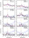 |
Fig. 1. Observed RGS spectra in the N VII neighbourhood, i.e., 23–28 Å wavelength range. The data points are shown in black (RGS1) and grey (RGS2), the modelled background spectra are shown in deep blue (RGS1) and light blue (RGS2) histograms, and the (global fit) model spectra are shown in red (RGS1) and magenta (RGS2) histograms. Vertical dashed lines indicate the O VIII Lyα around 19 Å and N VII Lyα around 25 Å in the observed frame. Spectra from merely one observation per target are shown for clarity. In the global fit to M 87 (top left panel), the N abundance is clearly overestimated, thus a local fit is performed (Sect. 3) to obtain a more accurate abundance measurement. |
4. Results and comparison with literature values
Nitrogen abundance measurements are best made in plasma with lower temperature (Fig. B.1). Therefore, in the CHEERS sample, we found that the nitrogen abundance can merely be well constrained (≳3σ) in the core (r/r500 ≲ 0.05) of one cluster of galaxies (A 3526) and seven groups of galaxies (M 49, M 87, NGC 4636, NGC 4649, NGC 5044, NGC 5813, and NGC 5846). For some sources with lower temperatures (e.g., NGC 3411) in the CHEERS sample, more exposure time is required to better constrain the nitrogen abundance. Spectral fits near the N VII Lyα line for these eight targets are shown in Fig. 1, and the same (global) fits to the 7 − 28 Å wavelength range can be found in Fig. A.1. The abundances and abundance ratios are summarised in Table 1.
Abundances and abundance ratios within the 3.4 arcmin wide (in the cross-dispersion direction) extraction region.
We note that M 87 and A 3526 have the lowest ratio of C-statistics over degrees of freedom (d.o.f., Table 1), but the poor statistics do not significantly affect our astrophysical interpretation of the measured abundance ratios. For instance, there are some features around 27 − 28 Å for M 87, and the two RGS instruments do not agree with each other. Since the source is bright and has a deep exposure, these features are all statistically significant and therefore contribute to the low ratio of the C-statistisc over d.o.f. These features are mainly caused by the imperfect instrument calibration on the effective area. Nevertheless, as shown in Fig. A.1, the global fit yields a good estimate of the continuum and the astrophysical features of the spectrum. Furthermore, we used the local fit to correct biased abundance measurements in the global fit.
The O/Fe ratios in the eight sources (with the extraction region of ∼3.4 arcmin) are ≲1.3. Some of our results differ from those reported in de Plaa et al. (2017) for the 0.8 arcmin wide extraction region. This is mainly due to the strong temperature and abundance gradients (Mernier et al. 2017), if present.
The N/Fe ratios reported in Table 1 are ≳1.4 with larger scatter. Xu et al. (2002), Werner et al. (2006a, 2009), and Grange et al. (2011) also reported similar N/Fe ratio ≳1.4 with large scatter between individual targets. Tamura et al. (2003) reported a lower N/Fe ratio of ∼(0.6 ± 0.2) for NGC 5044. The N/Fe ratios for individual targets reported in Sanders et al. (2008, 2010) are (spectral fitting) model dependent, with both higher (≳1) and lower (≲1) values.
The N/O ratios reported here are above zero at the ≳2.5σ confidence level. Sanders & Fabian (2011) reported a N/O ratio of 4.0 ± 0.6 in the stacked spectra of 62 groups and clusters of galaxies. Note that the authors also point out that in individual targets in their sample, the nitrogen abundances vary considerably.
We caution that the reported abundance ratios in the literature depend on the details of the spectral analysis and/or the adopted extraction region. As discussed in great detail (de Plaa et al. 2017), the O/Fe ratio can be biased by up to 30% (in total) as a result of various types of systematic uncertainties, including the effect of spatial line broadening, the choice of the multi-temperature model, and the influence of the assumed value of galactic hydrogen column density (NH). In addition, the background level around the N VII Lyα neighbourhood is rather high in many cases (Fig. 1). The N/Fe ratio is not affected by the uncertainties (a ≲10% constant bias) in the RGS modelled background, however (Appendix B.3). As described in Sect. 4, we performed a local fit in some cases (e.g. M 87) to mitigate some systematic uncertainties. In short, the overall systematic uncertainties of the N/Fe ratio are expected to be within 30%. On the other hand, the overall systematic uncertainties of the Ne/Fe, Mg/Fe, and Ni/Fe ratios are expected to be higher than 30%. A more detailed investigation is required to estimate the systematic uncertainty of these abundance ratios. This is beyond the scope of this paper.
In addition, Smith et al. (2009) reported N/Fe ≲ 3 after analysing optical spectra of ∼150 red-sequence galaxies over a wide mass range in the Coma cluster and in the Shapley Supercluster. Johansson et al. (2012) found N/Fe ≲ 3 for ∼4000 early-type galaxies in a narrow redshift bin z ∈ (0.05, 0.06) observed with Sloan Digital Sky Survey (SDSS). In contrast, Greene et al. (2015) measured a remarkably high super-solar (at least three times solar) N/Fe abundance within a radius of 15 kpc for ∼100 massive early-type galaxies. As pointed out by Greene et al. (2015), their N/Fe ratio would be three times solar if the O/Fe ratio were solar. In their default analysis, Greene et al. (2015) assumed [O/Fe] = 0.5, which leads to an even higher N/Fe ratio. This assumed value of [O/Fe] is higher (by 0.2 dex or so) than some chemical enrichment model (Pipino et al. 2009; Nomoto et al. 2013). A full spectral modelling is required to mitigate the affects of blending and the uncertainties introduced by oxygen (Greene et al. 2015). The assumed or predicted O/Fe ratio in the optical analysis is higher than that observed in the X-ray wavelength range. It is possible, however, that the SNcc products are preferably locked up by stars (Loewenstein 2013). In short, it is not trivial to compare and interpret the abundance ratios measured in the X-ray and optical wavelength range.
Moreover, the Ni/Fe abundance ratios reported in Table 1 differ from the solar Ni/Fe ratio found in the Perseus cluster (Hitomi Collaboration 2017). The reason might be that we used the L-shell lines, which have large uncertainties in the current atomic codes.
5. Discussion
In the Galactic chemical evolution model (e.g. Kobayashi et al. 2006; Nomoto et al. 2013), nitrogen is mainly enriched through stellar winds of low- and intermediate-mass stars in the AGB. Therefore we include in this section the AGB enrichment channel (Sect. 5.1) for the chemical enrichment theory (e.g. Loewenstein 2013). We then compare the [O/Fe]–[Fe/H]4 and [N/Fe]–[Fe/H] relation between the ICM and different Galactic stellar populations, as well as the [N/O]–[O/Fe] relation between the ICM and supernova yields (Sect. 5.2). These comparisons enable us to discuss whether the nitrogen enrichment in the ICM shares the same origin as that in the Galaxy. Finally, we study elemental abundances in NGC 5044 (Sect. 5.3) to illustrate that by including odd-Z elements such as nitrogen, the initial metallicity of the stellar population that enriched the ICM can be better constrained.
5.1. ICM Chemical enrichment
To interpret the observed time-integrated chemical abundances, we assumed a single population of stars formed at high redshift (e.g. z = 2 − 3, Henriques et al. 2015) with a common initial mass function (IMF). The ICM elemental abundance (the number of atoms of the ith element relative to that of hydrogen) relative to solar is defined as
 (3)
(3)
where  are the total number of low- and intermediate-mass stars (denoted with superscript li) that enrich the ICM through the AGB channel, massive stars (m) that explode as SNcc or pair-instability supernovae (PISNe), and single/double degenerate (d) stars that explode as SNIa to enrich the ICM, yli/m/d the corresponding stellar yields, MICM the mass of the ICM, Ai
the atomic weight of the ith element, AH = 1.0086 a.m.u. the atomic weight of H, ni, ⊙ the elemental abundance by number in the solar abundance table, and X is the mass fraction of H in the current universe.
are the total number of low- and intermediate-mass stars (denoted with superscript li) that enrich the ICM through the AGB channel, massive stars (m) that explode as SNcc or pair-instability supernovae (PISNe), and single/double degenerate (d) stars that explode as SNIa to enrich the ICM, yli/m/d the corresponding stellar yields, MICM the mass of the ICM, Ai
the atomic weight of the ith element, AH = 1.0086 a.m.u. the atomic weight of H, ni, ⊙ the elemental abundance by number in the solar abundance table, and X is the mass fraction of H in the current universe.
The first two terms in the numerator of Eq. (3) include the IMF-weighted yields of low- and intermediate-mass or massive stars
 (4)
(4)
where ϕ(m) is the IMF, mlo and mlo the lower and upper mass limit (Zinit dependent, Table 2) of low- and intermediate-mass or massive stars considered.
It is unclear whether a universal IMF is applicable to all the clusters and groups of galaxies or if the IMF depends on the local star formation rate (SFR) and/or metallicity of the environment (Mollá et al. 2015). For simplicity, other than the standard Salpeter IMF, we consider a top-heavy IMF, which is probably more relevant here, with an arbitrary IMF index (unity here). We caution that changing the IMF has profound consequences (Romano et al. 2005; Pols et al. 2012), including observables other than the chemical abundances that we measured here. For instance, a top-heavy IMF might make the galaxies too red (Saro et al. 2006). The global effects on other observables introduced by the non-standard IMF are beyond the scope of this paper.
Additionally, the IMF weighted yield for massive stars,  , depends on the type(s) of supernovae that are taken into account for massive stars. We considered massive stars with stellar mass between 10 M⊙ and 40 M⊙ (Zinit > 0) or 140 M⊙ (Zinit = 0) that undergo Fe core collapse at the end of their evolution and become Type II and Ib/c supernovae (i.e. core-collapse supernovae). Massive stars in the mass range of 25 M⊙–40 M⊙ (Zinit > 0) or 140 M⊙ (Zinit = 0) can alternatively give rise to hypernovae (HNe) or faint supernovae (FSNe), instead of normal SNcc. Since the ratios among normal SNcc, HNe, and FSNe for the relevant mass range are unknown for clusters and groups of galaxies, we did not consider HNe and FSNe enrichment for simplicity. In addition, we also took pair-instability supernovae into account (Umeda & Nomoto 2002) for zero initial metallicity (Zinit = 0) enrichment, assuming that all the very massive stars, with stellar masses between 140 M⊙ and 300 M⊙, undergo PISNe. If very massive stars do not lose much mass, they are completely disrupted without forming a black hole through pair-instability supernovae (Barkat et al. 1967). Therefore our calculation of the predicted abundance (Eq. (3)) is a first-order approximation.
The last term in the numerator of Eq. (3) includes  , which is the yield per SNIa, and depends on the SNIa model. SNIa yields from Iwamoto et al. (1999), Badenes et al. (2006), and Maeda et al. (2010) were used for the following analysis.
In Table 3 we summarise the 12 sets of IMF-weighted yields for non-degenerate stars that enrich the ICM through AGBs and SNcc (and PISNe). In Table 4 we summarise the 16 sets of SNIa yields for degenerate stars that enrich the ICM through SNIa.
Since measurements of the elemental abundances relative to hydrogen are limited to various uncertainties in the RGS spectral analysis (Appendix B), the number of stars ( in Eq. (3)) in different enrichment channels (AGBs, SNcc, and SNIa) is not well constrained. Thus, we turn to the abundance ratios (relative to Fe), which can be better constrained. The abundance ratios in the ICM can be characterised by
 (5)
(5)
where k is the reference atom number (it specifically refers to Fe Z = 26 hereafter) and  .
.
5.2. Origin of nitrogen enrichment
We first compare the abundance relations between the ICM and the Galaxy. Figure 2 and 3 show the [O/Fe]–[Fe/H] and [N/Fe]–[Fe/H] relations, respectively. The corrections for non-local thermodynamic equilibrium (NLTE) and 3D stellar atmosphere models were not taken into account for some N and O abundances in the metal-poor halo stars ([Fe/H] ≲ –1) in Israelian et al. (2004) and Spite et al. (2005). Detailed NLTE and 3D corrections (see e.g. Asplund 2005, for a review) are beyond the scope of this paper and do not alter our interpretation below.
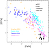 |
Fig. 2. [O/Fe]–[Fe/H] relation for the ICM and the Galaxy. The ICM Fe abundances and O/Fe abundance ratios (Table 1) are shown as black dots with (statistical) error bars.The Galactic Fe abundances and O/Fe abundance ratios are taken from Israelian et al. (2004; halo, orange), Reddy et al. (2006; disc and halo, cyan), Fabbian et al. (2009; halo, blue), and Nissen et al. (2014; disc and halo, pink). |
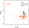 |
Fig. 3. Similar to Fig. 2, but for the [N/Fe]–[Fe/H] relation. The Galactic Fe abundances and N/Fe abundance ratios are taken from Shi et al. (2002), disc, red triangles) and Israelian et al. (2004), halo, orange diamonds) . |
For the [O/Fe]–[Fe/H] relation (Fig. 2), a gradual decrease of [O/Fe] with increasing [Fe/H] is found in the [Fe/H] ≲ –1 regime. The reason is that the more metal-poor the SNcc progenitor, the higher the [O/Fe] ratio in the SNcc (Romano et al. 2010). The rapid decrease of [O/Fe] in the [Fe/H] ≳ –1 regime, on the other hand, stems from the Fe enrichment by SNIa. The [O/Fe] ratio of the ICM is slightly lower than that of disc stars in the Galaxy with the same [Fe/H] ratio. The overall [O/Fe]–[Fe/H] relation of the ICM and the Galaxy still supports the idea that they share the same enrichment channel (SNcc plus SNIa) for O and Fe.
In contrast to the decreasing trend of [O/Fe] with increasing [Fe/H], a relatively flat [N/Fe] ratio with increasing [Fe/H] is found in Fig. 3, which indicates that N and O are enriched through different channels. The [N/Fe]–[Fe/H] relation for the disc and halo stars can be explained (see Fig. 3 in Romano et al. 2010) with AGB yields from Karakas (2010). The [N/Fe] ratio of the ICM is slightly higher than that of halo stars in the Galaxy with the same [Fe/H] ratio. The overall [N/Fe]–[Fe/H] relation of the ICM and the Galaxy indicates that they share the same enrichment channel (AGB) for N.
Secondly, we compare the [N/O]–[O/Fe] relation of supernova yields (Fig. 4) to the observed abundances (Fig. 5). The [O/Fe] ratio of the ICM is lower than that of halo stars since the ICM is enriched by both SNcc and SNIa, while halo stars are mainly enriched by SNcc. Generally speaking, the [N/O] ratio in the ICM is higher than that of halo stars. Similar results have been reported in Werner et al. (2006a) for M 87.
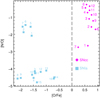 |
Fig. 4. TDiamonds (magenta) represent the IMF-weighted yields of SNcc (and PISNe for Zinit = 0), while the squares (blue) show SNIa yields. The indices next to the symbols indicate the corresponding model dependency (Tables 3 and 4). The yields of all the elements from C to Zn can be found in Figs. D.1 and D.2. |
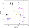 |
Fig. 5. Similar to Fig. 2, but for [N/O] vs. [O/Fe]. The results for Galactic stellar populations are taken from Israelian et al. (2004), Spite et al. (2005; halo, diamonds). The magenta box indicates the region of SNcc yields except for Zinit = 0, while the blue box indicates the region of SNIa yields (Fig. 4). |
If the chemical enrichment were completely due to massive stars ( in Eq. (3)), then we would have [O/Fe] ≳ 0.5 (Fig. 4), except for Zinit = 0. For Zinit = 0, the [O/Fe] ratio can be lower than ∼0.5 because of the explosive O-burning by PISNe (Nomoto et al. 2013). In Fig. 4 we assume that all the very massive stars undergo PISNe (Sect. 5.1). In reality, the exact value of [O/Fe] (for Zinit = 0) might differ, depending on the IMF and the fraction of very massive stars that undergo PISNe. The [O/Fe] ratios in the ICM (Fig. 5) are in the range of (–0.5, 0.2), suggesting that the enrichment from SNIa is required for the ICM, unless PISNe contributes significantly.
The nitrogen enrichment through SNIa is negligible ([N/O] ≲ –1). Therefore, one would expect [N/O] ≲ –0.2 (Fig. 4), if the chemical enrichment were completely due to massive stars ( in Eq. (3)). We caution that the [N/O] ratio for Zinit = 0 in Fig. 4 is in fact a lower limit, since we do not include enrichment from metal-poor rotating massive stars before they explode as supernovae, which is due to the lack of knowledge of corresponding number fraction and yields. Chiappini et al. (2006) have shown that a contribution as high as [N/Fe] ∼ 0.5 from metal-poor ([Fe/H] ≲ –2.5) rotating massive stars is required to solve the primary nitrogen problem (see also Fig. 3 in Romano et al. 2010). For a Salpeter IMF, the upper limit of [N/O] is estimated to be zero, given that not all the metal-poor massive stars are rotating (thus [N/Fe] ≲ 0.5) and [O/Fe] ≳ 0.5 (Fig. 4), regardless of Zinit. The same upper limit of [N/O] holds for a top-heavy IMF with Zinit ≳ 0.001. Nonetheless, for a top-heavy IMF with Zinit ≲ 0.001, the upper limit of [N/O] might be above zero, since [O/Fe] ratio can be lower than 0.5, as discussed previously.
The [N/O] ratios in the ICM are above zero at the ≳2.5σ confidence level (Table 1), indicating that in a Salpeter IMF, the massive stars cannot be the main nitrogen factory. In this case, nitrogen mainly originates from low- and intermediate-mass stars (AGBs). Nevertheless, we cannot rule out that in a top-heavy IMF with a low initial metallicity (Zinit ≲ 0.001), massive stars could be an important nitrogen enrichment factory.
Last but not least, we caution that the measured [N/Fe] and [N/O] ratios in Table 1 might be biased. The limited field of view (FOV) of the RGS means that the abundance ratios obtained in the rather small (≲0.05r500) extraction regions do not necessarily represent the abundance patterns within the closed-box scenario (Sect. 1). If the elements enriched through different channels were distributed in the ICM in different ways, so that, for instance, N were more centrally peaked than Fe and O, the resulting [N/Fe] and [N/O] ratios in the core region would appear to be higher.
5.3. Odd-Z elements
Previous studies of chemical enrichment in the ICM mainly focused on determining the SNIa fraction with respect to the total number of SNe that enriched the ICM (e.g. de Plaa et al. 2006). In terms of elemental abundances, most abundant even-Z elements from oxygen up to and including nickel (except Ti) have been measured. Additionally, one odd-Z Fe-peak element, Mn, is also studied in the stacked spectra of the CHEERS sample (Mernier et al. 2016a). In terms of the yields table, in addition to SNcc and SNIa, Pop III stars (Werner et al. 2006b; de Plaa et al. 2006) and Ca-rich gap transients (CaRGT, Mulchaey et al. 2014) have also been taken into account to interpret the observed abundance pattern. In this section, we include the nitrogen abundance and yields from AGBs (Campbell & Lattanzio 2008; Karakas 2010; Nomoto et al. 2013) for the chemical enrichment study of the ICM.
Since the number of abundance ratios derived from the RGS spectra are rather limited because the coverage of the energy range is relatively small, it is more meaningful when the abundance ratios measured with EPIC are also taken into account. Ideally, the abundances within ∼r500 of the ICM should be obtained so that the closed-box assumption is valid for massive clusters (Sect. 1). In practice, especially for groups of galaxies, the FOV of RGS merely covers a tiny fraction of r500. Moreover, the unknown nitrogen abundance gradients within r500 prevent us from extrapolating the abundances out to r500 with the obtained RGS abundances by hand.
We used both the RGS and EPIC results of NGC 5044 (Table 5) for the exercise here, given that the measurement uncertainty of the nitrogen abundance is typical (neither too large nor too small), and the extraction regions are comparable (∼0.034r500 for RGS and ∼0.05r500 for EPIC). In Table 5 the N/Fe, O/Fe, Ne/Fe, Mg/Fe, and Ni/Fe abundance ratios are measured with RGS, while the Si/Fe, S/Fe, Ar/Fe, and Ca/Fe ratios are measured with EPIC (see details in Appendix C).
Abundance ratios for NGC 5044 within the extraction region (i.e. ≲r/r500).
We emphasise that we focus on the comparison among different settings of the ICM enrichment model, that is, the choice of IMF index and the initial metallicity of the stellar population, the choice of SNIa model, and whether to include enrichment from AGBs.
It is possible that SNIa from different channels (through single- or double-degenerate, deflagration or detonation, and super- or sub-Chandrasekhar limit) all play a role in the chemical enrichment of the ICM (Finoguenov et al. 2002; Mernier et al. 2016b). We only fit the measured abundance ratios with one set of SNIa yields for simplicity. Including an additional set of Ca-rich gap transient yields improves the statistics negligibly and does not change the above main points.
Since almost all the measured abundance ratios (Table 5) are close to solar, we restricted the initial metallicity of the stellar populations to be solar and sub-solar (i.e. excluding Zinit = 0.05). Thus, the observed abundance ratios were fitted to 10 (2 sets of IMF and 5 sets of Zinit) × 16 (for SNIa) combinations of yield tables. The reduced chi-squared ( ) for all the fits are shown in the upper panel of Fig. 6. The 10 × 16 combinations of the chemical enrichment models are highly degenerate. We can reject many combinations based on the statistics, for example,
  , that is,
  , but the IMF power-law index and SNIa models cannot be exclusively obtained with current abundance measurements.
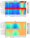 |
Fig. 6. Colour map of reduced chi-squared (χ2/d.o.f. in log10 scale, upper panel) and SNIa fraction ( |

Typical best fits of the abundance ratios in NGC 5044 to stellar yields are shown in Fig. 7 (without the N/Fe ratio and yields from AGBs) and Fig. 8 (with the N/Fe ratio and yields from AGBs). Without yields from AGBs (Fig. 7), we also show the model prediction on the N/Fe ratio (∼0.2). Compared to the measured N/Fe ratio (1.4 ± 0.3), the predicted N/Fe ratio is lower by ∼4σ, indicating that the contribution from SNcc is not enough to explain the observed N/Fe ratio. When we include yields from AGBs (Fig. 8), the predicted N/Fe ratio is consistent (≲1σ) with the observed N/Fe ratio. Additionally, the predicted O/Fe ratio decreases from ∼0.69 (SNe) to ∼0.66 (SNe + AGBs) as a result of the negative oxygen yields in AGBs.
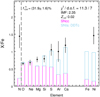 |
Fig. 7. One of the acceptable fits of chemical enrichment in NGC 5044. Yields of SNcc (magenta) and SNIa (blue) are used for the fit with Eq. (5). The adopted IMF power-law index is 2.35 (Salpeter) and the initial metallicity of the stellar population is 0.02 (solar). N/Fe and yields of AGBs are not included in the fit, but are shown for comparison. The SNIa fraction |
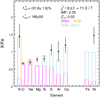 |
Fig. 8. Similar to Fig. 7, but N/Fe and AGB yields (orange) are included during the fit. Again, the favoured IMF power-law index is 2.35 (Salpeter) and Zinit = 0.02. The SNIa fraction is consistent with the previous result. The ratio ( |

In most cases, a Salpeter IMF provides better χ2 statistics (Fig. 6). When a Salpeter IMF and DDTc SNIa model are adopted, the SNIa fraction ( ) is consistent with ∼32%, regardless of whether we include N/Fe and AGBs enrichment (Figs. 7 and 8). The ratio (
 ) between the number of low- and intermediate-mass stars and that of massive stars is 180 ± 50. In a Salpeter IMF, the ratio (
 ) is expected to be ∼40, which is lower than the fitted value by ∼3σ. Again, the closed-box assumption is not fulfilled here, so that if the AGB products were more centrally peaked than the SNcc products (Sect. 5.2), a higher
  obtained here could be explained.
When N/Fe and AGB enrichment are not included in the fit, the best-fit initial metallicity is 0.02 (solar). This is mainly constrained by the lower-than-unity O/Mg abundance ratio (Fig. 9). Including N/Fe and AGB enrichment again favours solar initial metallicity. We also note that in both cases, a wide range of Zinit yields comparable results (Table 6), except for Zinit = 0.
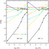 |
Fig. 9. IMF-weighted abundance ratios (with respect to Mg) as a function of the initial metallicity of massive stars (the SNcc channel). The results for Zinit = 0 are plotted at ∼ − 3.3. |
Best fits (d.o.f. = 7) of chemical enrichment in NGC 5044, given the IMF power-law index and initial metallicity of the stellar population.
In principle, when odd-Z elemental abundances, such as nitrogen, are included in the analysis, the initial metallicity of the stellar population should be better constrained, since yields of odd-Z elements increase significantly with increasing Zinit owing to a surplus of neutrons (Nomoto et al. 2013), while those of even-Z and Fe-peak elements are almost constant over a wide range of metallicities. This is shown clearly in Fig. 9 for massive stars. We emphasise that the denominator of the abundance ratio on the Y-axis is set to Mg instead of Fe in Fig. 9. This is because Mg enrichment through SNIa and AGBs are negligible, so that the observed abundance ratios of Na/Mg and Al/Mg can be used directly to probe the initial metallicity of the stellar population.
For future work, more accurate abundance measurements of odd-Z elements including N, Na, and/or Al are required to better constrain the initial metallicity of the stellar population. Current instruments lack the spectral resolution to resolve the Lyα lines of Na XI and Al XIII. Hopefully, future missions with high spectral resolution and large effective area like XARM (X-ray astronomy recovery mission) and Athena (Nandra et al. 2013) will address these issues.
6. Conclusions
We constrained the N/Fe ratio in the core (r/r500 ≲ 0.5) of one cluster (A 3526) and seven groups of galaxies (M 49, M 87, NGC 4636, NGC 4649, NGC 5044, NGC 5813, and NGC 5846) in the CHEERS sample with high-resolution RGS spectra. Our main conclusions are summarised as follows:
-
The nitrogen abundance is well constrained (≳3σ) in objects with a relatively cool ICM (kT ≲ 2 keV). For some of the systems (e.g. NGC 3411) in the CHEERS sample, more exposure time is required to better constrain the nitrogen abundance. In objects with a hotter ICM (kT ≳ 2 − 3 keV), the continuum level is high so that weak emission lines such as the N VII Lyα cannot be well constrained.
-
Both the [O/Fe]–[Fe/H] and [N/Fe]–[Fe/H] relations observed in the ICM are comparable to those observed in different stellar populations in the Galaxy, indicating that the enrichment channels for N, O, and Fe are expected to be the same. One possible explanation for the super solar N/Fe and N/O ratios in the ICM is the bias introduced by our small extraction region (r < 0.05r500). This potential bias can be confirmed by radial abundance maps for N, O, and Fe in future work.
-
If the observed ratio [N/O] > 0 (at the ≳2.5σ confidence level) is not biased because of the small extraction region, the low- and intermediate-mass stars are found to be the main metal factory for nitrogen in a Salpeter IMF. This is in agreement with the Galactic chemical evolution theory and previous studies of M 87. Nitrogen enrichment from massive stars might still be important, especially if the stellar population were to have a top-heavy IMF and zero initial metallicity.
-
We find that the obtained SNIa fraction is insensitive to the N abundance and AGB yields.
-
We also point out that accurate abundance measurements of odd-Z, such as N, Na, and Al, can certainly help to better constrain the initial metallicity of the stellar population that enriched the ICM.
The radius within which the plasma mass density is 500 times the critical density of the Universe at the redshift of the groups and clusters of galaxies.
![Mathematical equation: $ \left[\mathrm{A}/\mathrm{B} \right]_{\mathrm{ICM / star}} = \log_{10}\left(\frac{N_{\mathrm{A}}}{N_{\mathrm{B}}}\right)_{\mathrm{ICM / star}} - \log_{10}\left(\frac{N_{\mathrm{A}}}{N_{\mathrm{B}}}\right)_{\odot} =\log_{10}\left(\frac{Z_{\mathrm{A}}}{Z_{\mathrm{B}}}\right)_{\mathrm{ICM / star}} $](/articles/aa/full_html/2019/01/aa30931-17/aa30931-17-eq23.gif) .
.
We refer to the http://var.sron.nl/SPEX-doc/manualv3.04.00.pdf SPEX manual for more details on the SPEX Atomic Code & Tables.
Acknowledgments
This paper is dedicated to the memory of our highly regarded colleague Yu-Ying Zhang, who recently passed away. This work is based on the XMM-Newton AO-12 proposal (ID: 72380) “The XMM-Newton view of chemical enrichment in bright galaxy clusters and groups” (PI: de Plaa). The observations are obtained with XMM-Newton, an ESA science mission with instruments and contributions directly funded by ESA member states and the USA (NASA). SRON is supported financially by NWO, the Netherlands Organization for Scientific Research. J. M. grateful acknowledges discussions and consultations with C. de Vries, J. Sanders and O. Pols. C.P. acknowledges support from ERC Advanced Grant Feedback 340442. Y. Y. Z. acknowledges support by the German BMWi through the Verbundforschung under grant 50OR1506. H. A. acknowledges the support of NWO via a Veni grant.
References
- Anders, E., & Grevesse, N. 1989, Geochim. Cosmochim. Acta, 53, 197 [Google Scholar]
- Asplund, M. 2005, ARA&A, 43, 481 [NASA ADS] [CrossRef] [Google Scholar]
- Badenes, C., Borkowski, K. J., Hughes, J. P., Hwang, U., & Bravo, E. 2006, ApJ, 645, 1373 [NASA ADS] [CrossRef] [Google Scholar]
- Badnell, N. R. 2006, ApJS, 167, 334 [NASA ADS] [CrossRef] [Google Scholar]
- Barkat, Z., Rakavy, G., & Sack, N. 1967, Phys. Rev. Lett., 18, 379 [NASA ADS] [CrossRef] [Google Scholar]
- Böhringer, H., & Werner, N. 2010, A&ARv, 18, 127 [NASA ADS] [CrossRef] [Google Scholar]
- Buote, D. A. 2000, MNRAS, 311, 176 [NASA ADS] [CrossRef] [Google Scholar]
- Buote, D. A., & Canizares, C. R. 1994, ApJ, 427, 86 [NASA ADS] [CrossRef] [Google Scholar]
- Bulbul, E., Smith, R. K., & Loewenstein, M. 2012, ApJ, 753, 54 [NASA ADS] [CrossRef] [Google Scholar]
- Campbell, S. W., & Lattanzio, J. C. 2008, A&A, 490, 769 [NASA ADS] [CrossRef] [EDP Sciences] [Google Scholar]
- Chandrasekhar, S. 1931, MNRAS, 91, 456 [NASA ADS] [CrossRef] [Google Scholar]
- Chen, Y., Reiprich, T. H., Böhringer, H., Ikebe, Y., & Zhang, Y.-Y. 2007, A&A, 466, 805 [NASA ADS] [CrossRef] [EDP Sciences] [Google Scholar]
- Chiappini, C., Hirschi, R., Meynet, G., et al. 2006, A&A, 449, L27 [NASA ADS] [CrossRef] [EDP Sciences] [Google Scholar]
- Churazov, E., Forman, W., Jones, C., & Böhringer, H. 2003, ApJ, 590, 225 [NASA ADS] [CrossRef] [Google Scholar]
- de Plaa, J., Kaastra, J. S., Tamura, T., et al. 2004, A&A, 423, 49 [NASA ADS] [CrossRef] [EDP Sciences] [Google Scholar]
- de Plaa, J., Werner, N., Bykov, A. M., et al. 2006, A&A, 452, 397 [NASA ADS] [CrossRef] [EDP Sciences] [Google Scholar]
- de Plaa, J., Kaastra, J. S., Werner, N., et al. 2017, A&A, 607, A98 [NASA ADS] [CrossRef] [EDP Sciences] [Google Scholar]
- den Herder, J. W., Brinkman, A. C., Kahn, S. M., et al. 2001, A&A, 365, L7 [NASA ADS] [CrossRef] [EDP Sciences] [Google Scholar]
- Fabbian, D., Nissen, P. E., Asplund, M., Pettini, M., & Akerman, C. 2009, A&A, 500, 1143 [NASA ADS] [CrossRef] [EDP Sciences] [Google Scholar]
- Finoguenov, A., Matsushita, K., Böhringer, H., Ikebe, Y., & Arnaud, M. 2002, A&A, 381, 21 [NASA ADS] [CrossRef] [EDP Sciences] [Google Scholar]
- Frank, K. A., Peterson, J. R., Andersson, K., Fabian, A. C., & Sanders, J. S. 2013, ApJ, 764, 46 [NASA ADS] [CrossRef] [Google Scholar]
- Fujita, Y., Tawa, N., Hayashida, K., et al. 2008, PASJ, 60, S343 [NASA ADS] [CrossRef] [Google Scholar]
- Gil-Pons, P., Gutiérrez, J., & García-Berro, E. 2007, A&A, 464, 667 [NASA ADS] [CrossRef] [EDP Sciences] [Google Scholar]
- Grange, Y. G., de Plaa, J., Kaastra, J. S., et al. 2011, A&A, 531, A15 [NASA ADS] [CrossRef] [EDP Sciences] [Google Scholar]
- Greene, J. E., Janish, R., Ma, C.-P., et al. 2015, ApJ, 807, 11 [NASA ADS] [CrossRef] [Google Scholar]
- Gu, M. F. 2008, Can. J. Phys., 86, 675 [NASA ADS] [CrossRef] [Google Scholar]
- Henriques, B. M. B., White, S. D. M., Thomas, P. A., et al. 2015, MNRAS, 451, 2663 [NASA ADS] [CrossRef] [Google Scholar]
- Herwig, F. 2005, ARA&A, 43, 435 [NASA ADS] [CrossRef] [Google Scholar]
- Hitomi Collaboration (Aharonian, F., et al.) 2017, Nature, 551, 478 [NASA ADS] [CrossRef] [Google Scholar]
- Hitomi Collaboration (Aharonian, F., et al.) 2018, PASJ, 70, 12 [NASA ADS] [Google Scholar]
- Iben, Jr., I., & Renzini, A. 1983, ARA&A, 21, 271 [NASA ADS] [CrossRef] [Google Scholar]
- Israelian, G., Ecuvillon, A., Rebolo, R., et al. 2004, A&A, 421, 649 [NASA ADS] [CrossRef] [EDP Sciences] [Google Scholar]
- Iwamoto, K., Brachwitz, F., Nomoto, K., et al. 1999, ApJS, 125, 439 [NASA ADS] [CrossRef] [MathSciNet] [Google Scholar]
- Johansson, J., Thomas, D., & Maraston, C. 2012, MNRAS, 421, 1908 [NASA ADS] [CrossRef] [Google Scholar]
- Kaastra, J. S. 2017, A&A, 605, A51 [NASA ADS] [CrossRef] [EDP Sciences] [Google Scholar]
- Kaastra, J. S., & Bleeker, J. A. M. 2016, A&A, 587, A151 [NASA ADS] [CrossRef] [EDP Sciences] [Google Scholar]
- Kaastra, J. S., Mewe, R., & Nieuwenhuijzen, H. 1996, Lab. Plasmas, 411 [Google Scholar]
- Kaastra, J. S., Paerels, F. B. S., Durret, F., Schindler, S., & Richter, P. 2008, Space Sci. Rev., 134, 155 [NASA ADS] [CrossRef] [Google Scholar]
- Kaastra, J. S., Lanz, T., Hubeny, I., & Paerels, F. B. S. 2009, A&A, 497, 311 [NASA ADS] [CrossRef] [EDP Sciences] [Google Scholar]
- Karakas, A. I. 2010, MNRAS, 403, 1413 [NASA ADS] [CrossRef] [Google Scholar]
- Kobayashi, C., Umeda, H., Nomoto, K., Tominaga, N., & Ohkubo, T. 2006, ApJ, 653, 1145 [NASA ADS] [CrossRef] [Google Scholar]
- Komiyama, M., Sato, K., Nagino, R., Ohashi, T., & Matsushita, K. 2009, PASJ, 61, S337 [NASA ADS] [Google Scholar]
- Landry, D., Bonamente, M., Giles, P., et al. 2013, MNRAS, 433, 2790 [NASA ADS] [CrossRef] [Google Scholar]
- Lodders, K., Palme, H., & Gail, H.-P. 2009, Landolt Börnstein, 44 [Google Scholar]
- Loewenstein, M. 2013, ApJ, 773, 52 [NASA ADS] [CrossRef] [Google Scholar]
- Maeda, K., Röpke, F. K., Fink, M., et al. 2010, ApJ, 712, 624 [NASA ADS] [CrossRef] [Google Scholar]
- Mao, J., & Kaastra, J. 2016, A&A, 587, A84 [NASA ADS] [CrossRef] [EDP Sciences] [Google Scholar]
- Mernier, F., de Plaa, J., Lovisari, L., et al. 2015, A&A, 575, A37 [Google Scholar]
- Mernier, F., de Plaa, J., Pinto, C., et al. 2016a, A&A, 592, A157 [NASA ADS] [CrossRef] [EDP Sciences] [Google Scholar]
- Mernier, F., de Plaa, J., Pinto, C., et al. 2016b, A&A, 595, A126 [NASA ADS] [CrossRef] [EDP Sciences] [Google Scholar]
- Mernier, F., de Plaa, J., Kaastra, J. S., et al. 2017, A&A, 603, A80 [NASA ADS] [CrossRef] [EDP Sciences] [Google Scholar]
- Mernier, F., de Plaa, J., Werner, N., et al. 2018, MNRAS, 478, L116 [NASA ADS] [CrossRef] [Google Scholar]
- Mollá, M., Cavichia, O., Gavilán, M., & Gibson, B. K. 2015, MNRAS, 451, 3693 [NASA ADS] [CrossRef] [Google Scholar]
- Mulchaey, J. S., Kasliwal, M. M., & Kollmeier, J. A. 2014, ApJ, 780, L34 [NASA ADS] [CrossRef] [Google Scholar]
- Nandra, K., Barret, D., Barcons, X. et al. 2013, ArXiv e-prints [arXiv:1306.2307] [Google Scholar]
- Nissen, P. E., Chen, Y. Q., Carigi, L., Schuster, W. J., & Zhao, G. 2014, A&A, 568, A25 [NASA ADS] [CrossRef] [EDP Sciences] [Google Scholar]
- Nomoto, K., Kobayashi, C., & Tominaga, N. 2013, ARA&A, 51, 457 [NASA ADS] [CrossRef] [Google Scholar]
- Pinto, C., Sanders, J. S., Werner, N., et al. 2015, A&A, 575, A38 [NASA ADS] [CrossRef] [EDP Sciences] [Google Scholar]
- Pinto, C., Fabian, A. C., Ogorzalek, A., et al. 2016, MNRAS, 461, 2077 [NASA ADS] [CrossRef] [Google Scholar]
- Pipino, A., Devriendt, J. E. G., Thomas, D., Silk, J., & Kaviraj, S. 2009, A&A, 505, 1075 [NASA ADS] [CrossRef] [EDP Sciences] [Google Scholar]
- Pols, O. R., Izzard, R. G., Stancliffe, R. J., & Glebbeek, E. 2012, A&A, 547, A76 [NASA ADS] [CrossRef] [EDP Sciences] [Google Scholar]
- Reddy, B. E., Lambert, D. L., & Allende Prieto, C. 2006, MNRAS, 367, 1329 [NASA ADS] [CrossRef] [Google Scholar]
- Renzini, A., & Andreon, S. 2014, MNRAS, 444, 3581 [NASA ADS] [CrossRef] [Google Scholar]
- Romano, D., Chiappini, C., Matteucci, F., & Tosi, M. 2005, A&A, 430, 491 [NASA ADS] [CrossRef] [EDP Sciences] [Google Scholar]
- Romano, D., Karakas, A. I., Tosi, M., & Matteucci, F. 2010, A&A, 522, A32 [NASA ADS] [CrossRef] [EDP Sciences] [Google Scholar]
- Salpeter, E. E. 1955, ApJ, 121, 161 [Google Scholar]
- Sanders, J. S., & Fabian, A. C. 2006, MNRAS, 371, 1483 [NASA ADS] [CrossRef] [Google Scholar]
- Sanders, J. S., & Fabian, A. C. 2011, MNRAS, 412, L35 [NASA ADS] [CrossRef] [Google Scholar]
- Sanders, J. S., Fabian, A. C., Allen, S. W., et al. 2008, MNRAS, 385, 1186 [NASA ADS] [CrossRef] [Google Scholar]
- Sanders, J. S., Fabian, A. C., Frank, K. A., Peterson, J. R., & Russell, H. R. 2010, MNRAS, 402, 127 [NASA ADS] [CrossRef] [Google Scholar]
- Sanders, J. S., Fabian, A. C., & Smith, R. K. 2011, MNRAS, 410, 1797 [NASA ADS] [Google Scholar]
- Saro, A., Borgani, S., Tornatore, L., et al. 2006, MNRAS, 373, 397 [NASA ADS] [CrossRef] [Google Scholar]
- Sato, K., Tokoi, K., Matsushita, K., et al. 2007, ApJ, 667, L41 [NASA ADS] [CrossRef] [Google Scholar]
- Schindler, S., & Diaferio, A. 2008, Space Sci. Rev., 134, 363 [NASA ADS] [CrossRef] [Google Scholar]
- Shi, J. R., Zhao, G., & Chen, Y. Q. 2002, A&A, 381, 982 [NASA ADS] [CrossRef] [EDP Sciences] [Google Scholar]
- Siess, L. 2007, A&A, 476, 893 [NASA ADS] [CrossRef] [EDP Sciences] [Google Scholar]
- Simionescu, A., Roediger, E., Nulsen, P. E. J., et al. 2009, A&A, 495, 721 [NASA ADS] [CrossRef] [EDP Sciences] [Google Scholar]
- Smith, R. K., Brickhouse, N. S., Liedahl, D. A., & Raymond, J. C. 2001, ApJ, 556, L91 [NASA ADS] [CrossRef] [Google Scholar]
- Smith, R. J., Lucey, J. R., Hudson, M. J., & Bridges, T. J. 2009, MNRAS, 398, 119 [NASA ADS] [CrossRef] [Google Scholar]
- Spite, M., Cayrel, R., Plez, B., et al. 2005, A&A, 430, 655 [NASA ADS] [CrossRef] [EDP Sciences] [Google Scholar]
- Steenbrugge, K. C., Kaastra, J. S., Crenshaw, D. M., et al. 2005, A&A, 434, 569 [NASA ADS] [CrossRef] [EDP Sciences] [Google Scholar]
- Tamura, T., Bleeker, J. A. M., Kaastra, J. S., Ferrigno, C., & Molendi, S. 2001, A&A, 379, 107 [NASA ADS] [CrossRef] [EDP Sciences] [Google Scholar]
- Tamura, T., Kaastra, J. S., Makishima, K., & Takahashi, I. 2003, A&A, 399, 497 [NASA ADS] [CrossRef] [EDP Sciences] [Google Scholar]
- Tamura, T., Kaastra, J. S., den Herder, J. W. A., Bleeker, J. A. M., & Peterson, J. R. 2004, A&A, 420, 135 [NASA ADS] [CrossRef] [EDP Sciences] [Google Scholar]
- Umeda, H., & Nomoto, K. 2002, ApJ, 565, 385 [NASA ADS] [CrossRef] [Google Scholar]
- Urdampilleta, I., Kaastra, J. S., & Mehdipour, M. 2017, A&A, 601, A85 [NASA ADS] [CrossRef] [EDP Sciences] [Google Scholar]
- Walker, S. A., Fabian, A. C., Sanders, J. S., George, M. R., & Tawara, Y. 2012, MNRAS, 422, 3503 [NASA ADS] [CrossRef] [Google Scholar]
- Werner, N., Böhringer, H., Kaastra, J. S., et al. 2006a, A&A, 459, 353 [NASA ADS] [CrossRef] [EDP Sciences] [Google Scholar]
- Werner, N., de Plaa, J., Kaastra, J. S., et al. 2006b, A&A, 449, 475 [NASA ADS] [CrossRef] [EDP Sciences] [Google Scholar]
- Werner, N., Durret, F., Ohashi, T., Schindler, S., & Wiersma, R. P. C. 2008, Space Sci. Rev., 134, 337 [NASA ADS] [CrossRef] [Google Scholar]
- Werner, N., Zhuravleva, I., Churazov, E., et al. 2009, MNRAS, 398, 23 [NASA ADS] [CrossRef] [Google Scholar]
- Werner, N., Urban, O., Simionescu, A., & Allen, S. W. 2013, Nature, 502, 656 [NASA ADS] [CrossRef] [Google Scholar]
- White, S. D. M., Navarro, J. F., Evrard, A. E., & Frenk, C. S. 1993, Nature, 366, 429 [NASA ADS] [CrossRef] [Google Scholar]
- Willingale, R., Starling, R. L. C., Beardmore, A. P., Tanvir, N. R., & O’Brien, P. T. 2013, MNRAS, 431, 394 [NASA ADS] [CrossRef] [Google Scholar]
- Xu, H., Kahn, S. M., Peterson, J. R., et al. 2002, ApJ, 579, 600 [NASA ADS] [CrossRef] [Google Scholar]
- Zhang, Y.-Y., Andernach, H., Caretta, C. A., et al. 2011, A&A, 526, A105 [NASA ADS] [CrossRef] [EDP Sciences] [Google Scholar]
- Zijlstra, A. A. 2004, MNRAS, 348, L23 [NASA ADS] [CrossRef] [MathSciNet] [Google Scholar]
Appendix A: Global spectral fit
The global fits to the 7–28 Å wavelength range for each source in Table 1 are shown in Fig. A.1. The locations (in the observed frame) of characteristic emission lines are labelled, including the Lyα line from H-like N VII, O VIII, Ne X, Mg XII, He-like triplets from O VII, Ne IX, Mg XI, and the resonance and forbidden lines of Ne-like Fe XVII.
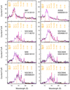 |
Fig. A.1. Global fits to the 7–28 Å wavelength range. The data points are shown in black (RGS1) and grey (RGS2), and the model spectra are shown in red (RGS1) and magenta (RGS2) histograms. Spectra from only one observation per target are shown for clarity. |
Appendix B: Systematic uncertainties in spectral analysis
B.1. Differential emission measure distribution
Fitting a multi-temperature plasma with a single-temperature (1T) model would often over-estimate the emission measure and under-estimate the abundances (Buote & Canizares 1994; Buote 2000). Alternatively, a two-temperature (2T) or multi-temperature (GDEM) model can measure the nitrogen abundance more accurately.
If the emission measure of the hotter component is ≳5 times that of the cooler one, the N VII in the hotter CIE component in a 2T model contributes more to the observed N VII Lyα emission in the spectra. Given the same emission measure and nitrogen abundance, the N VII Lyα line flux is proportional to the N VII ion concentration (relative to all the nitrogen atoms and ions in the ICM) times the level occupations of 2P0.5 and 2P1.5 (the sum of occupations of all the levels is defined as unity). As the level occupations increase gradually as a function of plasma temperature (bottom panel in Fig. B.1), the N VII ion concentration is the leading factor to determine the line emissivity. As mentioned above, we tied the abundances in our 2T model, thus, assuming kTc ≲ 0.7 keV and kTh ≳ 2 keV, when Yc/Yh ≲ 0.2, the N VII in the hotter component contributes more to the emission line, while for Yc/Yh ≳ 0.2, the N VII is mainly from the cooler component.
In addition, the line emissivity of N VII Lyα peaks around T ∼ 2 × 10⁶ K (Kaastra et al. 2008), implying that nitrogen is preferably found in relatively cooler plasma. As the line emissivity declines rapidly with the increasing temperature of the plasma (top panel in Fig. B.1), we find that it is rather difficult to constrain the nitrogen abundance well through the extremely weak N VII Lyα emission line, which is embedded in the relatively high continuum where kT ≳ 2 − 3 keV.
B.2. Spatial broadening model
The spatial broadening model lpro is built based on the spatial broadening profile. The latter is obtained from the MOS1 image, since the MOS1 DETY direction is in parallel to the RGS1 dispersion direction. There are two more free parameters in lpro, the scaling factor (s) and the offset parameter. Here we discuss the systematic uncertainties of the spatial broadening model.
For instance, the bright non-thermal emission in the second observation (ObsID: 0200920101) means that not only the spectra are heavily contaminated in M 87, but the spatial broadening model created with the MOS1 image is also affected. The brighter the central non-thermal emission, the more centrally peaked the surface brightness profile (seen indirectly in Fig. B.3). Spatial broadening models built on these biased surface brightness profiles no longer reflect the proper spatial extent of the ICM.
We compare the (global) fit results using different line broadening profile of M 87 here. If the non-thermal emission were merely a point source and the ICM were azimuthally symmetric, one might fit the observed 2D image with two Gaussian or Lorentzian profiles with different widths, then subtract the non-thermal emission counterpart to obtain the profile for the ICM only. However, this is not the case for M 87 because of its azimuthal asymmetry (Fig. B.2). Because the emission centre is offset by ∼1.5 arcmin in 0200920101, we took advantage of a ∼1.6 arcmin wide extraction region without the non-thermal emission, leading to a better but still biased (probably flatter) spatial broadening model (Fig. B.3). In contrast, we found that the lpro scaling factor (free parameter) can account for the bias in the spatial broadening profile.
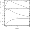 |
Fig. B.1. N VII Lyα line emissivity (top), relative ion concentration (middle), and relative level occupation (bottom) of the two upper levels 2P0.5 and 2P1.5 (in sum, since the fine-structure lines cannot be distinguished). The underlying ionisation balance of Urdampilleta et al. (2017) and the proto-solar abundance of Lodders et al. (2009) is used. In a hot (kT ≳ 0.6 keV) single-temperature CIE plasma, nitrogen is almost fully ionised in the form of N VIII, i.e. the ion concentration of N VIII is ∼1. Most of the N VII is in the ground level 1S0.5, i.e. the level occupations of 1S0.5 is close to unity. |
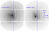 |
Fig. B.2. 7–28 Å energy band MOS1 image in the detector coordinate system for M 87. The MOS1 DETX axis is in parallel with the cross-dispersion direction (XDSP) of the RGS. In the second observation (0200920101), the non-thermal emission is much brighter, offset by ∼1.5 arcmin, and the image is rotated ∼188° clockwise. The (blue) rectangular boxes indicate the extraction regions for rgsvprof. For the first observation, a 99%-xpsf (∼3.4 arcmin) extraction region, aligned with the RGS source extraction region, is used. For the seconding observation, only the onset 95%-xpsf (∼1.6 arcmin) extraction region (to avoid central contamination) is shown for clarity. |
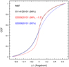 |
Fig. B.3. Cumulative distribution function of the spatial broadening profile of M 87. We built the spatial broadening profiles for both two observations (black and red) of the RGS 99%-xpsf source extraction regions. For the second observation (0200920101), a 1.5 arcmin offset is applied so that the extraction region is centred on the peak of the X-ray emission. Moreover, for the second observation, we also built a spatial broadening profile with a narrower 95%-xpsf extraction region (blue) that is less strongly affected by central contamination (Fig. B.2). |
Other than the accuracy of the spatial broadening profile, the scaling factors might be different for different thermal components and/or different ions within the same thermal component. When studying the O VII He-like triplets in the CHEERS sample, Pinto et al. (2016) found the spatial extent of the cooler ICM component is narrower than that of the hotter counterpart, by using two lpro model components for the two temperature components. Since in most cases, nitrogen from the hotter component contributes most to the emission line we observed, applying the same lpro model component (mainly determined by the high-temperature lines) to both the hotter and the cooler thermal component is therefore expected to be fine in our case.
B.3. RGS background model
In some cases in the CHEERS sample, the modelled background level is even higher than the source continuum level at λ ≳ 20 Å (Fig. 1). Thus we checked the systematic uncertainties of the modelled background as well. We used A 2029 as an example to compare the observed spectra from an offset observation toward A 2029 with the RGS-modelled background.
The outskirts of A 2029 were observed with XMM-Newton in 2015. The projected angular distances for the outskirts are ∼20 arcmin, that is, at least ∼1.3r500. The outskirts of A 2029 were also observed by Suzaku, and no statistically significant emission is detected beyond 22 arcmin, except for the northern observation (Walker et al. 2012). That is to say, the spectra of the observations toward the outskirts of A 2029 can be considered as background spectra. We used the same data-reduction method as described in Sect. 2 to screen out the flare-time intervals and extracted the RGS spectra in the 99% xpsf extraction region.
In Fig. B.4 we plot the RGS first-order net (observed minus modelled background) spectra of the A 2029 southern outskirt (ObsID: 0744411001). If the modelled background spectra is accurate enough, the net spectra should be consistent with zero. Above ∼26.5 Å, the modelled background spectrum of RGS1 is significantly over-estimated. The RGS2 modelled background is more accurate than that of RGS1 above ∼26.5 Å. Therefore, for any source with redshift z ≳ 0.07, the accuracy of the RGS1-modelled background can be an issue for the N VII Lyα line measurement, if the modelled background level dominates the source continuum level for (redshifted)λ ≳ 26.5 Å.
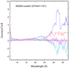 |
Fig. B.4. RGS first-order spectra of the A 2029 outskirt (ObsID: 0744411001). The data with error bars (light blue for RGS1 and violet for RGS2) are the observed background spectra minus the modelled background spectra, which are expected to be around zero if the modelled background spectra are accurate. The solid lines (deep blue for RGS1 and red for RGS2) are the (subtracted) modelled background spectra obtained with rgsproc. |
Last but not least, we take NGC 5846 as an example to show the impact on the abundance measurement if the modelled background were systematically over- or under-estimated. We used the FTOOL task fcalc to increase and decrease the values of the entire BACKSCAL column by 10% for the modelled background spectra FITS file. Then we re-analysed the source spectra after subtracting the modified modelled background spectra. Given a 2T model, compared to the results of unmodified modelled background (Table 1), the Fe abundance increases and decreases dramatically by +0.33 (for 90% BACKSCAL) and −0.15 (for 110% BACKSCAL), respectively. The deviations are significantly larger than pure statistical errors. Nevertheless, the abundance ratios of N/Fe and O/Fe are consistent with 3.4 and 1.3, respectively. That is to say, the abundance ratios are robust given a 10% (constant) uncertainty in the modelled background spectra. Similar checks were also performed on other sources with higher modelled background level.
Appendix C: EPIC spectral analysis of NGC 5044 with SPEX v3.03
The EPIC Si/Fe, S/Fe, Ar/Fe, and Ca/Fe abundance ratios (the dagger in Table 5) have been reported in Mernier et al. (2016a, their Table D.1). However, an older version of SPEX (v2.05) was used at that time. We here reanalysed the EPIC spectra with SPEX v3.03. As shown in Table C.1, the newly obtained abundance ratios are consistent (at a 1σ confidence level) with those reported in Mernier et al. (2016a).
Best-fit results of the EPIC spectra of NGC 5044 using SPEX v2.05 and v3.03.
More accurate and complete atomic data (SPEXACT v3.03)5 are used in SPEX v3.03 (Sect. 3). The total number of lines has increased by a factor of ∼400 to reach about 1.8 million in the new version. Consequently, multi-temperature plasma models such as the GDEM, which has about 20 different normalisation and temperature components, is computationally expensive for SPEX v3.03. A three-temperature (3T) model would be a cheaper alternative for SPEX v3.03. To mimic a Gaussian differential emission measure distribution (GDEM) with a three-temperature distribution, we let the temperatures of all three components vary, the normalisation of the main component was also allowed to vary, while the normalisation of the low- and high-temperature components were fixed to be half of that of the main component (see also Mernier et al. 2018).
MOS and pn spectra were fitted simultaneously. When we used the old atomic database (SPEXACT v2.05), the ratios of the best-fit C-statistics to d.o.f. are 6502/1512 (GDEM in SPEX v2.05) and 6210/1287 (3T in SPEX v3.03). As expected, the ratio is slightly lower for the 3T model. The degrees of freedoms are different mainly because the optimal binning algorithm (Kaastra & Bleeker 2016) is different in the two versions of SPEX.
When we used the 3T model and SPEX v3.03, the ratios of the best-fit C-statistiscs to d.o.f. are 6210/1287 (SPEXACT v2.05) and 5635/1287 (SPEXACT v3.03). This shows the improvement that is reached with the new atomic data.
Appendix D: IMF weighted SNcc yields and yields of SNIa.
The IMF-weighted SNcc yields are shown in Fig. D.1 with different initial metallicity (Zinit) and IMF for the stellar progenitors. The yields table of Nomoto et al. (2013) was used for the calculation. Figure D.2 shows the SNIa yields based on theoretical calculations (Iwamoto et al. 1999) and observations of the Tycho supernova remnant (Badenes et al. 2006).
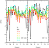 |
Fig. D.1. IMF-weighted SNcc yields, based on the yields table of Nomoto et al. (2013). |
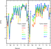 |
Fig. D.2. Yields from various SNIa models (Iwamoto et al. 1999; Badenes et al. 2006). |
All Tables
Abundances and abundance ratios within the 3.4 arcmin wide (in the cross-dispersion direction) extraction region.
Best fits (d.o.f. = 7) of chemical enrichment in NGC 5044, given the IMF power-law index and initial metallicity of the stellar population.
All Figures
|
Fig. 1. Observed RGS spectra in the N VII neighbourhood, i.e., 23–28 Å wavelength range. The data points are shown in black (RGS1) and grey (RGS2), the modelled background spectra are shown in deep blue (RGS1) and light blue (RGS2) histograms, and the (global fit) model spectra are shown in red (RGS1) and magenta (RGS2) histograms. Vertical dashed lines indicate the O VIII Lyα around 19 Å and N VII Lyα around 25 Å in the observed frame. Spectra from merely one observation per target are shown for clarity. In the global fit to M 87 (top left panel), the N abundance is clearly overestimated, thus a local fit is performed (Sect. 3) to obtain a more accurate abundance measurement. |
| In the text | |
|
Fig. 2. [O/Fe]–[Fe/H] relation for the ICM and the Galaxy. The ICM Fe abundances and O/Fe abundance ratios (Table 1) are shown as black dots with (statistical) error bars.The Galactic Fe abundances and O/Fe abundance ratios are taken from Israelian et al. (2004; halo, orange), Reddy et al. (2006; disc and halo, cyan), Fabbian et al. (2009; halo, blue), and Nissen et al. (2014; disc and halo, pink). |
| In the text | |
|
Fig. 3. Similar to Fig. 2, but for the [N/Fe]–[Fe/H] relation. The Galactic Fe abundances and N/Fe abundance ratios are taken from Shi et al. (2002), disc, red triangles) and Israelian et al. (2004), halo, orange diamonds) . |
| In the text | |
|
Fig. 4. TDiamonds (magenta) represent the IMF-weighted yields of SNcc (and PISNe for Zinit = 0), while the squares (blue) show SNIa yields. The indices next to the symbols indicate the corresponding model dependency (Tables 3 and 4). The yields of all the elements from C to Zn can be found in Figs. D.1 and D.2. |
| In the text | |
|
Fig. 5. Similar to Fig. 2, but for [N/O] vs. [O/Fe]. The results for Galactic stellar populations are taken from Israelian et al. (2004), Spite et al. (2005; halo, diamonds). The magenta box indicates the region of SNcc yields except for Zinit = 0, while the blue box indicates the region of SNIa yields (Fig. 4). |
| In the text | |
|
Fig. 6. Colour map of reduced chi-squared (χ2/d.o.f. in log10 scale, upper panel) and SNIa fraction ( |
| In the text | |
|
Fig. 7. One of the acceptable fits of chemical enrichment in NGC 5044. Yields of SNcc (magenta) and SNIa (blue) are used for the fit with Eq. (5). The adopted IMF power-law index is 2.35 (Salpeter) and the initial metallicity of the stellar population is 0.02 (solar). N/Fe and yields of AGBs are not included in the fit, but are shown for comparison. The SNIa fraction |
| In the text | |
|
Fig. 8. Similar to Fig. 7, but N/Fe and AGB yields (orange) are included during the fit. Again, the favoured IMF power-law index is 2.35 (Salpeter) and Zinit = 0.02. The SNIa fraction is consistent with the previous result. The ratio ( |
| In the text | |
|
Fig. 9. IMF-weighted abundance ratios (with respect to Mg) as a function of the initial metallicity of massive stars (the SNcc channel). The results for Zinit = 0 are plotted at ∼ − 3.3. |
| In the text | |
|
Fig. A.1. Global fits to the 7–28 Å wavelength range. The data points are shown in black (RGS1) and grey (RGS2), and the model spectra are shown in red (RGS1) and magenta (RGS2) histograms. Spectra from only one observation per target are shown for clarity. |
| In the text | |
|
Fig. B.1. N VII Lyα line emissivity (top), relative ion concentration (middle), and relative level occupation (bottom) of the two upper levels 2P0.5 and 2P1.5 (in sum, since the fine-structure lines cannot be distinguished). The underlying ionisation balance of Urdampilleta et al. (2017) and the proto-solar abundance of Lodders et al. (2009) is used. In a hot (kT ≳ 0.6 keV) single-temperature CIE plasma, nitrogen is almost fully ionised in the form of N VIII, i.e. the ion concentration of N VIII is ∼1. Most of the N VII is in the ground level 1S0.5, i.e. the level occupations of 1S0.5 is close to unity. |
| In the text | |
|
Fig. B.2. 7–28 Å energy band MOS1 image in the detector coordinate system for M 87. The MOS1 DETX axis is in parallel with the cross-dispersion direction (XDSP) of the RGS. In the second observation (0200920101), the non-thermal emission is much brighter, offset by ∼1.5 arcmin, and the image is rotated ∼188° clockwise. The (blue) rectangular boxes indicate the extraction regions for rgsvprof. For the first observation, a 99%-xpsf (∼3.4 arcmin) extraction region, aligned with the RGS source extraction region, is used. For the seconding observation, only the onset 95%-xpsf (∼1.6 arcmin) extraction region (to avoid central contamination) is shown for clarity. |
| In the text | |
|
Fig. B.3. Cumulative distribution function of the spatial broadening profile of M 87. We built the spatial broadening profiles for both two observations (black and red) of the RGS 99%-xpsf source extraction regions. For the second observation (0200920101), a 1.5 arcmin offset is applied so that the extraction region is centred on the peak of the X-ray emission. Moreover, for the second observation, we also built a spatial broadening profile with a narrower 95%-xpsf extraction region (blue) that is less strongly affected by central contamination (Fig. B.2). |
| In the text | |
|
Fig. B.4. RGS first-order spectra of the A 2029 outskirt (ObsID: 0744411001). The data with error bars (light blue for RGS1 and violet for RGS2) are the observed background spectra minus the modelled background spectra, which are expected to be around zero if the modelled background spectra are accurate. The solid lines (deep blue for RGS1 and red for RGS2) are the (subtracted) modelled background spectra obtained with rgsproc. |
| In the text | |
|
Fig. D.1. IMF-weighted SNcc yields, based on the yields table of Nomoto et al. (2013). |
| In the text | |
|
Fig. D.2. Yields from various SNIa models (Iwamoto et al. 1999; Badenes et al. 2006). |
| In the text | |
Current usage metrics show cumulative count of Article Views (full-text article views including HTML views, PDF and ePub downloads, according to the available data) and Abstracts Views on Vision4Press platform.
Data correspond to usage on the plateform after 2015. The current usage metrics is available 48-96 hours after online publication and is updated daily on week days.
Initial download of the metrics may take a while.