| Issue |
A&A
Volume 620, December 2018
|
|
|---|---|---|
| Article Number | A163 | |
| Number of page(s) | 22 | |
| Section | Interstellar and circumstellar matter | |
| DOI | https://doi.org/10.1051/0004-6361/201833622 | |
| Published online | 14 December 2018 | |
Physical properties and chemical composition of the cores in the California molecular cloud★
1
National Astronomical Observatories, Chinese Academy of Sciences,
Beijing 100101,
PR China,
e-mail: This email address is being protected from spambots. You need JavaScript enabled to view it.
, This email address is being protected from spambots. You need JavaScript enabled to view it.
2
University of Chinese Academy of Sciences,
Beijing 100049,
PR China
3
Ural Federal University, Ekaterinburg,
Russia
4
Engineering Research Institute “Ventspils International Radio Astronomy Centre” of Ventspils University of Applied Sciences,
Inženieru 101,
Ventspils 3601, Latvia
5
Department of Chemistry, Ludwig Maximilian University,
Butenandtstr. 5-13,
81377 München, Germany
6
Max Planck Institute for Astronomy,
Königstuhl 17,
69117,
Heidelberg, Germany
7
Niels Bohr International Academy, Niels Bohr Institute,
Blegdamsvej 17,
2100 Copenhagen Ø, Denmark
8
Korea Astronomy and Space Science Institute,
776 Daedeokdaero,
Yuseong-gu,
Daejeon 34055, Republic of Korea
9
East Asian Observatory,
660 N. A’ohoku Place,
Hilo,
HI 96720, USA
10
Institute of Astronomy and Astrophysics, Academia Sinica. 11F of Astronomy-Mathematics Building,
AS/NTU No.1, Sec. 4, Roosevelt Rd,
Taipei 10617, Taiwan
11
Kavli Institute for Astronomy and Astrophysics, Peking University,
5 Yiheyuan Road,
Haidian District,
Beijing 100871, PR China
12
European Southern Observatory (ESO) Headquarters,
Karl-Schwarzschild-Str. 2,
85748 Garching bei München, Germany
13
CAS Key Laboratory of FAST, NAOC, Chinese Academy of Sciences,
Beijing 100101, PR China
14
College of Physics, Guizhou University,
Guiyang 550025,
PR China
15
Xinjiang Astronomical Observatory, CAS,
150, Science 1-street,
Urumqi,
Xinjiang 830011, PR China
16
School of Physics and Astronomy, Sun Yat-Sen University,
Zhuhai,
519082,
Guangdong, PR China
Received:
12
June
2018
Accepted:
19
October
2018
Abstract
Aims. We aim to reveal the physical properties and chemical composition of the cores in the California molecular cloud (CMC), so as to better understand the initial conditions of star formation.
Methods. We made a high-resolution column density map (18.2′′) with Herschel data, and extracted a complete sample of the cores in the CMC with the fellwalker algorithm. We performed new single-pointing observations of molecular lines near 90 GHz with the IRAM 30m telescope along the main filament of the CMC. In addition, we also performed a numerical modeling of chemical evolution for the cores under the physical conditions.
Results. We extracted 300 cores, of which 33 are protostellar and 267 are starless cores. About 51% (137 of 267) of the starless cores are prestellar cores. Three cores have the potential to evolve into high-mass stars. The prestellar core mass function (CMF) can be well fit by a log-normal form. The high-mass end of the prestellar CMF shows a power-law form with an index α = −0.9 ± 0.1 that is shallower than that of the Galactic field stellar mass function. Combining the mass transformation efficiency (ε) from the prestellar core to the star of 15 ± 1% and the core formation efficiency (CFE) of 5.5%, we suggest an overall star formation efficiency of about 1% in the CMC. In the single-pointing observations with the IRAM 30m telescope, we find that 6 cores show blue-skewed profile, while 4 cores show red-skewed profile. [HCO+]/[HNC] and [HCO+]/[N2H+] in protostellar cores are higher than those in prestellar cores; this can be used as chemical clocks. The best-fit chemical age of the cores with line observations is ~5 × 10⁴ yr.
Key words: stars: formation / ISM: abundances / astrochemistry / dust, extinction / ISM: molecules
Tables 3 and 4 are only available at the CDS via anonymous ftp to cdsarc.u-strasbg.fr (130.79.128.5) or via http://cdsarc.u-strasbg.fr/viz-bin/qcat?J/A+A/620/A163
© ESO 2018
1 Introduction
The California molecular cloud (CMC) is atypical among the local giant molecular clouds (GMCs; Lada et al. 2009, 2017). The CMC is in an early state of evolution and has not achieved the internal physical conditions to promote more active star formation, so it is significantly deficient in its star formation activity compared to other well-known clouds of its size and mass, such as Orion A and B, Rosette, NGC 2264, and W3 (Kutner et al. 1977; Williams et al. 1995; Dahm 2008; Rivera-Ingraham et al. 2013). The CMC shows a filamentary structure with a distance of 450 ± 23 pc and mass of ~105 M⊙ (Lada et al. 2009). The hottest part of the CMC is located in its southeast, and it might be illuminated by a B star LkHα101 (Barsony et al. 1991). Although many investigations have been performed in the past decade by Lada et al. (2009, 2017); Harvey et al. (2013); Li et al. (2014); Kong et al. (2015); Broekhoven-Fiene et al. (2018), the physical properties and chemical composition of the dense cores in the CMC are still not well understood.
The dense cores in molecular clouds are birthplaces of stars (Alves et al. 2007; Lada et al. 2008; André et al. 2014; Hony et al. 2015). There is intense debate in the literature on whether the core mass function (CMF) and the initial mass function (IMF) of the newly formed stars possess the same underlying mass distribution. A few studies have suggested that this might be the case in a number of low-mass star-forming regions (e.g., Alves et al. 2007; Könyves et al. 2010). For the Pipe nebula cloud, Alves et al. (2007) argued that the CMF of the cloud is similar to the IMF of the Trapezium cluster (Muench et al. 2002), with an offset that is suggestive of a core-to-star efficiency, ϵ, of ≈ 0.3. Recent CMF determinations challenge this picture. Motte et al. (2018) showed that the CMF of dense cores in the W43 massive star-forming region is much shallower than the Galactic field IMF. Furthermore, a number of recent studies have pointed to significant cluster-to-cluster variations in the parameters that characterize the shape of theIMF in young Galactic and extragalactic clusters (Dib 2014; Weisz et al. 2015; Dib et al. 2017; Schneider et al. 2018). From a theoretical perspective, several works have discussed the time-dependent nature of the CMF and how its shape can be affected by ongoing accretion onto prestellar cores (e.g., Dib et al. 2010) and in closely packed systems by core coalescence (Shadmehri 2004; Dib et al. 2007a).
Molecular abundance ratios can be used to estimate the evolutionary stages of the dense cores; these are known as chemical clocks. Various pairs of molecules have been proposed over time to serve as chemical clocks that can be used to evaluate the evolutionarystages of the dense cores, including pairs of cyanopolyynes (Stahler 1984) or oxygen-bearing to nitrogen-bearing species (e.g., Doty et al. 2002). Although it was debated whether abundances of chemical species can be used as direct estimates of the physical age of protostellar clouds (see, e.g., Gerin et al. 2003), the chemical age can still be used to estimate the evolutionarystatus of the objects of interest, and it can be compared with well-studied regions of star formation. For example, the young chemical age of the core can be an indication of its young physical age, if the abundances of chemical species are similar to those in a well-studied object that was proven to be young by other studies. The CMC is significantly deficient in its star formation activity, which makes it a good example on which to confirm whether ϵ is truly a constant, or if it varies with the environment. Furthermore, when a core is chemically young, the question arises whether a set of molecules can trace its evolution. In order to address these questions, we need to examine the CMC in more detail.
It is therefore important to understand why the California GMC shows less prominent star formation activity than other more active GMCs. To do this, we have to constrain its gas and dust properties, such as density, temperature, kinematics, and chemical composition. We, therefore, identified cores in a Herschel dust continuum map, and we employed the IRAM 30m antenna to observe the bright lines of CO, N2 H+, HCN, HNC, HCO+, and CCH and the CO, HNC, and HCO+ isotopologues in the individual cores and other star-forming environments. This combination of molecular tracers allows us to probe gas temperature and density (CO, N2 H+, and HCN/HNC), ionization (HCO+ and N2 H+), and the local high-energy radiation intensity (C2H/HCN). The paper is organized as follows: in Sect. 2 we describe the observations and data reduction. We present and discuss the results in Sects. 3 and 4, respectively. A summary is provided in Sect. 5.
2 Observations and data reduction
2.1 Herschel archival data
The Herschel data include PACS 70 and 160 μm (Poglitsch et al. 2010) and SPIRE 250, 350, and 500 μm (Griffin et al. 2010) imaging for the CMC (Harvey et al. 2013)1. We used the Harvey et al. (2013) version instead of the current HSA pipeline products, see Harvey et al. (2013), to determine the details in observations and data reduction processes. We focused on a region of the CMC that covers about 18 square degrees. An image at the Herschel 500 μm band for this region is shown in Fig. 1. The parallel-mode observations with a fast scan speed 60″s −1 were made with two PACS bands and three SPIRE bands. The beam sizes of the PACS at 70 and 160 μm are 8.4″ and 13.5″, respectively. The beam sizes of the SPIRE at 250, 350, and 500 μm are 18.2″, 24.9″, and 36.3″, respectively.
2.2 Molecular line observations
2.2.1 Source selection
To explore the chemical properties of the cold dense cores in the CMC, we selected 30 positions for single-pointing observations with the IRAM 30m telescope. The observed positions are located along the main filament of the CMC. Of these 30 positions, 18 are associated with the CSO Bolocam 1.1mm sources (Harvey et al. 2013). In order to obtain an unbiased sample with different physical conditions, we also selected another 12 high column density positions based on the Herschel column density map(Harvey et al. 2013). These positions are shown in Fig. 2 and Table 1.
2.2.2 Single-pointing observations with the IRAM 30m
Single-pointing observations near 90 GHz were carried out in April 2014 using the IRAM 30m telescope on Pico Veleta, Spain. The frequency coverage includes the molecular transitions H 13 CO+(1−0), HN 13 C(1−0), C 2 H (1−0), HCN (1−0), HCO +(1−0), HNC (1−0), N 2 H +(1−0), C 18 O (1−0), and 13 CO (1−0). The single-pixel heterodyne receiver of the Eight MIxer Receiver (EMIR) with a bandwith of 16 GHz in two orthogonal polarizations was employed to simultaneously observe these nine lines. The fast Fourier transform spectrometer (FTS) backends were set to 200 kHz (about 0.65 km s−1 at 90 GHz) resolution. We averaged the two orthogonal polarizations. We fit linear baselines and subtracted them from the data. The molecular lines were converted from the antenna temperature ( ) into the main-beam temperature(Tmb) scale by multiplying with the ratio of forward efficiency to main-beam efficiency2. The forward efficiency from 86 to 115 GHz is from 81 to 78%. The main-beam efficiency from 86 to 115 GHz is from 95 to 94%. The beam sizes are 29″ at 86 GHz and 23″ at 110 GHz, corresponding to the spatial resolutions of 0.063 and 0.05 pc, respectively, at the distance of the CMC (450 pc). The typical rms level is 0.05 K forH13CO+(1−0), HN 13 C(1−0), C 2 H (1−0), HCN (1−0), HCO +(1−0), HNC (1−0), N 2 H +(1−0), and 0.09 K for C18O(1−0) and 13 CO (1−0). All spectra data were reduced with the GILDAS3 software package.
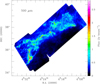 |
Fig. 1 California molecular cloud map at the Herschel 500 μm band. This map is shown from 0 to 20% of the peak value (14.3 Jy beam−1). The 500 μm beam is 36.3′′. The area is about 18 deg2. LkH α101 is a B star, which is the brightest star in the CMC. It is located in the lower left corner and illuminates the surrounding gas. We mark this star with a black cross on the map. |
3 Results
3.1 Herschel H2 column density results
3.1.1 Herschel high-resolution H2 column density map
We applied the getsources tool to derive the column density map of the CMC. Getsources (Men’shchikov et al. 2010, 2012; Men’shchikov 2013) is a multi-scale, multi-wavelength source extraction algorithm. The bash script hirescoldens in getsources was used to create the high-resolution H 2 column density maps (18.2′′) with Herschel four-band emission from 160 to 500 μm. The Hirescoldens methods are described in Appendix A of Palmeirim et al. (2013). The zero-level offsets in the Herschel images are estimated from the Planck and IRAS space telescope (Bernard et al. 2010). In simple words, this method uses a thin graybody model to fit the spectral energy distributions (SEDs) on a pixel-by-pixel basis,
 (1)
(1)
where Iv is the surface brightness at frequency ν, Td is dust temperature at each map pixel, Bν(Td) is the Planck blackbody function, and we assumed a dust opacity law  cm 2 g −1 with β = 2 (Hildebrand 1983; Palmeirim et al. 2013), and Σ is the surface density distribution.
3.1.2 Core extraction from the H2 column density map
We took two steps to extract dense cores from the column density map. First, in order to let the cores stand out, we removed the large-scale diffuse structure in the molecular cloud with cupid findback (Berry et al. 2007). The noise level is 5 × 1020 cm−2, which was determined from off-sources regions in the H2 column density map. We set the smoothing scale to 95′′ judged by visual inspection. Second, we extracted cores from the column density map using the fellwalker algorithm developed by Berry (2015). This algorithm considers all pixels with a value above the noise level. It identifies cores by following the steepest gradient route from each pixel in the map until a significant peak is reached. Each such peak is associated with a single core, and all pixels along routes that end at the same peak are assigned to the associated core. Thus, cores extracted by fellwalker are irregular in shape. However, fellwalker can produce an elliptical approximation to the core shape, centered on the peak value in the core. It does this by first searching for the azimuthal angle that gives the largest marginal profile. With this marginal profile as the major axis, the minor axis is then assumed to be perpendicular to the major axis. The length of each marginal profile is the weighted mean of the distances from the peak to each pixel along the profile, weighted by the pixel data values. A scaling factor is then applied that results in the marginal profile length being equal to the FWHM of the equivalent Gaussian. In other words, for a truly Gaussian core, the final major and minor axes of the elliptical fit would be equal to the FWHM of the Gaussian. Finally, we identified 300 cores in the CMC, which are shown in Fig. 3. The detailed fellwalker setup is listed in Table 2.
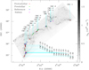 |
Fig. 2 Thirty positions for the IRAM 30m single-pointing observations on the Herschel H 2 column density map. This map is shown from 0 to 20% of the peak value (8.4 × 1022 cm−2). The 500 μm beam is 36.3′′. The 30 observation positions are along the main filament in the CMC. The 14 protostellar cores are plotted with red solid circles, the seven prestellar cores are plotted with green solid circles, the eight observation positions are reference positions that are offset from the cores plotted with blue solid circles, and one position is projected on galaxy 3C111, plotted withpink solid circle. |
3.1.3 Physical parameters in the identified cores
The mass of the core is given by the integral of the column density across the core:
 (2)
(2)
where  is the molecular weight per hydrogen molecule. mH is the H atom mass. A is the area of the core.
Lmaj is the major axis of the ellipse, Lmin is the minor axis. They are equal to the FWHMs of the equivalent Gaussian core. The effective deconvolved radii of the cores were calculated as
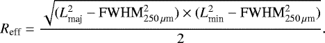 (3)
(3)
The volume (V) of the core is (4∕3)πR3 on the assumption that it is spherical. Then the number density of hydrogen molecule n(H2) in the core is  . The derived masses of the cores are in the range of 0.1−32.9 M⊙, with an average value of 1.9 M⊙. The radii of the cores are in the range of 0.01−0.1 pc, with an average value of 0.04 pc. The number densities are in the range of 1 × 10⁴−1.5 × 106 cm−3, with an average value of 1 × 105 cm−3. The dust temperatures and the H2 number densities are estimated by averaging the values within the fitting ellipse shape. The dust temperatures of the cores are in the range of 12−34 K, with an average value of 15 K. The core parameters are summarized in Table 3.
IRAM 30m observed positions.
3.1.4 Classification of the dense cores
Based on the presence or absence of young stellar objects (YSOs) detected in the infrared data, Enoch et al. (2009) and Dunham et al. (2016) classified the cores into protostellar or starless cores. Harvey et al. (2013) and Broekhoven-Fiene et al. (2014) have indentified two YSO catalogs in the CMC, respectively. In order to resolve the disagreement between these two studies, Lada et al. (2017) reexamined the YSO classifications with the method employed in Lewis & Lada (2016). The YSO distribution in the CMC is shown in Fig. 4. According to the classification and the new YSO catalog in Lada et al. (2017), we found 33 protostellar cores, accounting for 11% of the total cores. In addition, the prestellar cores are the self-gravitating starless cores. The critical Bonnor-Ebert (BE) mass can be used to substitute the virial mass (Ebert 1955; Bonnor 1956; Könyves et al. 2010). The critical BE mass can be calculated as
 (4)
(4)
where RBE is the BE radius, determined by the effective radii of the cores, μp is the mean molecular weight per free particle. Assuming an abundance ratio N(H)/N(He) = 10, μp = 2.33 (Kauffmann et al. 2008). Following Könyves et al. (2010), the assumption of ambient cloud temperature (T = 10 K) is adopted. G is the gravitational constant. kB is the Boltzmann constant. We identified 137 prestellar cores, accounting for about 51% of the starless cores.
3.1.5 Core mass function and core formation efficiency
Salpeter (1955) initially proposed a power-law IMF:
 (5)
(5)
where dN⋆ is the number of stars in the mass range dlogM⋆ and α = 1.35. Chabrier (2003) postulated a log-normal IMF to replace the spliced power laws,
![Mathematical equation: \begin{equation*} \begin{matrix} \hspace*{-10pt}& \frac{\textrm{d}N_{\bigstar }}{\textrm{d}\textrm{log}M_{\bigstar }}\propto \left [ -\frac{(\textrm{log}M_{\bigstar }-\textrm{log}\mu)^{2})}{2\sigma ^{2}} \right ], M_{\bigstar }\leq {1\ M_{\odot}}\\[7pt] \hspace*{-10pt}& \propto M_{\star }^{-1.35}, M_{\bigstar }\geq {1\ M_{\odot}} \end{matrix} ,\end{equation*}](/articles/aa/full_html/2018/12/aa33622-18/aa33622-18-eq10.png) (6)
(6)
where μ = 0.08 and σ =0.67. These parameters changed to μ = 0.25 and σ =0.55 in Chabrier (2005). μ denotes the peak value of the log-normal form IMF in units of M⊙ and σ is the variance in units of log(M⊙).
The core mass function is the mass distribution of the dense cores. In Table 3, the mass of the identified prestellar cores ranges between 0.3 and 13 M⊙. We fit the prestellar CMF with power-law and log-normal forms. Here, we did not take into account the errors in mass estimates, but only statistical uncertrainties:  . The fitting results are shown in Fig. 5. The prestellar cores heavier than 1 M⊙ can be well fit with a power-law function with α = −0.9 ± 0.1, which is shallower than the power-law index of Salpeter (1955). The log-normal fitting result is μ =1.7 ± 0.1 and σ =0.37 ± 0.03. By comparing this with the peak value of the stellar mass of 0.25 M⊙ obtained from the Chabrier (2005) IMF, we suggest that the mass transformation efficiency ϵ in the CMC from the prestellar core to the star is about 15 ± 1%.
In addition, the core formation efficiency (CFE) is the ratio of the total core mass to cloud mass,
 (7)
(7)
We checked the column density map and selected the region without sources to estimate the noise level σ. σ is about 5 × 1020 cm−2. The cloud effective mass is 1.1 × 10⁴ M⊙, which was derived by accounting for emission above the 3σ (see Fig. 4). The total core mass is 600 M⊙. Therefore the CFE is 5.5%.
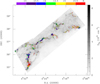 |
Fig. 3 Three hundred cores in the California molecular cloud plotted in the H 2 column density map. This map is shown from 0 to 10% of the peak value (8.4 × 1022 cm−2). The cores are displayed with the measured dust temperature in units of K, coded as shown in the color bar on the top. The major and minor axes of the core ellipse shape in this map are 4 FWHMs of the equivalent Gaussian. |
FELLWALKER configuration parameter values.
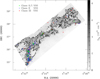 |
Fig. 4 Distribution of YSOs in the Herschel H2 column density map. This map is shown from 0 to 10% of the peak value (8.4 × 1022 cm−2). The noise σ is 0.5 × 1021cm−2 estimated in the region from off-sources. The black contour is 3σ. |
3.2 Molecular-line observations
3.2.1 30 single pointings
The molecular transitions near 90 GHz have typical critical densities (≿ 105 cm−3) for collisional excitation, which makes them excellent tracers for probing dense and cold cores (Foster et al. 2011). Based on the IRAM 30m telescope, 30 positions were observed along the main filament in the CMC. The properties of molecular lines at the 30 positions are summarized in Table 4. We found that 14 positions are protostellar cores, 7 positions are prestellar cores, 8 positions are reference positions that are offset from cores, and 1 position is projected on galaxy 3C111.
Figure A.1 shows H13CO+(1−0), HN 13C(1−0), C 2 H(1−0), HCN(1−0), HCO+(1−0), HNC(1−0), N 2 H+(1−0), C 18 O(1−0), and 13 CO(1−0) spectra. We detected 13 CO(1−0) at all the observed positions, but C 18 O(1−0) only at 27 positions. Generally, the C 18 O(1−0) emission is optically thin, therefore we used C18O(1−0) to determine the local standard of rest velocity (V LSR). For the remaining three position without C18O(1−0) detections, we used 13CO(1−0) to determine the V LSR. The V LSR ranges from −3.63 to 0.52 km s−1. The systemic velocities, line widths, peak intensities, and velocity-integrated intensities were obtained by fitting Gaussian profiles. The obtained parameters of molecular lines at the 30 observed positions are given in Table 4. The detection rates of each molecular line in the 14 protostellar cores, 7 prestellar cores, and the other reference positions are shown in Fig. 6. We also give the detection rates of each molecular line in Table 5. The detection rates of C 2 H(1−0), HCN(1−0), HCO+(1−0), and HNC(1−0) in protostellar cores are higher than that in prestellar cores. Other molecular lines are roughly the same. We also found that the detection rates of the H13CO+(1−0), HN 13C(1−0), and N 2 H+(1−0) in protostellar and prestellar cores are higher than that in the reference positions.
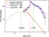 |
Fig. 5 Prestellar CMF fit by power law and log-normal distribution. The error bars correspond to |

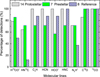 |
Fig. 6 Detection rates of the observed molecular lines (J = 1−0) toward 14 protostellar cores, 7 prestellar cores, and eight observation positions are reference positions that are offset from cores. |
3.2.2 Column density and abundance
We used the ratio with the main isotopologue to determine the optical depths for isotopologue pairs H 13 CO+ and HCO+, and HN 13C and HNC. Assuming that the lineexcitation is at local thermodynamical equilibrium (LTE), the radiative transfer equation that involves the measured brightness temperature(Tr) is given by
![Mathematical equation: \begin{equation*}T_{\textrm{r}}=[J(T_{\textrm{ex}})-J(T_{\textrm{bg}})]\times [1-\exp(-\tau)]f .\end{equation*}](/articles/aa/full_html/2018/12/aa33622-18/aa33622-18-eq13.png) (8)
(8)
Tmb is the corrected main-beam temperature. We have Tr = Tmb. f is the beam filling factor.  . Tbg is the background temperature of the Universe (2.7 K), while Tex is the excitation temperature of the molecular line. τ is the optical depth. For the molecular isotopogue pair, H13CO+ and HCO+, we assumed that the former is optically thin, but the latter is optically thick. We also assumed that they have the same excitation temperature and beam filling factor.
The optical depths of H13CO+ and HCO+ were obtained by comparing the measured brightness temperatures:
 (9)
(9)
Furthermore,
![Mathematical equation: \begin{equation*} \frac{\tau _{12}}{\tau _{13}}=\frac{[^{12}\textrm{C}]}{[^{13}\textrm{C}]} .\end{equation*}](/articles/aa/full_html/2018/12/aa33622-18/aa33622-18-eq16.png) (10)
(10)
The isotopic abundance ratio of ![Mathematical equation: $[^{12}\textrm{C}/{}^{13}\textrm{C}]$](/articles/aa/full_html/2018/12/aa33622-18/aa33622-18-eq17.png) is in the range of 20−70 (Savage et al. 2002). This value is about 20 in the Galactic center, 53 ± 4 in the 4 kpc molecular ring, and 69 ± 6 in the local interstellar medium (ISM; Wilson 1999). This value in our solar system is 89 (Lang 1980). Following Sanhueza et al. (2012), we assumed a constant abundance ratio of 50 for [HCO+∕H13CO+] in the CMC. We obtained the optical depths of HN13C and HNC with the same approach.
is in the range of 20−70 (Savage et al. 2002). This value is about 20 in the Galactic center, 53 ± 4 in the 4 kpc molecular ring, and 69 ± 6 in the local interstellar medium (ISM; Wilson 1999). This value in our solar system is 89 (Lang 1980). Following Sanhueza et al. (2012), we assumed a constant abundance ratio of 50 for [HCO+∕H13CO+] in the CMC. We obtained the optical depths of HN13C and HNC with the same approach.
HCN(1−0), N 2 H+(1−0), and C 2 H(1−0) have a hyperfine structure. We calculated the optical depths of these moleuclar lines with the HyperFine Structure (HFS) method in the CLASS software. The nuclear spin of the nitrogen nucleus leads to the HCN(1−0) rotational transitions showing three components (Loughnane et al. 2012). The optical depth for its main component J F = (12 − 01) was calculated. N2H+(1−0) shows seven components (Keto & Rybicki 2010). Because closely spaced components overlapped, we observed three clusters of lines for N 2 H+(1−0). Two of three lines have three components. Only J F1F = (101−012) is separated from other components, through which we estimated the optical depth of this component. C 2 H(1−0) shows six hyperfine components (Padovani et al. 2009). We estimate the optical depth of the main component as JF = (3∕2, 2 − 1∕2, 1).
Under the assumption of LTE, the column densities at 30 observation positions were estimated via (Mangum & Shirley 2015)
![Mathematical equation: \begin{eqnarray*} N_{\textrm{tot}} &=& \left(\frac{3h}{8 \pi^3 S \mu^2 R_{\textrm{i}}}\right)\left(\frac{Q_{\textrm{rot}}}{g_{\textrm{J}} g_{\textrm{K}} g_{\textrm{I}}}\right) \frac{\exp\left(\frac{E_{\textrm{u}}}{k_{\textrm{B}}T_{\textrm{ex}}}\right)}{\exp\left(\frac{h\nu}{k_{\textrm{B}}T_{\textrm{ex}}}\right) - 1}\\[5pt] &&\quad \times\frac{1}{f\left(J_{\nu}(T_{\textrm{ex}}) - J_{\nu}(T_{\textrm{bg}})\right)}\frac{{\tau_{\nu}} }{1-\exp(-\tau_{\nu})}\int T_{\textrm{mb}} {\textrm{d}}\upsilon,\end{eqnarray*}](/articles/aa/full_html/2018/12/aa33622-18/aa33622-18-eq18.png) (11)
(11)
where h is the Planck constant. S is the line strength. μ is the permanent dipole moment along the axis of symmetry of the molecule4. Ri is the relative intensity normalized to 1. Qrot is the rotational partition function. Eu is the upper energy. gJ is the rotational degeneracy, gK is the K degeneracy, and gI is the nuclear spin degeneracy. We assume that f = 1. For the J → = 1−0 transition of linear molecules
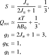 (12)
(12)
where Ju is the upper energy level quantum number. For J = 1–0, Ju = 1. B0 is the rigid rotor rotation constant. At high densities of cores (>105 cm−3), the gas-dust will start to closely couple via collisions (see, e.g., Goldsmith & Langer 1978; Burke & Hollenbach 1983; Goldsmith 2001; Bergin & Tafalla 2007), so we adopted Tex as Td.
In contrast, for non-LTE-based calculations of N(X), multiple transitions of a species X are required, which we do not have. We have observed the CO isotopologues HCO+, HNC, HCN, C2H, and N2H+ in their ground rotational (1–0) transition. We examined the validity of the LTE assumption and applied this assumption to the column density calculation. Usually, in cold sources this occurs when the gas density is higher than the so-called critical density by a factor of 10 or more (Pavlyuchenkov et al. 2008). The critical density is the gas density that is required to start to populate the upper energy level and to excite the line. These densities have been computed for various molecules ina number of papers, see, for example, Shirley (2015). While for the CO (1–0) line the critical density is ~ 103 cm−3, at low T of ~ 10 K. In contrast, the critical densities arehigher for HCO+(1−0), HCN(1−0), HNC(1−0), and N 2 H+(1−0), ≳ 105 cm−3. This implies that at ~10 K, these (1–0) lines could be subthermally excited, and our column density estimates are underestimated by a factor of several.
Under the optically thin assumption, the column densities of 13 CO and C 18 O are calculated. The average optical depths are shown in Fig. 7. The calculation parameters are listed in Table 6. The molecular abundances can be defined as Ntot∕N(H), where N(H) = 2 × N(H2). The statistics of molecular abundances toward 14 protostellar cores and 7 prestellar cores are given in Table 7.
Detection rates of the observed molecular lines (J = 1−0) for 14 protostellar cores, 7 prestellar cores, and 8 observation reference positions that are offset from the cores.
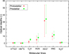 |
Fig. 7 Average optical depths (τ) of the observed molecular lines (J = 1−0). The protostellar cores are plotted with red stars and prestellar cores are shown with green squares. The dashed line shows τ = 1. |
Parameters used to calculate the molecular column densities.
3.2.3 Virial masses
We estimated virial mass from the formula below (MacLaren et al. 1988; Bertoldi & McKee 1992),
 (13)
(13)
where k depends on the core density distribution. Following Parikka et al. (2015), we adopted k = 1.333, which corresponds to a sphere with a power-law density profile ρ ∝ r−1.5. Here, C 18 O(1−0) was used to calulate the virial mass. The velocity dispersion σ is given by
 (14)
(14)
where Tkin is the kinetic temperature. We adopted the dust temperature of core as its kinetic temperature. μtracer is the mass of the observed molecule. ΔV obs is the observed line width. The observed line width consists of thermal and nonthermal components.  is the thermal component of the observed molecular line, while
  is the nonthermal component. The C18O(1−0) virial masses of our cores are in the range of 1.4–5.4 M⊙, with an average value of 3.2 M⊙, which is lower than the average mass of the corresponding cores obtained from the Herschel column density map.
The virial parameter can be given by αvir = Mvir∕M, where M is the mass of the core. When we neglect the contributions of the magnetic field and surface terms in the virial equation, it is considered that cores are gravitationally bound whenever αvir < 1 (e.g., Bertoldi & McKee 1992; Dib et al. 2007b). The virial parameter αvir versus the masses of the cores are displayed in Fig. 8. For two prestellar cores, we found that the values of αvir are close to unity, which may indicate that these cores are in a state of near equipartition between gravity and thermal+turbulent support. For the C18O(1−0) line, 10 out of 12 of the protostellar cores are gravitationally bound according to their αvir values, and 7 prestellar cores display a similar behavior. This is in agreement with the analysis based on estimates of their BE masses.
Statistics of abundance ratios of 14 protostellar and 7 prestellar cores.
 |
Fig. 8 C18O virial parameter αvir vs. core masses for 12 protostellar cores (2 of 14 protostellar cores do not detect C 18 O) and seven prestellar cores. |
3.2.4 Chemical age
We performed a numerical modeling of chemical evolution under the physical conditions typical for a core in the early phase of its evolution. We constructed a model of a “typical core” using the information on the physical condition from Table 3. These are the physical conditions for a “typical core”: a gas density of 1 × 105 cm−3, Tgas = Tdust = 15 K, and a visual extinction Av = 10. The cosmic ray ionization rate and the elemental abundances in the CMC are unclear, therefore we took a typical value of 1.3 × 10⁻¹⁷ s−1 for the ionization rate, and the typical “low metal” abundances (EA1 in Wakelam & Herbst 2008) were used as the initial chemical composition. We used a 0D numerical gas-grain chemical model, that is, a model without anyassumptions about the spatial distribution of the species (Vasyunin et al. 2009, 2017; Vasyunin & Herbst 2013). This chemical model is based on Vasyunin et al. (2017). It employs rate-equation-based three-phase treatment of gas-grain chemistry (gas-ice surface – icy bulk) and the chemical network initially published in Semenov et al. (2010) and then further modified in Vasyunin & Herbst (2013) and Vasyunin et al. (2017). In contrast to Vasyunin et al. (2017), who used a1D model that consisted of 128 0D models and allowed us to calculate 1D distributions of molecules versus radius in the well-studied core L1544, we here calculated just one representative 0D point, because we currently lack knowledge of the inner structure of the cores in CMC to basically calculate the chemical evolution of a unit volume of gas-dust mixture under the provided physical conditions. The chemical age is the evolutionary time when the modeled abundances of the species match the observed values best. We used the modeling results to estimate the chemical age of observed cores. The best-fit criterion is described in Vasyunin et al. (2017; Eq. (17)). The modeling results are shown in Fig. 9. There, we show the fractional abundances of species versus time. The best agreement between the model and observations is attained at ~ 5 × 10⁴ yr.
4 Discussion
4.1 Star formation scenario
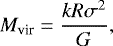
From the Herschel high-resolution H2 column density map, we identified 300 cores in the CMC. According to Kauffmann et al. (2010), if the mass of the core is greater than  , where R is the effective radius of the core, then they have the potential of forming massive stars.[23.7pc] Figure 10 presents a mass versus radius plot of the identified cores in the CMC. We found that three cores, [23.7pc] CMCHerschel-121, CMCHerschel-276, and CMCHerschel-290, lie above the threshold, indicating that they are dense and massive enough to potentially form massive stars. The mass of CMCHerschel-121 is about 33 M⊙, while its effective radius is about 0.08 pc. In our IRAM 30m observations, it is called CMC-9. From Fig. A.1, we found that there is a self-absorption dip in the optically thick line HNC(1−0) of this core, and a blue-skewed profile for HCN(1−0) and HCO+(1−0). We therefore suggest that this core is a collapsing high-mass core candidate. The mass of CMCHerschel-276 is about 4.9 M⊙; we did not observe it with the IRAM 30m telescope. CMCHerschel-290 is called CMC-29 in our IRAM 30m observations. The mass is about 12 M⊙ and the radius is about 0.03 pc. There are no blue or red profiles in its molecular lines. It is relatively quiet.
Figure 11 shows part of the filament that contains the high-mass core (CMCHerschel-121). The local noise level σ is 1.3 × 1021cm−2 in the Herschel H2 column density map. We estimate the filament mass to be above 3σ. The mass of this filament is about 291.9 M⊙, while the length is 6.6 pc. The linear mass is about 44.2 M⊙ pc−1. The critical linear mass density for the turbulent pressure to dominate the thermal pressure can be estimated by  (Jackson et al. 2010). Our IRAM 30m observations include three positions in this filament: CMC-7, CMC-8, and CMC-9. The average C 18 O(1−0) FWHM is 0.84 km s−1. The critical line mass from the C18O(1−0) width is 59.3 M⊙ pc−1, suggesting that the turbulent pressure can support the filament against gravitational collapse.
Turbulence plays an important role in star formation processes (Klessen 2001; Ballesteros-Paredes et al. 2007; Dib et al. 2007b; Liu et al. 2012; Federrath & Klessen 2012; Padoan et al. 2017). The CMF fit from numerical models of turbulent fragmentation in the molecular clouds is more similar to a log-normal form than a power-law form (e.g., Dib & Burkert 2005; Ballesteros-Paredes et al. 2006; Dib et al. 2008; Bailey & Basu 2013; Gong & Ostriker 2015, but see also Padoan & Nordlund 2011; Hennebelle 2018). We find that the CMF of prestellar cores in the CMC is well fit by a log-normal distribution, suggesting that turbulence takes an important role in shaping the CMF.
Based on the offset between the CMF of the Pipe nebula cloud and the IMF of the Trapezium, Alves et al. (2007) proposed that the core-to-star efficiency, ϵ is about 30 ± 10%. However, they did not take into account that some of the cores in their sample may not be prestellar in nature. Because of the low resolution of the Bolocam 1.1 mm, Enoch et al. (2008) only give a lower limit on ϵ 25% for Perseus, Serpens, and Ophiuchus. The prestellar ϵ is about 40% in Aquila (André et al. 2010; Könyves et al. 2015). Nutter & Ward-Thompson (2007) found a turnover at 1.3 M⊙ for SCUBA 850 μm starless cores in Orion. Compared with the turnover at 0.1 M⊙ for a Kroupa (2002) IMF, the starless ϵ in Orion is about 8%. Compared with the turnover at 0.25 M⊙ for a Chabrier (2005) IMF, the starless ϵ in Orion is about 19%. The prestellar ϵ of about 15 ± 1% in the CMCis lower than that in other molecular clouds. The turnover mass of the prestellar CMF in the CMC is ~ 1.7 M⊙. This value is close to the critical BE mass (1.82 M⊙) for a densityof 104 cm−3 and a gas temperature of 10 K (Lada et al. 2008). It is also close to that (~ 2 − 3M⊙), which is an indication that thermal fragmentation may be responsible for the CMF in the Pipe nebula (Lada et al. 2008). We note that like the CMC, the Pipe nebula is a cloud with relatively low star formation for its mass and size.
The CFE is about 5.5% in the CMC, which matches the values of 4.9 and 5.5% in the interarm and spiral-arm regions of the Galactic plane from  to
to  with
with  (Eden et al. 2013). The CFEs for the large-scale structures in our Galaxy are markedly similar in range, but this value is greatly affected by the local environment. The CFE for W3 GMC is 5–13% in the diffuse region, while it is 26–37% in the compressed region as a result of the expansion of W 4 H II region. The feedback from the H II regions also leads to a higher CFE and thus enhanced star formation efficiency (Liu et al. 2015, 2017; Xu et al. 2018). The star formation efficiency (SFE) is the fraction of cloud mass that is converted into stars. Combining the ϵ and CFE in the CMC, we suggest that the SFE is about 1% in the CMC. The typical value in the Milky Way is about 2% (Evans 1991).
The best-fit chemical age of ~5 × 10⁴ yr is well consistent with the hypothesis the CMC is in an early state of evolution, which is somewhat younger than the chemical age for the prototypical prestellar core L1544 (1.6 × 10⁵ yr, see, e.g., Jiménez-Serra et al. 2016; Vasyunin et al. 2017), but there is a difference of one order of magnitude with L134N and TMC-1 (6 × 10⁵ yr, Charnley et al. 2001), and the value is a factor of ~20 lower than the estimated lifetime of the prestellar cores in Aquila (1.2 × 10⁶ yr; Könyves et al. 2015). Obviously, determining the chemical age with a single-point 0D model is merely a rough estimation, as is the concept of the “chemical age” itself. The zero-point in terms of the physical conditions that enter the determination of the chemical age is usually ill defined, and thus, a chemical age is prone to being affected by uncertainty. In addition to this, uncertainties in astrochemical models also limit the accuracy of modeled abundances of species to a factor of a few at best for simple species (Vasyunin et al. 2004, 2008; Wakelam et al. 2005, 2006, 2010). As such, a precise estimation of the chemical age is not physically meaningful. Nevertheless, an order-of-magnitude estimation of this value can be a useful tool to confirm the evolutionary status of protostellar objects (Stahler 1984; Williams 1993; Doty et al. 2002; Brünken et al. 2014).
It is also interesting to estimate how stable the best-fit chemical age is to variations in the model parameters, since our definition of a “typical core” as an average of the core parameters from Table 3 may be considered as somewhat too vague and general. We ran a set of models in which the temperatures of gas and dust were varied by ± 5 K and the gas density was varied by a factor of 2. We found that variations of gas and dust temperature in the range [10−20] K shift the best-fit chemical age in the range [4.0−5.5] × 104 yr, while variations in gas density by a factor of 2 vary the chemical age in the range [3.0−7.3] × 104 yr. We can therefore conclude that the chemical age is not a precise value, since it depends on uncertain parameters. However, an order-of-magnitude estimation of the chemical age is useful because this value in the CMC, which is lower than that in well-studied cores in other clouds, implies that the cores in the CMC are indeed young and the CMC is in a very eary evolutionarystage.
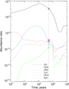 |
Fig. 9 Core chemical age. The colored diamonds indicate the average values of the observations from Table 7. The CO abundance is obtained from 13 CO by [CO]/[13CO] = 50. The best agreement between the model and the median values of the observations is attained at ~ 5 × 10⁴ yr. |
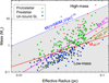 |
Fig. 10 Mass-radius relationship of cores. The red star, green circle, and blue square indicate protostellar, prestellar, and unbound starless cores, respectively. The pink line shows that the mass-radius relationship for all the cores can be well fit with a power law: M ∝ R1.85. The gray shaded region indicates that high-mass stars cannot form (Kauffmann et al. 2010). The green line presents surface densities of 116 M⊙ pc2. The red linepresents the surface density of the critical Bonnor-Ebert sphere. |
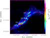 |
Fig. 11 Filament existing high-mass core. σ = 1.3 × 1021cm−2 is the noise estimated in the local region from off-sources. The white contour is 3σ. The pink contour is the average surface density threshold for efficient star formation, 116 M⊙ pc−2 (Lada et al. 2010), corresponding to 7.3 × 1021 cm−2. The green ellipses are cores. The high-mass cores are plotted with pink ellipses. The white solid circle is the IRAM 30m observation point. The red curve is the skeleton of the filament extracted by getfilaments (Men’shchikov 2013). The black squareis a class II YSO. The black triangle is a class 0/I YSO. The five-pointed star is a class III YSO. |
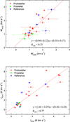 |
Fig. 12 Line widths and velocity-integrated intensities of HCN and HCO+. They follow strong linear relationships, which indicate that HCN and HCO+ couple well and there are tight chemical connections. The 14 protostellar cores are plotted with red stars, the seven prestellar cores are plotted with green boxes, and the eight observation positions are reference positions that are offset from the cores. They are plotted with blue inverted triangles. |
4.2 Dynamics
The line widths extracted from single-point observation hold important information on the core kinematics. The average widths of 13 CO(1−0) and C 18 O(1−0) are 1.6 and 0.92 km s−1 in the CMC, which roughly corresponds to those in the Planck cold dust clumps (1.3 km s−1 for 13 CO and 0.8 km s−1 for C 18 O; Wu et al. 2012) and those with valid detections of HCO+ or HCN (1.67 km s−1 for 13CO and 1.08 km s−1 for C18O) in Yuan et al. (2016). We calculated the asymmetry parameter (Mardones et al. 1997), δV = (V thick − V thin)∕dV thin. The asymmetry parameter has been used to quantify the asymmetry of an optical thick molecular line, where V thick is the peak velocity of an optical thick line. Vthin is the peak velocity of an optical thin line. dVthin is hte full width at half-maximum of the optically thin line. A line is considered to have a blue-skewed profile if δV < −0.25, and it is red-skewed if δV > 0.25. The optically thick line HCO+(1−0) is a good tracer of the motion of infall. Usually, HCO+(1−0) and HNC(1−0) are optically thick, and C18O(1−0) is optically thin. Evidence of infall motion is observable in self-absorbed and optically thick line profiles, which show a combination of a double peak with a brighter blue peak or a skewed single blue peak, or optically thin lines that peak at the self-absorption dip of the optically thick line (He et al. 2015). We find that six cores show a blue-skewed profile and four cores show a red-skewed profile that possibly indicates outflowing motions. The skewed profiles of the molecular line are shown in Table 8.
4.3 Chemical composition
HCN and HCO+ have high permanent dipole moments. They are good tracers of high-density gas (≥ 106 cm−3), therefore, their emissions are well suited to studying the densest regions in a molecular cloud. The line widths of HCN(1−0) and HCO+(1−0) at the observed positions are in the range of 0.66−2.65 km s−1 and 0.66−2.81 km s−1, with an average value of 1.41 and 1.49 km s−1, respectively. The velocity-integrated intensities ofHCN and HCO+ are in the range of 0.28−4.63 and 0.29−8.25 K km s−1, with an average value of 1.66 and 3.04 K km s−1, respectively. We found strong linear correlations between HCN(1−0) and HCO+(1−0) in line widths and velocity-integrated intensities. The line widths are  .
.  is the adjusted R-squared, that is, the fit residuals relative to the error (variance) estimates, which is an important parameter to indicate how well some terms fit a curve or line.
  indicates that about 85% of the data points can be well represented by the fitted line. The velocity-integrated intensities are
  . R2 = 0.77 indicates that about 88% of the data points can be well represented by the fitted line. We show these strong linear relationships between HCN and HCO+ in Fig. 12. The intensities ofHCN and HCO+ in infrared dark clouds show a linear relation,
  (Liu et al. 2013). Yuan et al. (2016) found that the intensities of HCN and HCO+ in Planck cold clumps could be fit by a power-law relation,
  .
.
The tight correlation between the line widths and line intensities of HCN and HCO+ in various CMC cores is due to the two-body nature of the chemical processes by which these species are formed and destroyed, and the lack of strong line excitation gradients in a typical molecular cloud core (Turner 1995; Turner et al. 1997). The denser the core, the more readily both of these molecules form through ion-molecule and neutral-neutral gas-phase reactions. Similarly, the denser the core, the more efficiently HCO+ dissociates in collisions with electrons, while HCN freezes out more efficiently onto dust grains.
The HCN synthesis is driven by a slow neutral–neutral reaction N + CH2 → HCN + H, and later, a chemical quasi steady-state is attained. This equilibrium is governed by a protonation-recombination cycle: HCN + H → HCNH+ +H2, HCNH+ + e− → HCN + H, with a 34% probability5. The HCO+ chemistry begins with the conversion of almost the entire C budget into CO, which can then react with H
 to form HCO+ and H. Later, a chemical steady state is attained for HCO+, with the protonation of CO followed by the dissociative recombination of HCO+ back into H and CO. The direct chemical relationship between HCO+ and HCN through common or closely related reactions is quite limited. Only one chemical reaction in our chemical model may lead to the direct correlation between HCO+ and HCN: HCO+ + HCN → HCNH+ + CO. However, at least in the model considered, this reaction is a destruction channel of moderate importance (up to 15% of total HCN destruction rate at 105 yr, and up to 7% of total HCO+ destruction rate at 104 yr of evolution).
The abundances of the isomer pair HNC and HCN are roughly equal at low temperature (Irvine & Schloerb 1984; Schilke et al. 1992; Ungerechts et al. 1997; Graninger et al. 2014). The average observed abundances of HNC and HCN are roughly equal in the CMC. The value of~10−9 for the HNCand HCN abundance also match previous works well (Hirota et al. 1998; Padovani et al. 2011). We found that the average abundance ratio of HCN/HNC in protostellar cores does not have a clear difference with that in prestellar cores.
A combination of the CO optically thin isotopologue and N2 H+, for example, can be employed to estimate the degree of the CO freeze-out, which can also be used as a coarse indicator of the core age and the onset of the star formation process. The main reaction that effectively removes N2 H+ from the gas when CO is still present is N2 H+ + CO → HCO+ + N2. Later, after ~ 105−106 yr, when substantial CO freeze-out is expected to occur in dense cores, this destruction channel becomes inefficient. The average abundance ratio of HCO+/N2H+ in protostellar cores is about three times higher than that in prestellar cores. We also found that the average abundance ratio of HCO+/HNC in protostellar cores is about twice higher than that in prestellar cores. There are obvious differences for HCO+/HNC and HCO+/N2H+ in the protostellar cores with the prestellar cores. We therefore suggest that HCO+/HNC and HCO+/N2H+ are chemical clocks. Our results are similar to those of previous studies (e.g., Sanhueza et al. 2012; Hoq et al. 2013).
Molecular line skewed profile.
5 Conclusions
We made a high-resolution (18.2′′) H 2 column density map with the Herschel data. Using this map, we extracted a complete core sample with the fellwalker algorithm. In order to estimate the chemical composition and evolution of the cores in the CMC, we used the IRAM 30m telescope to carry out new single-point molecular line observations near 90 GHz along the CMC main filament. These molecular lines include 13 CO(1−0), C 18 O(1−0), N 2 H+(1−0), HNC(1−0), HCO+(1−0), HCN(1−0), C2H(1−0), HN 13C(1−0), and H 13 CO+(1−0). The main results are summarized as follows:
- (1)
We extracted 300 cores from the high-resolution H2 column density map. These identified cores contain 33 protostellar cores, 137 prestellar cores, and 130 unbound starless cores. The number of the prestellar cores accounts for about 51% of the starless cores.
- (2)
The core masses are in the range of 0.12−33 M⊙ with an average value of 1.9 M⊙, while theradii are in the range of 0.01−0.1 pc with an average value of 0.04 pc. Three cores can evolve into high-mass stars. The mass of the high-mass core CMCHerschel-121 is 33 M⊙, while its radius is 0.08 pc. Moreover, this core, located at a filament, shows an infall feature, suggesting that this core may be in a state of collapse.
- (3)
The prestellar core CMF is slightly steeper than the Galactic field IMF. The prestellar core CMF can be fit by a lognormal distribution with a peak value μ = 1.7 M⊙ and σ = 0.37 ± 0.03. When fit by a power law in the high-mass end, the exponent of the power law is − 0.9 ± 0.1. It should be noted, however, that the CMC is very young, and thus, its population of dense cores is likely to still have ongoing accretion, which will tend to modify or flatten the CMF (Dib et al. 2010). Based on the position of the peak of the CMF with respect to the value of the peak in the (Chabrier 2005) IMF, we propose that the core-to-star efficiency, ϵ, at this stage of its evolution is 15 ± 1%. With a CFE of ≈5.5%, this translates into an SFE of ≈1%.
- (4)
Based on the IRAM 30m telescope single-pointing observations at 30 positions, we find that six cores show a blue-skewed profile and four cores show a red-skewed profile.
- (5)
The line widths and line intensities of HCN correlate well with those of HCO+. [HCO+]/[HNC] and [HCO+]/[N2H+] in protostellar cores are obviously higher than those in pretellar cores, which can be used as chemical clocks.
- (6)
The best-fit chemical age of the cold cores is about 5 × 10⁴ yr, which we derived by fitting the data with an elaborate chemical model.
Acknowledgements
We acknowledge valuable comments from the referee. We thank Charles J. Lada for useful discussion on the manuscript. We thank A. Men’shchikov, D. S. Berry, and S. Bardeau for their technical support with Getsources, Starlink and Gildas, respectively. This work is supported by National Key R&D Program of China (No. 2017YFA0402600; 2017YFA0402702), National Key Basic Research Program of China (973 Program) (No. 2015CB857101), National Natural Science foundation of China (No. 11703040; 11703074; 11721303; 11763002; U1431111), and Chinese Government Scholarship (No. 201804910583). D.A.S. acknowledges support from the Heidelberg Institute of Theoretical Studies for the project “Chemical kinetics models and visualization tools: Bridging biology and astronomy”. A.I.V. acknowledges support by the Russian Science Foundation (No. 18-12-00351). K.W. acknowledges support by the German Research Foundation (grant WA3628-1/1).
Appendix A Additional figure
 |
Fig. A.1 Thirty molecular lines of the IRAM 30m observation point. The green curves indicate the Gauss-fit profile. The red dashed lines mark the position of the local standard of rest velocity. The blue lines mark the position of the N 2 H + (1−0) and HCN(1−0) hyperfine structure. |
 |
Fig. A.1 continued. |
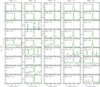 |
Fig. A.1 continued. |
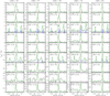 |
Fig. A.1 continued. |
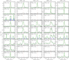 |
Fig. A.1 continued. |
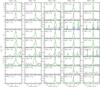 |
Fig. A.1 continued. |
References
- Alves, J., Lombardi, M., & Lada, C. J. 2007, A&A, 462, L17 [NASA ADS] [CrossRef] [EDP Sciences] [Google Scholar]
- André, P., Men’shchikov, A., Bontemps, S., et al. 2010, A&A, 518, L102 [NASA ADS] [CrossRef] [EDP Sciences] [Google Scholar]
- André, P., Di Francesco, J., Ward-Thompson, D., et al. 2014, Protostars and Planets VI (Tucson, AZ: University of Arizona Press), 27 [Google Scholar]
- Bailey, N. D., & Basu, S. 2013, ApJ, 766, 27 [NASA ADS] [CrossRef] [Google Scholar]
- Ballesteros-Paredes, J., Gazol, A., Kim, J., et al. 2006, ApJ, 637, 384 [NASA ADS] [CrossRef] [Google Scholar]
- Ballesteros-Paredes, J., Klessen, R. S., Mac Low, M.-M., & Vazquez-Semadeni, E. 2007, Protostars and Planets V (Tucson, AZ: University of Arizona Press), 63 [Google Scholar]
- Barsony, M., Schombert, J. M., & Kis-Halas, K. 1991, ApJ, 379, 221 [NASA ADS] [CrossRef] [Google Scholar]
- Bergin, E. A., & Tafalla, M. 2007, ARA&A, 45, 339 [NASA ADS] [CrossRef] [Google Scholar]
- Bernard, J.-P., Paradis, D., Marshall, D. J., et al. 2010, A&A, 518, L88 [NASA ADS] [CrossRef] [EDP Sciences] [Google Scholar]
- Berry, D. S. 2015, Astron. Comput., 10, 22 [NASA ADS] [CrossRef] [Google Scholar]
- Berry, D. S., Reinhold, K., Jenness, T., & Economou, F. 2007, in Astronomical Data Analysis Software and Systems XVI, eds. R. A. Shaw, F. Hill, & D. J. Bell, ASP Conf. Ser., 376, 425 [NASA ADS] [Google Scholar]
- Bertoldi, F., & McKee, C. F. 1992, ApJ, 395, 140 [NASA ADS] [CrossRef] [Google Scholar]
- Bonnor, W. B. 1956, MNRAS, 116, 351 [CrossRef] [Google Scholar]
- Broekhoven-Fiene, H., Matthews, B. C., Harvey, P. M., et al. 2014, ApJ, 786, 37 [NASA ADS] [CrossRef] [Google Scholar]
- Broekhoven-Fiene, H., Matthews, B. C., Harvey, P., et al. 2018, ApJ, 852, 73 [NASA ADS] [CrossRef] [Google Scholar]
- Brünken, S., Sipilä, O., Chambers, E. T., et al. 2014, Nature, 516, 219 [NASA ADS] [CrossRef] [PubMed] [Google Scholar]
- Burke, J. R., & Hollenbach, D. J. 1983, ApJ, 265, 223 [NASA ADS] [CrossRef] [Google Scholar]
- Chabrier, G. 2003, ApJ, 586, L133 [NASA ADS] [CrossRef] [Google Scholar]
- Chabrier, G. 2005, in The Initial Mass Function 50 Years Later, eds. E. Corbelli, F. Palla, & H. Zinnecker, Astrophys. Space Sci. Lib., 327, 41 [NASA ADS] [CrossRef] [Google Scholar]
- Charnley, S. B., Rodgers, S. D., & Ehrenfreund, P. 2001, A&A, 378, 1024 [NASA ADS] [CrossRef] [EDP Sciences] [Google Scholar]
- Dahm, S. E. 2008, The Young Cluster and Star Forming Region NGC 2264, ed. B. Reipurth, 966 [Google Scholar]
- Dib, S. 2014, MNRAS, 444, 1957 [NASA ADS] [CrossRef] [MathSciNet] [Google Scholar]
- Dib, S., & Burkert, A. 2005, ApJ, 630, 238 [NASA ADS] [CrossRef] [Google Scholar]
- Dib, S., Kim, J., & Shadmehri, M. 2007a, MNRAS, 381, L40 [NASA ADS] [CrossRef] [Google Scholar]
- Dib, S., Kim, J., Vázquez-Semadeni, E., Burkert, A., & Shadmehri, M. 2007b, ApJ, 661, 262 [NASA ADS] [CrossRef] [Google Scholar]
- Dib, S., Brandenburg, A., Kim, J., Gopinathan, M., & André, P. 2008, ApJ, 678, L105 [NASA ADS] [CrossRef] [Google Scholar]
- Dib, S., Shadmehri, M., Padoan, P., et al. 2010, MNRAS, 405, 401 [NASA ADS] [Google Scholar]
- Dib, S., Schmeja, S., & Hony, S. 2017, MNRAS, 464, 1738 [NASA ADS] [CrossRef] [Google Scholar]
- Doty, S. D., van Dishoeck, E. F., van der Tak, F. F. S., & Boonman, A. M. S. 2002, A&A, 389, 446 [NASA ADS] [CrossRef] [EDP Sciences] [Google Scholar]
- Dunham, M. M., Offner, S. S. R., Pineda, J. E., et al. 2016, ApJ, 823, 160 [NASA ADS] [CrossRef] [Google Scholar]
- Ebert, R. 1955, Z. Astrophys., 37, 217 [NASA ADS] [Google Scholar]
- Eden, D. J., Moore, T. J. T., Morgan, L. K., Thompson, M. A., & Urquhart, J. S. 2013, MNRAS, 431, 1587 [NASA ADS] [CrossRef] [Google Scholar]
- Enoch, M. L., Evans, II, N. J., Sargent, A. I., et al. 2008, ApJ, 684, 1240 [NASA ADS] [CrossRef] [Google Scholar]
- Enoch, M. L., Evans, II, N. J., Sargent, A. I., & Glenn, J. 2009, ApJ, 692, 973 [NASA ADS] [CrossRef] [Google Scholar]
- Evans, II, N. J. 1991, in Frontiers of Stellar Evolution, ed. D. L. Lambert, ASP Conf. Ser., 20, 45 [NASA ADS] [Google Scholar]
- Federrath, C., & Klessen, R. S. 2012, ApJ, 761, 156 [NASA ADS] [CrossRef] [Google Scholar]
- Foster, J. B., Jackson, J. M., Barnes, P. J., et al. 2011, ApJS, 197, 25 [NASA ADS] [CrossRef] [Google Scholar]
- Gerin, M., Fossé, D., & Roueff, E. 2003, in SFChem 2002: Chemistry as a Diagnostic of Star Formation, eds. C. L. Curry & M. Fich, 81 [Google Scholar]
- Goldsmith, P. F. 2001, ApJ, 557, 736 [NASA ADS] [CrossRef] [MathSciNet] [Google Scholar]
- Goldsmith, P. F., & Langer, W. D. 1978, ApJ, 222, 881 [NASA ADS] [CrossRef] [Google Scholar]
- Gong, M., & Ostriker, E. C. 2015, ApJ, 806, 31 [NASA ADS] [CrossRef] [Google Scholar]
- Graninger, D. M., Herbst, E., Öberg, K. I., & Vasyunin, A. I. 2014, ApJ, 787, 74 [NASA ADS] [CrossRef] [Google Scholar]
- Griffin, M. J., Abergel, A., Abreu, A., et al. 2010, A&A, 518, L3 [Google Scholar]
- Harvey, P. M., Fallscheer, C., Ginsburg, A., et al. 2013, ApJ, 764, 133 [NASA ADS] [CrossRef] [Google Scholar]
- He, Y.-X., Zhou, J.-J., Esimbek, J., et al. 2015, MNRAS, 450, 1926 [NASA ADS] [CrossRef] [Google Scholar]
- Hennebelle, P. 2018, A&A, 611, A24 [NASA ADS] [CrossRef] [EDP Sciences] [Google Scholar]
- Hildebrand, R. H. 1983, QJRAS, 24, 267 [NASA ADS] [Google Scholar]
- Hirota, T., Yamamoto, S., Mikami, H., & Ohishi, M. 1998, ApJ, 503, 717 [NASA ADS] [CrossRef] [Google Scholar]
- Hony, S., Gouliermis, D. A., Galliano, F., et al. 2015, MNRAS, 448, 1847 [NASA ADS] [CrossRef] [Google Scholar]
- Hoq, S., Jackson, J. M., Foster, J. B., et al. 2013, ApJ, 777, 157 [NASA ADS] [CrossRef] [Google Scholar]
- Irvine, W. M., & Schloerb, F. P. 1984, ApJ, 282, 516 [Google Scholar]
- Jackson, J. M., Finn, S. C., Chambers, E. T., Rathborne, J. M., & Simon, R. 2010, ApJ, 719, L185 [NASA ADS] [CrossRef] [Google Scholar]
- Jiménez-Serra, I., Vasyunin, A. I., Caselli, P., et al. 2016, ApJ, 830, L6 [Google Scholar]
- Kauffmann, J., Bertoldi, F., Bourke, T. L., Evans, II, N. J., & Lee, C. W. 2008, A&A, 487, 993 [NASA ADS] [CrossRef] [EDP Sciences] [Google Scholar]
- Kauffmann, J., Pillai, T., Shetty, R., Myers, P. C., & Goodman, A. A. 2010, ApJ, 716, 433 [NASA ADS] [CrossRef] [Google Scholar]
- Keto, E., & Rybicki, G. 2010, ApJ, 716, 1315 [NASA ADS] [CrossRef] [Google Scholar]
- Klessen, R. S. 2001, ApJ, 556, 837 [Google Scholar]
- Kong, S., Lada, C. J., Lada, E. A., et al. 2015, ApJ, 805, 58 [NASA ADS] [CrossRef] [Google Scholar]
- Könyves, V., André, P., Men’shchikov, A., et al. 2010, A&A, 518, L106 [NASA ADS] [CrossRef] [EDP Sciences] [Google Scholar]
- Könyves, V., André, P., Men’shchikov, A., et al. 2015, A&A, 584, A91 [NASA ADS] [CrossRef] [EDP Sciences] [Google Scholar]
- Kroupa, P. 2002, Science, 295, 82 [NASA ADS] [CrossRef] [PubMed] [Google Scholar]
- Kutner, M. L., Tucker, K. D., Chin, G., & Thaddeus, P. 1977, ApJ, 215, 521 [NASA ADS] [CrossRef] [Google Scholar]
- Lang, K. R. 1980, Science, 207, 174 [NASA ADS] [CrossRef] [Google Scholar]
- Lada, C. J., Muench, A. A., Rathborne, J., Alves, J. F., & Lombardi, M. 2008, ApJ, 672, 410 [NASA ADS] [CrossRef] [Google Scholar]
- Lada, C. J., Lombardi, M., & Alves, J. F. 2009, ApJ, 703, 52 [NASA ADS] [CrossRef] [Google Scholar]
- Lada, C. J., Lewis, J. A., Lombardi, M., & Alves, J. 2017, A&A, 606, A100 [NASA ADS] [CrossRef] [EDP Sciences] [Google Scholar]
- Lewis, J. A., & Lada, C. J. 2016, ApJ, 825, 91 [NASA ADS] [CrossRef] [Google Scholar]
- Li, D. L., Esimbek, J., Zhou, J. J., et al. 2014, A&A, 567, A10 [NASA ADS] [CrossRef] [EDP Sciences] [Google Scholar]
- Liu, T., Wu, Y., & Zhang, H. 2012, ApJS, 202, 4 [NASA ADS] [CrossRef] [Google Scholar]
- Liu, X.-L., Wang, J.-J., & Xu, J.-L. 2013, MNRAS, 431, 27 [NASA ADS] [CrossRef] [Google Scholar]
- Liu, H.-L., Wu, Y., Li, J., et al. 2015, ApJ, 798, 30 [NASA ADS] [CrossRef] [Google Scholar]
- Liu, T., Lacy, J., Li, P. S., et al. 2017, ApJ, 849, 25 [NASA ADS] [CrossRef] [Google Scholar]
- Loughnane, R. M., Redman, M. P., Thompson, M. A., et al. 2012, MNRAS, 420, 1367 [NASA ADS] [CrossRef] [Google Scholar]
- MacLaren, I., Richardson, K. M., & Wolfendale, A. W. 1988, ApJ, 333, 821 [NASA ADS] [CrossRef] [Google Scholar]
- Mangum, J. G., & Shirley, Y. L. 2015, PASP, 127, 266 [NASA ADS] [CrossRef] [Google Scholar]
- Mardones, D., Myers, P. C., Tafalla, M., et al. 1997, ApJ, 489, 719 [NASA ADS] [CrossRef] [Google Scholar]
- Men’shchikov, A. 2013, A&A, 560, A63 [NASA ADS] [CrossRef] [EDP Sciences] [Google Scholar]
- Men’shchikov, A., André, P., Didelon, P., et al. 2010, A&A, 518, L103 [NASA ADS] [CrossRef] [EDP Sciences] [Google Scholar]
- Men’shchikov, A., André, P., Didelon, P., et al. 2012, A&A, 542, A81 [NASA ADS] [CrossRef] [EDP Sciences] [Google Scholar]
- Motte, F., Nony, T., Louvet, F., et al. 2018, Nat. Astron., 2, 478 [NASA ADS] [CrossRef] [Google Scholar]
- Muench, A. A., Lada, E. A., Lada, C. J., & Alves, J. 2002, ApJ, 573, 366 [NASA ADS] [CrossRef] [Google Scholar]
- Nutter, D., & Ward-Thompson, D. 2007, MNRAS, 374, 1413 [NASA ADS] [CrossRef] [Google Scholar]
- Padoan, P., & Nordlund, Å. 2011, ApJ, 741, L22 [NASA ADS] [CrossRef] [Google Scholar]
- Padoan, P., Haugbølle, T., Nordlund, Å., & Frimann, S. 2017, ApJ, 840, 48 [NASA ADS] [CrossRef] [Google Scholar]
- Padovani, M., Walmsley, C. M., Tafalla, M., Galli, D., & Müller, H. S. P. 2009, A&A, 505, 1199 [NASA ADS] [CrossRef] [EDP Sciences] [Google Scholar]
- Padovani, M., Walmsley, C. M., Tafalla, M., Hily-Blant, P., & Pineau Des Forêts G. 2011, A&A, 534, A77 [NASA ADS] [CrossRef] [EDP Sciences] [Google Scholar]
- Palmeirim, P., André, P., Kirk, J., et al. 2013, A&A, 550, A38 [NASA ADS] [CrossRef] [EDP Sciences] [Google Scholar]
- Parikka, A., Juvela, M., Pelkonen, V.-M., Malinen, J., & Harju, J. 2015, A&A, 577, A69 [NASA ADS] [CrossRef] [EDP Sciences] [Google Scholar]
- Pavlyuchenkov, Y., Wiebe, D., Shustov, B., et al. 2008, ApJ, 689, 335 [NASA ADS] [CrossRef] [Google Scholar]
- Poglitsch, A., Waelkens, C., Geis, N., et al. 2010, A&A, 518, L2 [NASA ADS] [CrossRef] [EDP Sciences] [Google Scholar]
- Rivera-Ingraham, A., Martin, P. G., Polychroni, D., et al. 2013, ApJ, 766, 85 [NASA ADS] [CrossRef] [Google Scholar]
- Salpeter, E. E. 1955, ApJ, 121, 161 [Google Scholar]
- Sanhueza, P., Jackson, J. M., Foster, J. B., et al. 2012, ApJ, 756, 60 [NASA ADS] [CrossRef] [Google Scholar]
- Savage, C., Apponi, A. J., Ziurys, L. M., & Wyckoff, S. 2002, ApJ, 578, 211 [NASA ADS] [CrossRef] [Google Scholar]
- Schilke, P., Walmsley, C. M., Pineau Des Forets, G., et al. 1992, A&A, 256, 595 [Google Scholar]
- Schneider, F. R. N., Sana, H., Evans, C. J., et al. 2018, Science, 361, aat7032 [NASA ADS] [CrossRef] [Google Scholar]
- Semenov, D., Hersant, F., Wakelam, V., et al. 2010, A&A, 522, A42 [NASA ADS] [CrossRef] [EDP Sciences] [Google Scholar]
- Shadmehri, M. 2004, MNRAS, 354, 375 [NASA ADS] [CrossRef] [Google Scholar]
- Shirley, Y. L. 2015, PASP, 127, 299 [NASA ADS] [CrossRef] [Google Scholar]
- Stahler, S. W. 1984, ApJ, 281, 209 [NASA ADS] [CrossRef] [Google Scholar]
- Turner, B. E. 1995, ApJ, 449, 635 [NASA ADS] [CrossRef] [Google Scholar]
- Turner, B. E., Pirogov, L., & Minh, Y. C. 1997, ApJ, 483, 235 [NASA ADS] [CrossRef] [Google Scholar]
- Ungerechts, H., Bergin, E. A., Goldsmith, P. F., et al. 1997, ApJ, 482, 245 [NASA ADS] [CrossRef] [PubMed] [Google Scholar]
- Vasyunin, A. I., & Herbst, E. 2013, ApJ, 762, 86 [NASA ADS] [CrossRef] [Google Scholar]
- Vasyunin, A. I., Sobolev, A. M., Wiebe, D. S., & Semenov, D. A. 2004, Astron. Lett., 30, 566 [NASA ADS] [CrossRef] [Google Scholar]
- Vasyunin, A. I., Semenov, D., Henning, T., et al. 2008, ApJ, 672, 629 [NASA ADS] [CrossRef] [Google Scholar]
- Vasyunin, A. I., Semenov, D. A., Wiebe, D. S., & Henning, T. 2009, ApJ, 691, 1459 [NASA ADS] [CrossRef] [Google Scholar]
- Vasyunin, A. I., Caselli, P., Dulieu, F., & Jiménez-Serra, I. 2017, ApJ, 842, 33 [Google Scholar]
- Wakelam, V., & Herbst, E. 2008, ApJ, 680, 371 [NASA ADS] [CrossRef] [Google Scholar]
- Wakelam, V., Selsis, F., Herbst, E., & Caselli, P. 2005, A&A, 444, 883 [NASA ADS] [CrossRef] [EDP Sciences] [Google Scholar]
- Wakelam, V., Herbst, E., & Selsis, F. 2006, A&A, 451, 551 [NASA ADS] [CrossRef] [EDP Sciences] [Google Scholar]
- Wakelam, V., Herbst, E., Le Bourlot, J., et al. 2010, A&A, 517, A21 [NASA ADS] [CrossRef] [EDP Sciences] [Google Scholar]
- Weisz, D. R., Johnson, L. C., Foreman-Mackey, D., et al. 2015, ApJ, 806, 198 [NASA ADS] [CrossRef] [Google Scholar]
- Williams, D. A. 1993, in Rev. Mod. Astron., ed. G. Klare, 6, 49 [NASA ADS] [Google Scholar]
- Williams, J. P., Blitz, L., & Stark, A. A. 1995, ApJ, 451, 252 [NASA ADS] [CrossRef] [Google Scholar]
- Wilson, T. L. 1999, Rep. Prog. Phys., 62, 143 [Google Scholar]
- Wu, Y., Liu, T., Meng, F., et al. 2012, ApJ, 756, 76 [NASA ADS] [CrossRef] [Google Scholar]
- Xu, J.-L., Xu, Y., Zhang, C.-P., et al. 2018, A&A, 609, A43 [NASA ADS] [CrossRef] [EDP Sciences] [Google Scholar]
- Yuan, J., Wu, Y., Liu, T., et al. 2016, ApJ, 820, 37 [NASA ADS] [CrossRef] [Google Scholar]
All Tables
Detection rates of the observed molecular lines (J = 1−0) for 14 protostellar cores, 7 prestellar cores, and 8 observation reference positions that are offset from the cores.
All Figures
|
Fig. 1 California molecular cloud map at the Herschel 500 μm band. This map is shown from 0 to 20% of the peak value (14.3 Jy beam−1). The 500 μm beam is 36.3′′. The area is about 18 deg2. LkH α101 is a B star, which is the brightest star in the CMC. It is located in the lower left corner and illuminates the surrounding gas. We mark this star with a black cross on the map. |
| In the text | |
|
Fig. 2 Thirty positions for the IRAM 30m single-pointing observations on the Herschel H 2 column density map. This map is shown from 0 to 20% of the peak value (8.4 × 1022 cm−2). The 500 μm beam is 36.3′′. The 30 observation positions are along the main filament in the CMC. The 14 protostellar cores are plotted with red solid circles, the seven prestellar cores are plotted with green solid circles, the eight observation positions are reference positions that are offset from the cores plotted with blue solid circles, and one position is projected on galaxy 3C111, plotted withpink solid circle. |
| In the text | |
|
Fig. 3 Three hundred cores in the California molecular cloud plotted in the H 2 column density map. This map is shown from 0 to 10% of the peak value (8.4 × 1022 cm−2). The cores are displayed with the measured dust temperature in units of K, coded as shown in the color bar on the top. The major and minor axes of the core ellipse shape in this map are 4 FWHMs of the equivalent Gaussian. |
| In the text | |
|
Fig. 4 Distribution of YSOs in the Herschel H2 column density map. This map is shown from 0 to 10% of the peak value (8.4 × 1022 cm−2). The noise σ is 0.5 × 1021cm−2 estimated in the region from off-sources. The black contour is 3σ. |
| In the text | |
|
Fig. 5 Prestellar CMF fit by power law and log-normal distribution. The error bars correspond to |
| In the text | |
|
Fig. 6 Detection rates of the observed molecular lines (J = 1−0) toward 14 protostellar cores, 7 prestellar cores, and eight observation positions are reference positions that are offset from cores. |
| In the text | |
|
Fig. 7 Average optical depths (τ) of the observed molecular lines (J = 1−0). The protostellar cores are plotted with red stars and prestellar cores are shown with green squares. The dashed line shows τ = 1. |
| In the text | |
|
Fig. 8 C18O virial parameter αvir vs. core masses for 12 protostellar cores (2 of 14 protostellar cores do not detect C 18 O) and seven prestellar cores. |
| In the text | |
|
Fig. 9 Core chemical age. The colored diamonds indicate the average values of the observations from Table 7. The CO abundance is obtained from 13 CO by [CO]/[13CO] = 50. The best agreement between the model and the median values of the observations is attained at ~ 5 × 10⁴ yr. |
| In the text | |
|
Fig. 10 Mass-radius relationship of cores. The red star, green circle, and blue square indicate protostellar, prestellar, and unbound starless cores, respectively. The pink line shows that the mass-radius relationship for all the cores can be well fit with a power law: M ∝ R1.85. The gray shaded region indicates that high-mass stars cannot form (Kauffmann et al. 2010). The green line presents surface densities of 116 M⊙ pc2. The red linepresents the surface density of the critical Bonnor-Ebert sphere. |
| In the text | |
|
Fig. 11 Filament existing high-mass core. σ = 1.3 × 1021cm−2 is the noise estimated in the local region from off-sources. The white contour is 3σ. The pink contour is the average surface density threshold for efficient star formation, 116 M⊙ pc−2 (Lada et al. 2010), corresponding to 7.3 × 1021 cm−2. The green ellipses are cores. The high-mass cores are plotted with pink ellipses. The white solid circle is the IRAM 30m observation point. The red curve is the skeleton of the filament extracted by getfilaments (Men’shchikov 2013). The black squareis a class II YSO. The black triangle is a class 0/I YSO. The five-pointed star is a class III YSO. |
| In the text | |
|
Fig. 12 Line widths and velocity-integrated intensities of HCN and HCO+. They follow strong linear relationships, which indicate that HCN and HCO+ couple well and there are tight chemical connections. The 14 protostellar cores are plotted with red stars, the seven prestellar cores are plotted with green boxes, and the eight observation positions are reference positions that are offset from the cores. They are plotted with blue inverted triangles. |
| In the text | |
|
Fig. A.1 Thirty molecular lines of the IRAM 30m observation point. The green curves indicate the Gauss-fit profile. The red dashed lines mark the position of the local standard of rest velocity. The blue lines mark the position of the N 2 H + (1−0) and HCN(1−0) hyperfine structure. |
| In the text | |
|
Fig. A.1 continued. |
| In the text | |
|
Fig. A.1 continued. |
| In the text | |
|
Fig. A.1 continued. |
| In the text | |
|
Fig. A.1 continued. |
| In the text | |
|
Fig. A.1 continued. |
| In the text | |
Current usage metrics show cumulative count of Article Views (full-text article views including HTML views, PDF and ePub downloads, according to the available data) and Abstracts Views on Vision4Press platform.
Data correspond to usage on the plateform after 2015. The current usage metrics is available 48-96 hours after online publication and is updated daily on week days.
Initial download of the metrics may take a while.