| Issue |
A&A
Volume 620, December 2018
|
|
|---|---|---|
| Article Number | A52 | |
| Number of page(s) | 21 | |
| Section | Interstellar and circumstellar matter | |
| DOI | https://doi.org/10.1051/0004-6361/201833340 | |
| Published online | 29 November 2018 | |
Diffuse interstellar bands in the H II region M17
Insights into their relation with the total-to-selective visual extinction RV★
1
Anton Pannekoek Institute for Astronomy, University of Amsterdam,
Science Park 904,
1098 XH Amsterdam, The Netherlands
e-mail: This email address is being protected from spambots. You need JavaScript enabled to view it.
2
ACRI-ST,
260 Route du Pin Montard,
Sophia Antipolis, France
3
Institute of Astronomy,
KU Leuven,
Celestijnenlaan 200D,
3001 Leuven, Belgium
Received:
2
May
2018
Accepted:
30
August
2018
Abstract
Context. Diffuse interstellar bands (DIBs) are broad absorption features measured in sightlines probing the diffuse interstellar medium. Although large carbon-bearing molecules have been proposed as the carriers producing DIBs, their identity remains unknown. DIBs make an important contribution to the extinction curve; the sightline to the young massive star-forming region M17 shows anomalous extinction in the sense that the total-to-selective extinction parameter (RV) differs significantly from the average Galactic value and may reach values RV > 4. Anomalous DIBs have been reported in the sightline towards Herschel 36 (RV = 5.5), in the massive star-forming region M8. Higher values of RV have been associated with a relatively higher fraction of large dust grains in the line of sight.
Aims. Given the high RV values, we investigate whether the DIBs in sightlines towards young OB stars in M17 show a peculiar behaviour.
Methods. We measure the properties of the most prominent DIBs in M17 and study these as a function of E(B–V) and RV. We also analyse the gaseous and dust components contributing to the interstellar extinction.
Results. The DIB strengths in M17 concur with the observed relations between DIB equivalent width and reddening E(B–V) in Galactic sightlines. For several DIBs we discover a linear relation between the normalised DIB strength EW/AV and RV−1. These trends suggest two groups of DIBs: (i) a group of ten moderately strong DIBs that show a sensitivity to changes in RV that is modest and proportional to DIB strength, and (ii) a group of four very strong DIBs that react sensitively and to a similar degree to changes in RV, but in a way that does not appear to depend on DIB strength.
Conclusions. DIB behaviour as a function of reddening is not peculiar in sightlines to M17. Also, we do not detect anomalous DIB profiles like those seen in Herschel 36. DIBs are stronger, per unit visual extinction, in sightlines characterised by a lower value of RV, i.e. those sightlines that contain a relatively large fraction of small dust particles. New relations between extinction normalised DIB strengths, EW/AV, and RV support the idea that DIB carriers and interstellar dust are intimately connected. Furthermore, given the distinct behaviour of two groups of DIBs, different types of carriers do not necessarily relate to the dust grains in a similar way.
Key words: dust, extinction / HII regions / ISM: lines and bands
Table 3 is also available at the CDS via anonymous ftp to cdsarc.u-strasbg.fr (130.79.128.5) or via http://cdsarc.u- strasbg.fr/viz-bin/qcat?J/A+A/620/A52
© ESO 2018
1 Introduction
The nature of the carrier(s) of diffuse interstellar bands (DIBs) is one of the oldest mysteries in stellar spectroscopy. Over 400 DIBs have been observed in the optical wavelength range (e.g. Hobbs et al. 2009) and about a dozen DIBs have been detected in the near-infrared (NIR; Geballe et al. 2011; Cox et al. 2014; Hamano et al. 2015). DIBs are thought to be large carbon-bearing molecules and may represent the largest reservoir of organic material in the Universe (Snow 2014). Laboratory experiments simulating interstellar conditions recently proposed C as the carrier of the λ9577 and λ9632 DIBs (Campbell et al. 2015), but the vast majority of the DIBs remains unidentified. For a recent overview of DIBs, see Cami & Cox (2014).
Diffuse interstellar bands measured in sightlines towards massive star-forming regions are reported to behave differently to the average Galactic sightline. Hanson et al. (1997) noted that the DIBs observed in the direction of M17, over the extinction range of AV = 3–10, show little change in spectral shape nor a significant increase in strength. They suggested that either the DIB features are already saturated at a low value of the visual extinction AV or that the interstellar material local to M17, where the increased extinction is being traced, does not contain the DIB carriers. Dahlstrom et al. (2013) and Oka et al. (2013) detected anomalously broad DIBs at λ5780.5, 5797.1, and 6613.6 in the sightline to Herschel 36, an O star multiple system associated with the Hourglass nebula in the giant H II region M8 (Lagoon Nebula). The DIBs show an excess of absorption in the red wing of the profile; excited lines of CH and CH+ are detectedas well. Oka et al. (2013) interpret this observation as being caused by infrared pumping of rotational levels of relatively small molecules.
Sightlines towards massive star-forming regions (Orion Trapezium region, Carina, M8) often show a high value of the total-to-selective extinction parameter RV (see e.g. Cardelli et al. 1989; Fitzpatrick & Massa 2007). The common interpretation is that the value of RV characterises the dust particle size distribution. Sightlines that include many small dust particles display an extinction curve with a low value of RV and produce stronger interstellar absorption at short (UV) wavelengths, and vice versa. Most Galactic sightlines have RV ~ 3.1 ± 0.3 (Fitzpatrick & Massa 2007) and we refer to extinction curves with higher or lower values of RV as being anomalous.
The strongest feature in the extinction curve is the 2175 Å bump; although the carrier of this feature also remains unidentified, it is generally attributed to carbonaceous particles, either in the form of graphite, a mixture of hydrogenated amorphous carbon grains and polycyclic aromatic hydrocarbons (PAHs), or various aromatic forms of carbon (e.g. Mathis et al. 1977; Mennella et al. 1998; Mishra & Li 2015). It is believed that the presence and strength of the bump depends on the metallicity of the environment as it appears slightly weaker in the LMC extinction curves, and it is essentially absent in the SMC extinction curve (Gordon & Clayton 1998; Misselt et al. 1999). Some sightlines towards the LMC (specifically the LMC 2 supershell near 30 Dor) and the SMC sightlines have low RV values (~ 2.7; Gordon et al. 2003). Remarkably, the one SMC line of sight that exhibits normal strength DIBs (and CH) shows Galactic-type dust extinction and includes the 2175 Å extinction feature (Ehrenfreund et al. 2002; Welty et al. 2006; Cox et al. 2007). Furthermore, Galactic sightlines that are SMC-like show very weak DIBs per unit reddening (Snow et al. 2002; Cox et al. 2007).
If the carriers of the DIBs and those of the 2175 Å bump are produced from the same initial dust through the same physical process, or if the DIB carriers originate from the fragmentation of the 2175 Å bump carriers, we would expect them to be related. More recently, Xiang et al. (2011) studied the relation between DIBs and the 2175 Å bump in detail. They collected 2175 Å bump and DIB strength measurements from the literature towards 84 interstellar sightlines for eight DIBs, and found no significant correlation between the two. They explain the lack of correlation by hypothesising that DIB carriers correspond to the smallest, free-flying PAH molecules and ions, while the 2175 Å carriers correspond to the larger or clustered PAHs.
In Ramírez-Tannus et al. (2017; hereafter Paper I), we studied a sample of young massive (pre-)main-sequence stars in the giant H II region M17 located at a distance of  kpc (Xu et al. 2011). We obtained optical to NIR VLT/X-shooter spectra and derived the extinction parameters by modelling the spectral energy distribution. The sightlines are characterised by anomalous extinction (RV in the range 3.3–4.6 and AV between 5 and 14 mag). M17 is one of the most luminous star-forming regions in the Galaxy with a luminosity if 3.6 × 10⁶ L⊙ (Prisinzano et al. 2007). It contains about 16 O stars and more than 100 B stars; its age is ≤ 1 Myr (Hanson et al. 1997; Broos et al. 2007; Hoffmeister et al. 2008; Povich et al. 2009; Paper I).
In this paper, we present a detailed analysis of the DIBs in eight sightlines to M17, taking into account the anomalous extinction observed in this region (RV > 3.1). An earlier work hinted at the peculiar behaviour of the DIBs in these sightlines (Hanson et al. 1997) and we investigate whether the DIB properties are somehow related to the extinction caused by dust. Such a relation may shed new light on the physical and chemical nature of the DIB carriers.
The paper is organised as follows. In the next section we briefly describe the data set and reduction procedure, and in Sect. 3, we characterise the interstellar extinction in the direction of M17 of both the gaseous and the dust components. In Sect. 4, the DIB properties are presented. Subsequently, we compare the DIB properties to those observed in other Galactic sightlines (Sect. 5). In Sect. 6, we address the observed dependence of the DIBs in M17 on the value of RV. In Sect. 7, we discuss the results in the context of the anomalous extinction and the properties of the interstellar dust. Finally, in Sect. 8 we summarise our conclusions.
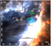 |
Fig. 1 Far-infrared colour composite image of M17 based on Herschel PACS data. Blue: 70 μm, green: 100 μm, and red: 160 μm. The sources with circumstellar disks are shown in blue, those with IR excess longwards of2.5 μm in green, and the “naked” OB stars in black. We do not observe an obvious trend in extinction properties with the location in the region. |
2 X-shooter observations
We have obtained VLT/X-shooter (300−2500 nm; Vernet et al. 2011) spectra of 11 (pre-)main sequence (PMS) stars ranging in mass from 6 to 20 M⊙. We selected this sample from the list of candidate massive PMS stars reported by Hanson et al. (1997) and we determined their stellar and extinction properties, which are presented in Paper I. The location of the observed targets in M17 is shown in Fig. 1. With the exception of Fig. 10, throughout this paper we have colour-coded the M17 sightlines according to the properties of the stellar spectral energy distributions. The blue circles represent the sightlines towards objects withcircumstellar disks (gas+dust disks), the green triangles towards stars with IR excess longwards of 2.5 μm (dusty disks), and the black squares towards OB stars without detected circumstellar material. We reduced the spectra using the X-shooter pipeline (Modigliani et al. 2010) version 2.7.1 running under the ESO Reflex environment (Freudling et al. 2013) version 2.8.4. The flux calibration was obtained using spectrophotometric standards from the ESO database. We then scaled the NIR flux to match the absolutely calibrated VIS spectrum. The telluric correction was performed using the software tool molecfit v1.2.01 (Smette et al. 2015; Kausch et al. 2015). The data reduction and analysis are described in detail in Paper I.
We calculated the stellar properties of the objects with visible photospheres by fitting FASTWIND models (Puls et al. 2005; Rivero González et al. 2012) and obtained the total extinction in the V -band, AV, and the visual-to-selective extinction ratio, RV, by fitting the flux calibrated X-shooter spectra to Castelli & Kurucz (2004) models. The spectral type and extinction properties presented in Paper I are listed in Table 1. In this paper we compare the results obtained in Paper I where we use the Cardelli et al. (1989) extinction law to deredden the flux calibrated spectra with results obtained by using the Fitzpatrick & Massa (2007) parameterisation of the extinction curve. We also compare the extinction parameters obtained by SED fitting with that derived from the colour excess E(B–V) (see Sect. 3). We also list the RV value obtained from Eq. (1); for objects with a NIR excess (i.e. a circumstellar disk: B243, B268, and B275) we iterated this equation starting with AK = 0. In this way we obtain an estimate of the K-band extinction AK, and thus a measure of the NIR excess (Sect. 3).
Extinction properties measured in the sightlines towards M17.
3 Extinction towards M17
By dereddening the SEDs of a dozen OB stars Hanson et al. (1997) detected a significant spread in both visual extinction AV (3–15 mag) and in total-to-selective extinction RV (2.8–5.5). They point out that the nebulosity disappears at the centre of the region and that the highest extinction is measured at the edges of this void. They also note that the DIB strengths (4430 and 4502 Å) do not show a significant increase even thoughthe visual extinction towards these objects varies from 3–10 mag. Earlier studies indicated that RV = 4.9 (Chini & Kruegel 1983) based on NIR photometry (but without knowledge of the spectral types), and RV = 3.3 using the maximum polarisation relation for RV (Schulz et al. 1981). Hoffmeister et al. (2008) concluded that the foreground extinction, with AV ~ 2 mag and RV = 3.1, differs from the extinction local to M17 for which they measure RV = 3.9 ± 0.2.
3.1 Dust extinction
In Paper I we constructed the spectral energy distribution (SED) of the stars by dereddening the X-shooter spectrum complemented with available photometric data. In order to deredden the spectrum we used the Cardelli et al. (1989) extinction law. We then constrained AV and RV towards the objects in M17 by fitting the slope of their SED in the photospheric domain (400–820 nm) to Castelli & Kurucz models2 (Kurucz 1993; Castelli & Kurucz 2004) corresponding to the spectral type given in Table 1.
The obtained values for RV range from 3.3 to 4.7 and AV varies from ~6 to ~15 mag. We do not find a significant correlation of the extinction properties with the position of the stars in the star-forming region. Cardelli et al. (1989) mention that their parameterisation of the extinction law becomes inaccurate when RV is large. As an example they refer to the sightline to Herschel 36.
As we know the spectral type of the targets, we can compare the value of the colour excess E(B–V) ≡ AV∕RV measured by fitting the SED with the value obtained directly by comparing the observed magnitudes to the intrinsic ones (E(B–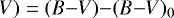 ). We adopt an error of 0.1 mag in E(B–V) in order to account for the uncertainty in the spectral classification and the photometric errors. For the main sequence stars we took the value of B0 and V0 from Pecaut & Mamajek (2013). For the giants we used the calibration in Wegner (2000, 2014). The comparison is shown in the left panel of Fig. 2. The value of E(B–V) derived from the SED fitting method is systematically higher than the one obtained directly from the observed and the intrinsic colours. The E(B–V) values obtained with the SED fitting method and the Fitzpatrick (1999) extinction law are closer to those obtained directly from the colours and we do not observe a systematic trend. Apparently, we underestimate the value of RV with the SED fitting method and the Cardelli et al. (1989) extinction law.
In order to investigate this further, we calculated RV using the relation reported in Fitzpatrick & Massa (2007):
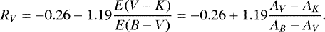 (1)
(1)
Given that this relation uses the K-band magnitude, it implicitly assumes that the target’s SED does not include an IR excess or, alternatively, that this is corrected for. In the case of the three objects with circumstellar disks (blue dots in the plots), we calculated RV by iterating Eq. (1). With AV = V − V0 and  , we started assigning a value of AK = 0 and calculated RV from this equation; we then used Fitzpatrick’s extinction law to calculate AK with the obtained RV and repeated this process until the values for both RV and AK converged. We arrived at RV = 4.6, 3.3, and 3.1 for B243, B268, and B275, respectively3. The comparison between the colour excess calculated with Fitzpatrick’s extinction law and the excess based on the observed and intrinsic colour is shown in the right panel of Fig. 2. From the figure it is clear that the value obtained using these two methods agree within the errors. In the case of objects with near-IR excess, we note that these two methods are not completely independent because we used the value based on the observed and intrinsic colour as initial guess to iterate Eq. (1).
We conclude that with the method used in Paper I, where the Cardelli et al. (1989) extinction law is used to deredden the SEDs for sightlines with high RV, we underestimate the value of this parameter. Furthermore, we observe that the values for AV obtained with the three methods agree with each other. This means that we did not make a significant error when calculating the luminosity of the objects in Paper I.
We do not find a systematic difference between the values obtained for objects with circumstellar gaseous disks (blue dots), only dusty disks (green triangle), and naked OB stars (black squares).
In the remainder of this paper we will adopt the values of AV = V −V0,  , and RV derived from Eq. (1).
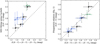 |
Fig. 2 Left panel: colour excess E(B–V) derived fromSED fitting (AV∕RV, Paper I) vs. the value obtained using the observed and the intrinsic colour |

3.2 Gaseous component of the extinction
The Ca II, Na I, and K I interstellar lines are shown in Fig. 3; we have overplotted the DIB at 5780 Å. The velocities have been corrected into the barycentric rest frame. In Table 2, we list the local standard rest (LSR) frame velocity measured for each of the lines. These radial velocities are consistent with interstellar absorption at distances of 1.3–2.2 kpc based on Galactic rotation models by Reid et al. (2009). We observe hardly any difference from one sightline to another. The atomic lines are mostly unresolved at the moderate X-shooter spectral resolution of R ~ 11 000. Although inconclusive regarding the exact distribution of gas in these lines of sight, these data indicate that the main gaseous absorption features are associated with M17 at ~2 kpc.
From 3D dust extinction maps (Drimmel et al. 2003) we find that the predicted visual extinction up to 1.8 kpc in the direction of M17 (i.e. in the foreground) corresponds to roughly 2 mag (or E(B–V) = 0.65 mag for a canonical value RV = 3.1), which is consistent with Hoffmeister et al. (2008). From the E(B–V) versus distance towards M17 plot obtained via the online tool STILISM4 by Capitanio et al. (2017) we obtain a value of E(B–V) = 0.78 mag at the distance M17, which is in line with our result. This plot shows that there are diffuse clouds in the foreground to the local gas and dust associated with the M17 region.
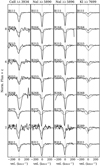 |
Fig. 3 Velocity profiles for the Ca II, Na I, and K I lines (black). We have overplotted the DIB at 5780 Å for reference (grey). The velocities are in the barycentric rest frame. The interstellar (gaseous) absorption profile is very similar from one sightline to another, and is likely due to a single cloud. |
4 Diffuse interstellar bands
In this section, we provide an overview of the DIB properties measured in the sightlines to the young OB stars in the star-forming region M17. We analysed the nine strongest DIBs present in the spectra obtained by the UVB and VIS arms of X-shooter (at 4430, 5780, 5797, 6196, 6284, 6379, 6614, 7224, and 8620 Å). We also included the NIR DIBs at 11797 and 13176, first reported by Joblin et al. (1990), and the one at 15268 (Geballe et al. 2011; Cox et al. 2014). The DIB equivalent width (EW) and full width at half maximum (FWHM) are listed in Table 3. The first column corresponds to the central wavelength of the DIBs; the top values show the FWHM in nm, and the bottom values show the EW measurements in (mÅ).
We also detect the 9577 and 9632 DIBs whose carrier has recently been identified in the laboratory to be the  molecule (Campbell et al. 2015). The FWHM and EW of these two DIBs are displayed in rows 10 and 11 of Table 3.
We searched for the presence of CH+ and CH at 4232, 4300 Å, but given the signal-to-noise ratio of our data at such blue wavelengths we were not able to detect these molecules inthe X-shooter spectra.
Local standard rest frame (LSR) radial velocities obtained from a Gaussian fit to the Ca II, Na I, and K I interstellar lines in each line of sight.
4.1 DIB strengths and widths
The EW was measured by integrating the flux of each DIB within the boundaries shown in Appendix A. The error on the EW was calculated following the method described in Vos et al. (2011): 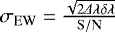 , where Δλ is the integration range and δλ is the spectral dispersion. The real errors might be larger due to unknown systematic uncertainties, particularly regarding the continuum normalisation. The S/N was measured in the shaded region, and is shown in Appendix A. The FWHM (
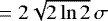 ) of each DIB was measured by fitting a Gaussian function to the absorption lines.
4.2 Correlation between EW(6196) and EW(6613)
In order to check the consistency of the measurements we show our data, together with literature data, for the strongly correlated DIBs at 6614 and 6696 Å in Fig. 4 (McCall et al. 2010; Krełowski et al. 2016). The dashed line shows a linear fit to the data by McCall et al. (2010) and the grey region shows the 1σ error on the fit. The measured ratios are in agreement with the trend observed in other Galactic sightlines.
4.3 C bands
bands
We measured the C bands at 9577 and 9632 Å. The EW of the 9577 DIB increases roughly with AV. B331 is an outlier with relatively weak 9577 and 9632 Å DIBs. The average measured 9632/9577 ratio is 1.1, which is higher than the ratio 0.8 expected from laboratory measurements. The 9632 Å DIB is known to suffer from contamination by a photospheric Mg II line. However, unless there are other factors impacting this ratio in M17, the stellar contamination has to be, on average, higher than 150 mÅ in order to reduce the observed ratio to 0.8. This appears to require a rather large contribution from photospheric Mg II and we note that we cannot exclude systematic errors originating from telluric residuals.
In the optically thin limit the EW of the 9577 Å DIB can be converted into a column density. We do not use the 9632 Å DIB as it is known to suffer from photospheric line contamination which is difficult to correct for. For the observed 9577 Å DIB strengths this gives N(C ) = 2.5–4.3 × 1013 cm−2. These are somewhat lower abundances than the neutral C60 abundance of 2.4 × 1014 cm−2∕G0, where G0 is the radiation field, measured with Spitzer in the diffuse ISM (Berné et al. 2017). However, the higher sensitivity of JWST opens the possibility to detect fullerene infrared emission (potentially both C60 and C
 features) towards M17 that would allow a comparison between emission and absorption measurements in the same environment.
DIB properties in the lines of sight to M17.
4.4 DIB profiles
Dahlstrom et al. (2013) reported on anomalous DIB profiles in the sightline towards Herschel 36. According to the authors, the profiles of the 5780, 5797, 6196, and 6614 DIBs show an extended red wing in comparison to nominal sightlines. Oka et al. (2013) confirmed this finding for three of the DIBs, but did not detect a pronounced red wing in the DIB at 6196 Å (we also do not detect a red wing in the profile of the 6196 DIB with the lower-resolution X-shooter data). These authors performed a study that allowed them to make a distinction between the carriers of the above DIBs at 5780, 5797, and 6614 DIBs and others (e.g. 5850, 6196, and 6379) which do not present such a pronounced red wing.
In addition, the sightline towards Herschel 36 shows absorption lines from rotationally excited CH+ and CH and from vibrationally excited H2. Furthermore, an atypical extinction curve is observed with RV ~ 6 and a weak 2175 Å bump, i.e. a flat far-UV extinction curve (Dahlstrom et al. 2013). M17 also shows anomalous extinction (RV > 3.1; Paper I); therefore, it is a good candidate to search for anomalous behaviour in the DIBs.
We compare the profiles of the DIBs towards M17 with those observed in the direction of Herschel 36 and HD 161061 (a nominal sightline) in Fig. 5. The X-shooter spectra of Herschel 36 (unpublished) and the nominal sightline (HD 161061) were obtained previously by us with ESO programs 091.C-0934(B) and 385.C-0720(A). The spectra for these two sources were reduced using the same procedure described in Sect. 2.
To facilitate the comparison, we scaled the flux of the DIBs towards Herschel 36 and HD 161061 to match the depths of the cores of the DIBs towards M17. The profiles of the DIBs towards M17 are similar to the “nominal” profile, and they do not show a red wing like that in the case of Herschel 36. In the case of the 6196 Å DIB we do not detect a red wing in the spectrum of Herschel 36.
 |
Fig. 4 Correlation between the DIBs at 6614 and 6196 Å. The dashed line represents the relation found by McCall et al. (2010; grey dots) and the grey area shows the 1σ errors to the fit. The blue circles represent the sightlines towards objects with circumstellar disks, the green triangles towards stars with IR excess longwards of 2.5 μm, and the black squares towards OB stars. |
5 Comparison with other sightlines
For reddened lines of sight the strength of many DIBs increases in a roughly linear way with E(B−V). The relation between the DIB strength and the reddening is not very well constrained for high extinction values because of the lack of data covering those high values of E(B−V). Also, these studies have been applied to only a few prominent DIBs, mostly the 5797, 5780, and 6614 Å DIBs.
In Fig. 6, we compare the strength of some prominent DIBs in M17 as a function of the reddening E(B−V) with that inother published studies. We plot a linear fit to a large variety of Galactic sightlines (Chlewicki et al. 1986; Benvenuti & Porceddu 1989; Herbig 1993; Sonnentrucker et al. 1997; Krełowski et al. 1999; Tuairisg et al. 2000; Rawlings et al. 2003; Galazutdinov et al. 2004; Cox et al. 2005; Friedman et al. 2011, for details see figure captions) excluding the star-forming regions (M17, Herschel 36, and RCW 36) for the three DIBs mentioned above with dashed black lines. With the grey area we show the linear fit and the 1σ error bars to the fit. For reference, we also plot DIB equivalent width measurements for Herschel 36 and for the massive star-formingregion RCW 36 (Ellerbroek et al. 2013). The large scatter on these relations is intrinsic due to physical variations between lines of sight, and not due to measurement uncertainties. For example, Vos et al. (2011) show that there is a dichotomy in the DIB strength versus extinction relation for UV exposed and UV shielded environments.
The M17 points are located below the average Galactic trend, like the sightlines probing the dense Cyg OB2 region. On the other hand, when including the DIBs towards M17 in the fit, the slope of the relation does not change significantly for each of the three DIBs.
We also compared the strength of the NIR DIB at 15 268 Å as a function of E(B–V) with severalGalactic sightlines taken from the SDSS-III APOGEE survey by Zasowski & Ménard (2014). We do not showthis comparison, but we observe that the sightlines towards M17 follow the same trend as those observed in different Galactic environments. We conclude that the DIB behaviour with respect to reddening E(B−V), as observed in the direction of M17, indicates that these sightlines probe a denser ISM, but are not peculiar.
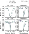 |
Fig. 5 Comparison of the shape of some DIBs towards M17 (B111, green solid line) with the sightline towards Herschel 36 (purple dotted line) and a “nominal” sightline (black dashed line). All the spectra have been convolved to the same resolution and scaled to have the same line central depth. The M17 DIB profiles do not show an extended red wing or any other anomaly with respect to the DIB in HD 161061. |
5.1 Ratio of EW(5797) to EW(5780)
Vos et al. (2011) demonstrated that the ratio 5797/5780 might be useful to distinguish between sightlines probing diffuse cloud edges and denser cloud cores. The 5797 Å DIB is less sensitive to UV radiation than the 5780 Å DIB; therefore, we expect that the 5797/5780 ratio would be lower in higher extinction environments. This effect is strongest in sightlines dominated by one velocity component in the interstellar gas absorption profile (i.e. single-cloud sightlines) and tends to get “washed-out” in multi-cloud sightlines. The EW ratio of the 5797/5780 DIBs is plotted in Fig. 7. Compared to the lower extinction data (E(B−V) < 1 mag; Friedman et al. 2011; Vos et al. 2011) the DIBs towards M17 cover a smaller range (0.15–0.45) in the 5797/5780 DIB ratio (though at higher extinction values). We do not find a clear correlation with spatial location in the cloud. We note that the interstellar gas absorption features of Ca II and Na I are largely unresolved at the spectral resolution of X-shooter. It is conceivable that at higher spectral resolution the interstellar gas component associated with M17 will be resolved in multiple velocity components. This could imply that due to averaging along the line of sight the observed 5797/5780 ratio constitutes an average of this ratio in individual clouds. Variations of 5797/5780 (in diffuse ISM) are thought to depend strongly on the local geometry and the effective UV radiation field (see above), both of which are complex within the large H II region. Additionally, variations in the 5797/5780 ratio in the densest regions (high RV) can potentially be driven by different mechanisms (e.g. depletion) compared to changes in this ratio in the more diffuse medium (e.g. effective UV radiation field); this could be the case for M17 as the change on strength (per AV) of these two DIBs with RV is different from each other as shown in Fig. 10 and discussed in Sect. 6.
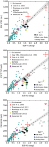 |
Fig. 6 Equivalent width of the 5780 (top panel), 5797 (middle panel), and 6614 Å (bottom panel) DIBs as a function of reddening E(B−V) for Galactic sightlines. The DIB strengths are taken from the literature (open symbols) and this work (filled symbols). The dashed line indicates the linear fit for the Galactic sightlines excluding the star-forming regions (RCW 36, Herschel 36, and M17), and the grey area represents the 1σ error on the fit. |
 |
Fig. 7 Ratio of the 5797 to 5780 DIBs. The open symbols show data from the literature and the filled symbols data from the sightlines towards M17. The dashed line represents the division between ζ- and σ-type clouds. |
5.2 8620 DIB
The DIB at 8620 Å has recently gained more attention because it has been included in the large-scale surveys of RAVE and Gaia. It has been shown that the EW of this DIB is well correlated with the colour excess E(B–V); Munari et al. (2008) reported a relation between the DIB strength and E(B–V) given by E(B–V) = (2.72 ± 0.03) ×EW 8620 Å for E(B–V) < 1.2.
Maíz Apellániz et al. (2015) measured this DIB in two sightlines with high extinction towards O stars in the cluster Berkeley 90. The authors detect at least two clouds moving at different velocities towards these objects; one thinner cloud associated with the material far away from the stellar cluster, and a thicker one associated with the material local to the cluster. The latter cloud is thicker for one sightline, which allowed the authors to measure the properties of DIBs in σ (RV ~ 4.5) and in ζ (RV ~ 3.1) clouds (see Sect. 5.1 for details about σ and ζ clouds). They observed that the DIB at 8620 Å is highly depleted in dense clouds and, therefore, correlates poorly with extinction higher than AV ~ 6.
Damineli et al. (2016) extended the correlation of the 8620 DIB with extinction by adding sightlines with higher values of AK. They used the extinction in the K band because it is less sensitive to the grain size than AV. They adopted AKs = 0.29 E(B−V), which allowed the Munari et al. (2008) relation to be expressed as AKs = (0.691) × EW 8620 Å. They find the following correlation:
 (2)
(2)
This is in good agreement with Munari et al. (2008) for EW < 0.6 Å, which translates to AV < 9 mag for the extinction properties of their sample.
Using data from the RAVE survey, Kos et al. (2014) measured the strength of the 8620 Å DIB for ~500 000 spectra at distances <3 kpc. We plot the EW of the 8620 Å DIB in Fig. 8. We include the data by Damineli et al. (2016, red dots) and Kos et al. (2014, grey dots), the black dashed line and the blue shadow represent the relation in Eq. (2). In order to derive AK from the Kos et al. (2014) data, we adopted AK∕AV = 0.11.
The DIB strength towards M17 shows a very large spread in comparison with the relation by Damineli et al. (2016). This spread is similar to that observed in the sightlines from the RAVE survey. The large scatter in the M17 data could be an indication that the DIB carrier becomes depleted at extinctions AK > 1.0. We detect a general positive correlation between the strength of the 8620 DIB and the K-band extinction for AK ≲ 1.0.
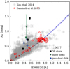 |
Fig. 8 K-band extinction AK vs. strength of the DIB at 8620 Å. The open symbols show data from the literature, and the filled symbols sightlines towards M17. The dotted line and the blue area show the relation in Eq. (2). |
6 DIB strengths versus RV
The value of RV is related to the size distribution of the dust grains. High values of RV imply a relative over-abundance of large grains, whereas low RV values indicate that the small dust grains are more dominant in the size distribution. Typically higher values of RV are associated with denser clouds where grain growth is or has been more significant than in diffuse regions. This is reflected in the relative slope of the extinction curve. Higher RV values correspond to a flatter extinction curve, meaning that photons at all wavelengths are more equally absorbed.
Cardelli et al. (1989) presented observational evidence that the 2175 Å feature, normalised by the amount of extinction, shows a positive trend with  . In Fig. 9 we present a similar plot based on measurements recently collected by Xiang et al. (2017). Although the plot reveals significant scatter, there appears to be a general trend that sightlines with a lower value of RV show a stronger 2175 Å feature per magnitude visual extinction. The Pearson correlation coefficient between EW(2175Å) and
  has a value of r = 0.3, which indicates a rather weak formal correlation.
In Fig. 10 we plot the strength of the DIBs normalised by the visual extinction AV with  . We include the sightlines towards M17, Herschel 36, and the object 408 in RCW 36. Where available, we add the data from Xiang et al. (2017) who compiled the EW of several DIBs in 97 sightlines. For most DIBs we discern a positive trend of the normalised DIB strength (EW/AV) with
  , similar to the trend seen for the 2175 Å feature (Fig. 9). Given that AV is in the denominator of both axes, if the uncertainties in AV are large, a spurious relation between EW/AV and
  might result. This is because when dividing by a very uncertain AV, we expect some values of both EW/AV and
  to be very low and some to be very large causing a spurious linear relation intercepting at zero. However, we consider the errors in AV to be small enough – primarily due to the accurate determination of the spectral type – that we do not expect such an effect here.
We note that there is a cloud of data points centred at the Galactic average value of RV = 3.1. The observed scatter could represent sampling of non-heterogeneous (multiple) interstellar cloud conditions in these sightlines. In other words, variations in DIB band strength (per unit reddening) are more pronounced than variations in average dust grain size. The presence of this cloud of data points shows that normalising by AV does not introduce a spurious relation. If that were the case, we would expect the points at all RV values to follow a linear relation. On the other hand, for sightlines with RV ≿ 3.8 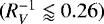 there appears to be a much more pronounced (linear) relation between EW/AV and
  . The M17 data presented here strengthen the presence of this linear relation that can already be gleaned from the data compiled by Xiang et al. (2017) where most of the sightlines with RV ≿ 3.8 correspond to stars in star-forming regions (Orion giant molecular cloud, Upper Scorpius, Triffid nebula, and Rho Ophiuchi).
We performed an orthogonal distance regression (ODR; Churchwell 1990)5 to fit a linear function to the DIB strength normalised by the visual extinction AV versus  for sightlines towards M17. The fit results, together with the Pearson correlation coefficients are listed in Table 4 and shown in Fig. 10, where the black line corresponds to the best fit to the M17 data alone and the shaded region to the 1σ error on the fit.
Based on the results from the fit, we confirm that for M17 there is a linear relation between the normalised DIB strength and  . This correlation is strongest for the DIBs at 5780, 6196, 6284, 6614, and 9632 Å. From the Pearson correlation coefficient, r, we find that the correlation is moderate to strong (r > 0.6) for all DIBsexcept for those at 4430, 6379, 11797, and 13 176 Å where the correlation is weak (r < 0.5). We note that for the 11 797 and 13 176 Å DIBs there is a clear outlier data point which strongly affects the Pearson correlation coefficient r (Fig. 10). This point corresponds to the B275 sightline where the spectral quality in the ranges of these two DIBs is poor, which could introduce systematic errors in the DIB measurements (see Figs. A.12 and A.13). Excluding this point results in r > 0.7 for both DIBs.
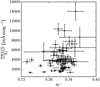 |
Fig. 9 Normalised EW of the 2175 Å feature measured in Galactic sightlines as a function of RV. The measurements are obtained from Xiang et al. (2017). The 2175 Å feature is stronger in sightlines characterised by a lower value of RV. |
Results of the linear fit of EW/AV vs.  towards M17 sightlines.
7 Discussion and conclusion
7.1 Extinction in M17
We calculated the extinction properties of the sightlines towards M17, with overall relatively high RV values, using different methods: i) by dereddening the SED of the stars using Cardelli’s extinction law and then fitting it to Kurucz models to find AV and RV (from that E(B–V) = AV∕RV); ii) by directly comparing the intrinsic magnitudes to the observed values to find AV and E(B–V) (RV = AV∕E(B − V)); and iii) by finding AV and E(B–V) from the intrinsic and observed magnitudes and calculating RV, as defined by Fitzpatrick & Massa (2007; Eq. (1)). We observe that the colour excess E(B–V) calculated with Cardelli’s extinction law and the SED fitting is systematically higher than when using the other two methods. This confirms that this extinction law is not well suited for high values of RV, as already stated in Cardelli et al. (1989). We conclude that the best way of obtaining the extinction properties is to use the intrinsic and observed magnitudes and then calculate RV as shown in Eq. (1), because with this equation it is also possible to take into account the NIR part of the SED.
7.2 Relation of DIBs with E(B–V)
In Fig. 6, we show the relation of the DIBs at 5780 and 5797 Å with the colour excess E(B–V) in M17 and compare it with other sightlines published in the literature. The value of E(B–V) for the sightlines in M17 is relatively high compared to other Galactic sightlines; nevertheless, the DIB strength seems to follow the same trend as observed in other reddened sightlines.
Ellerbroek et al. (2013) reported an anomalous behaviour of the DIB strength in sightlines towards the star-forming region RCW 36. We do not find a similar deviation in the sightlines towards M17. The behaviour reported in RCW 36 could be due to the way in which the authors calculated AV. They assumed a value of RV = 3.1, dereddened the spectrum using Cardelli’s extinction law, and then fitted it to Kurucz models. In this paper we show that the value of E(B–V) can be overestimated by as much as 0.5 mag (Fig. 2) when using Cardelli’s extinction law. Previous studies have shown that star-forming regions such as M17 and M8 (where Herschel 36 resides) often show high values of RV (e.g. Cardelli et al. 1989; Hanson et al. 1997). Therefore, the assumption that RV = 3.1 for RCW 36 probably underestimates its true RV.
7.3 Relation of DIBs with RV
The observed trend of EW(DIB)/AV with  for M17 and other sightlines with RV ≿ 3.8 (
 ; cf. Fig. 10) is reminiscent of what Cardelli et al. (1989) and Xiang et al. (2017) find for the 2175 Å bump, the carrier of which is thought to consist of some (unidentified) carbonaceous material; however, the trend of the bump is weaker than that observed forthe DIBs.
The slope of the linear relation between EW/AV and  (valid for RV ≳ 3.8) can be interpreted as a measure of the sensitivity to which variations in the abundance of DIB carriers (per unit visual extinction) are related to variations in the average grain size of interstellar dust. This slope can then be interpreted in the context of either the depletion of the DIB carrier as the dust grains coagulate and grow (see e.g. Jura 1980; Ormel et al. 2009, EW/AV decreases while RV increases) or the production of DIB carriers as the larger grains get destroyed by the increasingly effective UV radiation field (see e.g. Cecchi-Pestellini et al. 1995; Jones 2004, EW/AV increases and RV decreases).
Alternatively, in the hypothesis that some DIB carriers are ionised species, the strengths of DIBs are expected to increase with a stronger effective UV radiation field. If RV could be regarded as a tracer of the effective UV radiation field, higher values correspond to a lower ionisation fraction, hence lower EW/AV. In this context the slope of EW/AV versus  would be directly related to the ionisation potential of the carrier species.
With the current data we cannot distinguish between these different scenarios. However, it is possible to identify groups or families of DIB carriers which behave similarly in the transition from the more dense to diffuse ISM (high to low RV). To investigate this we compared the column density of the DIB carriers multiplied by the (unknown) oscillator strength, Nf, with the slope d(EW/AV)/d (cf. Fig. 10; Table 4). This slope can be viewed as a measure of the sensitivity of the DIB carriers to changes in
  , hence in grain size distribution or as a measure of the carrier’s ionisation potential. We refer to this slope as the DIB–RV sensitivity. Assuming that the optically thin approximation holds for the DIBs (no saturation of absorption) we have
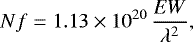 (3)
(3)
where N is the column density in cm−2, f the oscillator strength, EW is the equivalent width (in Å) and λ is the central wavelength of each DIB (in Å). We show the dependence of the DIB–RV sensitivity on Nfλ2, and Nf in Fig. 11; In both cases a linear fit is shown with a dashed line and the shaded region shows the 2σ error to the fit. Additionally, we marked the  DIBs with green pentagons.
First we discuss the results in the context of RV as a proxy for changes in the grain size distribution. We are able to identify two groups; the first group contains ten moderately strong DIBs: the two  DIBs, the DIBs presenting a red wing in Herschel 36 (5780, 5797, and 6614), and those at 6196, 6379, 7224, 8620, and 11797 Å. These DIBs show a modest sensitivity to the change in grain size, and their sensitivity increases almost linearly as a function of DIB strength. The second group consists of four strong DIBs (at 4430, 6284, 13176, and 15268 Å) that are very sensitive to the change in grain size distribution (large d(EW/AV)/d
 slope values), but their DIB-RV sensitivity does not seem to depend on the DIB strength.
In the case of the first group, we postulate that the observed linear increase in the DIB-RV sensitivity with the amount of DIB carriers, Nf, suggests that the increase in the latter is primarily due to an increase in column density and that f is quite similar for this group of DIB carriers. This is because the reverse situation, i.e. that a systematic increase in the sensitivity of DIB carriers to changes in RV is related to a systematic increase in the oscillator strength of the DIB carriers appears much more unlikely. If this is the case, the oscillator strengths of these DIBs could be extracted with reference to the two DIBs at 9577 and 9632 Å assigned to C (f9577 = 0.018 and f9632 = 0.015).
The linear dependency of the DIB-RV sensitivity on the DIB strength implies that the relative production/destruction rate of these DIB carriers is the same for the same change in typical grain size (RV). In other words, for a doubling of the abundance of DIB carriers in the first group, the same change in grain size distribution is required. This may imply a common production/destruction mechanism. The fact that the DIB-RV sensitivity of the stronger DIBs is independent of their strength suggests the existence of an additional reservoir of DIB carriers unrelated to the dust grains. These carriers would be produced or destroyed as the grain size distribution changes and via other mechanisms.
Alternatively, we consider the scenario where RV is a proxy of the effective UV radiation field strength and the DIB carriers are large ionised molecules. In this case Fig. 11 has to be interpreted differently. Here the slope d(EW/AV)/d is an indirect measure of the carrier’s ionisation potential. The broad DIBs at 15 268, 13 176, 6284, and 4430 Å have a (similar) strong slope which implies a (similar) low ionisation potential. The ionisation potential of the carriers of these broad DIBs is then expected to be significantly lower than the ionisation potential of 7.58 eV measured for C60 (de Vries et al. 1992). In the opposite direction, the narrow DIBs at 7224, 5797, 6614, 6196, and 6379 Å which have increasingly shallower slopes should then have increasingly higher ionisation potentials. For PAHs the ionisation potential is strongly related to their number of π-electrons (see Fig. B.1. in Ruiterkamp et al. 2005).
We note that in the case that there are several foreground clouds contributing to the extinction in the sightline towards M17, the interpretation of the observed relations is complicated. The hypotheses presented above assume that most of the variation in AV and RV arises from the dust and gas in the M17 region. Correcting for a foreground sheet of dust, with AV = 2 and a constant foreground EW(DIB)/AV contribution projected across the M17 region, would shift all the EW/AV values vertically. Also, correcting for foreground dust with a nominal RV = 3.1 will sightly increase the RV values derived for the local M17 dust, but will have little impact on the slope of the relation between EW(DIB)/AV and  . It could also affect the mean normalised line strengths. The above scenarios and hypotheses can be further tested by examining the relation between EW(DIB)/AV and RV for other star-forming regions that probe a range of extinction properties and grain size distributions, similar to M17. This will also help to disentangle the impact of foreground dust extinction and to determine possible effects due to measurement uncertainties.
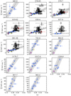 |
Fig. 10 Normalised DIB EW vs. |


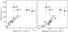 |
Fig. 11 Slope representing the sensitivity of EW/AV with changesin |


8 Summary
We present an analysis of the properties of the DIBs in sightlines towards the star-forming region M17 in comparison to the properties of nominal DIBs and of DIBs that have been reported to be anomalous. Our findings can be summarised as follows:
- 1.
Cardelli’s extinction law is not suitable for high values of RV. The best way of calculating the extinction parameters AV and E(B–V), when the spectral type of the observed star is known, is by directly comparing the observed and intrinsic magnitudes. By using the relation between RV and E(V −K)∕E(B−V) of Fitzpatrick & Massa (2007) it is possible to calculate AK and, therefore the K-band excess produced by the circumstellar disk.
- 2.
From the observed C
 DIB at 9577 Å we derive a column density N(C
 ) = 2.5 − 4.3 × 1013 cm−2.
 - 3.
We also detect the NIR DIBs at 11 797, 13 176, and 15 268 Å in the sightlines towards M17.
- 4.
The profiles of the DIBs towards M17 do not present a red wing in contrast to those towards Herschel 36. This indicates that the red wing is not common to star-forming regions, and that the environment towards Herschel 36 must present some special properties that cause the DIBs to have a red wing.
- 5.
The strength of the 5780 Å DIBs towards M17 is as expected from the relations found in the literature for their values of E(B–V). The 5797 Å DIBs show a relatively large spread in relation to other Galactic DIBs, and the 6614 Å DIBs towards M17 are slightly weaker than expected for their E(B–V) values.
- 6.
In the M17 region we find trends between the strength of the studied DIBs (per unit visual extinction) and
 , most notably for the 6196 and 7224 Å DIBs. The trend remains when we include the sightlines towards star-forming regions presented in Xiang et al. (2017). For sightlines with RV ~ 3.1 there is no trend.
 - 7.
The slope values of the linear relation between the DIBs EW normalised by AV and
 (DIB-RV
sensitivity) allow us to identify two main groups of DIBs in terms of their sensitivity to RV
(for RV > 3.8,
(DIB-RV
sensitivity) allow us to identify two main groups of DIBs in terms of their sensitivity to RV
(for RV > 3.8,
 ). The first group consists of DIBs with similar sensitivity to changes in RV
as the two
). The first group consists of DIBs with similar sensitivity to changes in RV
as the two  DIBs: 5780, 5797, 7224, 8620, 9577, 9632, and 11 797 Å. For this group we find that the DIB-RV
sensitivity varies linearly with DIB strength. The second group consists of DIBs with roughly three times stronger DIB-RV
sensitivity: 4430, 6284, 13 176, and 15 268 Å; for this group, the DIB-RV
sensitivity does not depend on the DIB strength. This response of DIB carriers to changes in interstellar dust properties provides additional clues to the (dis)similarity of different DIB carriers, and may provide clues to their production/destruction mechanisms, and can thus ultimately help with their identifications.
DIBs: 5780, 5797, 7224, 8620, 9577, 9632, and 11 797 Å. For this group we find that the DIB-RV
sensitivity varies linearly with DIB strength. The second group consists of DIBs with roughly three times stronger DIB-RV
sensitivity: 4430, 6284, 13 176, and 15 268 Å; for this group, the DIB-RV
sensitivity does not depend on the DIB strength. This response of DIB carriers to changes in interstellar dust properties provides additional clues to the (dis)similarity of different DIB carriers, and may provide clues to their production/destruction mechanisms, and can thus ultimately help with their identifications. - 8.
Three scenarios are proposed for the observed behaviour of DIBs in star-forming regions (with RV > 3.8): (1) DIBcarriers stick to dust grains, and thus get depleted from the gas phase as the grains grow in size (dust-coagulation) in the denser regions of interstellar clouds; (2) DIB carriers are produced from the dust grains in the strong UV radiation fields in these regions which lead to increased abundances of DIB carriers (and that of the 2715 Å band) and, by direct consequence, a decrease in the average dust particle size; (3) as RV decreasesand the effective UV radiation field strength increases the ionisation fraction of the parent carriers increases, thus causing the DIBs related to ionised molecular carriers to become stronger. The effective response of DIB strength to changes in the UV radiation field, i.e. d(EW/AV)/d
 , is then ameasure of the carrier’s ionisation potential. At this point we cannot distinguish between these scenarios. Further investigations of specific (star-forming) regions that probe a range of RV
values, like M17, are needed to examine the relation between DIB strength and RV.
, is then ameasure of the carrier’s ionisation potential. At this point we cannot distinguish between these scenarios. Further investigations of specific (star-forming) regions that probe a range of RV
values, like M17, are needed to examine the relation between DIB strength and RV.
Acknowledgements
Based on observations collected at the European Organisation for Astronomical Research in the Southern Hemisphere under ESO programmes 091.C-0934(B) (Herschel 36), 385.C-0720(A) (HD161056), 60.A-9404(A), 085.D-0741, 089.C-0874(A), and 091.C-0934(B) (M17). The authors thank Rens Waters, Martin Heemskerk, Juan Hernandez Santisteban, Lucia Klarmann, Samayra Straal, Marieke van Doesburgh, Xander Tielens, and Rosine Lallement for discussions that helped to improve this paper. This research made use of Astropy, a community-developed core Python package for Astronomy (Astropy Collaboration 2018), NASA’s Astrophysics Data System Bibliographic Services (ADS), and the SIMBAD database, operated at CDS, Strasbourg, France (Wenger et al. 2000).
Appendix A Observed DIBs and Gaussian fits
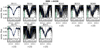 |
Fig. A.1 DIB profiles at 4430 Å. The vertical dashed lines show the integration limits used to calculate the DIB strength, the dotted line shows the central wavelength of the DIB, and the green shaded area shows the region in which the error was calculated. We show the Gaussian fit to the DIB profile with a solid blue line. The white box at the bottom of each panel indicates the FWHM and EW of this DIB for each object. |
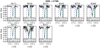 |
Fig. A.2 DIB profiles at 5780 Å. The vertical dashed lines show the integration limits used to calculate the DIB strength, the dotted line shows the central wavelength of the DIB, and the green shaded area shows the region in which the error was calculated. We show the Gaussian fit to the DIB profile with a solid blue line. The white box at the bottom of each panel indicates the FWHM and EW of this DIB for each object. |
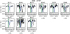 |
Fig. A.3 DIB profiles at 5798 Å. The vertical dashed lines show the integration limits used to calculate the DIB strength, the dotted line shows the central wavelength of the DIB, and the green shaded area shows the region in which the error was calculated. We show the Gaussian fit to the DIB profile with a solid blue line. The white box at the bottom of each panel indicates the FWHM and EW of this DIB for each object. |
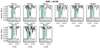 |
Fig. A.4 DIB profiles at 6196 Å. The vertical dashed lines show the integration limits used to calculate the DIB strength, the dotted line shows the central wavelength of the DIB, and the green shaded area shows the region in which the error was calculated. We show the Gaussian fit to the DIB profile with a solid blue line. The white box at the bottom of each panel indicates the FWHM and EW of this DIB for each object. |
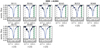 |
Fig. A.5 DIB profiles at 6284 Å. The vertical dashed lines show the integration limits used to calculate the DIB strength, the dotted line shows the central wavelength of the DIB, and the green shaded area shows the region in which the error was calculated. We show the Gaussian fit to the DIB profile with a solid blue line. The white box at the bottom of each panel indicates the FWHM and EW of this DIB for each object. |
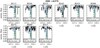 |
Fig. A.6 DIB profiles at 6379 Å. The vertical dashed lines show the integration limits used to calculate the DIB strength, the dotted line shows the central wavelength of the DIB, and the green shaded area shows the region in which the error was calculated. We show the Gaussian fit to the DIB profile with a solid blue line. The white box at the bottom of each panel indicates the FWHM and EW of this DIB for each object. |
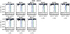 |
Fig. A.7 DIB profiles at 6113 Å. The vertical dashed lines show the integration limits used to calculate the DIB strength, the dotted line shows the central wavelength of the DIB, and the green shaded area shows the region in which the error was calculated. We show the Gaussian fit to the DIB profile with a solid blue line. The white box at the bottom of each panel indicates the FWHM and EW of this DIB for each object. |
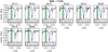 |
Fig. A.8 DIB profiles at 7224 Å. The vertical dashed lines show the integration limits used to calculate the DIB strength, the dotted line shows the central wavelength of the DIB, and the green shaded area shows the region in which the error was calculated. We show the Gaussian fit to the DIB profile with a solid blue line. The white box at the bottom of each panel indicates the FWHM and EW of this DIB for each object. |
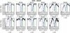 |
Fig. A.9 DIB profiles at 8620 Å. The vertical dashed lines show the integration limits used to calculate the DIB strength, the dotted line shows the central wavelength of the DIB,and the green shaded area shows the region in which the error was calculated. We show the Gaussian fit to the DIB profile with a solid blue line. The white box at the bottom of each panel indicates the FWHM and EW of this DIB for each object. |
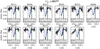 |
Fig. A.10 C |

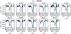 |
Fig. A.11 C |

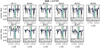 |
Fig. A.12 NIR DIB profiles at 11797 Å. The vertical dashed lines show the integration limits used to calculate the DIB strength, the dotted line shows the central wavelength of the DIB, and the green shaded area shows the region in which the error was calculated. We show the Gaussian fit to the DIB profile with a solid blue line. The white box at the bottom of each panel indicates the FWHM and EW of this DIB for each object. |
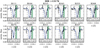 |
Fig. A.13 NIR DIB profiles at 13176 Å. The vertical dashed lines show the integration limits used to calculate the DIB strength, the dotted line shows the central wavelength of the DIB, and the green shaded area shows the region in which the error was calculated. We show the Gaussian fit to the DIB profile with a solid blue line. The white box at the bottom of each panel indicates the FWHM and EW of this DIB for each object. |
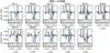 |
Fig. A.14 NIR DIB profiles at 15268 Å. The vertical dashed lines show the integration limits used to calculate the DIB strength, the dotted line shows the central wavelength of the DIB, and the green shaded area shows the region in which the error was calculated. We show the Gaussian fit to the DIB profile with a solid blue line. The white box at the bottom of each panel indicates the FWHM and EW of this DIB for each object. |
References
- Astropy Collaboration (Price-Whelan, A. M., et al.) 2018, AJ, 156, 123 [Google Scholar]
- Benvenuti, P., & Porceddu, I. 1989, A&A, 223, 329 [NASA ADS] [Google Scholar]
- Berné, O., Cox, N. L. J., Mulas, G., & Joblin, C. 2017, A&A, 605, L1 [NASA ADS] [CrossRef] [EDP Sciences] [Google Scholar]
- Broos, P. S., Feigelson, E. D., Townsley, L. K., et al. 2007, ApJS, 169, 353 [NASA ADS] [CrossRef] [Google Scholar]
- Cami, J., & Cox, N. L. J., eds. 2014, in The Diffuse Interstellar Bands, IAU Symp., 297 [Google Scholar]
- Campbell, E. K., Holz, M., Gerlich, D., & Maier, J. P. 2015, Nature, 523, 322 [NASA ADS] [CrossRef] [PubMed] [Google Scholar]
- Capitanio, L., Lallement, R., Vergely, J. L., Elyajouri, M., & Monreal-Ibero, A. 2017, A&A, 606, A65 [NASA ADS] [CrossRef] [EDP Sciences] [Google Scholar]
- Cardelli, J. A., Clayton, G. C., & Mathis, J. S. 1989, ApJ, 345, 245 [NASA ADS] [CrossRef] [Google Scholar]
- Castelli, F., & Kurucz, R. L. 2004, ArXiv e-prints [arXiv:astro-ph/0405087] [Google Scholar]
- Cecchi-Pestellini, C., Aiello, S., & Barsella, B. 1995, ApJS, 100, 187 [NASA ADS] [CrossRef] [Google Scholar]
- Chini, R., & Kruegel, E. 1983, A&A, 117, 289 [NASA ADS] [Google Scholar]
- Chini, R., Elsaesser, H., & Neckel, T. 1980, A&A, 91, 186 [NASA ADS] [Google Scholar]
- Chlewicki, G., van der Zwet, G. P., van Ijzendoorn, L. J., Greenberg, J. M., & Alvarez, P. P. 1986, ApJ, 305, 455 [NASA ADS] [CrossRef] [Google Scholar]
- Churchwell, E. 1990, in Contemporary Mathematics, Vol. 112, Hot Star Workshop III: The Earliest Phases of Massive Star Birth, ed. P. Brown & W. Fuller (American Mathematical Society) 186 [Google Scholar]
- Cox, N. L. J., Kaper, L., Foing, B. H., & Ehrenfreund, P. 2005, A&A, 438, 187 [NASA ADS] [CrossRef] [EDP Sciences] [Google Scholar]
- Cox, N. L. J., Cordiner, M. A., Ehrenfreund, P., et al. 2007, A&A, 470, 941 [NASA ADS] [CrossRef] [EDP Sciences] [Google Scholar]
- Cox, N. L. J., Cami, J., Kaper, L., et al. 2014, A&A, 569, A117 [NASA ADS] [CrossRef] [EDP Sciences] [Google Scholar]
- Cutri, R. M., Skrutskie, M. F., van Dyk, S., et al. 2003, VizieR Online Data Catalog: II/246 [Google Scholar]
- Dahlstrom, J., York, D. G., Welty, D. E., et al. 2013, ApJ, 773, 41 [NASA ADS] [CrossRef] [Google Scholar]
- Damineli, A., Almeida, L. A., Blum, R. D., et al. 2016, MNRAS, 463, 2653 [NASA ADS] [CrossRef] [Google Scholar]
- Vries de, J., Steger, H., Kamke, B., et al. 1992, Chem. Phys. Lett., 188, 159 [NASA ADS] [CrossRef] [Google Scholar]
- Drimmel, R., Cabrera-Lavers, A., & López-Corredoira, M. 2003, A&A, 409, 205 [NASA ADS] [CrossRef] [EDP Sciences] [Google Scholar]
- Ehrenfreund, P., Cami, J., Jiménez-Vicente, J., et al. 2002, ApJ, 576, L117 [NASA ADS] [CrossRef] [Google Scholar]
- Ellerbroek, L. E., Podio, L., Kaper, L., et al. 2013, A&A, 551, A5 [NASA ADS] [CrossRef] [EDP Sciences] [Google Scholar]
- Fitzpatrick, E. L. 1999, PASP, 111, 63 [NASA ADS] [CrossRef] [Google Scholar]
- Fitzpatrick, E. L., & Massa, D. 2007, ApJ, 663, 320 [NASA ADS] [CrossRef] [EDP Sciences] [Google Scholar]
- Freudling, W., Romaniello, M., Bramich, D. M., et al. 2013, A&A, 559, A96 [NASA ADS] [CrossRef] [EDP Sciences] [Google Scholar]
- Friedman, S. D., York, D. G., McCall, B. J., et al. 2011, ApJ, 727, 33 [NASA ADS] [CrossRef] [Google Scholar]
- Galazutdinov, G. A., Manicò, G., Pirronello, V., & Krełowski, J. 2004, MNRAS, 355, 169 [NASA ADS] [CrossRef] [Google Scholar]
- Geballe, T. R., Najarro, F., Figer, D. F., Schlegelmilch, B. W., & de La Fuente, D. 2011, Nature, 479, 200 [NASA ADS] [CrossRef] [Google Scholar]
- Gordon, K. D., & Clayton, G. C. 1998, ApJ, 500, 816 [NASA ADS] [CrossRef] [Google Scholar]
- Gordon, K. D., Clayton, G. C., Misselt, K. A., Landolt, A. U., & Wolff, M. J. 2003, ApJ, 594, 279 [NASA ADS] [CrossRef] [EDP Sciences] [Google Scholar]
- Hamano, S., Kobayashi, N., Kondo, S., et al. 2015, ApJ, 800, 137 [NASA ADS] [CrossRef] [Google Scholar]
- Hanson, M. M., Howarth, I. D., & Conti, P. S. 1997, ApJ, 489, 698 [NASA ADS] [CrossRef] [Google Scholar]
- Herbig, G. H. 1993, ApJ, 407, 142 [NASA ADS] [CrossRef] [Google Scholar]
- Hobbs, L. M., York, D. G., Thorburn, J. A., et al. 2009, ApJ, 705, 32 [NASA ADS] [CrossRef] [Google Scholar]
- Hoffmeister, V. H., Chini, R., Scheyda, C. M., et al. 2008, ApJ, 686, 310 [NASA ADS] [CrossRef] [Google Scholar]
- Joblin, C., D’Hendecourt, L., Leger, A., & Maillard, J. P. 1990, Nature, 346, 729 [NASA ADS] [CrossRef] [Google Scholar]
- Jones, A. P. 2004, in Astrophysics of Dust, ed. A. N. Witt, G. C. Clayton, & B. T. Draine, ASP Conf. Ser., 309, 347 [Google Scholar]
- Jura, M. 1980, ApJ, 235, 63 [NASA ADS] [CrossRef] [Google Scholar]
- Kausch, W., Noll, S., Smette, A., et al. 2015, A&A, 576, A78 [NASA ADS] [CrossRef] [EDP Sciences] [Google Scholar]
- Kos, J., Zwitter, T., Wyse, R., et al. 2014, Science, 345, 791 [NASA ADS] [CrossRef] [PubMed] [Google Scholar]
- Krełowski, J., Ehrenfreund, P., Foing, B. H., et al. 1999, A&A, 347, 235 [NASA ADS] [Google Scholar]
- Krełowski, J., Galazutdinov, G. A., Bondar, A., & Beletsky, Y. 2016, MNRAS, 460, 2706 [NASA ADS] [CrossRef] [Google Scholar]
- Kurucz, R. L. 1993, VizieR Online Data Catalog: VI/039 [Google Scholar]
- Maíz Apellániz, J., Barbá, R. H., Sota, A., & Simón-Díaz, S. 2015, A&A, 583, A132 [NASA ADS] [CrossRef] [EDP Sciences] [Google Scholar]
- Mathis, J. S., Rumpl, W., & Nordsieck, K. H. 1977, ApJ, 217, 425 [NASA ADS] [CrossRef] [Google Scholar]
- McCall, B. J., Drosback, M. M., Thorburn, J. A., et al. 2010, ApJ, 708, 1628 [NASA ADS] [CrossRef] [Google Scholar]
- Mennella, V., Colangeli, L., Bussoletti, E., Palumbo, P., & Rotundi, A. 1998, ApJ, 507, L177 [NASA ADS] [CrossRef] [Google Scholar]
- Mishra, A., & Li, A. 2015, ApJ, 809, 120 [NASA ADS] [CrossRef] [Google Scholar]
- Misselt, K. A., Clayton, G. C., & Gordon, K. D. 1999, ApJ, 515, 128 [NASA ADS] [CrossRef] [Google Scholar]
- Modigliani, A., Goldoni, P., Royer, F., et al. 2010, in Observatory Operations: Strategies, Processes, and Systems III, Proc. SPIE, 7737, 773728 [CrossRef] [Google Scholar]
- Munari, U., Tomasella, L., Fiorucci, M., et al. 2008, A&A, 488, 969 [NASA ADS] [CrossRef] [EDP Sciences] [Google Scholar]
- Oka, T., Welty, D. E., Johnson, S., et al. 2013, ApJ, 773, 42 [NASA ADS] [CrossRef] [Google Scholar]
- Ormel, C. W., Paszun, D., Dominik, C., & Tielens, A. G. G. M. 2009, A&A, 502, 845 [NASA ADS] [CrossRef] [EDP Sciences] [Google Scholar]
- Pecaut, M. J.,& Mamajek, E. E. 2013, ApJS, 208, 9 [NASA ADS] [CrossRef] [Google Scholar]
- Povich, M. S., Churchwell, E., Bieging, J. H., et al. 2009, ApJ, 696, 1278 [NASA ADS] [CrossRef] [Google Scholar]
- Prisinzano, L., Damiani, F., Micela, G., & Pillitteri, I. 2007, A&A, 462, 123 [NASA ADS] [CrossRef] [EDP Sciences] [Google Scholar]
- Puls, J., Urbaneja, M. A., Venero, R., et al. 2005, A&A, 435, 669 [NASA ADS] [CrossRef] [EDP Sciences] [Google Scholar]
- Ramírez-Tannus, M. C., Kaper, L., de Koter, A., et al. 2017, A&A, 604, A78 [NASA ADS] [CrossRef] [EDP Sciences] [Google Scholar]
- Rawlings, M. G., Adamson, A. J., & Whittet, D. C. B. 2003, MNRAS, 341, 1121 [NASA ADS] [CrossRef] [Google Scholar]
- Reid, M. J., Menten, K. M., Zheng, X. W., et al. 2009, ApJ, 700, 137 [NASA ADS] [CrossRef] [Google Scholar]
- Rivero González, J. G., Puls, J., Najarro, F., & Brott, I. 2012, A&A, 537, A79 [NASA ADS] [CrossRef] [EDP Sciences] [Google Scholar]
- Ruiterkamp, R., Cox, N. L. J., Spaans, M., et al. 2005, A&A, 432, 515 [NASA ADS] [CrossRef] [EDP Sciences] [Google Scholar]
- Schulz, A., Lenzen, R., Schmidt, T., & Proetel, K. 1981, A&A, 95, 94 [NASA ADS] [Google Scholar]
- Smette, A., Sana, H., Noll, S., et al. 2015, A&A, 576, A77 [NASA ADS] [CrossRef] [EDP Sciences] [Google Scholar]
- Snow, T. P. 2014, in The Diffuse Interstellar Bands, eds. J. Cami & N. L. J. Cox, IAU Symp., 297, 3 [NASA ADS] [Google Scholar]
- Snow, T. P., Welty, D. E., Thorburn, J., et al. 2002, ApJ, 573, 670 [Google Scholar]
- Sonnentrucker, P., Cami, J., Ehrenfreund, P., & Foing, B. H. 1997, A&A, 327, 1215 [NASA ADS] [Google Scholar]
- Tuairisg, S. Ó. Cami, J., Foing, B. H., Sonnentrucker, P., & Ehrenfreund, P. 2000, A&AS, 142, 225 [NASA ADS] [CrossRef] [EDP Sciences] [Google Scholar]
- Vernet, J., Dekker, H., D’Odorico, S., et al. 2011, A&A, 536, A105 [NASA ADS] [CrossRef] [EDP Sciences] [Google Scholar]
- Vos, D. A. I., Cox, N. L. J., Kaper, L., Spaans, M., & Ehrenfreund, P. 2011, A&A, 533, A129 [NASA ADS] [CrossRef] [EDP Sciences] [Google Scholar]
- Wegner, W. 2000, MNRAS, 319, 771 [NASA ADS] [CrossRef] [Google Scholar]
- Wegner, W. 2014, Acta Astron., 64, 261 [NASA ADS] [Google Scholar]
- Welty, D. E., Federman, S. R., Gredel, R., Thorburn, J. A., & Lambert, D. L. 2006, ApJS, 165, 138 [NASA ADS] [CrossRef] [Google Scholar]
- Wenger, M., Ochsenbein, F., Egret, D., et al. 2000, A&AS, 143, 9 [NASA ADS] [CrossRef] [EDP Sciences] [Google Scholar]
- Xiang, F. Y., Li, A., & Zhong, J. X. 2011, ApJ, 733, 91 [NASA ADS] [CrossRef] [Google Scholar]
- Xiang, F. Y., Li, A., & Zhong, J. X. 2017, ApJ, 835, 107 [NASA ADS] [CrossRef] [Google Scholar]
- Xu, Y., Moscadelli, L., Reid, M. J., et al. 2011, ApJ, 733, 25 [NASA ADS] [CrossRef] [Google Scholar]
- Zasowski, G., & Ménard, B. 2014, in The Diffuse Interstellar Bands, eds. J. Cami & N. L. J. Cox, IAU Symp., 297, 68 [NASA ADS] [Google Scholar]
With this accurate measurement of the extinction properties we calculate K-band excesses of 2–3 magnitudes for B243, B268, and B275. In a forthcoming paper (Poorta et al., in prep.) we investigate the physical properties of the circumstellar disks that cause the measured K-band excess.
Information about the python package is available at https://docs.scipy.org/doc/scipy/reference/odr.html
All Tables
Local standard rest frame (LSR) radial velocities obtained from a Gaussian fit to the Ca II, Na I, and K I interstellar lines in each line of sight.
All Figures
|
Fig. 1 Far-infrared colour composite image of M17 based on Herschel PACS data. Blue: 70 μm, green: 100 μm, and red: 160 μm. The sources with circumstellar disks are shown in blue, those with IR excess longwards of2.5 μm in green, and the “naked” OB stars in black. We do not observe an obvious trend in extinction properties with the location in the region. |
| In the text | |
|
Fig. 2 Left panel: colour excess E(B–V) derived fromSED fitting (AV∕RV, Paper I) vs. the value obtained using the observed and the intrinsic colour |
| In the text | |
|
Fig. 3 Velocity profiles for the Ca II, Na I, and K I lines (black). We have overplotted the DIB at 5780 Å for reference (grey). The velocities are in the barycentric rest frame. The interstellar (gaseous) absorption profile is very similar from one sightline to another, and is likely due to a single cloud. |
| In the text | |
|
Fig. 4 Correlation between the DIBs at 6614 and 6196 Å. The dashed line represents the relation found by McCall et al. (2010; grey dots) and the grey area shows the 1σ errors to the fit. The blue circles represent the sightlines towards objects with circumstellar disks, the green triangles towards stars with IR excess longwards of 2.5 μm, and the black squares towards OB stars. |
| In the text | |
|
Fig. 5 Comparison of the shape of some DIBs towards M17 (B111, green solid line) with the sightline towards Herschel 36 (purple dotted line) and a “nominal” sightline (black dashed line). All the spectra have been convolved to the same resolution and scaled to have the same line central depth. The M17 DIB profiles do not show an extended red wing or any other anomaly with respect to the DIB in HD 161061. |
| In the text | |
|
Fig. 6 Equivalent width of the 5780 (top panel), 5797 (middle panel), and 6614 Å (bottom panel) DIBs as a function of reddening E(B−V) for Galactic sightlines. The DIB strengths are taken from the literature (open symbols) and this work (filled symbols). The dashed line indicates the linear fit for the Galactic sightlines excluding the star-forming regions (RCW 36, Herschel 36, and M17), and the grey area represents the 1σ error on the fit. |
| In the text | |
|
Fig. 7 Ratio of the 5797 to 5780 DIBs. The open symbols show data from the literature and the filled symbols data from the sightlines towards M17. The dashed line represents the division between ζ- and σ-type clouds. |
| In the text | |
|
Fig. 8 K-band extinction AK vs. strength of the DIB at 8620 Å. The open symbols show data from the literature, and the filled symbols sightlines towards M17. The dotted line and the blue area show the relation in Eq. (2). |
| In the text | |
|
Fig. 9 Normalised EW of the 2175 Å feature measured in Galactic sightlines as a function of RV. The measurements are obtained from Xiang et al. (2017). The 2175 Å feature is stronger in sightlines characterised by a lower value of RV. |
| In the text | |
|
Fig. 10 Normalised DIB EW vs. |
| In the text | |
|
Fig. 11 Slope representing the sensitivity of EW/AV with changesin |
| In the text | |
|
Fig. A.1 DIB profiles at 4430 Å. The vertical dashed lines show the integration limits used to calculate the DIB strength, the dotted line shows the central wavelength of the DIB, and the green shaded area shows the region in which the error was calculated. We show the Gaussian fit to the DIB profile with a solid blue line. The white box at the bottom of each panel indicates the FWHM and EW of this DIB for each object. |
| In the text | |
|
Fig. A.2 DIB profiles at 5780 Å. The vertical dashed lines show the integration limits used to calculate the DIB strength, the dotted line shows the central wavelength of the DIB, and the green shaded area shows the region in which the error was calculated. We show the Gaussian fit to the DIB profile with a solid blue line. The white box at the bottom of each panel indicates the FWHM and EW of this DIB for each object. |
| In the text | |
|
Fig. A.3 DIB profiles at 5798 Å. The vertical dashed lines show the integration limits used to calculate the DIB strength, the dotted line shows the central wavelength of the DIB, and the green shaded area shows the region in which the error was calculated. We show the Gaussian fit to the DIB profile with a solid blue line. The white box at the bottom of each panel indicates the FWHM and EW of this DIB for each object. |
| In the text | |
|
Fig. A.4 DIB profiles at 6196 Å. The vertical dashed lines show the integration limits used to calculate the DIB strength, the dotted line shows the central wavelength of the DIB, and the green shaded area shows the region in which the error was calculated. We show the Gaussian fit to the DIB profile with a solid blue line. The white box at the bottom of each panel indicates the FWHM and EW of this DIB for each object. |
| In the text | |
|
Fig. A.5 DIB profiles at 6284 Å. The vertical dashed lines show the integration limits used to calculate the DIB strength, the dotted line shows the central wavelength of the DIB, and the green shaded area shows the region in which the error was calculated. We show the Gaussian fit to the DIB profile with a solid blue line. The white box at the bottom of each panel indicates the FWHM and EW of this DIB for each object. |
| In the text | |
|
Fig. A.6 DIB profiles at 6379 Å. The vertical dashed lines show the integration limits used to calculate the DIB strength, the dotted line shows the central wavelength of the DIB, and the green shaded area shows the region in which the error was calculated. We show the Gaussian fit to the DIB profile with a solid blue line. The white box at the bottom of each panel indicates the FWHM and EW of this DIB for each object. |
| In the text | |
|
Fig. A.7 DIB profiles at 6113 Å. The vertical dashed lines show the integration limits used to calculate the DIB strength, the dotted line shows the central wavelength of the DIB, and the green shaded area shows the region in which the error was calculated. We show the Gaussian fit to the DIB profile with a solid blue line. The white box at the bottom of each panel indicates the FWHM and EW of this DIB for each object. |
| In the text | |
|
Fig. A.8 DIB profiles at 7224 Å. The vertical dashed lines show the integration limits used to calculate the DIB strength, the dotted line shows the central wavelength of the DIB, and the green shaded area shows the region in which the error was calculated. We show the Gaussian fit to the DIB profile with a solid blue line. The white box at the bottom of each panel indicates the FWHM and EW of this DIB for each object. |
| In the text | |
|
Fig. A.9 DIB profiles at 8620 Å. The vertical dashed lines show the integration limits used to calculate the DIB strength, the dotted line shows the central wavelength of the DIB,and the green shaded area shows the region in which the error was calculated. We show the Gaussian fit to the DIB profile with a solid blue line. The white box at the bottom of each panel indicates the FWHM and EW of this DIB for each object. |
| In the text | |
|
Fig. A.10 C |
| In the text | |
|
Fig. A.11 C |
| In the text | |
|
Fig. A.12 NIR DIB profiles at 11797 Å. The vertical dashed lines show the integration limits used to calculate the DIB strength, the dotted line shows the central wavelength of the DIB, and the green shaded area shows the region in which the error was calculated. We show the Gaussian fit to the DIB profile with a solid blue line. The white box at the bottom of each panel indicates the FWHM and EW of this DIB for each object. |
| In the text | |
|
Fig. A.13 NIR DIB profiles at 13176 Å. The vertical dashed lines show the integration limits used to calculate the DIB strength, the dotted line shows the central wavelength of the DIB, and the green shaded area shows the region in which the error was calculated. We show the Gaussian fit to the DIB profile with a solid blue line. The white box at the bottom of each panel indicates the FWHM and EW of this DIB for each object. |
| In the text | |
|
Fig. A.14 NIR DIB profiles at 15268 Å. The vertical dashed lines show the integration limits used to calculate the DIB strength, the dotted line shows the central wavelength of the DIB, and the green shaded area shows the region in which the error was calculated. We show the Gaussian fit to the DIB profile with a solid blue line. The white box at the bottom of each panel indicates the FWHM and EW of this DIB for each object. |
| In the text | |
Current usage metrics show cumulative count of Article Views (full-text article views including HTML views, PDF and ePub downloads, according to the available data) and Abstracts Views on Vision4Press platform.
Data correspond to usage on the plateform after 2015. The current usage metrics is available 48-96 hours after online publication and is updated daily on week days.
Initial download of the metrics may take a while.