| Issue |
A&A
Volume 620, December 2018
|
|
|---|---|---|
| Article Number | A55 | |
| Number of page(s) | 34 | |
| Section | Stellar atmospheres | |
| DOI | https://doi.org/10.1051/0004-6361/201833308 | |
| Published online | 29 November 2018 | |
A multi-wavelength view of magnetic flaring from PMS stars⋆
1
INAF – Osservatorio Astronomico di Palermo, Piazza del Parlamento 1, 90134 Palermo, Italy
e-mail: This email address is being protected from spambots. You need JavaScript enabled to view it.
2
NASA Ames Research Center, Kepler Science Office, Mountain View, CA 94035, USA
3
Centro de Astrobiología, Departamento de Astrofísica, INTA-CSIC, PO Box 78, ESAC Campus, 28691 Villanueva de la Cañada, Madrid, Spain
4
Spitzer Science Center, California Institute of Technology, Pasadena, CA 91125, USA
Received:
26
April
2018
Accepted:
21
July
2018
Abstract
Context. Flaring is an ubiquitous manifestation of magnetic activity in low mass stars including, of course, the Sun. Although flares, both from the Sun and from other stars, are most prominently observed in the soft X-ray band, most of the radiated energy is released at optical/UV wavelengths. In spite of decades of investigation, the physics of flares, even solar ones, is not fully understood. Even less is known about magnetic flaring in pre-main sequence (PMS) stars, at least in part because of the lack of suitable multi-wavelength data. This is unfortunate since the energetic radiation from stellar flares, which is routinely observed to be orders of magnitude greater than in solar flares, might have a significant impact on the evolution of circumstellar, planet-forming disks.
Aims. We aim at improving our understanding of flares from PMS stars. Our immediate objectives are constraining the relation between flare emission at X-ray, optical, and mid-infrared (mIR) bands, inferring properties of the optically emitting region, and looking for signatures of the interaction between flares and the circumstellar environment, i.e. disks and envelopes. This information might then serve as input for detailed models of the interaction between stellar atmospheres, circumstellar disks and proto-planets.
Methods. Observations of a large sample of PMS stars in the NGC 2264 star forming region were obtained in December 2011, simultaneously with three space-borne telescopes, Chandra (X-rays), CoRoT (optical), and Spitzer (mIR), as part of the “Coordinated Synoptic Investigation of NGC 2264” (CSI-NGC 2264). Shorter Chandra and CoRoT observations were also obtained in March 2008. We analyzed the lightcurves obtained during the Chandra observations (∼300 ks and ∼60 ks in 2011 and 2008, respectively), to detect X-ray flares with an optical and/or mIR counterpart. From the three datasets we then estimated basic flare properties, such as emitted energies and peak luminosities. These were then compared to constrain the spectral energy distribution of the flaring emission and the physical conditions of the emitting regions. The properties of flares from stars with and without circumstellar disks were also compared to establish any difference that might be attributed to the presence of disks.
Results. Seventy-eight X-ray flares (from 65 stars) with an optical and/or mIR counterpart were detected. The optical emission of flares (both emitted energy and peak flux) is found to correlate well with, and to be significantly larger than, the X-ray emission. The slopes of the correlations suggest that the difference becomes smaller for the most powerful flares. The mIR flare emission seems to be strongly affected by the presence of a circumstellar disk: flares from stars with disks have a stronger mIR emission with respect to stars without disks. This might be attributed to either a cooler temperature of the region emitting both the optical and mIR flux or, perhaps more likely, to the reprocessing of the optical (and X-ray) flare emission by the inner circumstellar disk, providing evidence for flare-induced disk heating.
Key words: stars: activity / stars: coronae / stars: flare / stars: pre-main sequence / stars: variables: T Tauri / Herbig Ae/Be / X-rays: stars
Tables of the data used to build the figures of Appendix B are only available in electronic form via anonymous ftp to cdsarc.u-strasbg.fr (130.79.128.5) or via http://cdsarc.u-strasbg.fr/viz-bin/qcat?J/A+A/620/A55
© ESO 2018
1. Introduction
Low-mass stars are characterized by strong magnetic fields and an associated diverse array of atmospheric phenomena, collectively referred to as magnetic activity, such as chromospheres, coronae, photospheric dark spots, and flares. While relevant at all ages, magnetic activity is particularly strong during the first few million years of pre-main-sequence (PMS) evolution, impacting the evolution of both stars and their circumstellar environments. Indeed, the X-ray/EUV/UV radiation from magnetic coronae and chromospheres is believed to significantly heat and ionize circumstellar disks, driving strong photo-evaporative disk outflows and affecting disk viscosity (e.g., Glassgold et al. 1997; Pascucci & Sterzik 2009; Bai 2011; Ercolano & Owen 2016). Therefore, the formation and early evolution of proto-planets within circumstellar disks is also most likely affected (e.g. Morbidelli & Raymond 2016). Furthermore, in addition to driving the aforementioned array of classical activity phenomena, the magnetic fields of PMS stars also play a central role in mass-accretion from circumstellar disks and in the launching and collimation of protostellar jets.
Observationally, non-accreting PMS stars (weak line T Tauri stars, WTTSs) resemble, in several respects, the most active main sequence (MS) stars, for example when comparing normalized coronal and chromospheric luminosities such as LX/Lbol or LHα/Lbol. By extension, Solar-like magnetic activity is generally inferred, although at much enhanced levels (e.g. by 3–4 dex in LX/Lbol, Preibisch et al. 2005). The X-ray activity levels of stars that are still accreting from their circumstellar disk (Classical T Tauri stars, CTTSs), however, are observed to be significantly lower on average, and with a larger scatter at any given mass or spectral type (Damiani & Micela 1995; Flaccomio et al. 2003). Moreover, Flaccomio et al. (2012) demonstrated that CTTSs are also significantly more variable in X-rays with respect to WTTSs. Whether these differences between activity on CTTS and WTTS are intrinsic or not, e.g. due to unaccounted for absorption by circumstellar structures, is still an open question.
In this work we will focus on magnetic flaring, outbursts ubiquitously observed on all coronal sources, including, of course, the Sun, and whose origin can be traced to the release of magnetic energy in the higher corona. Flares are most prominently observed in the soft X-ray band, where the contrast with the out-of-flare emission is the highest. However, at least for solar flares, most of the radiated energy is known to be emitted at longer wavelengths, in the optical and UV bands. Moreover, about as much of the total flare energy may be transformed into kinetic energy, for example in coronal mass ejections (CMEs), as is radiated away (Emslie et al. 2005).
According to the standard model (e.g., Fletcher et al. 2011), flares are the result of magnetic reconnection events high in the corona, a sudden rearrangement of the magnetic field configuration. The release of previously accumulated magnetic energy results in streams of energetic particles flowing downward (as well as upward). In the prevailing “thick target” models, the downward electrons “hit” the dense chromosphere, heat the plasma locally, evaporating it to fill the overlaying magnetic loops, and producing non-thermal hard X-ray (HRX) emission at the loop feet. The plasma-filled loops are then responsible for the gradual phase of the flare, which is best observed in soft X-rays, characterized by the slow cooling of the plasma. Along with hard X-rays, the impulsive heating phase is also characterized by closely associated optical/UV emission from the vicinity of the loop feet and well correlated in space and time with the HRX emission. The emitting regions are very compact and bright, but their precise location, whether in the lower chromosphere or in the photosphere, and the physical mechanism responsible for them, is not fully understood. This is unfortunate since most (>90%) of the radiated energy in flares is actually in this component, while both the soft and the hard X-ray components make up a much smaller fraction of the total radiative output1. The spectral energy distribution of this optical/UV emission from Solar and stellar flares is also not fully characterized: a black body component at ∼104 K is generally inferred from observations and several other components seem to be present, e.g. Balmer continuum and lines in the UV, and a cooler ∼5000 K black body component, each evolving on different timescales (Kowalski et al. 2016). Moreover, realistic models of flare heating so far fail to explain these characteristics (Kowalski et al. 2015).
In spite of decades of observations of Solar and stellar flares (see e.g., Benz & Güdel 2010), the physics involved is thus still not well understood. This is surely even more true for flares from the youngest PMS stars which, in the soft X-ray band, appear to be up to several orders of magnitudes more powerful than Solar ones (this work; Favata et al. 2005). Total irradiance measurements available for some of the largest Solar flares indicate radiated energies ∼1031–1032 erg s−1. This is to be compared to ∼1034 erg s−1 in the soft X-ray band alone, for some of the smallest and frequently detected X-ray flares on PMS stars and to up to >1036 erg s−1 for some of brightest ones (again in soft X-rays). There is thus no guarantee that the physics of PMS flares is a scaled up version of the solar events and that the latter may be used as a reasonable template. In addition to the widely different energies, the presence of circumstellar disks and accretion streams on PMS stars might also complicate the picture, both by modifying the properties of the involved magnetic field structures, and by affecting the transport of emitted radiation, through absorption and re-emission. For example, modeling of the flaring soft X-ray lightcurves indicates that at least some PMS flares likely originate in extended magnetic loops, several stellar radii long (Favata et al. 2005; López-Santiago et al. 2016) that might even connect the star with the inner circumstellar disks.
Although soft X-ray flares from PMS stars are routinely observed (e.g., Caramazza et al. 2007), observations in other bands or, even better, simultaneous multi-band observations, e.g., in the optical/UV and X-ray bands, have been conspicuously missing. Therefore, even the basic energy budget of PMS flares is poorly constrained. As a result, we have no constraint on bolometric energies, on the ratio between X-ray and optical/UV emitted energy, or on the spectra of the optical/UV emission. This not only precludes a better understanding of the flare physics, but also, very importantly, hinders any assessment of the impact of flaring activity on circumstellar disks and planet formation. Indeed, although the energetic soft X-ray emission, which is well understood, will surely contribute to the heating and ionization of disk material (Ercolano & Owen 2016), other manifestations of the same energy release process might be even more relevant. In particular the optical/UV counterparts to the soft X-ray flares are expected to deposit more energy onto circumstellar disks (energetic particles in CMEs will not be discussed in this paper but may also play an important role). Moreover, no direct observational signature has been thus far observed of the interaction between flare emission and disks.
We have obtained valuable simultaneous optical/mIR and X-ray lightcurves of a sample of young PMS stars as part of the “Coordinated Synoptic Investigation of NGC 2264” (CSI NGC 2264). The project (Cody et al. 2014) involved a number of space and ground based observations of the young stars in the well known, ∼3 Myr old NGC 2264 star forming region (Dahm 2008). Several studies have been published based on the CSI NGC 2264 data focusing, for the most part, on accretion and circumstellar disk structures (Cody et al. 2014; Stauffer et al. 2014, 2015, 2016; McGinnis et al. 2015; Guarcello et al. 2017). We will here exploit the same dataset for an unprecedented multi-band exploration of flaring. In particular we will use data obtained with three satellites: CoRoT in the optical band, Spitzer in the mIR, and Chandra in soft X-rays, to try to constrain the optical/UV component of PMS flaring emission in terms of flux and SED, and to look for signatures of the reaction of circumstellar disks to flaring.
The paper will be organized as follows: Sect. 2 presents the data, and in Sect. 3 we discuss the detection of flares and the ensemble characteristics of the stars from which flares were detected. In Sect. 4 we show how we characterize flares in the three bands. Section 5 compares and correlates the characteristics of flares in the different bands. The results are then discussed in Sect. 6 and, in Sect. 7, we finally summarize our conclusions.
2. The data
We base our analysis of flare properties on data collected by the CSI NGC 2264 project, described by Cody et al. (2014). In particular, we make use of three of the acquired datasets: the Chandra-ACIS X-ray data, and two photometric time series from CoRoT (broadband optical) and Spitzer (mIR, 3.6 μm and 4.5 μm), the latter limited to the high-cadence, small fields of view (FoV), staring-mode observations. We also analyze simultaneous CoRoT and Chandra data from a previous campaign conducted in 2008 (Flaccomio et al. 2010).
We restrict our analysis to NGC 2264 stars observed by Chandra and at least one of the other two telescopes. Both in 2008 and 2011, Chandra observed the central-southern part of NGC 2264 with ACIS-I (FoV ∼ 17′ × 17′), with overlapping pointings. Two exposures were taken during the 2008 CoRoT observations, 28 and 30 ks long, with the first starting on 12 March at 17:56 UT with a gap of 15.5 days in between. The observations were co-pointed at RA 06:41:12, Dec +09:30:00, with similar but not identical roll-angles, 270°̣4 and 266°̣6. The 2011 “CSI” Chandra campaign consisted of four exposures for a total of 297 ks (3.4 d), spanning 5.9 days. The observations were co-pointed at RA 06:40:58.700, Dec +09:34:14.00, with almost identical roll-angle, 63°̣95. The first exposure started on 3 Dec. 2011 at 1:22 UT and lasted 75 ks, followed by three more exposures lasting 94, 61, and 67 ks, with intervening gaps of 99, 111, and 4.5 ks. The last two exposures are therefore almost adjacent in time. A full description of the X-ray data reduction and analysis will be presented in Flaccomio et al. (in prep.). Briefly, we treated the six exposures separately, preparing them for scientific analysis using standard CIAO tools and procedures. Source detection was then performed with PWDETECT (Damiani et al. 1997) on each of the exposures and on co-added datasets. The resulting source lists were then merged. Source and background photons, and relative time-averaged X-ray spectra, were finally obtained using ACIS-EXTRACT (Broos et al. 2010).
The CoRoT and Spitzer observations from the CSI project, and relevant data reduction, are fully descried by Cody et al. (2014). The 2008 CoRoT observation was discussed by Flaccomio et al. (2010). In both cases the full NGC 2264 region was included in one of the two CoRoT CCDs in the exoplanet field, with a FoV of 1°̣3 × 1°̣3 (see Fig. 1 in Cody et al. 2014). The resulting optical broad-band lightcurves were ∼23 and ∼40 days long in 2008 and 2011, respectively, with a cadence of 32 or 512 s, depending on target. CoRoT performs source photometry on-board, from pre-selected windows. There were 3642 and 4235 such windows in the 2008 and 2011 runs, respectively. Of these, 332 and 379 were centered on likely NGC 2264 members, in 2008 and 2011, respectively, for a total of 498 observed members. The Spitzer-IRAC staring-mode observations in 2011 covered two much smaller “central” fields, 5′̣2 × 5′̣2, in the 3.6 μm and 4.5 μm channels, respectively. These imaging observations were timed to be simultaneous with Chandra pointings (see below), and had a cadence of ∼15 s. We will not discuss the longer Spitzer mapping-mode observations because, by design, they are not simultaneous with the Chandra data.
We construct the parent sample for our multi-band study of flares starting from the 744 X-ray sources in the Chandra FoVs. Of these, 587 are uniquely identified with a optical/IR object in the field, almost all of which are likely NGC 2264 members according to the classification presented by Cody et al. (2014). We will further focus our search on two subsamples: X-ray sources with simultaneous optical (CoRoT) coverage and with mIR (Spitzer) coverage. The Chandra/CoRoT sample comprises 179 CoRoT targets associated with at least one of the above X-ray sources, which reduces to 154 stars when considering unambiguously identified stars only. The Chandra/Spitzer sample comprises 176 stars, almost all of which are likely NGC 2264 members (173). The intersection of the two samples, that is likely members observed simultaneously with Chandra, CoRoT, and Spitzer, and with likely unique cross-identifications, comprises 44 stars. Alternatively, the union of likely members with data in X-rays and either the optical or mIR, and with likely unique cross-identifications, comprises 289 stars.
These two main subsamples, and their intersection, are clearly subject to severe selection biases. Figure 1 shows the spatial distribution and the LX vs. J-band magnitudes scatter plot for the two samples, allowing a comparison with the full list of X-ray detected likely members. The Chandra/CoRoT sample covers the full Chandra FoV. A stellar luminosity bias is produced by the CoRoT photometric limits: the predefined target list was limited to R ≲ 17 (V ≲ 18, I ≲ 16, corresponding to a broad range of minimum mass, 0.8 − 0.2 M⊙). Moreover, the target selection introduced a preference toward Classical T Tauri stars (CTTSs), and toward known members, based on pre-existing X-ray data, spectroscopic and photometric Hα data, and mIR excesses data. The Chandra data is more simply flux-limited, but with a spatially varying sensitivity limit. This may translates into a selection in terms of mass and accretion/circumstellar disk properties (Flaccomio 2003; Preibisch et al. 2005). Figure 1, however, indicates that the X-ray flux limit is probably less severe than the CoRoT flux limit. The Chandra/Spitzer sample is instead severely biased in spatial terms, being limited to the two 5′̣2 × 5′̣2 IRAC FOVs. However, it reaches to fainter, lower mass, and/or more absorbed stars with respect to the Chandra/CoRoT sample.
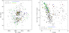 |
Fig. 1. Left: spatial distribution of likely NGC 2264 members with simultaneous lightcurves, highlighting those undergoing simultaneous X-ray+optical and/or X-ray+mIR flaring. X-symbols: all Chandra sources in the “simultaneous” FOVs. Circles: Chandra+CoRoT sources (with unique identifications). Squares: Chandra+Spitzer sources. Green and orange symbols indicate sources with simultaneous X-ray+optical and X-ray+mIR flaring, respectively. Blue crosses indicate stars with a well observed X-ray flare having no counterpart in other available bands (Sect. 6.3 and Appendix D). Note the smaller spatial coverage, but better completeness with respect to the X-ray sources, of the mIR sample with respect to the optical one. Right: same as above in the log LX vs. J-magnitude plane, showing the deeper coverage of mIR data and the tendency of flares to be detected on the stars with higher average X-ray luminosity. |
3. Flare detection and sample definition
Magnetic flares are most easily detected in the soft X-ray band, where the gradual phase, corresponding to the cooling of hot thermal plasma confined in coronal structures, is commonly and easily observed with a large contrast with respect to the “quiescent” coronal emission. We thus started our search for flares from the Chandra X-ray lightcurves and then inspected the simultaneous CoRoT and Spitzer lightcurves in order to identify optical and mIR counterparts. To simplify the detection of the X-ray flares, and their ensuing spectral characterization, we made use of a lightcurve segmentation algorithm developed by ourselves, and already used on several occasions (Wolk et al. 2005; Preibisch et al. 2005; Caramazza et al. 2007; Albacete Colombo et al. 2007). Briefly, our method provides a representation of X-ray lightcurves by using temporal segments during which the photon count-rate is constant or, more precisely, compatible with being constant at a given confidence level. The algorithm is based heavily on the Bayesian Blocks algorithm introduced by Scargle (1998) in that it proceeds by dividing lightcurves at their most likely “break-point” and recursively repeating the process on the resulting segments until the significance of the break-points fall below a set threshold,  . The differences with respect to Scargle (1998) are: (i) we use a maximum likelihood approach in place of a Bayesian one, (ii) significance thresholds for the segmentation process are established via Monte Carlo simulations of constant count-rate sources, (iii) at each of the recursive steps we attempt to fragment the lightcurve by testing two-segment models (with one break-point), as well as three-segment models (with two break-points), (iv) we are able to set the minimum number of photons that the resulting time-segments will include,
  . The last two characteristics are particularly useful for our goals. A three-segment model is indeed more sensitive for detecting impulsive variability (such as flares) than a two-segment model. Moreover, in order to follow the plasma evolution during flares, we need to perform a spectral analysis of the X-ray emission, which requires a minimum number of photons in each segment.
We first computed the segments with a 95% confidence threshold and setting the minimum number of photons per segment to 20. These segments were then used to define a criterion for automated detection of flares, as described in Caramazza et al. (2007), and, once detected, to determine their basic properties in as much of an unbiased way as possible. Start and end times, for example, as well as peak X-ray emission fluxes, were defined based on these segments. It should be noted that our flare detection algorithm, tuned to detect events that follow our preconceived idea of flares (i.e. both elevated flux and time-derivative of the flux), produces mostly reasonable results, but is clearly not perfect. All the Chandra X-ray light curves were thus inspected to determine whether other flare-like events had escaped automatic detection and/or had been improperly defined by our algorithm. Several ad hoc choices were made:
Eleven flares were detected with our automated procedures adopting segments with
 (instead of 20) and the default
  . These are for the most part faint flares, defined by a very small number of photons.
We “forced” the detection of nine X-ray flares with an obvious counterpart in the other bands. In these cases the segmented X-ray lightcurves showed a corresponding elevated X-ray flux which, however, did not qualify as a flare according to our automated criterium2 (for the 2nd flare on ACIS # 677, we also lowered the significance threshold for the segmentation). The X-ray properties of three of these where actually considered uncertain and the flares are not included in our main study sample (see below). We also verified that the exclusion of these nine flares from our sample does not change any of the results discussed below.
For 19 automatically detected flares, we adopted a different set of segments to more accurately describe the shape of flares with respect to those used to detect them. Most often (14 cases) the flare was detected using default segments, i.e. (
 ) = (20, 95%), but we define it using segments with as few as one photon/segment
  . The opposite choice was adopted in one case (ACIS # 1018), and altogether different sets were preferred in the four following cases: ACIS # 297 (
 ) = (1, 99%), 405 (1, 93%), 677 (first flare) and 789 (20, 60%)
In eleven more cases the automatic definition of “flaring” intervals was adjusted by hand. Four flares were defined separating two pairs of events, each of which had been detected as single event (on ACIS # 871 and 924). In five other cases we included/excluded segments that appeared related/unrelated to the events (ACIS # 110, 600, 664, 693, and 1000). Finally, in two cases (flares on ACIS # 630 and 713), a flare was found having the rise phase at the end of the 2nd-last Chandra observing intervals and continuing in the last interval, thus also spanning the short 1.24 h gap between the two: we then modified the default flare definition, which by design is limited to one interval, and included all the relevant segments.
In some cases, only the tail of an X-ray flare was detected at the beginning of one of the Chandra observing segments. We looked at the CoRoT and Spitzer data to search for optical/mIR counterparts that might show the onset of the flare before the beginning of the X-ray observation. Eleven such cases were found: in five of the cases (flares on ACIS # 58, 585, 591, 690, and 1018) the optical/mIR counterpart was reasonably well defined and a large fraction of the X-ray flare, assumed to start at or after the onset of the optical/mIR one, was inferred to have actually been observed. We thus decided that the X-ray flares could actually be defined, although with some uncertainty, and we added them to our sample. We discarded the remaining six cases, however, since either too large a fraction of the X-ray flare may not have been observed or the optical/mIR counterpart could not be uniquely defined.
In one case, two X-ray sources with flares were associated with a single CoRoT source, due to the large CoRoT photometric windows: ACIS # 536 had one X-ray flare with a corresponding event in the CoRoT lightcurve, while ACIS # 541 showed three X-ray flares, two of which with a counterpart in the CoRoT lightcurve. Even though the non-flaring CoRoT emission has ambiguous origin, since we are exclusively interested in the flaring emission, we exploited the time coincidence to confidently associate the CoRoT and X-ray events.
In Table 1 we list the 78 X-ray flares in our sample (from 65 stars), all with a simultaneous optical and/or mIR counterpart. The first three columns list the Chandra ACIS source number (from Flaccomio et al., in prep.), the corresponding Mon identifier from Cody et al. (2014), and the Chandra observation id (or ids) during which the flare occurred. In Fig. 2 we show six representative examples of “good quality” X-ray detected flares, while in Appendix B we show the full sample of lightcurves3.
Flares, deduced physical quantities, and host-star properties.
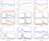 |
Fig. 2. Lightcurves of six of the X-ray flares with optical and/or mIR counterpart discussed in the text. Lightcurves for the full sample can be found in Appendix B, while lightcurves for well defined X-ray flares for which no optical/mIR counterpart was detected are shown in Appendix C. The three panels at the top refer to flares with simultaneous data in all three bands. Within each panel the first two sub-panels, from top to bottom, show the CoRoT lightcurve, normalized to the median of the observed CoRoT flux in the whole exposure (as opposed to the short segment shown), and the Spitzer lightcurve in the IRAC 3.6 μm or 4.5 μm bands (as indicated by the y-axis label and in orange and red, respectively). For both panels a gray line indicate the polynomial intended to represent the non-flaring emission (see text). The ACIS source number of the star and its mIR class are given at the top-left and top-right corners, respectively. The third and fourth panels show the same CoRoT and Spitzer lightcurves, this time subtracted by the non-flaring emission (units given in the right-hand y-axis). The areas shaded in gray indicate our choice for the definition of the optical and mIR flares. The same two panels show the simultaneous Chandra X-ray lightcurve, both binned (black dots with error bars), and using the piece-wise representation discussed in the text (black broken line). Units are shown on the left-hand y-axis. The temporal extension of the X-ray flare, according to our definition, is indicated by a magenta horizontal bar at the top of each panel. The three panels at the bottom show three more X-ray flares with simultaneous CoRoT data, but lacking Spitzer data. |
Out of our 78 X-ray flares, 58 (from 46 stars) have a CoRoT counterpart, 32 (from 30 stars) a Spitzer counterpart, and 13 (from 12 stars) have both. These flare samples are obviously affected by selection biases, which might be even more severe than those affecting the samples of stars simultaneously observed in two or three bands (see Sect. 2), and which ought to be taken into account when interpreting our results. Figure 1 shows the distribution of the flaring stars in our samples in sky coordinates and in the time-averaged LX vs. J-band magnitudes scatter plot. Stars on which we detected simultaneous X-ray/optical flares are systematically brighter in X-rays than the stars with just simultaneous X-ray and optical lightcurves (median log LX = 30.4 erg s−1 vs. 30.0 erg s−1), which are in turn systematically brighter than the general population of X-ray sources (median log LX = 29.6 erg s−1). The same is true for stars with simultaneous X-ray and mIR flares with respect to the stars with just simultaneous X-ray and mIR lightcurves, (median log LX = 30.3 erg s−1 vs. 29.5 erg s−1). This latter sample, even if limited to two small regions in the sky seems, however, to be quite representative of the full X-ray population in those regions in terms of X-ray luminosities. However, because of the chosen Spitzer pointing toward active star forming regions, all mIR data are biased toward stars in early evolutionary stages (Class II and Class I) and with larger than average extinction.
We inspected the CoRoT and Spitzer lightcurves to try to identify flares independently from the X-ray lightcurves. This is not straightforward as faint flares are harder to identify against the strong quiescent and, most often, highly variable optical or mIR emission. Searching the CoRoT lightcurves, we only found one convincing flare-like feature with no corresponding X-ray counterpart. In another 5 stars, we detected suggestive low-significance features which might actually be associated with a low-significance X-ray feature. We found only one convincing Spitzer-only flare which, however, occurred while the relative X-ray source was extremely faint (just one detected photon in the last 67 ks long observing segment, and moreover coincident in time with the mIR flare). We conclude that our data indicate that while X-ray only flares are rather common (see Sect. 6.3), optical- and/or mIR-only flares are rare, if at all present.
4. Flare characterization
In this section we describe, separately for the three spectral bands, how we characterized our flares. For the scope of the present paper, we will focus solely on time-integrated emitted energy and on peak flare luminosity. The estimates of these two quantities in the three bands will be discussed and compared in the following section.
4.1. X-ray data
As described in the previous section, each X-ray flare is defined as a group of one or more consecutive “maximum likelihood” (ML) time intervals. In order to estimate the luminosity at the flare peak, LX, pk, and the total emitted energy, EX, both in the 0.5–8.0 keV band, we first evaluated absorption-corrected X-ray luminosities for each of the individual intervals, LX, i. The maximum of these values was then taken as LX, pk, while EX was taken as the sum of LX, i × ΔTi, where the ΔTi indicates the duration of the segments in seconds.
In most cases, the LX, i were estimated through spectral fitting of the X-ray spectra extracted for each segment. The spectral fits were performed using the XSPEC package, modeling the flaring emission with the APEC isothermal plasma emission model, subject to absorption from intervening interstellar and circumstellar material (TBABS). The non-flaring emission, also contributing to the flux in each of the intervals but of no interest for our purposes, was taken into account by adding a suitable spectral model (see below) with no free parameters. The absorption-corrected fluxes of the flaring components were then converted to luminosities adopting a distance of 760 pc.
In many cases the spectra of individual segments are defined by a small number of photons, resulting in large uncertainties on the best-fit fluxes, mostly due to uncertainties on the absorbing column density, NH. Since the NH does not generally vary during flares4, we significantly reduced the uncertainties by fixing NH to the best-fit, time-averaged, value obtained by Flaccomio et al. (in prep.) fitting the combined spectrum from all the available Chandra data with a physically meaningful model.
The spectral model for the quiescent or characteristic X-ray emission (Wolk et al. 2005) during each flare was determined, for each source, from a distinct set of ML time intervals defining the source “characteristic” emission, as defined in Wolk et al. (2005) and Caramazza et al. (2007). By excluding all flares or other times of elevated flux, the X-ray emission in these sets of ML intervals well approximates the pre- and post-flare emission. A spectral model representative of the characteristic X-ray emission was obtained by simultaneously fitting the spectra extracted from these segments with a model with a large number of free parameters5, with little regard for their physical meaning. Although parameters were most often not constrained, these models served our sole intention of obtaining an accurate representation of the observed out-of-flare spectrum.
In a minority of cases, the spectra of some, or all, of the ML intervals defining a flare contained too few photons to perform a meaningful spectral fit. In these cases we estimated the energy flux from the absorbed photon flux for the segment (in ph s−1 cm−2), subtracted by the characteristic photon flux, the time average for all time intervals defining the characteristic emission level (see above). The thus corrected photon flux is finally converted to absorption-corrected energy flux multiplying it by a conversion factor, taken as the ratio between the time-averaged absorption corrected energy-flux of the source (from spectral fittings in Flaccomio et al., in prep.) to its observed time-averaged photon-flux. This approach is equivalent to approximating the X-ray spectrum during a given ML segment with the time-averaged one. Thus neglecting the increase in plasma temperature that usually characterizes flaring emission, we generally obtain slightly smaller fluxes with respect to those obtained by spectral fitting. The difference is, however, small and negligible with respect to all other sources of uncertainties6.
Finally, for the flare on ACIS # 713, one of the two including the observing gap between the two last observing segments, discussed in Sect. 3, we approximately accounted for the missing observing time, by multiplying EX, as determined above, by the ratio between the duration of the flare and the observed time (1.50). No correction was considered for the other similar case since the observed fraction of the flare is, in this case, significantly longer than the gap.
4.2. CoRoT data
The optical counterparts to the X-ray flares, in the CoRoT lightcurves, were most often harder to define with respect to the X-ray events. We followed an iterative approach. For each flare, we started by examining the CoRoT lightcurve in the same time interval spanned by the Chandra observation segment during which the flare was detected7. In order to account for the large non-flaring variability of our stars we then subtracted the “quiescent” emission, determined through a polynomial fit to the CoRoT lightcurve in the considered time interval. The order of the polynomial was initially chosen as 3 or 5 for time segments shorter and longer than 0.4 days, respectively. In order to reduce the influence of positive deviations, such as flares, we settled, after some experimentation, on a robust asymmetric sigma-clipping procedure8. We then inspected both the original CoRoT lightcurve and the continuum-subtracted one to visually search for the optical counterparts of the X-ray flare. If unsuccessful, we also tried to rebin the CoRoT lightcurve (in cases of low signal) and to vary the standard filtering for removal of bad data-points9. Once the presence of an optical flare was determined, we refined the fit of the out-of-flare lightcurve by excluding the time interval during which the flare was observed, adjusting the degree of the polynomial, and, in a small number of cases in which the fit was unsatisfactory, limiting the fitted temporal interval. We then refined the choice of binning and light-curve filtering (see above) that resulted in a “better looking” flare in the continuum-subtracted lightcurve. We finally defined ad-hoc start and end times and preceded to estimate the time-integrated and peak fluxes, both in instrumental units.
The conversion of instrumental fluxes to intrinsic source luminosities (and time-integrated fluxes to total emitted energies) is not straightforward, especially for a wide-band telescope such as CoRoT, moreover not optimized for absolute photometry. Appendix A illustrates how we proceeded in order to derive the extinction law for the CoRoT band and conversion factors from instrumental to bolometric fluxes10. Both of these derivations depend critically on the source spectrum. Lacking precise information, we considered two alternative shapes for the optical spectrum of our flares: a stellar photospheric spectrum and a black body. In both cases the extinction law and conversion factor depend on the source temperature, while, for stellar-like spectra, the dependence on surface gravity turns out to be negligible. In the following we will mainly assume, for our flares, a black body spectrum with T = 104 K. As we will indicate, however, our main results will not depend significantly on this assumption. All absorption-corrected fluxes were finally converted to luminosities multiplying by 4πd2, with d = 760 pc.
4.3. Spitzer data
The analysis of the Spitzer lightcurves proceeded in much the same way as that of the CoRoT ones. Unlike the CoRoT lightcurves, the Spitzer staring-mode data does not extend beyond the Chandra observing intervals, and we therefore could not search for the rise phase of mIR flares before the beginning of the Chandra observations. Like for the CoRoT case, we convert the observed fluxes, in this case provided in physical units (mJy), to bolometric luminosities (in erg s−1 cm−2). The conversion factor for the 3.6 μm and 4.5 μm IRAC bands, function of the source spectrum and of the intervening extinction, were derived for photospheric models and black body spectra, in the same way described in Appendix A for the CoRoT band. We will initially assume a black body spectrum with T = 104 K, as we did for the optical quantities. In doing so we are assuming that the mIR emission originates from the same spectrum as the optical emission detected by CoRoT. In the following we will, however, test this initial assumption.
5. Results
In Table 1 we present, for our sample of X-ray detected flares, estimates for the X-ray energy and peak flux in the 0.5–8 keV band, and for the “bolometric” energies and peak fluxes from the optical and mIR lightcurves, assuming a T = 104 K black body spectrum.
The X-ray quantities are corrected for absorption. The listed optical and IR quantities are instead not corrected for extinction, which is small in most cases. In the following we will, however, use extinction-corrected energies and luminosities. In Table 1 we report two independent estimates of intervening material: AV, based on spectral types and source photometry from the literature, also listed in Table 1, and the column density of neutral hydrogen NH, estimated by Flaccomio et al. (in prep.) fitting the time-averaged X-ray source spectra with absorbed thermal plasma emission models (with either one or two components). Both estimates suffer from considerable uncertainties. In adopting an extinction correction for our flare peak luminosities and total energies, we considered both estimates. We find that the X-ray values, converted to an optical extinction through the relation AV = NH/2.1 × 1021 (Zhu et al. 2017) produces slightly more significant correlations between the optical and X-ray measurements (see below). This may be attributed to two facts: (i) the estimates of NH are available for more sources/flares, and (ii) the NH is estimated from data which is, on average, much more simultaneous with the flares with respect to the AV values11. In the following we will thus correct our optical and mIR quantities using the X-ray derived extinction values, but will note whether our results depend on this choice. We made an exception for the optical+mIR flare on source ACIS # 405, for which a large discrepancy is found between optical and X-ray absorption estimates: we adopt the optical estimate and cosider all energies and peak luminosities as highly uncertain12, thus effectively excluding the flare from our main sample (see below).
In addition to the quantities described above, Table 1 also list data from the literature for the flaring stars: mIR class (Sung et al. 2009; Cody et al. 2014)13, Hα equivalent widths (Dahm & Simon 2005; Rebull et al. 2002), spectral types (Walker 1956; Makidon et al. 2004; Dahm & Simon 2005), V, R, I magnitudes (Lamm et al. 2004; Sung et al. 2008), CoRoT light curve type (Cody et al. 2014; Venuti et al. 2017) and rotational periods (Lamm et al. 2004; Venuti et al. 2017).
5.1. Optical and X-ray emission
In Fig. 3 we show the relation between optical bolometric and X-ray emitted energies and peak fluxes. We indicate with different colors flares from stars with and without indication of circumstellar disks. Empty symbols indicate flares for which the estimates of either of the plotted quantities were deemed highly uncertain.
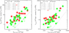 |
Fig. 3. Left: total “bolometric” emitted energy, Eopt, estimated from the CoRoT lightcurves (see text) vs. energy emitted in the 0.5–8.0 keV band, EX. Green and red circles indicate flares from Class III and Class II stars, respectively. Filled circles refer to the flares in our main samples, empty ones to flares with particularly uncertain estimates. The dashed lines shows the unit relation, while the solid lines show the results of six different linear fits (in the log–log plane) performed with different methods, and whose parameters are shown in the upper part of the panel along with the 1σ dispersion of residuals. The fitting methods are: (1) Ordinary Least Squares Y vs. X, (2) Ordinary Least Squares X vs. Y, (3) Ordinary Least Squares Bisector, (4) Orthogonal Reduced Major Axis, (5) Reduced Major-Axis, (6) Mean ordinary Least Squares. Right: same as the plot on the left, but for peak luminosities instead of energies. |
A clear correlation is observed for both the emitted energies and for peak luminosities. The optical values are almost always significantly larger than the soft X-ray quantities. We fit the logarithms of the plotted quantities (filled symbols only) with straight lines using six different methods as provided by the SIXLIN routine in the ASTROLIB IDL library. The results for the 46 flares depicted as solid symbols are shown within each panel, along with the 1σ dispersion computed from the corresponding quantiles of the distribution of y-axis residuals. For emitted energies we obtain  with aE ∼ 6.3 and bE ranging between 2/3 and 1. For peak luminosities we obtain
  with aL ranging from 5.2 to 14.7 and bL between 0.6 and 1.0. In spite of a couple of discrepant points, lying in both panels close to the unity relation (the gray dotted lines), the 1σ scatter about the best-fit relations are as low as 0.27 dex and 0.22 dex for energies and luminosities, respectively.
We note that a different assumption for the optical flare spectrum, such as assuming a photospheric spectrum instead of a black body, or a different temperature, would imply an almost rigid shift in the y-axis (since the effect of source-dependent extinction is small). The amount of this shift can be read from Fig. A.3 and is < 0.3 dex, toward lower values, for 4000 < T(or Teff) < 10 000 K. An unaccounted-for source-dependent T (or Teff), surely a likely occurrence, would contribute to the observed scatter. As for the choice of extinction, had we adopted the AV values from Table 1 to correct the optical energies and luminosities, the correlations would be similar to the ones shown in Fig. 3, but would include only 35 flares (instead of 46) and would have slightly larger scatters, both for flare energies (average for the six regressions: 0.33 dex vs. 0.28 dex) and, even more, for luminosities (average ∼0.38 dex vs. ∼0.25 dex). The coefficients of the correlations would also vary, with aE ∼ 9, bE between 0.7 and 1.2, aL between 9 and 34, and bL between 0.7 and 1.3.
5.2. mIR emission
In Fig. 4 we show the run of the bolometric energies and peak luminosities, as computed from the mIR Spitzer lightcurves (EIR and LIR, pk, either from the 3.6 μm or 4.5 μm data) vs. the corresponding X-ray quantities (EX and LX, pk). A correlation between energies may be observed, but it is surely less significant than the optical vs. X-ray correlation. We applied the Spearman’s ρ and Kendall’s τ correlation tests obtaining null probabilities of 3.2 and 2.3%, respectively. Limiting the sample to Class II surces, the correlation becomes more significant (Pnull = 0.01/0.04%). The most striking feature of the plot is, however, the fact that flares from Class II stars appear to have a higher EIR/EX ratio with respect to those from stars without disks. This in confirmed by a Kolmogorov–Smirnov (KS) test which indicates that the likelihood that two samples are drawn from the same population is 0.19% (0.01% if we include the uncertain points plotted as empty symbols). Similar conclusions can be drawn for peak luminosities: the correlation between the two quantities is slightly less significant for the whole sample (Pnull = 5.5/4.4%), but still significant for flares from Class II stars (Pnull = 0.005/0.04%). For LIR/LX the KS test again indicate a significant difference between flares from stars with and without disks, with Pnull = 0.05% (0.004% including uncertain points). Finally, the two flares from Class I sources may have even larger emission in our mIR bands with respect to the Class II (and III) samples.
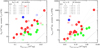 |
Fig. 4. Left: bolometric flare emitted energy, estimated from the Spitzer lightcurves assuming a 104 K black body spectrum, EIR, vs. EX the energy emitted in the 0.5–8.0 keV band. Symbols and lines as in Fig. 3/5, with the addition of blue circles, which indicate flares from Class I sources. Right: same as the plot on the left, but for peak luminosities instead of energies. |
In contrast to the CoRoT instrumental-to-bolometric flux conversion, which is rather insensitive to the incoming spectrum thanks to the CoRoT broad wavelength response, the estimation of bolometric fluxes from the observed mIR fluxes is highly dependent on the assumed spectrum. Assuming a 104 K photospheric spectrum would increase EIR and LIR, pk by ∼25%, while choosing a cooler black body for the optical/mIR flare emission would significantly decrease the estimated bolometric flux, for example by a factor of ∼4 for T = 6000 K. Significant systematic uncertainties and scatter might therefore be introduced by our assumption of similar flaring optical/mIR spectra. If the assumption holds, however, the slopes of the regressions would not be affected. Also substantially unaffected would be the results of the KS test on the difference of EIR/EX and LIR/LX between flares on stars with and without disks. Had we corrected the mIR flare fluxes using the optically derived AV instead of NH the number of available points would have been reduced from 20 to 11, since AV is not available for some of the most absorbed stars, especially those with disks. The correlation tests are in this case inconclusive. The difference in the distributions of EIR/EX and LIR/LX, between stars with and without disks, remains somewhat significant: Pnull=1.83% and 0.23%, for energies and luminosities, respectively (0.66% and 0.40% including uncertain data-points).
We will now investigate the ratio between mIR and optical flare emission. Unfortunately the number of flares with a good characterization of flares in the two bands is small: eight flares, five and three from stars with and without disks, respectively. However, all IR flares in our sample have an X-ray counterpart, and their optical energy and peak luminosity may be approximatively estimated from the correlations shown in Fig. 3. Adopting the “Ordinary Least Squares“ relations, we thus estimate Eopt and Lopt, pk also for flares with no optical counterpart.
In Fig. 5 we use these estimates to plot the EIR/Eopt ratio vs. EX, and LIR, pk/Lopt, pk vs. LX, pk. Circles indicate measured values while squares the ones estimated from the X-ray quantities. No clear correlation is observed. However, it is quite clear that flares on Class II (and, even more, Class I) sources have a significantly larger IR/optical ratio than those on Class III stars.
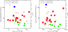 |
Fig. 5. EIR/Eopt vs. EX (left) and LIR, pk/Lopt, pk vs. LX, pk (right). Eopt and Lopt are derived either from the analysis of the CoRoT lightcurves (shown as circles) or estimated from the X-ray quantities and the correlation with the optical ones (squares). The remaining symbols are as in Fig. 4. The vertical scale on the right-hand axes indicate the temperature of the black body spectrum, assumed to be responsible for the emission in the optical and IR bands. The results of KS tests comparing the distributions of the optical/IR ratios for flares from Class II and Class III sources are shown in the upper-left corner, both for the higher quality flares (filled symbols) and for all flares. Note that, at least for the higher quality flares, the null probabilities reported indicate that the distributions are significantly different. |
If the flaring optical and mIR emission, detected with CoRoT and Spitzer, came from the same emitting regions, and thus probed different parts of the same spectrum, and if this spectrum were the same for all flares, the ratio of the Ebol (Lbol, pk) values estimated from the two bands would be a constant. If the spectra were precisely those we have assumed (104 K black bodies), the ratios would be equal to one. The fact that all ratios are larger than one then indicates that the spectra depart from our assumption. The large scatter, moreover, tells us that the spectra are not all the same. If we assume that, for a given flare, the optical and mIR emission comes from the same spectrum and that these are black bodies (or photospheric-like spectra), we can easily relate the optical/IR ratios to the (effective) temperature of the optically/mIR emitting region. The relation depends only very slightly on the IR band adopted to derive EIR and LIR, i.e. 3.6 μm or 4.5 μm. The y-axis on the right-hand side of the two panels in Fig. 5 shows the mean correspondence14.
A KS test shows that well characterized flares from Class II and Class III sources have different distributions of EIR/Eopt, (or of the derived temperatures, Pnull = 0.13%), as well as LIR, pk/Lopt, pk (or of the derived temperatures, Pnull = 0.04%). The significance of these conclusions are not affected by the assumption of a black body vs. photospheric spectra. Flares on Class III stars seem to originate from hotter material with respect to those from Class II (and Class I) sources, and to span a much narrower range of temperatures, especially when considering the temperatures derived from peak luminosities (T = 7000−8000 K). Alternatively, the optical and mIR flares we observe in stars with circumstellar material (Class II and I) might originate from different regions, so that the temperatures we estimated would be meaningless: one can easily envisage a scenario in which the optical flares originate at the feet of the flaring loops (and trace the plasma heating phase) while the mIR flux is dominated by the emission from the inner disk (or envelope), heated or otherwise affected by the optical and X-ray emission of the flare.
5.3. Duration and start times
Measuring the duration of flares from the lightcurves is not always straightforward, especially for faint/low signal events. We here define the flare duration τ, as the ratio between the emitted energy and the peak luminosity. This definition, which corresponds to the decay time for a pure exponential decay, can be easily applied to the three bands. It is, however, subject to biases, most notably from the underestimation of the flare peak luminosities, which is unavoidable with our direct measurement procedure and limited statistics and/or temporal resolution. Durations may thus be systematically overestimated. This bias may be more severe in the X-ray band where the signal-to-noise ratio is the lowest.
In Fig. 6 we compare the duration of flares with simultaneous coverage in the three bands. We observe that X-ray flares are on average longer than both their optical and mIR counterparts, while the optical and mIR flares have similar durations (within a factor of ∼2). No clear difference is observed between flares on stars of different classes.
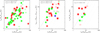 |
Fig. 6. Comparisons between the duration of flares in different bands. The three panels show all three possible comparison between the X-ray, optical, and mIR bands. Duration are defined as described in the text, as the ratio between integrated energy and peak luminosity. Flares plotted as squares are those observed in all three bands. The remaining symbols and colors are as in Figs. 3 and 4. The thick gray diagonal line indicates the unit relation. Thinner lines deviations by factors of 0.5, 2.0, 4.0, and 8.0. The results of KS tests comparing the distributions of the ratios of the two plotted quantities for flares from Class II and Class III sources are shown in the upper-left corner, both for the higher quality flares (filled symbols) and for all flares. The null probabilities reported do not evidence any significant difference. |
We also attempted to estimate the start times of flares in the three bands: however, while in X-rays we can profitably make use of the maximum-likelihood segmentation described in Sect. 3, determining the start time in the CoRoT or Spitzer lightcurves is not straightforward. Whenever reasonable, we have estimated the delay between the onset of an X-ray event and that of the CoRoT/Spitzer one by simple inspection of the lightcurves shown in Appendix B. These estimates are probably good within 0.01 days (∼14 min). Some prominent examples of such delays can be observed for the flares from ACIS sources # 42, # 104, # 677 (first flare), and # 713. Figure 7 shows the distributions of these delays, separately for Class II and Class III stars. The X-ray flares almost invariably trail both the optical and the IR flares, by ∼0.01 days. Observational biases might well affect this result: for example, the X-ray events might be detected with a delay simply because of the limited photon statistics. At face value, however, stars with disks appear to have slightly longer delays, with respect to both the optical and the IR counterpart. In no case, however, are the distributions statistically incompatible with each other. A comparison between the two delays (optical vs. X-ray and mIR vs. X-ray), shows that the two are equal or within the (significant) uncertainties. This, together with the similarity in duration, may point toward a common origin of the optical and mIR flares.
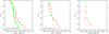 |
Fig. 7. Distributions of time delays between the flare start times in the optical band vs. X-rays (left panel), IR vs. X-rays (center), and optical vs. IR bands (right). Distributions for flares on Class II and Class III stars are plotted separately in each panel in red and green, respectively. The results of KS tests comparing the two distributions are shown in the lower-left corner, indicating in all cases that the distributions are not significantly different. |
6. Discussion
Our characterization of flares in the X-ray, optical and mIR bands is plagued by a significant number of uncertainties. Some are mostly stochastic, e.g. those related to the uncertain definition of the shape of the underlying emission (from the corona, photosphere, or the inner disk), the choice of the flare start and end times, and the absorption correction. Some may be systematic, such as those related to the uncertain nature of the flare optical/IR spectrum and the conversion between observed and physical quantities. In spite of these large and hard to quantify uncertainties, we are able to draw several conclusion.
6.1. Energetics
Much more energy is emitted in the optical band with respect to the soft X-ray band. This is consistent with previous finding for solar and stellar flares (Fletcher et al. 2011). Here we are able to derive a correlation spanning about two orders of magnitude, for flares that are several orders of magnitude more energetic than the ones observed on the Sun. The correlation is rather tight and consistent with the idea that the optical emission traces the plasma heating process, and that a fraction of this energy is then radiated away by the plasma-filled loops in the soft X-ray band. The fact that optical flares are almost always shorter than their X-ray counterparts, and that they also usually start ∼15 min earlier, agrees with this picture. Moreover, although a detailed analysis of the lightcurves of the brightest of our flares is beyond the scope of the present work, we notice that some flares seem to show the Neupert effect (Neupert 1968) in that the time integral of the optical emission appears to track the soft X-ray lightcurve (e.g. flare on source # 789 in Fig. 2).
Since the presence of a circumstellar disk seems irrelevant for the optical/X-ray correlation, either the coronal loops involved are unaffected by disks (and accretion) or the modifications are not relevant for the heating of the plasma in the flaring structures and for its radiative cooling. The slope of the log Eopt vs. log EX correlation is such that, as flares become more powerful, either more of the total energy is converted to X-ray radiation, or a smaller fraction is emitted in the optical band, or both.
The correlation between peak X-ray and optical luminosities is even tighter than for total energies. Since optical flares are shorter, their peak luminosity, Lopt, pk is even larger with respect to the X-ray peak luminosity LX, pk than Eopt is with respect to EX. The slope of the correlation, however, appears similar. Again the presence of a circumstellar disk does not appear to make a difference.
How does the correlation we find compare with what is observed for Solar flares? Woods et al. (2006) find that the total irradiance of four bright solar flares (≳1032 erg s−1) is ∼105 times the energy in the GOES band (0.1–0.8 nm), which translates to 50–80 times the soft X-ray energy in our 0.5–8.0 keV band, assuming a reasonable range of average flaring plasma temperatures between 2 and 5 keV. Since about 1/2 of the total energy is found to be in the near UV+optical+IR bands, we infer that, for flares with Eopt ∼ 1032 erg s−1, Eopt = (25 − 40)×EX(0.5 − 8 keV). Excluding the two linear fits with the most extreme slopes in our Fig. 3, the Eopt/EX values we extrapolate for Eopt ∼ 1032 erg s−1 are, for the four remaining linear fits, 55, 110, 59, and 45. We consider these values compatible with what inferred for the bright solar flares of Woods et al. (2006), given the significant uncertainties of both estimates.
6.2. Origin of the optical/mIR flares
A couple of flares in Fig. 3 appear to lie below the general correlations so that their optical and X-ray energies (and peak luminosities) are similar. This may, again, be consistent with the idea that the optical emission originates at the feet of the flaring loops, on the chromosphere or photosphere, while X-rays are emitted by extended coronal loops. Low optical-emission flares might occur close to the stellar limb so that, while the X-ray loops are fully in view, the feet of the loops are either only partly visible, or obscured by a large amount of intervening material, or the viewing angle reduces the fraction of the optical emission that reaches the observer, for example because of a projection effect or limb darkening. Among these optically faint flares, two, albeit with poor-quality estimates, have mIR counterparts (ACIS # 424 and # 747) and both are Class III stars. Since the optical and mIR emission in Class III stars are likely to share the same physical origin (Sect. 6.4) and the mIR bands are much less affected by extinction with respect to the CoRoT band, these flares allow us to test the extinction hypothesis. Of the flares from Class III sources, they are the ones with highest ratio between mIR and optical emission, thus providing support for this picture.
Further considerations on the observed scatter in the optical vs. X-ray relations (Fig. 3) may constrain the nature of the optically emitting regions. Are they optically thick, as we have implicitly assumed approximating their spectrum with a black body or a photospheric emission model? Or are they optically thin? In both cases we might expect to see a signature in the residuals of optical vs. X-ray correlations. If the emission from the loop feet is optically thin, we should expect no effect in the residuals due to the viewing geometry of the flaring loop: when we see the feet of the loop we should presumably also see the X-ray emitting loop and both emissions should be unattenuated. If, on the other hand, the emission from the feet of the loop is optically thick, and assuming a slab-like geometry, we would expect that the observed emission is attenuated due to the reduced projected area of the emitting region, by a factor cos θ, where θ is the angle between the line of sight and the normal to the emitting surface. Moreover, making the rough assumption that the thermal structure of the emitting region is similar to that of an unperturbed stellar photosphere, we would expect a further attenuation due to limb darkening. Figure 8 shows the cumulative distribution of residuals from the Lopt, pk vs. LX, pk relation in the right-hand panel of Fig. 3. Solid black distributions refer to the residuals according to each of the six linear regressions performed in the log–log plane (a very similar plot is obtained for the Eopt vs. EX relation). If we assume that the angle θ is uniformly distributed between 0 and π/2 we can easily derive the distribution of the expected attenuations due to both projection effects and limb darkening15. These are plotted as thick dashed lines, one for the projection cos θ effect only, and the other also taking into account limb darkening. Both are shifted along the x-axis so to have zero median value. We see that the observed scatter around the best fit regression line is actually smaller than that predicted by these attenuation models. This is quite striking, since we can identify several sources of stochastic uncertainties in our estimates of Lopt, pk and LX, pk (or Eopt and EX), which surely contribute significantly to the observed scatter (an accurate analysis of uncertainties is, however, not straightforward). The intrinsic scatter in the optical vs. X-ray relations is thus likely much smaller than we predict assuming optically thick emission and an uniform spatial distribution of the emitting spots on the stellar disk. We take this as a suggestion that the flare emission in the CoRoT band is optically thin.
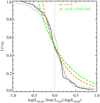 |
Fig. 8. Solid black lines: cumulative distributions of residuals in the linear fits to the log Lopt, pk vs. log LX, pk scatter plot. Each line refers to one of the six linear fits shown in Fig. 3. Dashed orange line: predicted distributions assuming the optical peak luminosity is perfectly correlated to the X-ray peak luminosity and that the observed optical flux, from an optically thick slab-like region, is attenuated by projection effects (see text). Dashed green line: same as above with an additional attenuation due to limb darkening. The fact that the observed scatter is smaller than predicted by these assumption, even ignoring measurement uncertainties and flare-to-flare variations, indicates that the assumptions on the optical emitting regions are not correct. |
6.3. Optically undetected flares
We now discuss the X-ray flares for which no optical/mIR counterpart could be detected. One obvious physical scenario in which this could happen is when we observe the extended X-ray emitting loops while the optically bright foot-points fall behind the stellar limb. The occurrence rate of such a geometry depends on the height of the X-ray emitting loops. We will thus try to relate the statistics of optically detected/undetected flares with the average extension of the flaring magnetic loops. Although this is not straightforward for a number of reasons (e.g., we must try to account for band-dependent sensitivity in the detection of flares, as well as for false positives and negatives) we feel that the effort is justified since this could well be one of the very few available handles on the extension of coronae on PMS stars.
In addition to our main sample of 78 X-ray flares with reasonably defined optical and/or mIR counterparts, the main focus of this paper, our automatic detection algorithm for the detection of X-ray flares, with default parameters, also singles out 97 more X-ray events16. For a fraction of these, a likely optical/mIR counterpart is actually found but we assessed that the optical and/or mIR and/or X-ray flare could not be satisfactorily defined, and thus included in our main sample, for one of the following reasons: (i) the X-ray event is detected at the beginning of the Chandra observing segments and the likely optical/mIR counterpart significantly precedes the beginning of X-ray observation, implying that we are not observing a significant fraction of the X-ray flare; (ii) the X-ray event is at the very end of the Chandra observing segments, we see no hint of a decay phase, and the X-ray event could not be defined; (iii) the X-ray event is contained within the Chandra observing segment and some likely associated optical/mIR feature is observed, but cannot be easily isolated. Appendix C shows the 24 flares (from 21 stars) that fall into one of the above categories and which, in the following, we will consider as detected in the optical/mIR band, alongside the flares in our main sample. For consistency with the present analysis, however, we will only consider the subset of flares in our main sample that were detected with our default procedure (Sect. 3): focusing, from now on, on flares with optical (CoRoT) counterparts, this reduces our main sample to 49 flares, to which we must add 18 of the 24 flares from the above selection of events with likely optical counterparts. We thus have a total of 67 X-ray flares with optical counterparts. These must be compared to the total of 62 detected X-ray events with CoRoT data and no significant hint of an optical counterpart. Our starting estimate for the fraction of X-ray flares with no optical counterpart, fX, noOpt, is thus 62/(62 + 67) = 48.1%.
As already indicated, assuming that optically undetected X-ray flares are due to flaring loops with feet behind the stellar limb, fX, noOpt can constrain the average hight of flaring loops, hf, relative to the stellar radius. Indeed, if hf ≫ R⋆ the fraction would approach 1/2. If, on the other hand, hf ≪ R⋆ the fraction would be close to zero. We derive a relation between fX, noOpt and hf through a simple geometrical zero-order approximation of flaring loops, i.e. taking them as 1D straight segments, of height hf, extending radially from the stellar surface. We assume that optical flares originate from the feet of these segments and are detected anytime these latter are in view, i.e. not behind the stellar limb. X-ray flares are instead assumed to be detected whenever any part of the segment is in view. With these assumptions, and assuming flares are uniformly distributed on the stellar surfaces, we can estimate for a given value of hf, the fraction of flares for which we would detect the X-ray emission but not the optical counterpart, i.e. fX, noOpt. We perform this estimate adopting straightforward Monte Carlo methods for a range of hf values, thus deriving the relation between average fX, noOpt and hf.
We finally obtain that the observed fX, noOpt = 62/(62 + 67), corresponds to a nominal hf = 1.65R⋆, while the 1σ uncertainty range, assuming a binomial distribution for the number of optically undetected X-ray flares is [0.56,∞]R⋆, unconstrained in the upper limit. Two significant issues, however, are likely to artificially increase our estimate of fX, noOpt (and thus hf). First, while close to 100% of the events we identify as X-ray flares with optical counterparts will indeed be coronal flares (because of the temporal coincidence in the two bands), some of the X-ray-only events, might actually not be bona-fide flares. This particularly applies to faint X-ray events detected at the beginning or at the end of the Chandra observing segments and whose duration cannot be determined. For faint X-ray events contained within one of the observing segments, the short duration provides some confirmation of the flare-like nature of the event. Secondly, our X-ray flares with no optical counterpart appear to be significantly fainter in X-rays than those with optical counterparts, with median EX and LX, pk lower by a factor of 1.9 and 2.5, respectively. The correlations between optical and X-ray flare properties imply that, if the optical counterparts to these X-ray flares were observed, they would be fainter and some might fall below our detection sensitivity.
In order to reduce the two aforementioned biases, both leading to an overestimation of the typical loop height, we take two measures: (i) we only consider X-ray flares whose peak is fully contained within its Chandra observing segments (i.e. for which we observe both the rise and at least the beginning of the decay phase) and, (ii) we consider subsamples of bright X-ray flares, with EX and/or LX, pk above set thresholds. Taking the first measure, our sample is reduced to 45 optically detected and 25 optically undetected flares (lightcurves show in Appendix D along with those for seven more similar flares with missing mIR counterpart). With fX, noOpt = 35.7%, our best estimate for hf is 0.20R⋆, with a 90% confidence upper limit of 0.51R⋆. We then also applied our second bias-mitigation measure by considering flare subsamples with the following conditions: (1) LX, pk > 4 × 1030, (2) EX > 3 × 1034, (3) LX, pk > 3 × 1030 and EX > 3 × 1034 and, (4) LX, pk > 6 × 1030 and EX > 4 × 1034. This results in lower estimates for fX, noOpt (19–31%) and stronger constrains on hf, with best-guess estimates ranging from 0.03 to 0.11R⋆ and 90% upper confidence intervals always lower than 0.29R⋆ (lower than 0.09R⋆ for the most constraining sub-sample, #4). We note, however, that in our physical scenario, the X-ray emitting loops of flares with no optical counterpart might be partly hidden by the stellar limb, so that the observable X-ray emission would be reduced. This implies that, in order to properly determine the optical detection frequency of a complete sample of flares, we should not apply the same cut on LX, pk (and/or EX) for optically detected and undetected flares. Using our simplified physical model and our Monte Carlo simulations, we estimate that that the average fraction of the X-ray emitting loop that is visible and contributes to the observed emission depends on hf, ranging from a minimum of 2/3 for the shortest loops to 1.0 for infinitely long ones. Making the reasonable assumption that the (time-averaged) 0.5–8.0 keV emission from the flaring loop is distributed quite uniformly along the height of the loop (cf. Fig. 8 of Reale et al. 2018, and associated on-line animation), we thus repeat the above analysis reducing the thresholds on LX, pk and EX for the optically undetected flares to 2/3 those adopted for the optically detected ones. By thus increasing the number of optically undetected flares in our sample, our estimate for the average loop length increases: our most-likely values for hf range between 0.10 and 0.21R⋆ and the 90% confidence upper estimate remains always lower than 0.64R⋆ (< 0.37R⋆ for subset #4).
We conclude that, although uncertainties are large, the average flaring magnetic loops are rather compact with respect to the stellar dimensions. This is consistent with the results of Flaccomio et al. (2005) on the rotational modulation of coronal emission in the COUP dataset but, of course, does not preclude the existence of rare extremely long flaring loops (Favata et al. 2005; Reale et al. 2018).
6.4. mIR flare emission and physical scenarios
The most striking result of our investigation is possibly the very large mIR emission we observe from our flares and, more specifically, from those occuring in stars with circumstellar disks and envelopes. Stars with no evidence of circumstellar disks, on the other hand, have significantly fainter mIR flares: their mIR and optical emission levels are, moreover, compatible with a single physical origin, most likely emission at the feet of the flaring loops. If this is the case we estimate the temperatures of the emitting region to be in the 7000–8000 K range (assuming black body emission spectra, 6000–7000 K in case of photospheric spectra). We have, however, obtained indications that the emission is optically thin (Sect. 6.1), making our assumptions for the optical/IR spectra unlikely to be fully accurate.
It is tempting to assume that the optical to IR flux and energy ratios that we observe for Class III stars are actually representative of the loop feet for all flares. In this interpretation, the “excess” IR emission observed for flares in Class II stars may be attributed to the heating of circumstellar disks, possibly the inner regions, due to the illumination from optical and X-ray flare emission. This effect may be particularly prominent for the two flares from Class I YSOs, for which heating of the envelope or the different properties of the disks might explain the large IR excesses.
This scenario is plausible since, (i) the dust grains in the inner disk, largely responsible for the mIR emission, are known to be heated by the stellar radiation and, (ii) the cooling time of these dust grains, following the absorption of optical or X-ray photons, should be short when compared to the duration of our flares (Bocchio et al. 2013).
6.5. Temperature of the optically emitting regions
As discussed in the previous section, the ratio between optical and mIR quantities should give us, at least for Class III stars, an indication of the temperature of the optically emitting region. As can be read from Fig. 5 we almost invariably obtain somewhat lower temperatures from the ratio of integrated energies, which might be interpreted as a time-averaged value, than from those of peak luminosities (with the single exception of a flare for which the optical values are indirectly obtained from the X-ray data). The difference between “average” temperatures vs. temperatures at the flare peak might be interpreted as indication that the emitting region cools down during the decay phase. Also, this appears consistent with what inferred from the spectral analysis of moderate/large flares on M dwarfs (Kowalski et al. 2016) for which the flux longword of λ > 4000 Å shows two black-body-like components, one at 1.0−1.2 × 10⁴ K and the other at ∼5000 K, with this latter decaying on a longer time scale with respect to the hot component. In the two-ribbon flare scenario, the hot black body might originate in newly heated kernels, while the cooler component might be associated with the previously heated ribbons.
6.6. Effect of disks vs. accretion
We have so far discussed the difference between flares in stars with and without circumstellar disks (Class IIs and Class IIIs). We now briefly discuss flares from accreting and non-accreting stars, or classical and weak-line T Tauri stars (CTTS and WTTS), as traced by the Hα equivalent width (EW). However, while we have mIR classifications for all flaring sources, we have Hα data for only a fraction, especially for the more embedded sources. Specifically, we have EW(Hα) values for 61 flares, 78%, of our sample, which reduces to 13/20 (65%) for the flares with good-quality X-ray+mIR lightcurves (20/32, 62.5%, including lower quality X-ray+mIR flares).
The indications of accretion largely overlap with those of disks: taking EW(Hα) = 10 Å as the threshold between CTTS and WTTS, the two classifications “agree” for 87% of our flares (i.e. 19 and 33 flares from CTTS/Class II and WTTS/Class III stars, respectively). For only 8 flares, the two classifications differ: 6 flares (from 5 stars) are from Class II WTTSs and 2 flares (from 1 star) are from a Class III CTTS.
We have checked that, had we separated our sample in CTTS and WTTS instead of Class II and Class III sources, the results discussed above would not change. Most of the significances of correlations and of two-population tests would, however, be reduced. For example, the probability that good quality flares from CTTSs and WTTSs have the same distribution of EIR/Eopt (cf. Fig. 5) is 4.8% vs. 0.13% for Class IIs and Class IIIs. It would be tempting to infer that disks, rather than accretion, are responsible for the systematic difference in EIR/Eopt, but the smaller sample size is probably to blame for most of the reduction in significance.
7. Summary and conclusions
As part of the NGC 2264 CSI project, we have observed a significant sample of young stars in the ∼3 Myr old NGC 2264 star forming region, obtaining an unprecedented set of simultaneous lightcurves in the soft X-rays, optical, and mIR bands. We have here focused on the study of magnetic flares, known to be extremely powerful in PMS stars, with the goals of gaining insights on the physics of these strong events and to assess their impact on the evolution of circumstellar disks and protoplanets. We have here conducted a statistical investigation, mainly constraining and correlating the energetics of a sizable sample of flares in the three bands. A detailed analysis of individual events is left for a later study. We are able to draw a number of novel conclusions, among which:
A clear correlation between the soft X-ray and optical emission is observed. The correlation is such that the ratio between emitted energies in the soft X-ray band and in the optical bands range between ∼1/10 and ∼1/4 for EX between 1034 and 1036 erg s−1. These ratios are significantly lower than what inferred for the most powerful solar flares, with bolometric energies ∼3 dex lower than those of our least powerful flares. The slope of our correlation, however, is roughly consistent with these solar events, pointing toward a common physical mechanism.
The durations of flares in the three bands are generally consistent with the accepted picture for solar-like flares in that X-ray flares are almost invariably longer than optical ones, perhaps indicating that the X-ray emission from the cooling coronal loops always follows the heating and subsequent evaporation of the plasma into these loops, as traced by the optical flares. In many cases, however, the X-ray and optical durations are comparable, indicating either compact loops with short cooling times, or prolonged heating. mIR and optical flares, on the other hand, have comparable durations, suggesting that the two have the same physical origin, possibly the feet of the loops, or (see below) that the mIR emission is due to reprocessing of the optical one.
The mIR flares on stars with disks (and circumstellar envelopes) are significantly more intense with respect to their optical counterparts than they are on stars without disks. At least two possible interpretations are possible: (i) both optical and mIR emission come from the feet of the flaring loops and the spectrum of the emission is much redder for stars with disks, indicating cooler emitting regions; (ii) the feet of flaring loop actually have the same spectra and we are observing mIR excesses due to the response of the inner disks to the optical and X-ray flares. In this latter hypothesis, which we tend to favor, the optical emission from the loop feet could come from a region at 7 − 8 × 10³ K, as inferred from the peak luminosities of flares on diskless stars, while most of the observed mIR flux might be reprocessed emission by the circumstellar material. Interestingly the mIR excesses of flares from Class I stars, with both circumstellar disks and envelopes, are among the strongest.
A more involved line of reasoning also allows us to speculate on the physical nature of the optical source in flares, based on the surprisingly small dispersion in the relation between optical and X-ray emitted energies and peak luminosities (Eopt vs. EX and Lopt, pk vs. EX, pk). Although a rigorous analysis of uncertainties on the two pairs of quantities is not straightforward, given the numerous approximations and assumptions made in the process, it is reasonable to assume that a large fraction of the observed scatter may be attributed to uncertainties. This leaves little room for physical flare-to-flare variability. In particular, assuming as reasonable that the X-ray emission comes from optically thin plasma, we can exclude that the observed optical flares are strongly affected by the location of the flare on the stellar surface with respect to the observer. This probably indicates that the optical source is not too deeply set in the stellar atmosphere as to be strongly obscured when viewed close to the stellar limb, and that it is probably optical thin, so not to be subject to projection or limb-darkening effects. In principle, other scenarios may also be possible, however, such as a spherically symmetric optically thick optical source located high up in the atmosphere.
Finally, we constrain the typical hight of coronal flaring loops from the frequency of detected X-ray flares with no optical counterparts. Under the hypothesis that these events are produced by X-ray bright loops whose optically emitting feet are hidden behind the stellar limb, we estimate that the loops most likely extend up to a small fraction of the stellar radius.
As indicated, comparable energy is released in kinetic form both in CMEs and in the accelerated electron streams.
We, however, discarded, some tentative X-ray flares only found by inspection but whose counterpart at longer wavelengths was either questionable or too difficult to define.
In addition to the maximum likelihood segmentation of the X-ray lightcurves discussed above, the figures also show, for comparison, a more traditional representation with fixed bins, with duration varying on a source-by-source basis. This latter is, however, not used in the following.
In a small number of cases increases in the NH during flares have been reported in the literature, possibly related to the associated Coronal Mass Ejection. We do no find evidence of this phenomenon during the flares analyzed here.
Specifically an absorbed- three-temperature plasma model, TBABS(VAPEC+VAPEC+VAPEC) in XSPEC, with variable abundances for all elements.
For 57 flares spectral fits were available for all of the defining segments. For this sample, the emitted soft X-ray energies estimated from the conversion factors are lower than those from spectral fits by 0.08 dex in the median (±1σ quantiles of the ratio distribution: 0.03 and 0.14 dex). An indistinguishable distribution (same median and quantiles) is found for the ratio of 64 peak X-ray luminosities estimated with both methods.
In some cases, for X-ray flares for which only the decay phase was detected, the rising phase presumably falling before the beginning of the Chandra observing segment, we considered a longer portion of the CoRoT lightcurve, starting a few hours before the beginning of the Chandra lightcurve.
We made use of the ROBUST_POLY_FIT IDL routine contained in the ASTROLIB library. After an initial fit with ROBUST_POLY_FIT we determined the standard deviation of residuals, σ, and excluded outlying points, those with offsets from the best fit curve smaller than −3σ and larger than 1.5σ, and repeated the fit. This simple sigma-clipping procedure was repeated three times.
Each CoRoT datapoint is flagged by the standard pipeline for a number of potential issues (see http://idoc-corotn2-public.ias.u-psud.fr/jsp/doc/DescriptionN2v1.3.pdf) and we have initially adopted the STATUS = 0 condition to filter out all possibly affected data-points. We, however, realized that accepting data flagged for certain conditions can, in several cases, result in more flare-like lightcurves and in a better matches with X-ray data (and/or mIR data, see below). This is possibly because (i) some data-points are flagged for potential issues that do not always affect the quality of the data, at least for our science, and (ii) the impulsive phase of flares appears to spuriously trigger some of the conditions used to set some specific flags. We thus quite often accepted data-points for which the status flags 1, 2, 3, 4, 5, and 8 were set. In one single case, one highly discrepant point in the CoRoT lightcurve of ACIS # 331 was removed, in spite of its status flag being zero, to exclude an obviously spurious peak.
Since for our flares we are only interested in variations of the flux, as opposed to total source fluxes, our conversion from the observed CoRoT units to physical units is not strongly affected by the significant background correction issues discussed by Cody et al. (2014), as long as the background is approximatively constant during the duration of each flare.
NH comes from the X-ray spectrum averaged over all existing Chandra observations. For the vast majority of flares, observed during the 300 ks Chandra observations within the CSI campaign, data from additional exposures, up to 160 ks long, were then included. For AV, however, spectral types and photometry were in all cases obtained years before the events.
The NH would convert into an unphysical AV implying, e.g., (V − I)0 = −1.15 and (R − I)0 = −1.04 for the K3 host star, and a peck optical flare luminosity ∼100 times larger than the stellar bolometric luminosity, in spite of the fact that the CoRoT flux increases by only ∼15%. We do not understand the reason of these discrepancies, but note that the star is significantly accreting, so that the disk material and accretion streams might well play a role in the X-ray absorption.
Four YSOs listed by Sung et al. (2009) as possessing transition disks are here treated as Class II sources.
The difference between the temperatures corresponding to given IR/opt ratio in the two bands is always <2.2%.
We have adopted the limb darkening law for the CoRoT band derived by Claret & Bloemen (2011), adopting Teff = 8000 K, log g = 4.0, Z = 0.0, ξ = 2.0 : I(θ)/I0 = 0.437 + 0.872 cos θ − 0.309(cos θ)2.
Three more X-ray flares from two sources were discarded since the two sources are close-by and basically unresolved stars, severely hindering the attribution of features in both the X-ray and optical lightcurves.
Acknowledgments
We than Robert A. Stern for careful reading of the manuscript and insightful comments that helped improve this work, and Fabio Reale and Cesare Cecchi-Pestellini for useful discussions on the properties of flaring loops and on the effects of flares on circumstellar dusts. E. F., S.S., G.M., and M.G.G. acknowledge financial support from PRIN-INAF 2012, as well as, in a modest measure, from the ASI-INAF agreement n.2017-14.H.O.
References
- Albacete Colombo, J. F., Caramazza, M., Flaccomio, E., Micela, G., & Sciortino, S. 2007, A&A, 474, 495 [NASA ADS] [CrossRef] [EDP Sciences] [Google Scholar]
- Auvergne, M., Bodin, P., Boisnard, L., et al. 2009, A&A, 506, 411 [NASA ADS] [CrossRef] [EDP Sciences] [Google Scholar]
- Bai, X.-N. 2011, ApJ, 739, 50 [NASA ADS] [CrossRef] [Google Scholar]
- Benz, A. O., & Güdel, M. 2010, ARA&A, 48, 241 [NASA ADS] [CrossRef] [Google Scholar]
- Bessell, M. S. 1990, PASP, 102, 1181 [NASA ADS] [CrossRef] [Google Scholar]
- Bocchio, M., Jones, A. P., Verstraete, L., et al. 2013, A&A, 556, A6 [NASA ADS] [CrossRef] [EDP Sciences] [Google Scholar]
- Broos, P. S., Townsley, L. K., Feigelson, E. D., et al. 2010, ApJ, 714, 1582 [NASA ADS] [CrossRef] [Google Scholar]
- Caramazza, M., Flaccomio, E., Micela, G., et al. 2007, A&A, 471, 645 [NASA ADS] [CrossRef] [EDP Sciences] [Google Scholar]
- Claret, A., & Bloemen, S. 2011, A&A, 529, A75 [NASA ADS] [CrossRef] [EDP Sciences] [Google Scholar]
- Cody, A. M., Stauffer, J., Baglin, A., et al. 2014, AJ, 147, 82 [NASA ADS] [CrossRef] [Google Scholar]
- Dahm, S. E. 2008, in The Young Cluster and Star Forming Region NGC 2264, ed. B. Reipurth, Handbook of Star Forming Regions, I, 966 [NASA ADS] [Google Scholar]
- Dahm, S. E., & Simon, T. 2005, AJ, 129, 829 [NASA ADS] [CrossRef] [Google Scholar]
- Damiani, F., & Micela, G. 1995, ApJ, 446, 341 [NASA ADS] [CrossRef] [Google Scholar]
- Damiani, F., Maggio, A., Micela, G., & Sciortino, S. 1997, ApJ, 483, 350 [NASA ADS] [CrossRef] [Google Scholar]
- Emslie, A. G., Dennis, B. R., Holman, G. D., & Hudson, H. S. 2005, J. Geophys. Res., 110, A11103 [NASA ADS] [CrossRef] [Google Scholar]
- Ercolano, B., & Owen, J. E. 2016, MNRAS, 460, 3472 [NASA ADS] [CrossRef] [Google Scholar]
- Favata, F., Flaccomio, E., Reale, F., et al. 2005, ApJS, 160, 469 [NASA ADS] [CrossRef] [Google Scholar]
- Flaccomio, E. 2003, in The Young Globular Cluster Cygnus OB2, Chandra Proposal, 1398 [Google Scholar]
- Flaccomio, E., Damiani, F., Micela, G., et al. 2003, ApJ, 582, 398 [NASA ADS] [CrossRef] [Google Scholar]
- Flaccomio, E., Micela, G., Sciortino, S., et al. 2005, ApJS, 160, 450 [NASA ADS] [CrossRef] [Google Scholar]
- Flaccomio, E., Micela, G., Favata, F., & Alencar, S. P. H. 2010, A&A, 516, L8 [NASA ADS] [CrossRef] [EDP Sciences] [Google Scholar]
- Flaccomio, E., Micela, G., & Sciortino, S. 2012, A&A, 548, A85 [NASA ADS] [CrossRef] [EDP Sciences] [Google Scholar]
- Fletcher, L., Dennis, B. R., Hudson, H. S., et al. 2011, Space Sci. Rev., 159, 19 [NASA ADS] [CrossRef] [Google Scholar]
- Glassgold, A. E., Najita, J., & Igea, J. 1997, ApJ, 480, 344 [NASA ADS] [CrossRef] [Google Scholar]
- Guarcello, M. G., Flaccomio, E., & Micela, G. 2017, A&A, 602, A10 [NASA ADS] [CrossRef] [EDP Sciences] [Google Scholar]
- Kowalski, A. F., Cauzzi, G., & Fletcher, L. 2015, ApJ, 798, 107 [NASA ADS] [CrossRef] [Google Scholar]
- Kowalski, A. F., Mathioudakis, M., Hawley, S. L., et al. 2016, ApJ, 820, 95 [NASA ADS] [CrossRef] [Google Scholar]
- Kurucz, R. 1993, ATLAS9 Stellar Atmosphere Programs and 2 km/s grid. KuruczCD-ROM No. 13 (Cambridge, MA: Smithsonian Astrophysical Observatory), 13, [Google Scholar]
- Lamm, M. H., Bailer-Jones, C. A. L., Mundt, R., Herbst, W., & Scholz, A. 2004, A&A, 417, 557 [NASA ADS] [CrossRef] [EDP Sciences] [Google Scholar]
- López-Santiago, J., Crespo-Chacón, I., Flaccomio, E., et al. 2016, A&A, 590, A7 [NASA ADS] [CrossRef] [EDP Sciences] [Google Scholar]
- Makidon, R. B., Rebull, L. M., Strom, S. E., Adams, M. T., & Patten, B. M. 2004, AJ, 127, 2228 [NASA ADS] [CrossRef] [Google Scholar]
- Mathis, J. S. 1990, ARA&A, 28, 37 [NASA ADS] [CrossRef] [Google Scholar]
- McGinnis, P. T., Alencar, S. H. P., Guimarães, M. M., et al. 2015, A&A, 577, A11 [NASA ADS] [CrossRef] [EDP Sciences] [Google Scholar]
- Morbidelli, A., & Raymond, S. N. 2016, J. Geophys. Res.: Planets, 121, 1962 [NASA ADS] [CrossRef] [Google Scholar]
- Neupert, W. M. 1968, ApJ, 153, L59 [NASA ADS] [CrossRef] [Google Scholar]
- Pascucci, I., & Sterzik, M. 2009, ApJ, 702, 724 [NASA ADS] [CrossRef] [Google Scholar]
- Preibisch, T., McCaughrean, M. J., Grosso, N., et al. 2005, ApJS, 160, 582 [NASA ADS] [CrossRef] [Google Scholar]
- Reale, F., Lopez-Santiago, J., Flaccomio, E., Petralia, A., & Sciortino, S. 2018, ApJ, 856, 51 [NASA ADS] [CrossRef] [Google Scholar]
- Rebull, L. M., Makidon, R. B., Strom, S. E., et al. 2002, AJ, 123, 1528 [NASA ADS] [CrossRef] [Google Scholar]
- Scargle, J. D. 1998, ApJ, 504, 405 [NASA ADS] [CrossRef] [Google Scholar]
- Stauffer, J., Cody, A. M., Baglin, A., et al. 2014, AJ, 147, 83 [NASA ADS] [CrossRef] [Google Scholar]
- Stauffer, J., Cody, A. M., McGinnis, P., et al. 2015, AJ, 149, 130 [NASA ADS] [CrossRef] [Google Scholar]
- Stauffer, J., Cody, A. M., & Rebull, L. 2016, AJ, 151, 60 [NASA ADS] [CrossRef] [Google Scholar]
- Sung, H., Bessell, M. S., Chun, M., Karimov, R., & Ibrahimov, M. 2008, AJ, 135, 441 [NASA ADS] [CrossRef] [Google Scholar]
- Sung, H., Stauffer, J. R., & Bessell, M. S. 2009, AJ, 138, 1116 [NASA ADS] [CrossRef] [Google Scholar]
- Venuti, L., Bouvier, J., Cody, A. M., et al. 2017, A&A, 599, A23 [NASA ADS] [CrossRef] [EDP Sciences] [Google Scholar]
- Walker, M. F. 1956, ApJS, 2, 365 [NASA ADS] [CrossRef] [Google Scholar]
- Weingartner, J. C., & Draine, B. T. 2003, ApJ, 589, 289 [NASA ADS] [CrossRef] [Google Scholar]
- Wolk, S. J., Harnden, Jr., F. R., Flaccomio, E., et al. 2005, ApJS, 160, 423 [NASA ADS] [CrossRef] [Google Scholar]
- Woods, T. N., Kopp, G., & Chamberlin, P. C. 2006, J. Geophys. Res., 111, A10S14 [NASA ADS] [CrossRef] [Google Scholar]
- Zhu, H., Tian, W., Li, A., & Zhang, M. 2017, MNRAS, 471, 3494 [NASA ADS] [CrossRef] [Google Scholar]
Appendix A: CoRoT fluxes
The spectral response of the CoRoT Planer Finder channel (Auvergne et al. 2009) spans a broad wavelength range, from ∼3000 to 11 000 μm. The conversion from instrumental flux to physical units (erg s−1 cm−2) thus depends significantly on the incident source spectrum, which, in turn, depends on the intrinsic spectrum and the intervening extinction. We have derived conversion factors from instrumental fluxes to absorption-corrected source fluxes, adopting the spectral response shown in Fig. 14 of Auvergne et al. (2009), the extinction law of Weingartner & Draine (2003) (R = 3.1), and model source spectra. These latter were either Black Bodies with varying temperatures, or the ATLAS9 stellar atmospheric models provided by Kurucz (1993) as a function of effective temperature, surface gravity, and metallicity. For the flares from our PMS stars, we considered models computed for Solar abundances and four values of log g, between 3.0 and 4.5.
We started by deriving the extinction law for the CoRoT band. This is a function of the spectral parameters (Teff and g for the stellar spectra and T for the black bodies), which we will generically indicate with p in the following.
 (A.1)
(A.1)
where F⋆(λ, p) is the intrinsic source spectrum, A(λ)/AV is the extinction law of Weingartner & Draine (2003) assuming R = AV/E(B − V) = 3.1, and QCoRoT(λ) is the normilized quantum efficiency of the CoRoT Planer Finder camera. Figure A.1 shows the thus derived extinction law for the CoRoT band as a function of spectral parameters, alongside those derived in the same way for the V, Rc, and Ic optical filters. For comparison, the dotted horizontal lines show spectrum-independent approximations, as most commonly adopted, derived from the Mathis (1990) extinction law. Note the small dependence of the extinction laws on gravity for stellar-like spectra, and, at least for the CoRoT extinction law, the non-negligible difference between stellar-like spectra and black bodies.
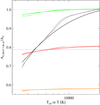 |
Fig. A.1. Extinction laws for the CoRoT band (in black) and for the V, Rc, and Ic optical filters (green, red, and orange, respectively). The thin lines show the variation of A(band)/AV with effective temperature for the stellar-like spectra with log g between 3.0 and 4.5. Thicker lines show the trend of A(band)/AV with temperature for black body spectra. |
Next, we estimated kCoRoT, the conversion factor between CoRoT incident flux, in erg s−1 cm−2, and the flux in instrumental units,  :
:
 (A.2)
(A.2)
where, AV is the extinction suffered by the source. We estimate kCoRoT by comparing, for a suitable sample of stars with known spectral types and extinction, the observed flux in instrumental units with that predicted for our CoRoT sources on the basis of the known stellar spectra (from spectral types), extinction (AV), and photometry (in the R-band). More specifically, we take F⋆(λ, p) as the Kurucz (1993) model with the Teff indicated by the spectral type, AV as derived from the spectral type and observed optical colors, and we set the normalization of the model spectrum so to reproduce the flux measured in the R-band. For each star in the sample we thus estimate one value of kCoRoT:
 (A.3)
(A.3)
where QR(λ) is the R-band filter response function (from Bessell 1990) and  is the measured flux in the R-band, obtained from the R magnitudes as:
 (A.4)
(A.4)
FVega(λ) is here the flux-calibrated model spectrum of Vega provided by Kurucz (1993), whose R magnitude is assumed to be 0.03. If the model spectra, relative parameters, and extinction values were perfectly known, kCoRoT would be the same for all stars in the sample. In order to reduce uncertainties we select a sample of NGC 2264 members observed by CoRoT, with well identified counterpart in the R-band, and with no evidence of disks or accretion (in order to avoid accretion/disk-induced spectral excesses). Figure A.2 shows, as a function of the stellar R magnitude, kCoRoT as estimated for the above sample from Eq. (A.3). Given the uncertainties on the gravity of our stars, we plot, with different colors, values of kCoRoT obtained assuming four different values of log g between 3.0 and 4.5, showing that the effect of surface gravity on our estimates is negligible.
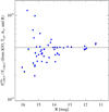 |
Fig. A.2. Ratio between observed CoRoT flux, in instrumental units, and the flux predicted from model spectra vs. observed R magnitudes. The plotted points refer to a subsample of suitable and well characterized NGC 2264 members (see text), and symbols of different colors, largely overlapping with each other, refer to estimates obtained assuming four different values of log g between 3.0 and 4.5. The horizontal line refers to the adopted value, 4.2 × 10¹⁵ erg−1 s−1 cm−2. |
A significant scatter can be noticed at R ≳ 14, up to a factor of ∼2 at the faint end. This can probably be attributed to already identified issues with background subtraction of the CoRoT photometry (see e.g. Cody et al. 2014). Indeed the brighter stars all have low estimated background contributions, and therefore presumably small errors on the background correction, explaining the small scatter in the kCoRoT values. We take kCoRoT as the median of values for R < 14 : 4.2 × 10¹⁵ erg−1 s−1 cm−2. We note that uncertain background corrections are irrelevant for the derivation of flare fluxes, the focus of this paper.
Finally, we can derive the relation between observed CoRoT flux and bolometric flux for a given source spectrum and absorption:
 (A.5)
(A.5)
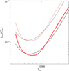 |
Fig. A.3. Conversion factor between observed CoRoT flux and bolometric flux as a function of spectral parameters/shape and extinction. The |


where ACoRoT can be derived from AV and Eq. (A.1). Figure A.3 shows the ratio in Eq. (A.5) as a function of spectral parameters, Teff and log g for stellar spectra, or temperature for black body spectra, and of interstellar extinction, AV. All solid lines refer to the case of AV = 0.0. The four thin red lines refer to the stellar case with the four values of log g that we have explored. The thicker red line shows the mean of the four values at each Teff, and is the curve we have adopted throughout this paper when converting observed flare fluxes to bolometric fluxes, when adopting stellar-like spectra. The thick black line refers to black body emission spectra. Finally, the dotted red and black lines show the  ratio for the stellar and black-body cases, respectively, for an AV = 1.0 mag interstellar extinction.
Appendix B: Lightcurves of X-ray flares with CoRoT and/or Spitzer counterparts
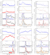 |
Fig. B.1. Lightcurves of all X-ray flares with counterparts in the optical and/or mIR bands. See caption of Fig. 2 for a full description of the content of each panel. |
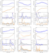 |
Fig. B.1. continued. |
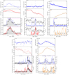 |
Fig. B.1. continued. |
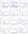 |
Fig. B.1. continued. |
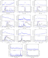 |
Fig. B.1. continued. |
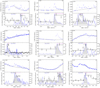 |
Fig. B.1. continued. |
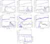 |
Fig. B.1. continued. |
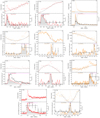 |
Fig. B.1. continued. |
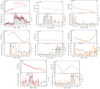 |
Fig. B.1. continued. |
Appendix C: X-ray flares with a possible CoRoT/Spitzer counterpart
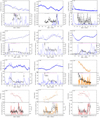 |
Fig. C.1. Lightcurves of all X-ray flares with a possible but not well-defined counterpart in the optical and/or mIR bands. See caption of Fig. 2 for a full description of the content of each panel. |
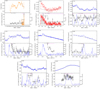 |
Fig. C.1. continued. |
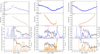 |
Fig. C.1. continued. |
Appendix D: X-ray flares within the Chandra observing segments and with no CoRoT or Spitzer counterpart
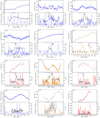 |
Fig. D.1. Lightcurves of all detected X-ray flares fully included in the Chandra observing segments and for which no obvious counterpart is observed in the optical and/or mIR bands. See caption of Fig. 2 for a full description of the content of each panel. |
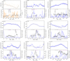 |
Fig. D.1. continued. |
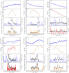 |
Fig. D.1. continued. |
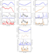 |
Fig. D.1. continued. |
All Tables
All Figures
|
Fig. 1. Left: spatial distribution of likely NGC 2264 members with simultaneous lightcurves, highlighting those undergoing simultaneous X-ray+optical and/or X-ray+mIR flaring. X-symbols: all Chandra sources in the “simultaneous” FOVs. Circles: Chandra+CoRoT sources (with unique identifications). Squares: Chandra+Spitzer sources. Green and orange symbols indicate sources with simultaneous X-ray+optical and X-ray+mIR flaring, respectively. Blue crosses indicate stars with a well observed X-ray flare having no counterpart in other available bands (Sect. 6.3 and Appendix D). Note the smaller spatial coverage, but better completeness with respect to the X-ray sources, of the mIR sample with respect to the optical one. Right: same as above in the log LX vs. J-magnitude plane, showing the deeper coverage of mIR data and the tendency of flares to be detected on the stars with higher average X-ray luminosity. |
| In the text | |
|
Fig. 2. Lightcurves of six of the X-ray flares with optical and/or mIR counterpart discussed in the text. Lightcurves for the full sample can be found in Appendix B, while lightcurves for well defined X-ray flares for which no optical/mIR counterpart was detected are shown in Appendix C. The three panels at the top refer to flares with simultaneous data in all three bands. Within each panel the first two sub-panels, from top to bottom, show the CoRoT lightcurve, normalized to the median of the observed CoRoT flux in the whole exposure (as opposed to the short segment shown), and the Spitzer lightcurve in the IRAC 3.6 μm or 4.5 μm bands (as indicated by the y-axis label and in orange and red, respectively). For both panels a gray line indicate the polynomial intended to represent the non-flaring emission (see text). The ACIS source number of the star and its mIR class are given at the top-left and top-right corners, respectively. The third and fourth panels show the same CoRoT and Spitzer lightcurves, this time subtracted by the non-flaring emission (units given in the right-hand y-axis). The areas shaded in gray indicate our choice for the definition of the optical and mIR flares. The same two panels show the simultaneous Chandra X-ray lightcurve, both binned (black dots with error bars), and using the piece-wise representation discussed in the text (black broken line). Units are shown on the left-hand y-axis. The temporal extension of the X-ray flare, according to our definition, is indicated by a magenta horizontal bar at the top of each panel. The three panels at the bottom show three more X-ray flares with simultaneous CoRoT data, but lacking Spitzer data. |
| In the text | |
|
Fig. 3. Left: total “bolometric” emitted energy, Eopt, estimated from the CoRoT lightcurves (see text) vs. energy emitted in the 0.5–8.0 keV band, EX. Green and red circles indicate flares from Class III and Class II stars, respectively. Filled circles refer to the flares in our main samples, empty ones to flares with particularly uncertain estimates. The dashed lines shows the unit relation, while the solid lines show the results of six different linear fits (in the log–log plane) performed with different methods, and whose parameters are shown in the upper part of the panel along with the 1σ dispersion of residuals. The fitting methods are: (1) Ordinary Least Squares Y vs. X, (2) Ordinary Least Squares X vs. Y, (3) Ordinary Least Squares Bisector, (4) Orthogonal Reduced Major Axis, (5) Reduced Major-Axis, (6) Mean ordinary Least Squares. Right: same as the plot on the left, but for peak luminosities instead of energies. |
| In the text | |
|
Fig. 4. Left: bolometric flare emitted energy, estimated from the Spitzer lightcurves assuming a 104 K black body spectrum, EIR, vs. EX the energy emitted in the 0.5–8.0 keV band. Symbols and lines as in Fig. 3/5, with the addition of blue circles, which indicate flares from Class I sources. Right: same as the plot on the left, but for peak luminosities instead of energies. |
| In the text | |
|
Fig. 5. EIR/Eopt vs. EX (left) and LIR, pk/Lopt, pk vs. LX, pk (right). Eopt and Lopt are derived either from the analysis of the CoRoT lightcurves (shown as circles) or estimated from the X-ray quantities and the correlation with the optical ones (squares). The remaining symbols are as in Fig. 4. The vertical scale on the right-hand axes indicate the temperature of the black body spectrum, assumed to be responsible for the emission in the optical and IR bands. The results of KS tests comparing the distributions of the optical/IR ratios for flares from Class II and Class III sources are shown in the upper-left corner, both for the higher quality flares (filled symbols) and for all flares. Note that, at least for the higher quality flares, the null probabilities reported indicate that the distributions are significantly different. |
| In the text | |
|
Fig. 6. Comparisons between the duration of flares in different bands. The three panels show all three possible comparison between the X-ray, optical, and mIR bands. Duration are defined as described in the text, as the ratio between integrated energy and peak luminosity. Flares plotted as squares are those observed in all three bands. The remaining symbols and colors are as in Figs. 3 and 4. The thick gray diagonal line indicates the unit relation. Thinner lines deviations by factors of 0.5, 2.0, 4.0, and 8.0. The results of KS tests comparing the distributions of the ratios of the two plotted quantities for flares from Class II and Class III sources are shown in the upper-left corner, both for the higher quality flares (filled symbols) and for all flares. The null probabilities reported do not evidence any significant difference. |
| In the text | |
|
Fig. 7. Distributions of time delays between the flare start times in the optical band vs. X-rays (left panel), IR vs. X-rays (center), and optical vs. IR bands (right). Distributions for flares on Class II and Class III stars are plotted separately in each panel in red and green, respectively. The results of KS tests comparing the two distributions are shown in the lower-left corner, indicating in all cases that the distributions are not significantly different. |
| In the text | |
|
Fig. 8. Solid black lines: cumulative distributions of residuals in the linear fits to the log Lopt, pk vs. log LX, pk scatter plot. Each line refers to one of the six linear fits shown in Fig. 3. Dashed orange line: predicted distributions assuming the optical peak luminosity is perfectly correlated to the X-ray peak luminosity and that the observed optical flux, from an optically thick slab-like region, is attenuated by projection effects (see text). Dashed green line: same as above with an additional attenuation due to limb darkening. The fact that the observed scatter is smaller than predicted by these assumption, even ignoring measurement uncertainties and flare-to-flare variations, indicates that the assumptions on the optical emitting regions are not correct. |
| In the text | |
|
Fig. A.1. Extinction laws for the CoRoT band (in black) and for the V, Rc, and Ic optical filters (green, red, and orange, respectively). The thin lines show the variation of A(band)/AV with effective temperature for the stellar-like spectra with log g between 3.0 and 4.5. Thicker lines show the trend of A(band)/AV with temperature for black body spectra. |
| In the text | |
|
Fig. A.2. Ratio between observed CoRoT flux, in instrumental units, and the flux predicted from model spectra vs. observed R magnitudes. The plotted points refer to a subsample of suitable and well characterized NGC 2264 members (see text), and symbols of different colors, largely overlapping with each other, refer to estimates obtained assuming four different values of log g between 3.0 and 4.5. The horizontal line refers to the adopted value, 4.2 × 10¹⁵ erg−1 s−1 cm−2. |
| In the text | |
|
Fig. A.3. Conversion factor between observed CoRoT flux and bolometric flux as a function of spectral parameters/shape and extinction. The |
| In the text | |
|
Fig. B.1. Lightcurves of all X-ray flares with counterparts in the optical and/or mIR bands. See caption of Fig. 2 for a full description of the content of each panel. |
| In the text | |
|
Fig. B.1. continued. |
| In the text | |
|
Fig. B.1. continued. |
| In the text | |
|
Fig. B.1. continued. |
| In the text | |
|
Fig. B.1. continued. |
| In the text | |
|
Fig. B.1. continued. |
| In the text | |
|
Fig. B.1. continued. |
| In the text | |
|
Fig. B.1. continued. |
| In the text | |
|
Fig. B.1. continued. |
| In the text | |
|
Fig. C.1. Lightcurves of all X-ray flares with a possible but not well-defined counterpart in the optical and/or mIR bands. See caption of Fig. 2 for a full description of the content of each panel. |
| In the text | |
|
Fig. C.1. continued. |
| In the text | |
|
Fig. C.1. continued. |
| In the text | |
|
Fig. D.1. Lightcurves of all detected X-ray flares fully included in the Chandra observing segments and for which no obvious counterpart is observed in the optical and/or mIR bands. See caption of Fig. 2 for a full description of the content of each panel. |
| In the text | |
|
Fig. D.1. continued. |
| In the text | |
|
Fig. D.1. continued. |
| In the text | |
|
Fig. D.1. continued. |
| In the text | |
Current usage metrics show cumulative count of Article Views (full-text article views including HTML views, PDF and ePub downloads, according to the available data) and Abstracts Views on Vision4Press platform.
Data correspond to usage on the plateform after 2015. The current usage metrics is available 48-96 hours after online publication and is updated daily on week days.
Initial download of the metrics may take a while.