| Issue |
A&A
Volume 620, December 2018
|
|
|---|---|---|
| Article Number | A111 | |
| Number of page(s) | 18 | |
| Section | Extragalactic astronomy | |
| DOI | https://doi.org/10.1051/0004-6361/201832729 | |
| Published online | 05 December 2018 | |
Kinematics of the outer halo of M 87 as mapped by planetary nebulae⋆,⋆⋆
1
Kavli Institute for Astronomy and Astrophysics, Peking University, 5 Yiheyuan Road, 100871
Beijing, PR China
e-mail: This email address is being protected from spambots. You need JavaScript enabled to view it.
2
Max-Planck-Institut für Extraterrestrische Physik, Giessenbachstrasse, 85741
Garching, Germany
e-mail: This email address is being protected from spambots. You need JavaScript enabled to view it.
, This email address is being protected from spambots. You need JavaScript enabled to view it.
3
European Southern Observatory, Karl-Schwarzschild-Strasse 2, 85748
Garching, Germany
Received:
29
January
2018
Accepted:
23
September
2018
Abstract
Aims. We present a kinematic study of a sample of 298 planetary nebulas (PNs) in the outer halo of the central Virgo galaxy M 87 (NGC 4486). The line-of-sight velocities of these PNs are used to identify subcomponents, to measure the angular momentum content of the main M 87 halo, and to constrain the orbital distribution of the stars at these large radii.
Methods. We use Gaussian mixture modelling to statistically separate distinct velocity components and identify the M 87 smooth halo component, its unrelaxed substructures, and the intra-cluster (IC) PNs. We compute probability weighted velocity and velocity dispersion maps for the smooth halo, and its specific angular momentum profile (λR) and velocity dispersion profile.
Results. The classification of the PNs into smooth halo and ICPNs is supported by their different PN luminosity functions. Based on a Kolmogorov–Smirnov (K–S) test, we conclude that the ICPN line-of-sight velocity distribution (LOSVD) is consistent with the LOSVD of the galaxies in Virgo subcluster A. The surface density profile of the ICPNS at 100 kpc radii has a shallow logarithmic slope, −αICL ≃ −0.8, dominating the light at the largest radii. Previous B − V colour and resolved star metallicity data indicate masses for the ICPN progenitor galaxies of a few ×108 M⊙. The angular momentum-related λR profile for the smooth halo remains below 0.1, in the slow rotator regime, out to 135 kpc average ellipse radius (170 kpc major axis distance). Combining the PN velocity dispersion measurements for the M 87 halo with literature data in the central 15 kpc, we obtain a complete velocity dispersion profile out to Ravg = 135 kpc. The σhalo profile decreases from the central 400 km s−1 to about 270 km s−1 at 2–10 kpc, then rises again to ≃300 ± 50 km s−1 at 50–70 kpc, to finally decrease sharply to σhalo ∼ 100 km s−1 at Ravg = 135 kpc. The steeply decreasing outer σhalo profile and the surface density profile of the smooth halo can be reconciled with the circular velocity curve inferred from assuming hydrostatic equilibrium for the hot X-ray gas. Because this rises to νc,X ∼ km s−1 at 200 kpc, the orbit distribution of the smooth M 87 halo is required to change strongly from approximately isotropic within Ravg ∼ 60 kpc to very radially anisotropic at the largest distances probed.
Conclusions. The extended LOSVD of the PNs in the M 87 halo allows the identification of several subcomponents: the ICPNs, the “crown” accretion event, and the smooth M 87 halo. In galaxies like M 87, the presence of these subcomponents needs to be taken into account to avoid systematic biases in estimating the total enclosed mass. The dynamical structure inferred from the velocity dispersion profile indicates that the smooth halo of M 87 steepens beyond Ravg = 60 kpc and becomes strongly radially anisotropic, and that the velocity dispersion profile is consistent with the X-ray circular velocity curve at these radii without non-thermal pressure effects.
Key words: galaxies: clusters: individual: Virgo cluster / galaxies: halos / galaxies: individual: M 87 / stars: abundances / planetary nebulae: general
Based on observations made with the VLT at Paranal Observatory under programmes 088.B-0288(A) and 093.B-066(A), and with the Subaru Telescope under programme S10A-039.
Table B.1 is only available at the CDS via anonymous ftp to cdsarc.u-strasbg.fr (130.79.128.5) or via http://cdsarc.u-strasbg.fr/viz-bin/qcat?J/A+A/620/A111
© ESO 2018
1. Introduction
Several studies are currently concentrating on the dramatic size growth of passive galaxies with redshift (van Dokkum et al. 2010; Cimatti et al. 2012) with the goal of establishing the structural analogues in local massive galaxies. Within the cosmological framework, a variety of different models have been put forward to explain the mass/size growth (see e.g. Huang et al. 2013), among which the two-phase formation scenario appears to be in the best agreement with observational constraints. In this scenario, the innermost region of massive galaxies formed the majority of their stars at z ≤ 3 on short timescales (Thomas et al. 2005), while the stars in the outermost regions were accreted at later epochs as a consequence of mostly dry mergers or accretion events (Oser et al. 2010, 2012; Cook et al. 2016). Then the outermost regions of local massive galaxies should contain the fossil records of the accretions events in form of spatial and kinematic substructures because the growth is expected to occur at comparatively low redshifts and the dynamical timescales are long (Bullock & Johnston 2005).
In the local universe, massive galaxies are found in the densest regions of galaxy clusters, hence a fraction of the stars in their extreme outer regions might in fact be part of the intra-cluster light (ICL), i.e. a stellar component that is not gravitationally bound to a single galaxy, but orbits in the cluster potential. A galaxy’s halo and the ICL both result from hierarchical accretion; however, they differ in their kinematics and their different levels of dynamical relaxation (Dolag et al. 2010; Longobardi et al. 2015a; Cooper et al. 2015; Barbosa et al. 2018). Analysis of the radius versus line-of-sight velocity (LOSV) projected phase-space for several massive nearby galaxies, e.g. NGC 1399 (Schuberth et al. 2010; McNeil et al. 2010) and M 87 (Longobardi et al. 2015a), found that halo and ICL need to be treated separately in order to avoid systematic biases in the mass estimates at large radii.
In massive early-type galaxies, surface brightness profiles are a possible avenue to disentangle multiple components, those generated by early dissipative processes or late epoch accretions, or the ICL. The presence of an accreted component is usually inferred from the change in slope of the galaxy’s light profile at large radii (Zibetti et al. 2005; Gonzalez et al. 2007; D’Souza et al. 2014; Spavone et al. 2017), from high Sersic indices (Kormendy et al. 2009, n > 4) and/or from variations in the ellipticity profile (Tal & van Dokkum 2011; D’Souza et al. 2014; Mihos et al. 2017). One open question is whether the decomposition of the surface brightness profile in multiple components is supported independently by the stellar kinematics (Hernquist & Barnes 1991; Hoffman et al. 2010; Emsellem et al. 2004, 2014). In the interesting case of NGC 6166, the best Sersic fit decomposition of the surface brightness profile fails to reproduce the transition between the low-velocity dispersion of the central region and the kinematically hotter envelope at radii larger than 10 kpc (Bender et al. 2015).
Therefore, a kinematic decomposition is required to unambiguously resolve the physical components. At large radii where the galaxy surface brightness is too low for standard absorption line spectroscopy, this can only be done with discrete tracers such as globular clusters (GCs) and planetary nebulas (PNs). If we were able to measure surface brightness profiles and kinematics at large radii, we would (1) find the predicted accretion structures where they have not phase mixed yet; (2) isolate the kinematics of the phase-mixed, smooth halo to constrain its orbit distribution and obtain unbiased estimates of enclosed mass; and (3) understand the transition between halo and ICL.
Recent surveys of bright, discrete probes such as GCs and PNs have enabled the systematic studies of the physical properties of early-type galaxy halos. GCs are compact, bright sources easily identified on high-resolution images (Côté et al. 2001; Schuberth et al. 2010; Strader et al. 2011; Romanowsky et al. 2012; Pota et al. 2013). PNs, because of the strong [OIII]λ5007Å emission line from their envelope re-emitting up to ∼15% of the UV luminosity of the central star (Dopita et al. 1992), have been the targets of several surveys that aim to trace light and motions of single stars in nearby galaxies and clusters (Hui et al. 1993; Méndez et al. 2001; Peng et al. 2004; Coccato et al. 2009; McNeil et al. 2010; McNeil-Moylan et al. 2012; Cortesi et al. 2013; Longobardi et al. 2013, 2015a,b; Hartke et al. 2017; Pulsoni et al. 2018), and out to distances of 50–100 Mpc (Gerhard et al. 2005; Ventimiglia et al. 2011).
The Virgo cluster, which is the nearest large-scale structure, and its central galaxy M 87 are prime targets for addressing the subject of galaxy evolution in clusters. The Virgo cluster shows a number of spatial and kinematic substructures, with different subgroups having different mixtures of morphological galaxy types (Binggeli et al. 1987). The evidence that many galaxies are presently in-falling towards the cluster core, and the presence of a complex network of extended tidal features revealed by deep photometric surveys suggest that the Virgo cluster core is not yet in dynamical equilibrium.
The giant elliptical galaxy M 87 is close to the dynamical centre of the Virgo cluster (Binggeli et al. 1987; Nulsen & Bohringer 1995; Mei et al. 2007). It is classified as a cD-galaxy, nicely described by a single Sersic fit with n ∼ 11 (Kormendy et al. 2009; Janowiecki et al. 2010) and an extended halo that reaches out to R ∼ 150−200 kpc. Its total stellar mass is estimated to be M ∼ 1012 M⊙. The dynamical structure of M 87 is dominated by random motions, without significant rotation (van der Marel 1994; Sembach & Tonry 1996; Gebhardt et al. 2011). A low-amplitude kinematically distinct core (Emsellem et al. 2014), a slow rotational component (Murphy et al. 2011; Emsellem et al. 2014), and a rising stellar velocity dispersion profile with radius (Murphy et al. 2011) were measured in recent studies. Several independent tracers were used to probe the mass distribution of M 87: X-ray measurements (Nulsen & Bohringer 1995; Churazov et al. 2010), integrated stellar kinematics (Murphy et al. 2011, 2014), GC kinematics (Côté et al. 2001; Strader et al. 2011; Romanowsky et al. 2012; Zhu et al. 2014), and PN kinematics (Arnaboldi et al. 2004; Doherty et al. 2009). All of these studies show consistently that M 87 is one of the most massive galaxies in the local Universe, but there are considerable variations among studies using different tracers.
Of particular interest is whether the hot (T ∼ 1 keV) low-density (n < 0.1 cm−3) X-ray envelope (Forman et al. 1985) around M 87 is quiescent enough to assume hydrostatic equilibrium. In this case, we can use the temperature and density profiles derived from the X-ray spectra to obtain the cumulative mass profile and gravitational potential, and then estimate the orbital anisotropy of the stars from their dispersion profile. Non-thermal contributions to the pressure measured from X-ray data can be studied by comparing the potential inferred from the X-rays with mass estimates from stellar kinematics (e.g. Churazov et al. 2008, 2010).
The goal of this paper is to identify the PNs in the smooth M 87 halo, using accurate velocities and following the approach of Longobardi et al. (2015a). We work with the sample of 253 PNs M 87 halo PNs1 and the 45 intra-cluster (IC) PNs, for which LOSVs are available with an estimated median velocity accuracy of 4.2 km s−1. We determine the rotation ν and velocity dispersion σ for the M 87 halo in the region from ∼20 kpc to ∼200 kpc. From these measured profiles we aim to answer the question whether the halo stellar population, its mean square velocity, and its degree of relaxation change smoothly with radius, such that it eventually reaches ICL properties, or whether the halo and ICL are distinct populations and dynamical components. Furthermore, we investigate whether the halo dispersion profile is consistent with the mass profile inferred from X-rays and what this tells us about the orbital anisotropy and its variations in the outer halo region.
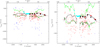 |
Fig. 1. Left: projected phase-space diagram VLOS vs. major axis distance R from the centre of M 87 out to 200 kpc for all spectroscopically confirmed PNs from Longobardi et al. (2015a); their M 87 halo PNs (red asterisks) and ICPNs (blue asterisks) are shown separately; R > 0 and R < 0 represent the northern and southern halves with respect the galaxy centre. Red open circles show four newly identified kinematic outliers (see Sect. 2.2). Black dash-dotted and black continuous lines depict the running average and running velocity dispersion independently for the M 87 south-east and north-west, computed from the 253 halo PNs. Full red circles show the robust estimate of the halo velocity dispersion following Longobardi et al. (2015a), while full black circles show the velocity dispersion values after probability-weighted removal of the crown substructure from Longobardi et al. (2015b). Both velocity dispersion profiles (red and black circles) show strong radial variation, with a steep decline at major axis distances R > 100 kpc. Green dash-dotted and green continuous lines show the running average and velocity dispersion for the combined sample of 253 halo PNs and 45 ICPNs; the inclusion of ICPNs leads to a rapidly rising velocity dispersion profile. Cyan triangles show the velocity dispersion measurements from the IFU VIRUS-P data of Murphy et al. (2011, 2014) whose outer rise near R = 700″ (∼40 kpc) is matched by the running joint halo and ICPN velocity dispersion (green line) indicative of the contribution from the ICL. Right: zoomed-in plot in the velocity range ±1000 km s−1 centred on the systemic velocity of M 87. |
The paper is structured as follows. In Sect. 2 we revisit the PN LOSV distribution (LOSVD) and re-identify M 87 halo PNs and ICPNs. In Sect. 3 we estimate the smoothed velocity field for the M 87 halo PNs, and determine the amplitude of rotation and the λ(R) angular momentum parameter as a function of radius. In Sect. 4 we determine our fiducial composite velocity dispersion profile for M 87 and derive the circular velocity curve from a simple Jeans model. This circular velocity curve is then compared with that measured from X-ray observations in Churazov et al. (2010). Finally, we discuss our results in Sect. 5 and give our conclusions in Sect. 6). In the Appendix, we provide the detailed PN LOSVDs for the outer halo of M 87 in different radial bins and the complete M 87 PN catalogue using the data from the PN photometric and spectroscopic surveys carried out with Suprime-Cam mounted on the Subaru Telescope and the FLAMES spectrograph installed on the VLT.
In this work the systemic velocity of M 87 is Vsys = 1307.0 ± 7 km s−1 (Allison et al. 2014), and we adopt a distance modulus of 30.8 for M 87 (Longobardi et al. 2015a), implying a physical scale of 73 pc arcsec−1.
2. Kinematics of M 87 and the Virgo intra-cluster stars
We begin our investigation on the kinematics of halo and IC PNs by adopting a similar approach to that of Longobardi et al. (2015a) who applied a robust sigma estimator (McNeil et al. 2010) to separate the asymmetric broad wings of the LOSVD of the ICL, from the nearly symmetric main distribution of velocities centred at the systemic velocity of M 87, the galaxy halo.
The halo-ICL dichotomy is illustrated in Fig. 1 where we show the projected phase-space distribution for halo (red asterisks) and IC (blue asterisks) PNs, VLOS versus major axis distance, on the basis of the classification by Longobardi et al. (2015a). Because the two components overlap in velocity, Longobardi et al. (2015a) argued that a fraction of the PNs whose LOSV values are in the range of the M 87 main halo may also be IC PNs; this is investigated further in Sect. 2.3.
To illustrate the effect of the ICL on the velocity dispersion profile, we compute the LOSVD running average and running dispersion2 for the total PN sample (M 87 halo plus ICPNs, green lines) and for the halo PNs only (black lines), independently on both sides of the M 87 major axis. While the mean velocity curves are very similar, the running dispersion curves are widely different. The running dispersion of the M 87 plus IC PNs (green line) quickly rises to a value which is similar to the velocity dispersion of the Virgo subcluster A/Virgo core ∼700 km s−1 (Binggeli et al. 1987; Conselice et al. 2001) with no further radial variation on both sides of the M 87 major axis. The running dispersion of only the M 87 halo PNs behaves differently: it is almost constant at 270−290 km s−1 out to 30–40 kpc and then shows a rise at about 70 kpc, followed by a steep decline.
We emphasise that the strong radial variations in the running dispersion for the M 87 halo PN LOSV are measured independently on both sides of the galaxy. Furthermore, the drop to small values of the running dispersion at the largest major axis distances is significant because (1) it is observed over several subsequences of the halo running dispersion, (2) the running dispersion curve reaches small values on both sides of the M 87 photometric major axis, and (3) the measurements of the M 87 halo PN velocities come from two independent data sets. In the north of M 87, i.e. for R > 0 in Fig. 1, the outermost PN velocities were measured by Doherty et al. (2009), while in the south of M 87, i.e. R < 0 in Fig. 1, the measured velocities are from Longobardi et al. (2015a). The typical velocity errors are 4.2 km s−1 for the PNs from Longobardi et al. (2015a), and ∼3.0 km s−1 for PNs from Doherty et al. (2009).
Binning the PN velocities in Fig. 1 in six elliptical bins with major axis distances in the range 20 kpc < R < 170 kpc, we compute the velocity dispersion profile for the M 87 halo plus IC PNs. We also compute the halo-only velocity dispersions in these bins, using the robust estimator from McNeil et al. (2010) as described in Longobardi et al. (2015a). These values are given in Table 1, and the halo dispersions are plotted in Fig. 1 (full black circles).
For the M 87 halo plus IC PN LOSV sample, the velocity dispersion increases from σhalo+ICL ≃ 243.6±69.5 km s−1 at R ≃ 20 kpc to σhalo+ICL = 794.6±67.8 km s−1, at R = 120 kpc. For the M 87 halo PNs only, the velocity dispersion is almost constant at a value of σrobust halo = 268.9±48.4 km s−1 between 20 and 70 kpc. It then increases to σrobust halo = 361.7 ± 26.5 km s−1, at R = 90 kpc, and then declines steeply at larger radii, reaching σrobust halo = 154.6 ± 36.4 km s−1 at R = 170 kpc.
In Fig. 1, we also plot the M 87 velocity dispersion measurements from the integrated stellar light using the IFU VIRUS-P (Murphy et al. 2011, 2014). These measurements indicate a steep increase in the two outermost bins at R > 30 kpc. The comparison with the PN velocity dispersion suggests that the reason for the rise in the velocity dispersion in the IFU kinematics is the contribution of the ICL at large distances where we expect the M 87 stellar halo surface brightness to decrease rapidly and the ICL to become significant.
Velocity dispersion estimates from the PN sample in the outer region of M 87.
Having realised the contribution of the Virgo IC stars to the kinematics of the outer regions of M 87, we now focus on the galaxy halo. In the following sections we investigate whether the strong radial dependence observed in the σrobust halo is an intrinsic property of the M 87 halo or whether it signals the presence of additional velocity components.
2.1. A shell in a sea of stars: the kinematic footprint of the crown of M 87
Direct evidence of a low-mass satellite accretion onto the M 87 halo comes from the cold features observed in the projected phase-space of discrete PNs and GCs (Longobardi et al. 2015b; Romanowsky et al. 2012) and from the orbital properties of GCs (e.g. Agnello et al. 2014) and ultra-compact dwarfs (UCDs; Zhang et al. 2015). Once these cold substructures are identified in phase space, we can recover the kinematics of the main halo component.
In their recent study, Longobardi et al. (2015b) used Gaussian mixture models (GMMs) to statistically separate the PNs of their newly discovered “crown” substructure from the LOSVD of the 253 M 87 halo PNs as classified by Longobardi et al. (2015a). This resulted in a total of 53 PNs that had a small average probability (γi ∼ 0.3) of being part of the M 87 main halo. We now use this information and compute the velocity dispersion of the remaining M 87 halo. As seen in Fig. 1 (red and black full dots, respectively), the sigma profile without the crown does not change substantially. The contribution by the accreted satellite reduces the LOS velocity dispersion in those radial bins where the number of crown stars is largest. It is clear that the strong radial variation in the velocity dispersion profile remains an intrinsic property of the M 87 main halo.
2.2. Outliers in the M 87 halo
In Fig. 1, we see two pairs of PNs in the southern region of M 87 (at negative distances), where the two PNs in each pair have very similar positions and velocities (red circles). Both PN pairs are clearly outside the velocity distribution of their neighbours. We now determine how likely such velocity configurations are by using conditional probability theory, which states that the probability of event Vi and event Vj is
 (1)
(1)
i.e. the probability of event Vi times the probability of event Vj given that event Vi occurred. In our case we can assume that the first PN of each pair is at a random position and velocity just like most other PNs, so the relevant probability is P(Vj|Vi).
P(Vj|Vi) has two parts, a photometric part Pphot that is the probability of finding a second PN within the measured relative distance dD to the first, and a kinematic part Pkin that is the probability of finding it within the measured dV = ∥Vi − Vj∥ from the first PN. The photometric part can be estimated from the PN number density at the position of the PNe, which gives the expected probability of finding one PN within π(dD)2. The kinematic probability is given by the integral of the normalised LOSVD over the range Vi ± dV. Using the halo PN number density profile from Sect. 2.3.3 below and a Gaussian halo velocity distribution centred on Vsys = 1307 km s−1 and with dispersion σ ∼ 300 km s−1, the probability P(Vj|Vi) = Pphot × Pkin of observing both pairs of PNs is < 0.3%.
These low values support the classification of these PNs as kinematic outliers, even if their velocities overlap with the range of velocities for the M 87 main halo. It is interesting to note that these PN pairs close to M 87 overlap spatially with a photometric stream in the southern part of M 87, recently identified by Mihos et al. (2017). These authors interpreted this photometric feature as debris from a tidally dissolved dwarf galaxy (marked as small arrow in the central panel of their Fig. 5). Thus, from here on the four PNs are flagged as outliers and assigned to the ICL.
2.3. Residual contributions from the ICL to the M 87 halo LOSVD
We now analyse in more detail the LOSVD of the remaining M 87 halo and investigate whether it contains residual contributions from the ICL. In what follows we examine the generalised histogram where each PN is represented by a Gaussian distribution3, weighted by its membership probability, γi, of belonging to the M 87 halo.
In Fig. 2 we show the generalised histogram for four M 87 halo PN (sub)samples. These are (i) the M 87 halo PNs from Longobardi et al. (2015a), (ii) the PNs along the minor axis only and the PNs along the major axis, and (iii) north of and (iv) south of the M 87 centre (see the insets in each panel with the selected PNs depicted in red). All LOSVDs for the four subsamples show a multi-peaked distribution, with a second peak observed in all four histograms, centred at νII ≃ 1000 km s−1.
In order to verify whether this second peak is statistically significant we performed a Monte Carlo analysis. We simulated 100 LOSVDs that were drawn from a single Gaussian distribution with sample size matching the number of the M 87 halo PN sample. For each of the 100 simulated LOSVD, we randomly extracted three subsamples to simulate the LOSVD along the minor axis, and the major axis north and south. Only 18% of the simulated sets of LOSVDs show a double-peaked structure in all four subsamples. Hence, we are confident at the 82% level (1.5 × σ) that the feature corresponding to the second peak is real.
In Fig. 2 the distributions along the minor axis and major axis north show an additional third peak at νIII ≃ 1800 km s−1. However, we note that this feature is more likely to occur as the result of low number statistics, with a probability higher than 50%, i.e. less than 1.0 × σ.
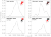 |
Fig. 2. Generalised histogram for (i) the entire M 87 halo PN LOSVD (top left), (ii) the subsample along the minor axis (top right), and (iii) the subsample along the major axis north (bottom left) and (iv) south (bottom right) of M 87. The PNs for each subsample are depicted in red in the spatial distributions shown in the top right corner of each panel. All histograms show a multi-peaked distribution, with a secondary peak at ∼1000 km s−1. The probability that such a secondary peak is caused by low number statistics is ∼18% (see text for details). |
2.3.1. Gaussian mixture model for the M 87 halo LOSVD: identification of the νII ≃ 900 km s−1 peak
Following Longobardi et al. (2015b), we assume that the remaining M 87 halo LOSVD can be described by a mixture of K Gaussian distributions, and use a GMM to identify the individual kinematic structures (see Pedregosa et al. 2011; Longobardi et al. 2015b for more details). The GMM implements the expectation-maximisation (EM) algorithm for fitting mixture-of-Gaussian models. However, our estimated Gaussian mixture distribution starts from a weighted sample as we already removed the crown contribution statistically. We modified the GMM routine accordingly.
In this case we have a set of weighted data, xi, the PN velocities in our case, where each measurement has a corresponding weight, γi. We want to estimate the parameters of a Gaussian mixture distribution using this set of weighted data. The Gaussian density function (PDF) can be written as
where pk(x | μk, σk)Pk is the individual mixture component centred on μk with a dispersion σk, and Pk is the mixture weight. The EM procedure is as follows:
-
E-step: Computing the posterior probabilities of the ith measurement to belong to the kth Gaussian components at step m, weighted by γi,
where
 .
. -
M-step: Computing the new parameter estimates
Hence, the- step in the EM process has been modified such that the posterior probability of the ith measurement of belonging to the kth Gaussian at step m,  , always carries the starting weight γi of that measurement. At the end of the algorithm, each PN velocity is allocated a posterior probability that quantifies its association with each Gaussian component, denoted Γi, k. Subsequently, we use Γi = Γi, 1 to denote the probability of belonging to the smooth halo component.
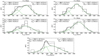 |
Fig. 3. Histograms of the LOSVD along the M 87 major (top four panels) and minor axis (bottom centre panel). The larger number of tracers associated with the M 87 halo allows us to divide the halo PN sample into northern (top left panels) and southern (top right panels) subsamples; moreover, the PN subsamples along the major axis are further divided in two elliptical bins, as given in the panels. The best-fit GM model (thick black line) identifies in all subsamples two Gaussian components (green lines). Dashed histograms represent the PN LOSVD prior to the statistical subtraction of the crown substructure. |
We run the GMM on the M 87 halo PN subsamples along the minor axis, and the major axis north and south (Fig. 2 top right and bottom panels). Moreover, as we have higher number statistics, the major axis samples are further divided into two elliptical bins covering radial ranges R ≤ 55 kpc and R > 55 kpc. The GMM identifies the double-peak structure in all these subsamples, for which we show the histograms of the data along with the best-fit GMM in Fig. 3.
The M 87 halo PN LOSVD is then decomposed into two Gaussian mixtures. The main component contributes about 80% of the total PN sample and is centred at the systemic velocity of M 87, νsys = 1307 km s−1 (see Table 3). Within the uncertainties, there is no significant variation in its central velocity along the northern side of the galaxy; however, south of M 87 and for R > 5 kpc, it peaks at 1378.2 ± 39.5 km s−1, suggesting the presence of ordered motion along the LOS at these distances (see Sect. 3 for a more detailed analysis). The velocity dispersion values averaged over the southern and northern major axis increase from σhalo = 242.1 ± 22.3 km s−1 at R ≤ 55 kpc to σhalo = 299.7 ± 26.2 km s−1 for R ≤ 55 kpc. Along the minor axis, the velocity dispersion of the main component is larger, with σhalo = 367.6 ± 44.0 km s−1, but still within 1.5σ of the values measured in the outermost bin along the major axis.
The second Gaussian component is centred at νII = 888.7 ± 23.1 km s−1, with a nearly constant velocity dispersion, σII ± 97.9 km s−1. In the following, we call this the νII ≃ 900 km s−1 component. Its mean velocity is constant along the major axis within the uncertainties. However, along the minor axis it has a higher value: νII, minor axis = 1050.7 ± 30.7 km s−1. The contribution of the secondary component to the total LOSVD does not vary across the galaxy and contributes a total of 24 PNs, representing ∼10% of the PN sample associated with the M 87 halo in Longobardi et al. (2015a). For completeness, all the Gaussian fitting parameters are listed in Table 2.
2.3.2. The ICPN LOSVD: comparison with the velocity distribution of the galaxies in the Virgo cluster core
We now ask the question about the origin of the second Gaussian component in the M 87 halo LOSVD. Dynamical studies of the bright central regions of non-rotating elliptical galaxies show that their LOSVDs are nearly Gaussian, with deviations of the order of 2% (Gerhard 1993; Bender et al. 1994). The secondary component in the M 87 halo LOSVD contributes 10% of the total; it clearly represents a larger deviation from a single-Gaussian velocity distribution. We note that its average velocity, νII = 888.7 ± 23.1 km s−1, is close to the mean value determined for the velocity distribution of galaxies in the Virgo subcluster A (Binggeli et al. 1987). This suggests that this kinematic component could be a part of the Virgo ICL.
Gaussian fitting parameters from the GMM decomposition of the M 87 halo PN LOSVD for the subsamples along the minor axis, major axis north, and major axis south.
We can sharpen the argument further by comparing the LOSVD of all identified ICPNs, including the νII ≃ 900 km s−1 component, to the LOSVD of the galaxies in the Virgo subcluster A around M 87. Because the ICPNs are not yet dynamically relaxed, we expect that their LOSVD may still resemble that of the galaxies from which they likely originate. For the comparison we compute the LOSVD of all galaxies in the Virgo subcluster A (Binggeli et al. 1985, 1987) within ∼2 deg of M 87. Figure 4 shows that these galaxies have a distinctly non-Gaussian LOSVD, with multiple narrow peaks and broad asymmetric wings, broadly similar to the ICPN (see also the discussion in Doherty et al. (2009).
To carry out a quantitative assessment, we use a Kolmogorov–Smirnov (K–S) test between the LOSVDs of the Virgo subcluster A galaxies and the ICPNs. The latter includes the 45 PN velocities in the broad asymmetric wings identified by Longobardi et al. (2015a), the 24 PN velocities from the νII ≃ 900 km s−1 component identified by the GMM analysis in Sect. 2.3.1, and the two pairs of high-velocity PNs identified as kinematic outliers in Sect. 2.2. We carry out the K–S test in the velocity range νLOS ≤ 1100 km −1 because for 1100 km s−1 < νLOS < 2000 km s−1 the GMM did not have enough information to identify ICPNs that overlap there with most of the M 87 halo PNs. The result of the K–S test gives a 97% probability that the ICPN LOSVD is drawn from the same underlying distribution as that of the LOSVD of the Virgo galaxies around M 87. The comparison of the two LOSVDs is shown in Fig. 4).
The asymmetry and skewness of the LOSVD of the galaxies in the Virgo core and ICL could arise from the merging of subclusters along the LOS as described by Schindler & Boehringer (1993). In their simulations of two merging clusters of unequal mass, the LOSVD is found to be highly asymmetric with a long tail on one side, and a cut-off on the other side just (∼109 yr) before the subclusters merge. Around M 87, the long tail is towards small and negative LOSVs, and the cut-off is at positive velocities, consistent with the merging of the two subclusters centred around M 87 and M 86 (Doherty et al. 2009).
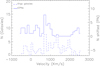 |
Fig. 4. Comparison between the combined ICPN LOSVD constructed in Sect. 2 (continuous blue line) and the LOSVD of the galaxies in the Virgo subcluster A region within 2 deg of M 87 (dashed blue line; (Binggeli et al. 1985, 1987). The ICPN histogram is shifted up by ΔN = 7 for clarity. The lack of ICPN velocites in the M 87 halo range of velocities 1100 km s−1 < VLOS < 2000 km s−1 is related to the lack of information in this range to statistically assign PNs to the ICL component (see Sect. 2.3.2). A K–S test in the velocity range VLOS ≤ 1100 km s−1 returns a probability of 97% that the ICPN LOSVD is drawn from the same distribution as that of the Virgo galaxies. |
2.3.3. PNLF and spatial density profiles of the ICL and the M 87 halo
In this section we describe the effect of the reclassification of the νII ≃ 900 km s−1 component as ICL on the PN luminosity function (PNLF) and on the number density distributions of the M 87 halo PNs and ICPNs.
Longobardi et al. (2015a) showed that their kinematically separated halo PN and IC PN populations had different PNLFs. The IC PNLF differs from the M 87 halo PNLF by having a small value of the c2 parameter in the generalised PNLF formula (Longobardi et al. 2013) and by the presence of a morphological signature denoted as a “dip” located about 1 − 1.5 magnitudes below the bright cut-off of the PNLF. PN population studies relate the presence of this dip to recent star formation (Jacoby & De Marco 2002; Ciardullo et al. 2004; Hernández-Martínez & Peña 2009; Reid & Parker 2010; Ciardullo 2010). The recent work of Gesicki et al. (2018) showed that this dip appears in the PNLF for predominantly opaque nebulae in intermediate stages of expansion.
In M 87 we find that once the νII ≃ 900 km s−1 component is removed, the halo PNLF no longer shows any sign of a dip (see Fig. 5). In this figure, the empirical PNLF is shown together with the fit of the generalised analytic formula for the PNLF, with the bright cut-off at 26.3 magnitude and c2 = 0.72. When the 24 PNs from the νII ≃ 900 km s−1 component and the four kinematic outliers (see Sect. 2.2) are merged with the previously identified ICPN sample from Longobardi et al. (2015a), the IC PNLF dip has higher statistical significance than the earlier analysis (lower panel of Fig. 5). We conclude that the morphology of the PNLFs thus provides independent support to the classification of the νII ≃ 900 km s−1 component as part of the ICL.
We conclude this section by comparing the revised number density profiles of the M 87 halo and IC PNs with the surface brightness profiles of M 87 (see Fig. 6). The IC PN profile now has a slightly steeper gradient than previously quantified by Longobardi et al. (2013); longobardi15a, but it remains shallower than that of the M 87 halo PNs. It is fitted by a power law IICL ∝ R−α with αICL = 0.79 ± 0.15, so it is not consistent with a flat distribution.
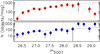 |
Fig. 5. Top: luminosity function of the M 87 halo PNs (red circles) together with the fit of the generalised analytic formula to the halo PNLF, with c2 = 0.72 and bright cut-off at magnitude 26.3. After the statistical subtraction of the reassessed ICL component no residual of a dip is seen. Bottom: PNLF for the ICPNs (blue circles). The blue line shows the fit of the generalised analytic formula to the ICPNLF, with c2 = 0.66 and bright cut-off magnitude at 26.3. The statistical significance of the dip at 1−1.5 mag fainter than the bright cut-off is enhanced compared to Longobardi et al. (2015a). |
2.4. Summary: LOSVD for the M 87 smooth halo
On the basis of the robust sigma and the GMM analysis in this section, we identified the PN outliers and PNs associated with either the revised ICL component or the crown substructure. Each PN velocity measurement then comes with a probability of belonging to the M 87 smooth halo. Thus, we can determine the first (velocity) and second (velocity dispersion) moment of the LOSVD in different regions of the sky and build the corresponding 2D maps. These are the goals of the next section.
3. Two-dimensional kinematics of the M 87 smooth halo: ordered vs. random motions
3.1. Two-dimensional average velocity map
In this section we investigate the average properties of the PN kinematics of the M 87 smooth halo. We build a probability weighted 2D average velocity field using an adaptive Gaussian kernel that matches the spatial resolution to the local density of measurements (Coccato et al. 2009), and weights each PN velocity by the membership probability Γi that the PN belongs to the M 87 smooth halo component (see Sect. 2).
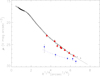 |
Fig. 6. Number density profiles for the M 87 halo PNs (red triangles) and revised ICPNs (blue triangles). The ICPN profile is described by a power-law profile IICL ∝ R−α with αICL = 0.79 ± 0.15 (blue dash-dotted line). As in Longobardi et al. (2015a) it is shallower than the halo PN profile, which closely follows the surface brightness profile of M 87 (black crosses and continuous black line from Kormendy et al. (2009) except in the very outer regions. |
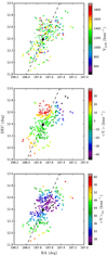 |
Fig. 7. Top: spatial distribution of the 298 spectroscopically confirmed PNs in the halo of M 87, colour-coded according to their VLOS and their size scaled according to their probability of belonging to the smooth halo. The centre of M 87 is shown by the black circle, and the photometric major axis of the galaxy by the dashed line. Middle: smoothed mean velocity field for M 87 using the probability weighted Kernel average of the PNs. Bottom: errors on the smooth velocity map computed by means of Monte Carlo simulations. The mean velocity map indicates that the kinematics is characterised by ordered motion along the galaxy’s major axis. The large positive velocities north-east of M 87 without counterparts in the south-west are likely due to the presence of several PNs with large (∼2σ) velocities relative to M 87 (see text). North is up, east to the left. |
At the position of each source (xP, yP) the mean velocity and velocity dispersion are
 (2)
(2)
and
![Mathematical equation: $$ \begin{aligned} {<}{\sigma }(x_{P},{ y}_{P}){>} =\left[\frac{\sum _{i}{{V_{\mathrm{LOS},i}^2}{ w}_{P,i}}}{\sum _{i}{{ w}_{P,i}}}-{<}{V}(x_{P},{ y}_{P}){>}^2-\Delta V^{2}\right]^{1/2}, \end{aligned} $$](/articles/aa/full_html/2018/12/aa32729-18/aa32729-18-eq10.gif) (3)
(3)
where VLOS, i is the ith PN LOSV and ΔV is the instrumental error, given by the median uncertainty on the velocity measurements, i.e. ΔV = 4.2 km s−1; wP, i is the ith PN weight given by
 (4)
(4)
where Di is the distance of the ith PN to (xP, yP), and k is the amplitude of the kernel. Following Coccato et al. (2009), k is defined to be dependent on the local density of the tracers, ρ(x, y), via
 (5)
(5)
with M = 20 representing the number of nearest neighbours considered in the smoothing technique. A and B are chosen by processing simulated sets of PNs for a given density, velocity gradient, and velocity dispersion as inferred from the data. The simulations returned the following values for A = 0.25 and B = 20.4 kpc. Thus, each PN is assigned a weight which depends on the distance, on the amplitude of the kernel (in turn depending on the local tracer’s number density4), and on its probability of belonging to the M 87 smooth halo component. As described in Coccato et al. (2009, 2013), we can also associate errors on the derived smoothed velocity field by generating 100 different data sets of mock radial velocities with the same positions on the sky as for the real sample of PNs. As the same smoothing procedure is applied to the synthetic data, the statistics of these simulated velocity fields give us the error associated with the smoothed velocity values at the PN positions in our field.
In Fig. 7, we plot the positions of the M 87 halo PNs on the sky, colour-coded on the basis of their LOSV values. The sizes of their symbols are proportional to their probability, Γi, of belonging to the M 87 smooth halo (large symbols; instead, tiny symbols are used for ICPNs). The resulting mean velocity field is given in the central panel. The galaxy’s inner regions are dominated by random motion, with the mean velocity centred on the systemic velocity of M 87, 1307 km s−1. At large radii the system becomes more complex. There are ordered motions along the photometric major axis, with approaching velocities to the north-west, and receding velocities to the south-east side of M 87. Large velocity values are also measured in the north-east regions, without any symmetric counterpart to the south-west.
From Fig. 7 (central panel), it is clear that the amplitude of the ordered motions along the major axis is small, of the order of ∼30 km s−1. This value is within the level of uncertainties, as shown by the error map in the bottom panel of Fig. 7). However, because of its symmetric properties, we consider it real, and it is further analysed in the next section.
The smooth velocity values ∼30 km s−1 obtained to the north-east of M 87 are also consistent with zero, given the uncertainties. As they appear only on one side of the galaxy, this suggests that here we are measuring a local velocity perturbation driven by the presence of a few high-velocity PNs at ∼1800 km s−1 (about 2σ from the systemic velocity of M 87).
3.2. Does the M 87 outer halo rotate?
The amplitude and axis of rotation are evaluated by approximating the mean velocity field with that of an axisymmetric rotator. In that case the mean velocities are modelled by a cosine function of the form
![Mathematical equation: $$ \begin{aligned} {<}\nu _{\rm fit}{>}({\mathrm{PA} },R)=\nu _{\rm sys}(R)+\nu _{\rm cos}(R)\mathrm{cos}[{\mathrm{PA} -\mathrm{PA} _{\rm kin}}(R)], \end{aligned} $$](/articles/aa/full_html/2018/12/aa32729-18/aa32729-18-eq13.gif) (6)
(6)
where R is the major axis distance of each PN from the galaxy’s centre, PA its position angle on the sky (Cohen & Ryzhov 1997). The fitted values νsys, νcos, and PAkin represent the M 87 systemic velocity, the amplitude of the ordered motion, and the kinematic PA, with errors derived from fit uncertainties. To identify possible kinematic decoupling, we divide our PN sample into three elliptical bins: R ≤ 43.8 kpc, 43.8 < R ≤ 73.0 kpc, and R ≥ 73.0 kpc, and Eq. (6) is the fit in each elliptical bin separately. As shown in Fig. 8, left panel, and Table 3, the fitted systemic velocities have values consistent with νsys = 1307.0 ± 7 km s−1 (Allison et al. 2014), with no dependence of the systemic velocity on major axis distance. Instead, the cosine term increases: for R > 73 kpc the cosine component is νcos = 26.76±7.05 km s−1, and PAkin = 161.43°±10.64°. With the photometric major axis at PAphot ≃ 154.4° (Kormendy et al. 2009)5, the kinematic and photometric axes are aligned to within the errors.
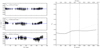 |
Fig. 8. Left: LOS velocities as a function of the PA on the sky for three different elliptical bins (from top to bottom) covering major axis distances in the range R ≤ 43.8 kpc, 43.8 < R ≤ 73.0 kpc, and R ≥ 73.0 kpc. The continuous blue line shows the best-fit model to the data (Eq. (6)), consistent with a system that shows increasing importance of ordered motion with increasing distance, as shown in the plot. The uncertainties on the mean velocities are computed by means of Monte Carlo simulations. Right: cumulative radial λR profile for the halo of M 87 extracted from PN kinematics. The vertical dotted lines identify the major axis distance bins used in the left panel. The black continuous line shows the λ(R) profile computed when approximating the mean velocity field with the best-fit cosine model (blue lines in the left panels), while the grey dash-dotted line shows λ(R) computed from the smoothed velocity data points. At larger radii its amplitude is significantly higher than that of the best-fit cosine model, due to the fluctuations of the mean velocity values around the systemic velocity (see text for details). |
3.3. Cumulative specific angular momentum λR of the M 87 halo
On the basis of the complete 2D velocity information, Emsellem et al. (2007) introduced the λR parameter as a proxy for the projected specific angular momentum of the stars, defined as
 (7)
(7)
where Fi is the flux associated with the ith point, and < V> and < σ> are defined in Eqs. (2) and (3). The λR parameter measures the significance of rotation as a function of the distance from the galaxy’s centre. Galaxies are then classified as fast rotators, λR ≥ 0.1 (nearly axisymmetric systems with aligned photometric and kinematic axes, with a rising λR profile), and slow rotators, λR < 0.1 (nearly round massive galaxies with a significant misalignment between photometric and kinematic axes, moderate degree of triaxiality, and a flat or decreasing λR profile).
We use the probability weighted averaged 2D velocity and velocity dispersion fields to compute the PN λR profile in the surveyed area of the M 87 halo. In line with Coccato et al. (2009), the weighting factor Fi is replaced by 1/cR when summing over the PNs. Here the spatial completeness factor cR is taken from Longobardi et al. (2015a). As discussed by Coccato et al. (2009), this procedure incorporates the weighting by the local stellar surface density by computing a number-weighted sum. In Fig. 7, we show the resulting λR profile for major axis distances in the range 10 kpc ≲ R ≲ 140 kpc for the M 87 halo. The profile is almost flat in the inner ∼70 kpc, and then slowly increases to values of ∼0.11, thus touching the fast-rotators regime (dot-dashed line in Fig. 7, right panel).
To assess the cause for this increase in λR, we compare the observed λR parameter from the 2D field with that computed using the cosine fit from Eq. (6), with νsys, νcos, and PAkin given in Fig. 8 (left panel). As shown in Fig. 8 (right panel, black continuous line), the transition from the inner to the outer regions is still signalled by an increase in the λR profile with major axis distance. However it flattens at a value of λR ∼ 0.05 and never reaches the 0.1 threshold. This difference is driven by the fact that the cosine fit does not represent the apparent streaming velocity in the north of M 87 which we argued above comes from a few high-velocity PNs with velocities ∼1800 km s−16.
Previous studies found that slow rotator galaxies typically increased their rotation from the central regions in their halos, with some entering the regime λR > 0.10 (Coccato et al. 2009; Arnold et al. 2014; Pulsoni et al. 2018). In the case of M 87 the λR parameter also rises in the halo, but only to values λR ≃ 0.05, remaining safely in the slow rotator regime.
4. Velocity dispersion profile of the stellar tracers in M 87
PNs are single stars whose velocities are a discrete realisation of the LOSVD of the stellar population in a given region of a galaxy. PNs are ubiquitous probes of the kinematics of the parent stars at radii where the surface brightness is too faint to measure absorption line features with the required S/N. Hence they are very well suited to complement the stellar-kinematic measurements in the inner regions. In this section, we combine measurements of the second moment of the LOSVD, σ, from absorption line kinematics in the inner high surface brightness regions with those from the PN LOSVDs at large radii, obtaining the velocity dispersion profile out to ∼170 kpc along the major axis. We also discuss velocity dispersion measurements for the GC and UCD systems in M 87 in comparison with the composite σ profile of the stars.
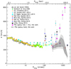 |
Fig. 9. Velocity dispersion profile for the halo of M 87 as function of the average ellipse radius, Ravg = (ab)1/2 of the isophote (for R > 400″ we have assumed a constant ellipticity of e = 0.4). In the inner 80″ = 5 kpc, we show the absorption line data from van der Marel (1994; squares), Sembach & Tonry (1996; green diamonds), and from Emsellem et al. (2014; orange diamonds). Cyan triangles present IFS VIRUS-P data from Murphy et al. (2011, 2014), for the case when the velocity dispersion is computed making use of the entire spectral region (filled triangles) or when it is calculated only from the Mg b region (large open triangles). The yellow shaded area indicates our fiducial velocity dispersion profile of the stars from absorption line spectroscopy (long slit/IFS) in the radial range out to ∼200″ = 15 kpc. The magenta full dots show the new PN velocity dispersion values for our whole sample, i.e. without separation between M 87 halo PNs and ICPNs. The fiducial range of σ estimates we obtain for the M 87 smooth halo PNs alone is indicated by the dark grey area, with boundaries given by the robust estimates of sigma (black line) and by the simple RMS of the halo PN data (dashed black line). The light grey area includes the respective 1σ uncertainties for these values added as well. Thus, the PN kinematics trace a σ profile for the M 87 halo with a strong radial dependence, increasing from 20 to 90 kpc and then decreasing strongly, reaching a minimum value of ∼100 km s−1 at Rav ≃ 130 kpc (Rmaj ≃ 170 kpc). For comparison, red and blue stars show GC velocity dispersion data from Agnello et al. (2014), while black asterisks, and blue and red crosses indicate sample velocity dispersions for UCDs, and blue and red GCs, respectively, as presented in Zhang et al. (2015). |
4.1. Sigma profile within a 20 kpc radius in M 87
M 87 has been the target of many spectroscopic studies with the goal of determining the integrated mass profile from the inner regions to the outermost radii. Velocity dispersion measurements from absorption line spectroscopy (long slits and IFS) available in the literature are reproduced in Fig. 9). In this figure, the velocity dispersion profile of the stars in M 87 is plotted as function of the isophotal average ellipse radius, Ravg = (ab)1/2, where a and b are the isophote major and minor axes.
At Ravg ≤ 5 kpc, the absorption line measurements from van der Marel (1994); Sembach & Tonry (1996) and Emsellem et al. (2014) show a characteristic profile for hot stellar systems. It has a central peak at σ ∼ 400 km s−1, then declines to a value of σ ∼ 270 km s−1 at ∼2 kpc and remains flat out to ∼10 kpc. At these radii the σ measurements from the literature agree within their uncertainties; however, we note that the values from Sembach & Tonry (1996) were corrected for a 7−10% systematic velocity offset attributed by the authors to the large slit width adopted for their observations (for more details see discussion in Sembach & Tonry 1996; Romanowsky & Kochanek 2001; Doherty et al. 2009).
In addition to the MUSE IFS data (Emsellem et al. 2014), VIRUS-P IFS data from Murphy et al. (2011) are also available in this region. At R > 1 kpc, the IFS VIRUS-P measurements have a systematic positive offset of ∼30 km s−1 with respect to the MUSE and slit data. This offset is present when the σ measurements are obtained from the combined analysis of four wavelength regions (G-band, H-beta, Mg b, iron; filled cyan triangles in Fig. 9). When σ values are measured only in the Mg b region of the spectrum (Murphy et al. 2011, open cyan triangles in Fig. 9), then the VIRUS-P and MUSE data sets agree. Then the IFS VIRUS-P measurements (Murphy et al. 2011, open cyan triangles) extend the σ(R) profiles to larger radii. In the radial range 5 kpc < Ravg < 20 kpc, they signal an increase in the velocity dispersion values to ∼280 km s−1.
At radial distances 10 kpc < Ravg < 20 kpc, GCs and UCD galaxies have also been identified and their LOSVDs measured. Red and blue GC sample velocity dispersions from Agnello et al. (2014) and Zhang et al. (2015) are shown as red and blue crosses and plus symbols, respectively. While the σ values of the red GCs are in better agreement with those from the stars (within the uncertainties), blue GC σ values deviate sharply. The velocity dispersion values for the population of Virgo UCDs (black asterisks; Zhang et al. 2015, see Sect. 5 for more discussion) are similar to those of the blue GCs except for the outermost point, which is closer to the red GC dispersion.
4.2. Velocity dispersion profile of the smooth M 87 halo from 20 kpc out to 170 kpc
In Sect. 2 we investigated the influence of the ICL on the PN LOSVDs at radii R > 20 kpc. In the IFS VIRUS-P data, the presence of the ICL is disclosed by the sudden increase in σ from ∼300 km s−1 to nearly ∼600 km s−1 (Murphy et al. 2014 7). The comparison of these values with the running dispersion of the M 87 PN LOSV sample in Fig. 1 shows very good agreement. We note that, because the ICL is unrelaxed (Longobardi et al. 2015a), these high σ values include a significant contribution from unmixed orbital motions and do not trace the enclosed mass only. Therefore, for a proper mass analysis of the M 87 halo, the ICL contribution must be subtracted.
In the course of the extensive analysis carried out in Sect. 2, we computed the probability that each PN is associated with the smooth M 87 halo; we can thus use this probability to compute the histograms of the PN LOSVD for the smooth M 87 halo only, in different outer radial bins. These histograms are shown in Appendix A). They have limited statistics and may thus deviate from Gaussian LOSVDs. To characterise the associated uncertainties, we computed the velocity dispersion values using the robust sigma algorithm8 and the direct RMS values from the PN LOSVDs in these bins. The estimated radii and velocity dispersions using either method are listed in Table 4 for all bins. For small samples the robust sigma may underestimate the true velocity dispersion due to overclipping, and the direct RMS sigma may overestimate it due to its sensitivity to velocities in the wings of the distribution, and so we take these two determinations as the boundaries of our fiducial range of velocity dispersion values from the PN LOSVDs for the smooth M 87 halo. This range is shown by the dark shaded area in Fig. 9, with the lower boundary from the robust sigma depicted by the black continuum line and the RMS estimates by the dashed line, respectively. The range of velocity dispersions obtained by also adding the 1 × σ uncertainties of the two determinations is shown as a light grey shaded area.
Velocity dispersion estimates for the smooth M 87 halo as a function of the major axis distance.
Our fiducial range of velocity dispersion values for the smooth M 87 halo indicates a strong variation in the σ(R) profile with radius. The σ(R) profile from PN LOSVDs extend the slowly rising trend captured by the IFS measurements (Murphy et al. 2014) out to Ravg ≃ 17 kpc, with σ rising to about 280 km s−1 there. The fiducial velocity dispersion range from PNs indicates a further rise in the dispersion to σ ≃ 300 km s−1 at 50 < Ravg < 70 kpc, followed by a steep decline to σ = 100 km s−1, at Ravg ∼ 135 kpc (corresponding major axis radii are 1.3 times larger). We note that the rise and steep drop of the PN velocity dispersion profile is seen on both the NE and SW sides of M 87 (see Fig. 1).
In the next section we investigate whether this strong radial variation in the velocity dispersion profile is consistent with a change in the physical properties of the stellar orbits in these outer regions in dynamical equilibrium. We approach this problem with an approximate analysis based on the spherical Jeans equations, connecting the circular velocity curve inferred from X-ray observations with the surface brightness profile for the smooth M 87 halo.
4.3. Gravitational potential, density, and orbital anisotropy in the outermost halo of M 87
Studies using stellar kinematics, lensing, and X-ray observations (see e.g. Gerhard et al. 2001; Treu et al. 2006; Gavazzi et al. 2007; Churazov et al. 2010) have indicated that the gravitational potentials of elliptical galaxies are approximately isothermal. With this assumption, i.e. that the circular velocity νc is constant, Churazov et al. (2010) showed that the spherical Jeans equation leads to simple relations between νc, the LOS velocity dispersion profile σ(R), and the surface brightness profile I(R). For the case of a system with either isotropic or radial orbital distribution, the relations between νc and the local properties of σ(R) and I(R) are
 (8)
(8)
where α and η are the negative of the logarithmic radial gradients of I(R) and σ(R), and δ is the second logarithmic derivative of I(R)σ2(R); see Eqs. (22, 23) in Churazov et al. (2010) for further detail. Churazov et al. (2010) used the above equations to infer the circular velocity νc,opt from the optical data I(R) and velocity dispersion profile σ(R) at different radii, and for comparison with the circular velocity curve νc,X derived from X-ray emissivity and temperature maps for M 87 from Chandra and XMM-Newton). Their analysis led to a best-fit relation between these two estimates of νc,opt ∼1.10−1.15νc,X, implying an average contribution by non-thermal pressure of 20–30% for six X-ray bright galaxies, with a particularly large value for M 87.
Given our new assessment of the M 87 outer halo kinematics, we carried out an independent comparison of the total enclosed mass profiles from a dynamical estimate using optical data, and from the most recent X-ray information obtained by combining that data of Churazov et al. (2010) with those of Simionescu et al. (2017) at larger radii. Our approach is the following. We adopt the circular velocity curve from the X-ray maps out to 2500 arcsec, and predict the LOS σ(R) profile from the surface brightness distribution of the smooth and relaxed stellar halo of M 87 using Eq. (8). We derive the expected velocity dispersion curves in the isotropic and completely radially anisotropy cases with the goal of comparing with our fiducial σ(R) profile that combines absorption line kinematics with the PN LOS velocity dispersion for the smooth M 87 halo component.
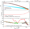 |
Fig. 10. Velocity dispersion profile out to 2000 arcsec compared with predictions from Jeans equations. Panel A: surface brightness profile of the M 87 smooth halo (red crosses and shaded area) obtained from the extended photometry (Kormendy et al. 2009), after subtracting the ICL contribution (blue line and shaded area). The black continuous line shows the Sersic fit with n = 11 to the M 87 halo+ICL extended photometry. The adopted circular velocity profile is shown in panel B. This is a combination of a flat profile (red line) out to 200″ and an increasing profile for larger distances (dashed red line, see text for more information). Panel C: velocity dispersion profile σ(R) from this work (data points, fiducial range from PNs, and legend as in Fig. 9). Large dots represent the expected σ values computed from Eq. (8) at the average radii of the radial bins, for isotropic (orange) and completely radial (red) orbital anisotropy. The comparison with the fiducial range of σ values for halo PNs (shaded area) suggests that the distribution of orbits changes from near-isotropic at ∼200″ to strongly radial at ∼2000″. |
Results are shown in Fig. 10. In panel A, we show the surface brightness profile of the M 87 smooth halo, indicated by the red crosses and red shaded area, the latter indicating the 1σ uncertainty. This surface brightness profile is computed from the extended photometry of M 87 in Kormendy et al. (2009) (black crosses, with continuous black line showing the Sersic fit with n ∼ 11) by subtracting off the ICL contribution (blue line and light blue shaded area, the latter indicating its 1σ uncertainty). The contribution from the ICL was determined in Sect. 2.3.2 and Fig. 6 from the kinematical tagging of the ICPNs. As the inferred ICL surface brightness is of the same order as the surface brightness of the M 87 smooth halo at these large distances, it must be taken into account, i.e. subtracted, so as to have a consistent set of tracer profiles in the Jeans analysis. We note that this analysis cannot be performed for the combined halo plus ICL, because the LOSVD of the ICL shows that it is not in equilibrium in the gravitational potential. Because of the extended tails of its LOSVD, it would lead us to incorrectly infer masses that are too high at the largest radii.
The adopted νc = νc,X is plotted in Panel B. It is a combination of three parts: (i) a flat profile out to 200″ (∼15 kpc) fitted to the data from Churazov et al. (2010); (ii) an increasing profile obtained after differentiating a smooth non-linear fit to the same M 87 X-ray potential data in the range from 200″ (∼15 kpc) to 1200″ (88 kpc), as presented in Churazov et al. (2010, their Fig. 1); and (iii) from 1200″ onward, the circular velocity corresponding to the NFW profile fitted by Simionescu et al. (2017) to their Suzaku data within 400 kpc. The obtained νc = νc,X profile summarises the observational evidence that the circular velocity rises more steeply than an isothermal profile at large radii. We can nonetheless use the local Eq. (8) with this circular velocity profile to estimate velocity dispersions, because νc,X varies only slowly with radius as is confirmed by panel B considering the logarithmic radius scale.
Panel C then shows the expected velocity dispersions σiso and σrad according to Eq. (8), overplotted on the observed M 87 sigma profile as presented in Fig. 9. The comparison between these velocity dispersion estimates and our fiducial velocity dispersion profile suggests that the distribution of orbits in the outer halo of M 87 changes from near-isotropic at 200″ (∼15 kpc) to completely radial at 2300″ (∼170 kpc). The radial velocity dispersion curve inferred from Eq. (8) has non-negligible uncertainties because of the errors in the ICL-subtracted brightness profile and further dynamical modelling will thus be needed to confirm this. We note that because such a dynamical structure of the M 87 halo appears consistent with all data in Fig. 10, it obviates the need for a truncation of the halo density as inferred by Doherty et al. (2009). This is ultimately due to the better statistics in the new ICPN data which allowed us to subtract the (non-equilibrium) ICL component from both the surface brightness and LOS velocity dispersion data.
5. Discussion
5.1. The Virgo ICL: an unrelaxed component in the cluster core
In Sect. 2, we carried out a careful analysis of the PN LOSVs in the velocity range 500−2000 km s−1 around M 87. We identified a velocity component at νII ≃ 900 km s−1 and two pairs of outliers as ICPNs. The complete LOSVD for the ICPN population was then obtained by combining the newly identified 28 ICPNs with those in the extended velocity wings from Longobardi et al. (2015a). The resulting ICPN LOSVD around M 87 has a peak at νII ≃ 900 km s−1 with extended wings, skewed towards negative velocities (Fig. 4).
The identification of the additional 28 ICPNs was supported independently by the increased statistical significance of the dip in the ICL PNLF, and led to improved constraints on the spatial distribution of the ICL thanks to better spatial coverage and statistics. The ICL radial surface density distribution is now consistent with a power law IICL ∝ R−α, with αICL = 0.79 ± 0.15, which is shallower than the Sersic profile for the smooth M 87 halo. The different PNLFs and spatial distributions confirm and strengthen the assessment by Longobardi et al. (2015a) that the M 87 halo and ICL are distinct components. We note that the transition from M 87 to ICL is relatively sudden both in surface brightness and in kinematics (LOSVD). Such sharp transitions are not expected in relaxed clusters. For example, around M 49 in the Virgo subcluster B, the BCG plus IGL system displays a continuous radial transition in both kinematics and stellar population properties (Hartke et al. 2018).
The dynamical properties of the ICL around M 87 can be used as a benchmark for advanced hydrodynamical simulations of galaxy clusters. The separation of central galaxy (M 87) and ICL on the basis of different LOSVDs has similar aspects as the classification as function of binding energy of stellar particles in simulated cluster centres (Dolag et al. 2010; Cui et al. 2014). Stars with high binding energies come from mergers of fairly massive progenitors, i.e. relaxation and merging processes that led to rapid changes in the gravitational potential. As a result these particles have lost memory of their progenitors, while particles with low binding energies still reflect the dynamics of their lower mass satellite progenitors. In particle tagging methods (Cooper et al. 2015) BCGs and ICL have thus been associated with relaxed/unrelaxed accreted components.
The Illustris TNG simulations (Pillepich et al. 2018) made detailed predictions on ICL fractions and spatial distributions that can be compared with the results from the current investigation. In what follows we assume a total halo mass of ≃3 × 10¹⁴ M⊙ for the Virgo cluster (Karachentsev & Nasonova 2010). For this halo mass, the Illustris TNG simulations predict a best-fitting power-law slope of −αTNG,ICL ∼ −2.2 to the 2D stellar mass surface density of the combined halo and ICL. In the outer regions of M 87 (R < 150 kpc) we measure −α ≃ −(2.0−2.5), in approximate agreement. The ICL alone has a shallower radial profile there, −αICL ≃ −0.8.
For the Virgo cluster halo mass, the simulations predict approximate ICL stellar mass fractions out to the virial radius of ∼0.35 for an aperture > 30 kpc, and of ∼0.2 for an aperture > 100 kpc (Pillepich et al. 2018, their Fig. 10). From Longobardi et al. (2015a), in the radial range 7 kpc < R < 150 kpc the V-band luminosities of the M 87 halo and ICL are Lhalo = 4.42 × 10¹⁰ L⊙ and LICL = 0.53 × 10¹⁰ L⊙, respectively9. For the M/L ratios, γ*, we adopt values assigned by the colour-mass-to-light ratio (McGaugh & Schombert 2014), using the B − V colours measured for the outer halo and ICL, respectively. For the M 87 outer halo, we adopt  for a colour of B − V = 0.76, as in Longobardi et al. (2015b); for the ICL,
  for a colour B − V ∼ 0.6 measured at 130 kpc from the centre of M 87 (Mihos et al. 2017). These luminosities and M/L ratios result in a stellar mass fraction of 0.05 for the ICL for R < 150 kpc around M 87. This appears lower than the predicted values, but the comparison depends on how quickly the slope of the ICL density steepens outside our observed range.
The Illustris TNG simulations also make predictions on the minimum progenitor stellar mass, such that satellites of this mass and higher contribute 90% of the total ex situ stellar mass around BCGs. For the B − V ∼ 0.6 colour of the M 87+ICL light at 130 kpc distance (Mihos et al. 2017) and a 10 Gyr old stellar population, the metallicity is [Fe/H] ≤ −1.0. This agrees with the results of Williams et al. (2007) who found from HST data in a Virgo ICL field that about 70–80% of the stars have ages > 10 Gyr and mean metallicity −1.0. Using the stellar mass metallicity relation (Zahid et al. 2017), we can infer the progenitor stellar mass for these stars, resulting in a few ×108 M⊙. In contrast, Fig. 13 from Pillepich et al. (2018) predicts larger progenitor masses of a few ×109 M⊙. The reason for this discrepancy is probably not related to the young dynamical age of the Virgo cluster core inferred from its unrelaxed velocity distribution (see Sect. 2 and Fig. 4). While in this case the effective mass of the accreting M 87 subcluster might be a few times lower than the Virgo cluster virial mass, the predicted minimum progenitor masses are insensitive to such variations. A more likely possibility is that the simulations miss a population of lower-mass galaxies (Hartke et al. 2018).
5.2. Smooth halo as tracer of the gravitational potential in M 87: comparison between optical and X-ray circular velocity curves
After subtracting the strongly non-Gaussian ICL LOSVD, and the LOSVD of the crown substructure, the remaining smooth M 87 halo has kinematics centred on the galaxy’s systemic velocity (1307 km s−1) and characterised by approximately Gaussian LOSVDs (see Sect. 2 and Appendix A). Mean rotation velocities in the halo are ≲25 km s−1 (Sect. 3), and the velocity dispersion profile, after rising slowly to σ ≃ 300 km s−1 at Ravg ≃ 50−70 kpc, then declines steeply down to σ = 100 km s−1 at Ravg ∼ 135 kpc (Sect. 4; corresponding major axis radii are 1.3 times larger).
By smooth halo we mean the part of the halo that is approximately phase-mixed (i.e. has approximately Gaussian LOSVDs centred about the systemic velocity), at the resolution of our PN survey. This is in contrast to the ICL component around M 87, which is obviously non-Gaussian (Fig. 4), and to the more localised phase-space substructure identified as the crown (Longobardi et al. 2015b). However, because of the likely accretion origin of also the smooth outer halo, and the long associated phase mixing timescales at R ∼ 100 kpc, we expect that this component too would show lower mass or amplitude substructures if it were possible to look at its phase-space with a much larger number of stellar tracers. Nonetheless the working concept of the smooth halo is useful because the approximately Gaussian LOSVDs enable us to determine well-defined velocity dispersions and tracer densities for carrying out a Jeans analysis of the mass and anisotropy at large radii.
M 87 is an X-ray bright elliptical galaxy and the gravitational potential can be traced directly by modelling the hot gas atmosphere, under the assumption of hydrostatic equilibrium (e.g. Nulsen & Bohringer 1995). However, the comparison between the circular speed profiles computed from dynamical modelling of the stars’ LOS velocities and from the X-ray data in several nearby massive ellipticals including M 87 has indicated that the depth of the potential well derived from the X-ray emitting hot gas is systematically lower than the corresponding optical value (from stars) such that νc, opt = η × νc, X with η = 1.10−1.14-pagination (Churazov et al. 2010). This implies that the mass estimates from X-ray data underestimate the enclosed total mass by 21%–30%, and has been considered as evidence for a significant non-thermal pressure support (Churazov et al. 2008; Gebhardt & Thomas 2009; Shen & Gebhardt 2010; Das et al. 2010).
Nonetheless we were able in Sect. 4.3 to obtain a consistent interpretation of the tracer density and velocity dispersion profile of the smooth halo in the gravitational potential obtained from the X-ray data of Churazov et al. (2010) and Simionescu et al. (2017). Using the local, spherically symmetric Jeans analysis method of Churazov et al. (2010) we found that the radial variation in the LOS dispersion profile σ(Ravg), rising from 270 to 300 km s−1 in the radial range 10 kpc ≤ Ravg ≤ 70 kpc followed by a decline to 100 km s−1 at Ravg = 135 kpc, can be reproduced by an isotropic stellar orbital distribution in the radial range up to ∼60 kpc, which becomes strongly radially anisotropic outside 70–135 kpc. The strong decline at the largest radii is similar to what is measured in our own Milky Way halo (see Fig. 15 in Bland-Hawthorn & Gerhard 2016). The strong radial dependence of σ(Ravg) for the smooth M 87 halo can be generated from a flat and then rising νc, X, a steeper I(R) for the smooth M 87 halo, as shown in panels A and B of Fig. 10, and a varying orbital anisotropy profile with radial dependence indicated in panel C of Fig. 10). This simplified picture provides a consistent description of the velocity dispersion profile for the smooth M 87 halo, and sets the basis for a more sophisticated dynamical model to follow.
We also computed the predicted σICL profile from the X-ray circular velocity profile νc, X and the full Sersic profile (n = 11 including the ICL; from K09) for an isotropic orbital distribution. Even with an increasing circular speed and a flatter surface brightness profile the predicted σ(Ravg) at 135 kpc is ∼540 km s−1, i.e. it does not rise fast enough to reproduce the upward σ profile obtained when the ICL PNs are included (magenta full dots in Fig. 9). This is due to the non-Gaussian ICL LOSVD, and supports previous assessments that the ICL around M 87 is not (or not yet) in dynamical equilibrium.
We note that the modelling of the smooth halo indicates very strong radial anisotropy at the outermost radii probed by the PN data. This suggests that if the hydrostatic interpretation of the X-ray data significantly underestimated the M 87 circular velocity curve at ∼100 kpc radius, it would be difficult to find a dynamical equilibrium model matching the low dispersion there. Thus, non-thermal pressure contributions may in fact be small at those radii, and the hydrostatic pressure of the X-ray emitting gas therefore traces the enclosed mass. We also note that the new modelling obviates the need for a truncation of the density inferred by Doherty et al. (2009) because the new velocity dispersion profile and surface density profile of the smooth halo appear consistent with the mass distribution from X-rays. This is ultimately due to the better statistics in the new ICPN data which allowed us to subtract the (non-equilibrium) ICL component from both the surface brightness and LOS velocity dispersion data.
5.3. M 87 kinematics as traced by GCs and ultra-compact dwarfs
In addition to PNs, GCs and UCDs are used as bright tracers to measure LOSVs and thus overcome the limits represented by the very low surface brightnesses characteristic of the outer regions of the M 87 halo. It is of interest then to compare the results from the different tracers in order to assess any similarities or discrepancies, and to understand the origin of the latter.
Strader et al. (2011) presented a detailed kinematic analysis10 of a sample of ∼400 GC LOSVs that covers the M 87 halo out to 40′ (∼175 kpc). They found that all the GC populations are characterised by rotation that becomes stronger at large radii. However GC subsamples with different average colours have rotation that differs both in amplitude and direction.
By comparing Strader et al. (2011) results to the PN kinematics of the M 87 smooth halo presented in this study, we found differences that are most significant with respect to the kinematics of the metal-poor GC subsample. The fiducial velocity dispersion profile of the smooth M 87 halo as traced by the stars and PNs is in broad agreement with the red GC population, within the uncertainties (see also Fig. 9). Unlike the red GCs subsample though, the PN velocity field for the M 87 smooth halo did not show any signatures of rotation along the photometric minor axis (see discussion in Sect. 3). For distances larger than 10′, the bluer GC population and the M 87 smooth halo PNs are rotating about the galaxy’s photometric minor axis, with the former having a larger amplitude of rotation.
The different kinematics shown by the different GC populations may be related to a Virgo ICGC population in addition to a M 87 GC halo population. Durrell et al. (2014) provided evidence for a Virgo ICGC populations on the basis of an excess of number counts in the Virgo core within the extended area surveyed by the Next Generation Virgo Cluster Survey. Both Durrell et al. (2014) and Ko et al. (2017) found an ICGC population mostly associated with blue GCs. This is consistent with results from simulations (e.g. Ramos et al. 2015), who showed that galaxies moving into Virgo-like clusters are stripped mainly of their blue GC component (see also Longobardi et al. 2018, for the first definitive kinematic detection of the ICGC population in the Virgo cluster). We can then speculate that the more metal-poor GCs contain a large fraction of IC population with its distinct kinematics. It is interesting to note that the LOSVD associated with the “green” GCs, as identified by Strader et al. (2011), shows a secondary peak in their distribution (see Fig. 23 in their work) similar to what has been identified as the νII ∼ 900 km s−1 component in the PN M 87 halo sample, and later associated with the Virgo ICL in Sect. 2). If there is a fraction of red ICGCs, we expect it to be lower.
A more recent study presented by Zhang et al. (2015) analysed the properties of a sample of UCD galaxies within 2 square degrees centred on M 87, and compared it to the properties of the red and blue GC population. Their results show that the surface number density profile of the UCDs is shallower than that of the blue GC sample in the inner 15′ and becomes as steep as the red GC component at larger radii. Moreover, they showed that the entire UCD system presents a larger amplitude rotation than the GCs, with a rotational axis that is more aligned with the red GC population in the same radial range. These results show that the UCD system around M 87 is kinematically distinct from the GC population, and also from the M 87 halo PNs. The presence of distinct populations of tracers with multi-spins and different kinematics can be understood in terms of an extended mass assembly of the M 87 halo. Tidal interactions and different specific frequencies of the tracers, depending on the progenitor satellites galaxies, can explain the occurrence of the kinematical diversity in the halo of bright ellipticals like M 87 (Coccato et al. 2013).
6. Conclusions
In this work we analysed the kinematics of 298 PNs in the outer regions of M 87, covering the galaxy halo and intra-cluster stars out to average radius Ravg∼ 135 kpc (corresponding to ∼170 kpc along the major axis). Our main results are the following:
-
(i)
Including a newly identified νII ≃ 900 km s−1 component, the intra-cluster stars have a strongly non-Gaussian LOSVD with a peak at that velocity, and strong, asymmetric wings. The shape of the LOSVD is consistent with the LOSVD of the galaxies in the Virgo subcluster A, and indicates that the ICL stars around M 87 as well as the subcluster A galaxies are not (yet) in dynamical equilibrium, signalling the on-going build-up of the Virgo cluster.
-
(ii)
The so-called dip in the intra-cluster PN luminosity function has strengthened with respect to earlier analyses, while no dip is seen in the PNLF of the M 87 halo. This independently supports the kinematic classification of the PNs into halo and ICL. The surface density profile of the kinematically tagged ICPNs decreases as a power law with radius, with negative logarithmic slope −αICL = −0.79 ± 0.15 in this region.
-
(iii)
Based on the previously published B − V colour (Mihos et al. 2017) and on resolved HST photometry (Williams et al. 2007), the metallicity of the ICL population is estimated as [Fe/H] ≃ −1.0. This suggests masses of a few ×108 M⊙ for the ICL progenitor galaxies, which is an order of magnitude less massive than the predictions from the Illustris TNG simulation (Pillepich et al. 2018).
-
(iv)
The PNs in the smooth M 87 halo, i.e. the part of the halo which is approximately phase-mixed at the resolution of our PN survey, thus have a somewhat steeper surface density profile than the total surface brightness profile from Kormendy et al. (2009) for halo and ICL together. The rotation of these stars in the outer halo is small, ≲25 km s−1, safely in the slow rotator regime. The velocity dispersion profile of the smooth halo PNs rises slowly from the σ ≃ 270 km s−1 at ≃2−10 kpc seen in integrated spectra to σ ≃ 300 ± 50 km s−1 at average ellipse radii Ravg ≃ 50−70 kpc, but then declines steeply down to σ = 100 km s−1 at Ravg ∼ 135 kpc.
-
(v)
Simple dynamical models indicate that the surface density and velocity dispersion profiles of the smooth halo PN tracers at these large radii are consistent with being in approximate dynamical equilibrium in the gravitational potential inferred from hydrostatic analysis of the X-ray emitting gas. The X-ray circular velocity curve rises steeply outside ∼30 kpc, reaching νc,X ∼ 700 km s−1 at 200 kpc. This requires a change in the anisotropy of the halo stellar orbits from an approximately isotropic distribution in the radial range up to ∼60 kpc to a strongly radially anisotropic configuration at the largest radii probed, Ravg = 135 kpc, as would be expected if the outer halo was accreted from infalling satellites.
Compared to Longobardi et al. (2015a) (254), one repeated object has been discarded.
These quantities represent the mean velocity and velocity dispersion of subsequences of n adjacent PN velocities along the major axis. Here n = 30.
The kernel size is 80 km s−1, corresponding approximately to σM 87/4, where σM 87 = 298.4 km s−1 is the velocity dispersion associated with the M 87 halo from the robust procedure in Longobardi et al. (2015a). This kernel size represents a compromise between faithful structure representation and noise smoothing.
See Coccato et al. (2009) for a full description of the smoothing technique.
PA is measured with respect the north axis, with east to the left.
This increase in the λR profile from fluctuations in the mean velocity field is different from that described in Wu et al. (2014) which results from fluctuations in the velocity distribution around the local mean velocity.
In that paper, dispersion values are computed using the information coming from the entire spectral region between 4100 Å–5400 Å.
For a short description of this technique see Appendix A. More details can be found in Longobardi et al. (2015a).
These luminosities account for the fraction of ICPNs in the range of velocities covered by the M 87 halo.
Strader et al. (2011) compute an extended comparison with previously published GC samples, and we refer the reader to their work for further information.
Acknowledgments
AL thanks Jonathan N. Elliott for advice and suggestions on the manuscript and Guido Avvisati who helped in the installation of IDL libraries. OG thanks Natalya Lyskova and Eugene Churazov for discussions on the M 87 X-ray potential. AL acknowledges the China Postdoc Foundation’s fund 2017M610693. AL and MAR wish to acknowledge ESO support via the Science Support Discretionary Funds 18/28. This research has made use of the NASA/IPAC Extragalactic Database (NED) which is operated by the Jet Propulsion Laboratory, California Institute of Technology, under contract with the National Aeronautics and Space Administration.
References
- Agnello, A., Evans, N. W., Romanowsky, A. J., & Brodie, J. P. 2014, MNRAS, 442, 3299 [NASA ADS] [CrossRef] [Google Scholar]
- Allison, J. R., Sadler, E. M., & Meekin, A. M. 2014, MNRAS, 440, 696 [NASA ADS] [CrossRef] [Google Scholar]
- Arnaboldi, M., Gerhard, O., Aguerri, J. A. L., et al. 2004, ApJ, 614, L33 [NASA ADS] [CrossRef] [Google Scholar]
- Arnold, J. A., Romanowsky, A. J., Brodie, J. P., et al. 2014, ApJ, 791, 80 [NASA ADS] [CrossRef] [Google Scholar]
- Barbosa, C. E., Arnaboldi, M., Coccato, L., et al. 2018, A&A, 609, A78 [NASA ADS] [CrossRef] [EDP Sciences] [Google Scholar]
- Bender, R., Saglia, R. P., & Gerhard, O. E. 1994, MNRAS, 269, 785 [NASA ADS] [CrossRef] [Google Scholar]
- Bender, R., Kormendy, J., Cornell, M. E., & Fisher, D. B. 2015, ApJ, 807, 56 [NASA ADS] [CrossRef] [Google Scholar]
- Binggeli, B., Sandage, A., & Tammann, G. A. 1985, AJ, 90, 1681 [NASA ADS] [CrossRef] [Google Scholar]
- Binggeli, B., Tammann, G. A., & Sandage, A. 1987, AJ, 94, 251 [NASA ADS] [CrossRef] [Google Scholar]
- Bland-Hawthorn, J., & Gerhard, O. 2016, ARA&A, 54, 529 [NASA ADS] [CrossRef] [EDP Sciences] [Google Scholar]
- Bullock, J. S., & Johnston, K. V. 2005, ApJ, 635, 931 [NASA ADS] [CrossRef] [Google Scholar]
- Churazov, E., Forman, W., Vikhlinin, A., et al. 2008, MNRAS, 388, 1062 [NASA ADS] [CrossRef] [Google Scholar]
- Churazov, E., Tremaine, S., Forman, W., et al. 2010, MNRAS, 404, 1165 [NASA ADS] [Google Scholar]
- Ciardullo, R. 2010, PASA, 27, 149 [NASA ADS] [Google Scholar]
- Ciardullo, R., Durrell, P. R., Laychak, M. B., et al. 2004, ApJ, 614, 167 [Google Scholar]
- Cimatti, A., Nipoti, C., & Cassata, P. 2012, MNRAS, 422, L62 [NASA ADS] [CrossRef] [Google Scholar]
- Coccato, L., Gerhard, O., Arnaboldi, M., et al. 2009, MNRAS, 394, 1249 [NASA ADS] [CrossRef] [Google Scholar]
- Coccato, L., Arnaboldi, M., & Gerhard, O. 2013, MNRAS, 436, 1322 [NASA ADS] [CrossRef] [Google Scholar]
- Cohen, J. G., & Ryzhov, A. 1997, ApJ, 486, 230 [NASA ADS] [CrossRef] [Google Scholar]
- Conselice, C. J., Gallagher, III., J. S., & Wyse, R. F. G. 2001, ApJ, 559, 791 [NASA ADS] [CrossRef] [Google Scholar]
- Cook, B. A., Conroy, C., Pillepich, A., Rodriguez-Gomez, V., & Hernquist, L. 2016, ApJ, 833, 158 [NASA ADS] [CrossRef] [Google Scholar]
- Cooper, A. P., Gao, L., Guo, Q., et al. 2015, MNRAS, 451, 2703 [NASA ADS] [CrossRef] [Google Scholar]
- Cortesi, A., Arnaboldi, M., Coccato, L., et al. 2013, A&A, 549, A115 [NASA ADS] [CrossRef] [EDP Sciences] [Google Scholar]
- Côté, P., McLaughlin, D. E., Hanes, D. A., et al. 2001, ApJ, 559, 828 [NASA ADS] [CrossRef] [Google Scholar]
- Cui, W., Murante, G., Monaco, P., et al. 2014, MNRAS, 437, 816 [NASA ADS] [CrossRef] [Google Scholar]
- Das, P., Gerhard, O., Churazov, E., & Zhuravleva, I. 2010, MNRAS, 409, 1362 [NASA ADS] [CrossRef] [Google Scholar]
- Doherty, M., Arnaboldi, M., Das, P., et al. 2009, A&A, 502, 771 [NASA ADS] [CrossRef] [EDP Sciences] [Google Scholar]
- Dolag, K., Murante, G., & Borgani, S. 2010, MNRAS, 405, 1544 [NASA ADS] [Google Scholar]
- Dopita, M. A., Jacoby, G. H., & Vassiliadis, E. 1992, ApJ, 389, 27 [NASA ADS] [CrossRef] [Google Scholar]
- D’Souza, R., Kauffman, G., Wang, J., & Vegetti, S. 2014, MNRAS, 443, 1433 [NASA ADS] [CrossRef] [Google Scholar]
- Durrell, P. R., Côté, P., Peng, E. W., et al. 2014, ApJ, 794, 103 [NASA ADS] [CrossRef] [Google Scholar]
- Emsellem, E., Cappellari, M., Peletier, R. F., et al. 2004, MNRAS, 352, 721 [NASA ADS] [CrossRef] [Google Scholar]
- Emsellem, E., Cappellari, M., Krajnović, D., et al. 2007, MNRAS, 379, 401 [NASA ADS] [CrossRef] [Google Scholar]
- Emsellem, E., Krajnović, D., & Sarzi, M. 2014, MNRAS, 445, L79 [NASA ADS] [CrossRef] [Google Scholar]
- Forman, W., Jones, C., & Tucker, W. 1985, ApJ, 293, 102 [NASA ADS] [CrossRef] [Google Scholar]
- Gavazzi, R., Treu, T., Rhodes, J. D., et al. 2007, ApJ, 667, 176 [NASA ADS] [CrossRef] [Google Scholar]
- Gebhardt, K., & Thomas, J. 2009, ApJ, 700, 1690 [NASA ADS] [CrossRef] [Google Scholar]
- Gebhardt, K., Adams, J., Richstone, D., et al. 2011, ApJ, 729, 119 [NASA ADS] [CrossRef] [Google Scholar]
- Gerhard, O. E. 1993, MNRAS, 265, 213 [NASA ADS] [CrossRef] [Google Scholar]
- Gerhard, O., Kronawitter, A., Saglia, R. P., & Bender, R. 2001, AJ, 121, 1936 [NASA ADS] [CrossRef] [Google Scholar]
- Gerhard, O., Arnaboldi, M., Freeman, K. C., et al. 2005, ApJ, 621, L93 [NASA ADS] [CrossRef] [Google Scholar]
- Gesicki, K., Zijlstra, A. A., & Miller Bertolami, M. M. 2018, Nat. Astron., 2, 580 [NASA ADS] [CrossRef] [Google Scholar]
- Gonzalez, A. H., Zaritsky, D., & Zabludoff, A. I. 2007, ApJ, 666, 147 [NASA ADS] [CrossRef] [Google Scholar]
- Hartke, J., Arnaboldi, M., Longobardi, A., et al. 2017, A&A, 603, A104 [NASA ADS] [CrossRef] [EDP Sciences] [Google Scholar]
- Hartke, J., Arnaboldi, M., Gerhard, O., et al. 2018, A&A, 616, A123 [NASA ADS] [CrossRef] [EDP Sciences] [Google Scholar]
- Hernández-Martínez, L., & Peña, M. 2009, A&A, 495, 447 [NASA ADS] [CrossRef] [EDP Sciences] [Google Scholar]
- Hernquist, L., & Barnes, J. E. 1991, Nature, 354, 210 [NASA ADS] [CrossRef] [Google Scholar]
- Hoffman, L., Cox, T. J., Dutta, S., & Hernquist, L. 2010, ApJ, 723, 818 [NASA ADS] [CrossRef] [Google Scholar]
- Huang, S., Ho, L. C., Peng, C. Y., Li, Z.-Y., & Barth, A. J. 2013, ApJ, 768, L28 [NASA ADS] [CrossRef] [Google Scholar]
- Hui, X., Ford, H. C., Ciardullo, R., & Jacoby, G. H. 1993, ApJ, 414, 463 [NASA ADS] [CrossRef] [Google Scholar]
- Jacoby, G. H., & De Marco, O. 2002, AJ, 123, 269 [Google Scholar]
- Janowiecki, S., Mihos, J. C., Harding, P., et al. 2010, ApJ, 715, 972 [NASA ADS] [CrossRef] [Google Scholar]
- Karachentsev, I. D., & Nasonova, O. G. 2010, MNRAS, 405, 1075 [NASA ADS] [Google Scholar]
- Ko, Y., Hwang, H. S., Lee, M. G., et al. 2017, ApJ, 835, 212 [NASA ADS] [CrossRef] [Google Scholar]
- Kormendy, J., Fisher, D. B., Cornell, M. E., & Bender, R. 2009, ApJS, 182, 216 [NASA ADS] [CrossRef] [Google Scholar]
- Longobardi, A., Arnaboldi, M., Gerhard, O., et al. 2013, A&A, 558, A42 [NASA ADS] [CrossRef] [EDP Sciences] [Google Scholar]
- Longobardi, A., Arnaboldi, M., Gerhard, O., & Hanuschik, R. 2015a, A&A, 579, A135 [NASA ADS] [CrossRef] [EDP Sciences] [Google Scholar]
- Longobardi, A., Arnaboldi, M., Gerhard, O., & Mihos, J. C. 2015b, A&A, 579, L3 [NASA ADS] [CrossRef] [EDP Sciences] [Google Scholar]
- Longobardi, A., Peng, E. W., Côté, P., et al. 2018, ApJ, 864, 36 [NASA ADS] [CrossRef] [Google Scholar]
- McGaugh, S. S., & Schombert, J. M. 2014, AJ, 148, 77 [NASA ADS] [CrossRef] [Google Scholar]
- McNeil, E. K., Arnaboldi, M., Freeman, K. C., et al. 2010, A&A, 518, A44 [NASA ADS] [CrossRef] [EDP Sciences] [Google Scholar]
- McNeil-Moylan, E. K., Freeman, K. C., Arnaboldi, M., & Gerhard, O. E. 2012, A&A, 539, A11 [NASA ADS] [CrossRef] [EDP Sciences] [Google Scholar]
- Mei, S., Blakeslee, J. P., Côté, P., et al. 2007, ApJ, 655, 144 [NASA ADS] [CrossRef] [Google Scholar]
- Méndez, R. H., Riffeser, A., Kudritzki, R.-P., et al. 2001, ApJ, 563, 135 [NASA ADS] [CrossRef] [Google Scholar]
- Mihos, J. C., Harding, P., Feldmeier, J. J., et al. 2017, ApJ, 834, 16 [NASA ADS] [CrossRef] [Google Scholar]
- Murphy, J. D., Gebhardt, K., & Adams, J. J. 2011, ApJ, 729, 129 [NASA ADS] [CrossRef] [Google Scholar]
- Murphy, J. D., Gebhardt, K., & Cradit, M. 2014, ApJ, 785, 143 [NASA ADS] [CrossRef] [Google Scholar]
- Nulsen, P. E. J., & Bohringer, H. 1995, MNRAS, 274, 1093 [NASA ADS] [Google Scholar]
- Oser, L., Ostriker, J. P., Naab, T., Johansson, P. H., & Burkert, A. 2010, ApJ, 725, 2312 [NASA ADS] [CrossRef] [Google Scholar]
- Oser, L., Naab, T., Ostriker, J. P., & Johansson, P. H. 2012, ApJ, 744, 63 [NASA ADS] [CrossRef] [Google Scholar]
- Pedregosa, F., Varoquaux, G., Gramfort, A., et al. 2011, J. Mach. Learn. Res., 12, 2825 [Google Scholar]
- Peng, E. W., Ford, H. C., & Freeman, K. C. 2004, ApJ, 602, 685 [NASA ADS] [CrossRef] [Google Scholar]
- Pillepich, A., Nelson, D., Hernquist, L., et al. 2018, MNRAS, 475, 648 [NASA ADS] [CrossRef] [Google Scholar]
- Pota, V., Forbes, D. A., Romanowsky, A. J., et al. 2013, MNRAS, 428, 389 [NASA ADS] [CrossRef] [Google Scholar]
- Pulsoni, C., Gerhard, O., Arnaboldi, M., et al. 2018, ArXiv e-prints [arXiv:1712.05833] [Google Scholar]
- Ramos, F., Coenda, V., Muriel, H., & Abadi, M. 2015, ApJ, 806, 242 [NASA ADS] [CrossRef] [Google Scholar]
- Reid, W. A., & Parker, Q. A. 2010, MNRAS, 405, 1349 [NASA ADS] [Google Scholar]
- Romanowsky, A. J., & Kochanek, C. S. 2001, ApJ, 553, 722 [NASA ADS] [CrossRef] [Google Scholar]
- Romanowsky, A. J., Strader, J., Brodie, J. P., et al. 2012, ApJ, 748, 29 [NASA ADS] [CrossRef] [Google Scholar]
- Schindler, S., & Boehringer, H. 1993, A&A, 269, 83 [NASA ADS] [Google Scholar]
- Schuberth, Y., Richtler, T., Hilker, M., et al. 2010, A&A, 513, A52 [NASA ADS] [CrossRef] [EDP Sciences] [Google Scholar]
- Sembach, K. R., & Tonry, J. L. 1996, AJ, 112, 797 [NASA ADS] [CrossRef] [Google Scholar]
- Shen, J., & Gebhardt, K. 2010, ApJ, 711, 484 [NASA ADS] [CrossRef] [Google Scholar]
- Simionescu, A., Werner, N., Mantz, A., Allen, S. W., & Urban, O. 2017, MNRAS, 469, 1476 [NASA ADS] [CrossRef] [Google Scholar]
- Spavone, M., Capaccioli, M., Napolitano, N. R., et al. 2017, A&A, 603, A38 [NASA ADS] [CrossRef] [EDP Sciences] [Google Scholar]
- Strader, J., Romanowsky, A. J., Brodie, J. P., et al. 2011, ApJS, 197, 33 [NASA ADS] [CrossRef] [EDP Sciences] [Google Scholar]
- Tal, T., & van Dokkum, P. G. 2011, ApJ, 731, 89 [NASA ADS] [CrossRef] [Google Scholar]
- Thomas, D., Maraston, C., Bender, R., & Mendes de Oliveira, C. 2005, ApJ, 621, 673 [NASA ADS] [CrossRef] [Google Scholar]
- Treu, T., Koopmans, L. V., Bolton, A. S., Burles, S., & Moustakas, L. A. 2006, ApJ, 640, 662 [NASA ADS] [CrossRef] [Google Scholar]
- van der Marel, R. P. 1994, MNRAS, 270, 271 [NASA ADS] [CrossRef] [Google Scholar]
- van Dokkum, P. G., Whitaker, K. E., Brammer, G., et al. 2010, ApJ, 709, 1018 [NASA ADS] [CrossRef] [Google Scholar]
- Ventimiglia, G., Arnaboldi, M., & Gerhard, O. 2011, A&A, 528, A24 [NASA ADS] [CrossRef] [EDP Sciences] [Google Scholar]
- Williams, B. F., Ciardullo, R., Durrell, P. R., et al. 2007, ApJ, 656, 756 [NASA ADS] [CrossRef] [Google Scholar]
- Wu, X., Gerhard, O., Naab, T., et al. 2014, MNRAS, 438, 2701 [NASA ADS] [CrossRef] [Google Scholar]
- Zahid, H. J., Kudritzki, R.-P., Conroy, C., Andrews, B., & Ho, I.-T. 2017, ApJ, 847, 18 [NASA ADS] [CrossRef] [Google Scholar]
- Zhang, H.-X., Peng, E. W., Côté, P., et al. 2015, ApJ, 802, 30 [NASA ADS] [CrossRef] [Google Scholar]
- Zibetti, S., White, S. D. M., Schneider, D. P., & Brinkmann, J. 2005, MNRAS, 358, 949 [Google Scholar]
- Zhu, L., Long, R. J., Mao, S., et al. 2014, ApJ, 792, 59 [NASA ADS] [CrossRef] [Google Scholar]
Appendix A: LOSVD of the M 87 outer regions
This appendix provides additional information on the fiducial σ profile and its dependencies on the uncertainties associated with (i) the identification of the ICL stars in the range of velocities associated with the M 87 halo, (ii) limited number statistics, and (iii) deviations of the LOSVD in radial bins from a Gaussian distribution. In Fig. A1, we show the PN LOSVDs in six radial bins; they are those adopted in Fig. 9 and the ΔR is indicated on the top of each panel. In each panel, we illustrate the modification of the LOSVDs, depending on the application of the different constraints.
 |
Fig. A.1. Planetary nebula LOSVDs in six radial bins from the M 87 centre; the radial range is displayed above each panel. In each panel, the histogram limited by the black continuous line shows the LOSVD of the M 87 halo PNs as classified in Longobardi et al. (2015a). The histogram limited by the continuous red line shows the PN LOSVDs of the smooth M 87 halo once the νII ≃ 900 km s−1 component is accounted for. For smooth M 87 halo PN LOSVDs we further plot two Gaussians, one with mean and dispersion computed as simple mean and standard deviation of the LOSV data (green continuous line), and another whose mean and dispersion value computed from the robust estimator (McNeil et al. 2010; Longobardi et al. 2015a, blue continuous line), and (2). The red shaded histogram shows the PN LOSVDs once the robust estimator is applied. We note that in the fourth and fifth radial bin the velocity dispersion estimates deviate the most because of the deviation of LOSVDs from a Gaussian and the limited statistics. |
In each panel, we plot the histogram of the PN LOSVD associated with the M 87 halo by Longobardi et al. (2015a) with the black continuous line; the histogram delimited by the red continuous line is computed for the PN LOSVs without the νII ≃ 900 km s−1 component, and represents the smooth M 87 halo. The PN LOSVDs clearly deviate from a straight Gaussian distribution and are affected by limited number statistics in the outermost bins. Hence we proceed to estimate the second moment of the PN LOSVDs for the smooth M 87 halo as a fiducial range, whose limits are given by the values obtained from the standard deviation from the measured LOSVs (upper limit) and from a robust sigma estimate from the LOSVD (lower limit).
In each panel, we show two Gaussian profiles, one with mean and dispersion values obtained from a robust procedure (blue continuous line), and the other with mean and dispersion computed as simple mean and standard deviation of the LOSVs in the bin (green continuous line). The value obtained from the robust estimate is computed according to McNeil et al. (2010) and Longobardi et al. (2015a). The red shaded histogram presents the PN LOSVDs selected by appling the robust estimator in each bin.
The range of values for the second moment of the PN LOSVDs associated with the smooth M 87 halo in the different radial bins is shown in Fig. 9 as a grey shaded area function of the distance, and represents our fiducial velocity dispersion profile.
Appendix B: PN catalogue
Here we present the M 87 PN catalogue obtained from the PN photometric and spectroscopic surveys carried out with Suprime-Cam mounted on the Subaru Telescope and the FLAMES spectrograph installed on the VLT, respectively, and presented in Longobardi et al. (2013); longobardi15a. In this catalogue we provide the PN coordinates (J2000 system), the [OIII]λ5007 Å magnitudes, and heliocentric VLOS measured from a Gaussian fit to the [OIII]λ5007Å emission. In high S/N spectra, we also detect the redshifted [OIII] λ4959/5007 Å doublet. Typical S/N for the spectroscopically confirmed PN [OIII]]λ5007 Å cover a range of 2.5 ≲ S/N ≲ 15.0 per resolution element. From the repeated observations of the same candidates in different FLAMES plate configurations we estimated the median deviation of velocity measurements to be 4.2 km s−1, and that the hole distribution covers a range of 0.6 < ΔV < 16.2 km s−1. In the case of repeated observations the given heliocentric velocity has been estimated from the spectrum with the highest S/N. Longobardi et al. (2015a) discussed a statistical approach to determine the fraction of misclassified PNs based on the analysis of stacked PN spectra. They determined that 2% of the entire sample (seven PNs) could represent misclassified spectra (for more details see Longobardi et al. 2015a).
The table is divided into three parts: (i) PNs that have a higher probability of belonging to the smooth halo component and PNs that have a high probability of belonging to the crown structure (indicated by *; Longobardi et al. 2015b), (ii) PNs that have a higher probability of belonging to the additional ICL component as determined in this work (see Sect. 2) and (iii) PNS that have been assigned to the ICL component by Longobardi et al. (2015a). This table is only available in electronic form at the CDS.
All Tables
Gaussian fitting parameters from the GMM decomposition of the M 87 halo PN LOSVD for the subsamples along the minor axis, major axis north, and major axis south.
Velocity dispersion estimates for the smooth M 87 halo as a function of the major axis distance.
All Figures
|
Fig. 1. Left: projected phase-space diagram VLOS vs. major axis distance R from the centre of M 87 out to 200 kpc for all spectroscopically confirmed PNs from Longobardi et al. (2015a); their M 87 halo PNs (red asterisks) and ICPNs (blue asterisks) are shown separately; R > 0 and R < 0 represent the northern and southern halves with respect the galaxy centre. Red open circles show four newly identified kinematic outliers (see Sect. 2.2). Black dash-dotted and black continuous lines depict the running average and running velocity dispersion independently for the M 87 south-east and north-west, computed from the 253 halo PNs. Full red circles show the robust estimate of the halo velocity dispersion following Longobardi et al. (2015a), while full black circles show the velocity dispersion values after probability-weighted removal of the crown substructure from Longobardi et al. (2015b). Both velocity dispersion profiles (red and black circles) show strong radial variation, with a steep decline at major axis distances R > 100 kpc. Green dash-dotted and green continuous lines show the running average and velocity dispersion for the combined sample of 253 halo PNs and 45 ICPNs; the inclusion of ICPNs leads to a rapidly rising velocity dispersion profile. Cyan triangles show the velocity dispersion measurements from the IFU VIRUS-P data of Murphy et al. (2011, 2014) whose outer rise near R = 700″ (∼40 kpc) is matched by the running joint halo and ICPN velocity dispersion (green line) indicative of the contribution from the ICL. Right: zoomed-in plot in the velocity range ±1000 km s−1 centred on the systemic velocity of M 87. |
| In the text | |
|
Fig. 2. Generalised histogram for (i) the entire M 87 halo PN LOSVD (top left), (ii) the subsample along the minor axis (top right), and (iii) the subsample along the major axis north (bottom left) and (iv) south (bottom right) of M 87. The PNs for each subsample are depicted in red in the spatial distributions shown in the top right corner of each panel. All histograms show a multi-peaked distribution, with a secondary peak at ∼1000 km s−1. The probability that such a secondary peak is caused by low number statistics is ∼18% (see text for details). |
| In the text | |
|
Fig. 3. Histograms of the LOSVD along the M 87 major (top four panels) and minor axis (bottom centre panel). The larger number of tracers associated with the M 87 halo allows us to divide the halo PN sample into northern (top left panels) and southern (top right panels) subsamples; moreover, the PN subsamples along the major axis are further divided in two elliptical bins, as given in the panels. The best-fit GM model (thick black line) identifies in all subsamples two Gaussian components (green lines). Dashed histograms represent the PN LOSVD prior to the statistical subtraction of the crown substructure. |
| In the text | |
|
Fig. 4. Comparison between the combined ICPN LOSVD constructed in Sect. 2 (continuous blue line) and the LOSVD of the galaxies in the Virgo subcluster A region within 2 deg of M 87 (dashed blue line; (Binggeli et al. 1985, 1987). The ICPN histogram is shifted up by ΔN = 7 for clarity. The lack of ICPN velocites in the M 87 halo range of velocities 1100 km s−1 < VLOS < 2000 km s−1 is related to the lack of information in this range to statistically assign PNs to the ICL component (see Sect. 2.3.2). A K–S test in the velocity range VLOS ≤ 1100 km s−1 returns a probability of 97% that the ICPN LOSVD is drawn from the same distribution as that of the Virgo galaxies. |
| In the text | |
|
Fig. 5. Top: luminosity function of the M 87 halo PNs (red circles) together with the fit of the generalised analytic formula to the halo PNLF, with c2 = 0.72 and bright cut-off at magnitude 26.3. After the statistical subtraction of the reassessed ICL component no residual of a dip is seen. Bottom: PNLF for the ICPNs (blue circles). The blue line shows the fit of the generalised analytic formula to the ICPNLF, with c2 = 0.66 and bright cut-off magnitude at 26.3. The statistical significance of the dip at 1−1.5 mag fainter than the bright cut-off is enhanced compared to Longobardi et al. (2015a). |
| In the text | |
|
Fig. 6. Number density profiles for the M 87 halo PNs (red triangles) and revised ICPNs (blue triangles). The ICPN profile is described by a power-law profile IICL ∝ R−α with αICL = 0.79 ± 0.15 (blue dash-dotted line). As in Longobardi et al. (2015a) it is shallower than the halo PN profile, which closely follows the surface brightness profile of M 87 (black crosses and continuous black line from Kormendy et al. (2009) except in the very outer regions. |
| In the text | |
|
Fig. 7. Top: spatial distribution of the 298 spectroscopically confirmed PNs in the halo of M 87, colour-coded according to their VLOS and their size scaled according to their probability of belonging to the smooth halo. The centre of M 87 is shown by the black circle, and the photometric major axis of the galaxy by the dashed line. Middle: smoothed mean velocity field for M 87 using the probability weighted Kernel average of the PNs. Bottom: errors on the smooth velocity map computed by means of Monte Carlo simulations. The mean velocity map indicates that the kinematics is characterised by ordered motion along the galaxy’s major axis. The large positive velocities north-east of M 87 without counterparts in the south-west are likely due to the presence of several PNs with large (∼2σ) velocities relative to M 87 (see text). North is up, east to the left. |
| In the text | |
|
Fig. 8. Left: LOS velocities as a function of the PA on the sky for three different elliptical bins (from top to bottom) covering major axis distances in the range R ≤ 43.8 kpc, 43.8 < R ≤ 73.0 kpc, and R ≥ 73.0 kpc. The continuous blue line shows the best-fit model to the data (Eq. (6)), consistent with a system that shows increasing importance of ordered motion with increasing distance, as shown in the plot. The uncertainties on the mean velocities are computed by means of Monte Carlo simulations. Right: cumulative radial λR profile for the halo of M 87 extracted from PN kinematics. The vertical dotted lines identify the major axis distance bins used in the left panel. The black continuous line shows the λ(R) profile computed when approximating the mean velocity field with the best-fit cosine model (blue lines in the left panels), while the grey dash-dotted line shows λ(R) computed from the smoothed velocity data points. At larger radii its amplitude is significantly higher than that of the best-fit cosine model, due to the fluctuations of the mean velocity values around the systemic velocity (see text for details). |
| In the text | |
|
Fig. 9. Velocity dispersion profile for the halo of M 87 as function of the average ellipse radius, Ravg = (ab)1/2 of the isophote (for R > 400″ we have assumed a constant ellipticity of e = 0.4). In the inner 80″ = 5 kpc, we show the absorption line data from van der Marel (1994; squares), Sembach & Tonry (1996; green diamonds), and from Emsellem et al. (2014; orange diamonds). Cyan triangles present IFS VIRUS-P data from Murphy et al. (2011, 2014), for the case when the velocity dispersion is computed making use of the entire spectral region (filled triangles) or when it is calculated only from the Mg b region (large open triangles). The yellow shaded area indicates our fiducial velocity dispersion profile of the stars from absorption line spectroscopy (long slit/IFS) in the radial range out to ∼200″ = 15 kpc. The magenta full dots show the new PN velocity dispersion values for our whole sample, i.e. without separation between M 87 halo PNs and ICPNs. The fiducial range of σ estimates we obtain for the M 87 smooth halo PNs alone is indicated by the dark grey area, with boundaries given by the robust estimates of sigma (black line) and by the simple RMS of the halo PN data (dashed black line). The light grey area includes the respective 1σ uncertainties for these values added as well. Thus, the PN kinematics trace a σ profile for the M 87 halo with a strong radial dependence, increasing from 20 to 90 kpc and then decreasing strongly, reaching a minimum value of ∼100 km s−1 at Rav ≃ 130 kpc (Rmaj ≃ 170 kpc). For comparison, red and blue stars show GC velocity dispersion data from Agnello et al. (2014), while black asterisks, and blue and red crosses indicate sample velocity dispersions for UCDs, and blue and red GCs, respectively, as presented in Zhang et al. (2015). |
| In the text | |
|
Fig. 10. Velocity dispersion profile out to 2000 arcsec compared with predictions from Jeans equations. Panel A: surface brightness profile of the M 87 smooth halo (red crosses and shaded area) obtained from the extended photometry (Kormendy et al. 2009), after subtracting the ICL contribution (blue line and shaded area). The black continuous line shows the Sersic fit with n = 11 to the M 87 halo+ICL extended photometry. The adopted circular velocity profile is shown in panel B. This is a combination of a flat profile (red line) out to 200″ and an increasing profile for larger distances (dashed red line, see text for more information). Panel C: velocity dispersion profile σ(R) from this work (data points, fiducial range from PNs, and legend as in Fig. 9). Large dots represent the expected σ values computed from Eq. (8) at the average radii of the radial bins, for isotropic (orange) and completely radial (red) orbital anisotropy. The comparison with the fiducial range of σ values for halo PNs (shaded area) suggests that the distribution of orbits changes from near-isotropic at ∼200″ to strongly radial at ∼2000″. |
| In the text | |
|
Fig. A.1. Planetary nebula LOSVDs in six radial bins from the M 87 centre; the radial range is displayed above each panel. In each panel, the histogram limited by the black continuous line shows the LOSVD of the M 87 halo PNs as classified in Longobardi et al. (2015a). The histogram limited by the continuous red line shows the PN LOSVDs of the smooth M 87 halo once the νII ≃ 900 km s−1 component is accounted for. For smooth M 87 halo PN LOSVDs we further plot two Gaussians, one with mean and dispersion computed as simple mean and standard deviation of the LOSV data (green continuous line), and another whose mean and dispersion value computed from the robust estimator (McNeil et al. 2010; Longobardi et al. 2015a, blue continuous line), and (2). The red shaded histogram shows the PN LOSVDs once the robust estimator is applied. We note that in the fourth and fifth radial bin the velocity dispersion estimates deviate the most because of the deviation of LOSVDs from a Gaussian and the limited statistics. |
| In the text | |
Current usage metrics show cumulative count of Article Views (full-text article views including HTML views, PDF and ePub downloads, according to the available data) and Abstracts Views on Vision4Press platform.
Data correspond to usage on the plateform after 2015. The current usage metrics is available 48-96 hours after online publication and is updated daily on week days.
Initial download of the metrics may take a while.