| Issue |
A&A
Volume 619, November 2018
|
|
|---|---|---|
| Article Number | A58 | |
| Number of page(s) | 20 | |
| Section | Interstellar and circumstellar matter | |
| DOI | https://doi.org/10.1051/0004-6361/201833146 | |
| Published online | 06 November 2018 | |
Properties of cold and warm H I gas phases derived from a Gaussian decomposition of HI4PI data
1
Argelander-Institut für Astronomie,
Auf dem Hügel 71,
53121
Bonn,
Germany
e-mail: This email address is being protected from spambots. You need JavaScript enabled to view it.
2
Tartu Observatory, University of Tartu,
61602
Tõravere,
Tartumaa,
Estonia
Received:
2
April
2018
Accepted:
2
June
2018
Abstract
Context. A large fraction of the interstellar medium can be characterized as a multiphase medium. The neutral hydrogen gas is bistable with cold and warm neutral medium (CNM and WNM respectively) but there is evidence for an additional phase at intermediate temperatures, a lukewarm neutral medium (LNM) that is thermally unstable.
Aims. We use all sky data from the HI4PI survey to separate these neutral H I phases with the aim to determine their distribution and phase fractions f in the local interstellar medium.
Methods. HI4PI observations, gridded on an nside = 1024 HEALPix grid, were decomposed into Gaussian components. From the frequency distribution of the velocity dispersions we infer three separate linewidth regimes. Accordingly we extract the H I line emission corresponding to the CNM, LNM, and WNM. We generateed all-sky maps of these phases in the local H I gas with − 8 < vLSR < 8 km s−1.
Results. Each of the H I phases shows distinct structures on all scales. The LNM never exists as a single phase but contributes on average 41% of the H I. The CNM is prominent only for 22% of the sky, contributes there on average 34% but locally up to 60% of the H I and is associated with dust at temperatures Tdust ~ 18.6 K. Embedded cold filaments show a clear anti-correlation between CNM and LNM. Also the smoothly distributed WNM is anti-correlated with the CNM. It contributes for the rest of the sky 39% with dust associated at temperatures Tdust ~ 19.4 K.
Conclusions. The CNM in filaments exists on small scales. Here the observed anti-correlation between LNM and CNM implies that both, filaments and the surrounding more extended LNM, must have a common origin.
Key words: ISM: general / ISM: structure / dust, extinction / ISM: clouds
© ESO 2018
1 Introduction
The interstellar medium, notably the H I, exists as a multiphase medium. Field et al. (1969) pointed out that most of the H I should exist in two stable phases in pressure equilibrium, the cold neutral medium (CNM) at excitation temperatures T < 300 K, and the WNM at T≲104 K. But soon Salpeter (1976), reviewing the formation and destruction of interstellar dust grains, objected and argued that there must be a third unstable phase at intermediate temperatures. This phase was dubbed by him the luke-warm neutral medium (LNM).
McKee & Ostriker (1977) extended the two-phase model of Field et al. (1969) and considered supernova (SN) explosions in an in-homogeneous environment. Their model of the interstellar medium (ISM) has three phases, including the ionized medium, and is dominated by individual SN explosions. The interior of SN remnants is filled by the hot ionized medium (HIM). Blast waves sweep up the gas inside the bubbles and pile it up into the shells. As soon as this gas is shocked, it starts to cool. It recombines rapidly and forms the CNM.
Subsequently the thermal equilibrium gas temperatures of the diffuse interstellar medium were calculated by Wolfire et al. (1995) an updated by Wolfire et al. (2003). These investigations have shown that there can be conditions where the H I gas is thermally unstable. However, the conclusion was that the local ISM is probably only marginally in the regime in which there must be more than two bistable H I phases.
From observations there were early indications for substantial amounts of unstable H I gas. Among others, significant contributions from unstable H I gas were observed by Dickey et al. (1977), Mebold et al. (1982), Kalberla et al. (1985), Spitzer & Fitzpatrick (1995), Fitzpatrick & Spitzer (1997). However, it was Heiles (2001) who initiated a vivid debate with the statement “Large amounts of thermally unstable gas are not allowed in theoretical models of the global interstellar medium”. From the Arecibo absorption line survey toward 79 sources there was evidence that 60% of the gas is WNM. At least 48% of this WNM turned out to be unstable (Heiles & Troland 2003a). In other words, 30% of the gas belongs to the LNM. More recently, Roy et al. (2013) obtained for 33 compact extragalactic radio sources deep high-velocity resolution absorption line data. They found that at least 28% of the gas must have temperatures in the thermally unstable range. A more recent study of H I absorption in the direction of 57 background radio sources with the Very Large Array (Murray et al. 2015) has found an even smaller mass fraction of thermally unstable HI, about 20%.
Subsequent theoretical investigations have shown that considerable amounts of unstable gas can be induced by turbulence. Gazol et al. (2001) conclude that about 50% of the turbulent gas mass has temperatures that are characteristic for the LNM. Audit & Hennebelle (2005) find also large fractions of thermally unstable gas. This fraction increases with the amplitude of the turbulent forcing. The thermally unstable gas tends to be organized in filamentary structures. Similar, de Avillez & Breitschwerdt (2005) find that up to 49% of the mass belongs to the thermally unstable regime. In general, these results show all that turbulence is playing a key role for phase transition in the H I gas (Saury et al. 2014).
The debate about the multiphase composition of the H I gas was summarized by Vázquez-Semadeni (2012) and amounts to the questionwhether classical discrete-phase models need to be replaced by a “phase continuum”. For details we refer to this excellent review.
In this paper we want to study phase dependencies in the local H I gas. We used high resolution observations of the all-sky H I brightness temperature distribution with large single dish radio telescopes. The data are decomposed into Gaussian components. We find three distinct linewidth-regimes that can be considered to represent the CNM, LNM, and WNM. Section 2 describes the observations, the data reduction, the Gaussian decomposition and selection criteria applied by us. Using Gaussian parameters we model separate H I distributions for the CNM, LNM, and WNM. These distributions are presented in Sect. 3 and we discuss the column density distributions in detail. The Sky appears to contain regions thatare dominated by the CNM. In Sect. 4 we separate these regions and discuss phase dependent distributions for column densities and associated dust temperatures. Cold filamentary gas stands out and is discussed in more detail in Sect. 5. The interrelations between H I phases are shown in Sect. 6. Our results are discussed in Sect. 7, the summary is in Sect. 8.
2 Observations and data reduction
2.1 The HI4PI 21-cm line survey
For the northern hemisphere we use the Effelsbeg–Bonn H I Survey (EBHIS) from observations with the 100-m Effelsberg radio telescope (Winkel et al. 2016a,b) and for the southern hemisphere the Galactic All Sky Survey (GASS), observed with the 64 m Parkes telescope (McClure-Griffiths et al. 2009; Kalberla et al. 2010; Kalberla & Haud 2015). Both surveys, EBHIS with the first data release (Winkel et al. 2016b) and GASS with its final data release (Kalberla & Haud 2015), were gridded in position to a common nside = 1024 HEALPix database (Górski et al. 2005). After calibration, this was first step in merging both surveys and initially the original velocity vectors, different for both surveys, were kept. We used this intermediate data product, both surveys with their genuine spatial resolution and original velocity vectors, for our Gaussian decomposition as described in Sect. 2.2. When merging both surveys by HI4PI Collaboration (2016), the EBHIS beam shape was adapted to the GASS resolution. In addition the GASS spectra were smoothed and adapted to the EBHIS velocity grid. In our analysis, to decompose the spectra as accurate as possible into Gaussian components, we stayed as close as possible to the original database but used positions on the common HEALPix grid. To calculate maps for this publication we use Gaussian components to generate profiles on the HEALPix grid. Next the data are smoothed to a common effective resolution of 30′, afterward maps are generated.
Using an nside = 1024 HEALPix database implies an effective angular resolution of Θpix = 3.′44 for that grid (Górski et al. 2005). The EBHIS data were gridded to an effective beam sized with FWHM = 10.′8, and the GASS to FWHM = 16.′2. This means that our database is over-sampled, neighboring positions are not independent from each other. Our choice of the nside = 1024 HEALPix database is motivated by the aim to enable an easy comparison between all-sky H I data and published Planck maps.
The Gaussian analysis enables us to separate different phases according to the linewidth-regimes derived in Sect. 2.3. We generate separate maps for the CNM, LNM, and WNM. The EBHIS and GASS overlap for declinations − 5° < δ < 1°. When selecting Gaussian components we use a border line between both surveys at δ = −2°. To avoid discontinuities in maps, caused by different beam sizes, we used a linear interpolation between both surveys for − 4° < δ < 0°.
2.2 Gaussian analysis
After generating the HEALPix database, we decomposed all brightness temperature spectra Tb (vi) into Gaussian components
![Mathematical equation: \begin{equation*} T_{\mathrm{b}}(v_i) = \sum_{j=1}^N T_{\mathrm{bc,j}} \exp \left[-\frac{(v_i - v_{\mathrm{c},j})^2} {2\sigma_j^2}\right],\end{equation*}](/articles/aa/full_html/2018/11/aa33146-18/aa33146-18-eq1.png) (1)
(1)
where Tbc,j, vc,j, and σj are the adjustable parameters of the Gaussian component j, the sum is taken over N components, describing the given profile and vi is the central velocity of the spectrometer channel i. For the decomposition we used mostly the same approach, which was described by Haud (2000) and applied earlier to the Leiden/Argentine/Bonn (LAB) data (Kalberla et al. 2005). In general, this is a rather classical Gaussian decomposition, but with two important additions, introduced for reducing the ambiguities inherent to the decomposition procedure. First of all, our decomposition algorithm does not treat each H I profile independently, but assumes that every observed profile shares some similarities with those in the neighboring sky positions, as expected for an over-sampled database. In addition, besides adding components into the decomposition, our algorithm also analyzes the results to find the possibilities for removing or merging some Gaussians without reducing too much the accuracy of the representation of the original profile with decomposition. For the acceptable decomposition we required that the RMS of the weighted deviations of the Gaussian model from the observed profile had to be no more than 1.006 times the weighted noise level of the emission-free baseline regions of this profile. This condition corresponds to | lg (χ2∕Ndof)| < 0.015, but we must keep in mind that here both, the estimates of the standard deviations of the data points and the fitted models are based on the same data set. The value of the multiplier has been chosen so that the averages of the noise levels and the RMS deviations of the models over all HEALPix profiles of the survey are equal (in practice, for the final decomposition the difference of these averages was less than 0.09% of their mean).
For the decomposition of the HI4PI, we also introduced some modifications to our old algorithm. First of all, the accuracy of the measured brightness temperatures is not the same for all profile channels. According to the radiometer equation the noise level depends on the signal strength and different corrections applied during the processing of the observed spectral dumps introduce additional uncertainties. During the decomposition, all this was considered through the weights assigned to all values of Tb (vi) of the profile in each HEALPix pixel. For the GASS part of the HI4PI, these weights were calculated from the RMS deviations of the spectral dumps from the corresponding average profile in each pixel, as described in Kalberla & Haud (2015). For EBHIS, the Tsys (vi) together with the RFI flags was used as a proxy for the RMS in the individual spectral dumps contributing to the HEALPix pixel.
As the velocity resolution of the EBHIS data is the lowest among the decomposed surveys, it revealed a problem with the original decomposition algorithm: near the steepest gradients in the observed profiles the decomposition results often contained groups of very high (|Tbc|≫|(Tb(vi) + Tb(vi+1)∕2|), but narrow (σ < Δv, where Δv = vi+1 − vi is the channel separation of the survey) Gaussians, which centers were located between the consecutive spectrometer channels vi and vi+1. The obtained decompositions fitted well the observed profiles at vi and vi+1, but with strong fluctuations between the measured data points. To suppress such a behavior, we used the penalty function approach. During the decomposition, we calculated at vc,j of all Gaussians the deviations of the model from the cubic spline representation of the observed profile and added the weighted squares of these deviations to the RMS of the fit. The weights of these penalty points were calculated as  , where δvmin is the positive velocity difference between the vc,j and the nearest vi. W was obtained from the cubic spline fit of the weights of the observed profile at velocities vc,j.
After finding this problem in the decomposition of the EBHIS, we performed a special search in the results of the GASS decomposition and found similar narrow Gaussians also there. The only difference was that in the GASS such components appeared in general one at a time and therefore did not cause so obvious oscillations of the resulting model profiles as in EBHIS. Nevertheless, in the final decomposition, the modification for suppressing such Gaussians was applied to both the EBHIS and GASS data.
Considerable change in the decomposition algorithm was made available by the increased power of the computers. In the LAB survey, we used the decomposition results of one of the neighboring profiles of any given profile as an initial estimate of the Gaussianparameters, and we only started the decomposition of the first profile with one roughly estimated component at the highest maximum of the profile. In the HI4PI study, the decomposition was divided into two stages. In the first run, we decomposed all profiles in the HEALPix database independently of their neighbors, starting with one Gaussian at the brightest tip of the profile. In the second stage, we compared the results for neighboring profiles. To accomplish this, we used the decomposition obtained so far for each profile as an initial approximation for all eight nearest neighbors of this profile, and checked whether this led to better decomposition of these neighboring profiles. If the decomposition of a neighbor was improved, the new result was used as an initial solution for the eight neighbors of this profile, and so on. The processwas repeated until no more improvements were found (on the order of 500 runs through the full database).
During this process, we estimated the goodness of the obtained fits using two criteria. First of all, as described above, we did not accept the decompositions for which the RMS of the weighted deviations of the Gaussian model from the observed profile exceeded more than 1.006 times the weighted noise level of the emission-free baseline regions of this profile. If for some profiles the RMS criterion was satisfied for more than one trial decomposition with different numbers of Gaussians, we accepted the solution with the smallest number of the components. In the case of acceptable decompositions with equal numbers of the Gaussians, we chose the decomposition with the smallest RMS as the best. The decomposition process is described in more detail in Sects. 3.1 and 3.2 of Haud (2000).
Finally, in the case of the LAB, we only used positive Gaussians (Tbc > 0 K) for decomposition and the parts of the profiles with  were not considered at all. With the HI4PI, we also fitted negative Gaussians to the regions of the profiles where the brightness temperature was on average below zero. For fitting the regions of the profiles, where
  , we still used only positive Gaussians and not a combination of positive and negative components. Therefore, only strong absorption or the baseline problems, where the
  of the profile drops below the continuum level, induced negative Gaussians. In general, absorption was modeled as a gap between positive Gaussians.
2.3 Defining different HI phases
The hypothesis that the H I component line shapes are Gaussian rests on the assumption that motions within any H I cloud have a random velocity distribution that can be described by a Gaussian function. This assumption is supported by the finding that the H I absorption features are often well represented by Gaussians in optical depth τ(ν) (Mohan et al. 2004). The decomposition of the emission profiles is physically meaningful only when τ(ν) ≪ 1. Nevertheless, both the opacity and brightness profiles of most sources are easily decomposed into Gaussians, so whether or not this model is physically correct, it works empirically and is convenient.
As a result, the Gaussian decomposition offers an opportunity to differentiate between components with different line widths (Haud & Kalberla 2007). In combination with absorption-line studies (Dickey et al. 2003; Heiles & Troland 2003a), components with broad or narrow line widths have been found to arise from the WNM and CNM, respectively (Dickey & Lockman 1990; Wolfire et al. 2003; Hennebelle & Falgarone 2012) and there could be substantial amounts of thermally unstable LNM as well (Heiles & Troland 2003a; Haud & Kalberla 2007; Hennebelle & Falgarone 2012; Roy et al. 2013; Saury et al. 2014).
Our decomposition of the full HEALPix database of the HI4PI profiles gave on average 8.472 Gaussians per profile, but the complexity of the profiles greatly varies between different sky regions and often the Gaussians in the decomposition are heavily blended with each other. This considerably complicates the physical interpretation of the results, as for such profiles the decomposition may be not unique. This means that several quite different solutions may approximate the observed profile almost equally well, and the decomposition provides no satisfactory means for choosing between these solutions, while others, equally good or even better ones, may not be found at all. As described in Sect. 2.2, we have tried to reduce this problem by keeping the number of the used Gaussians as low as possible and by considering during the decomposition of each profile the information about the neighboring profiles.
In this way we hope that for similar profiles the algorithm prefers similar decompositions, which may better represent the general properties of the H I gas than the set of more independent solutions. Nevertheless, these precautions cannot guarantee that our decomposition results mostly describe the properties of the underlying H I gas and are not dominated by the random factors inherent to the decomposition process. Therefore, we decided to compare first the results, obtained from independent observations (the LAB vs. HI4PI) with different decomposition algorithms (as described in Sect. 2.2). We expect that the similarity of the results, obtainable from such studies indicate that the main properties of the results are determined by the nature of the galactic gas but in cases where uncertainties in the Gaussian decomposition are dominant the results may yield nearly incomparable outcomes.
It is clear that the blending and non-uniqueness problems are weaker for the simplest profiles and for the strongest Gaussians in the decompositions of the more complicated profiles. Therefore, as with the LAB (Haud & Kalberla 2007), we started the analysis of the HI4PI data with the simplest profiles in the database, which are located at relatively high galactic latitudes and followed the changes in the results caused by gradually adding more complicated profiles at lower latitudes (Fig. 1). With the HI4PI data we used for these tests only the Gaussians which belong to the central peaks of the observed profiles. We defined the central peak as the maximum of Tb (vi) closest to vLSR = 0 km s−1. We considered this peak to extend to the velocities where the Tb(v), calculated from the decomposition results, drops below the noise level of the corresponding observed profile.
This approach had an additional advantage that it eliminated from the analysis nearly all noise Gaussians without applying any formal selection criteria (as Eqs. (3) and (4) in Haud & Kalberla 2007). Only a rather small contamination by RFI remained. In some cases such approach included also intermediate- (IVC) or even high-velocity clouds (HVC) into our sample, but as in the following we will apply also different velocity limits on the studied components, this is not a considerable problem. Moreover, we will use the number of the Gaussians in the central peak of the profiles, NG, as an indicator of the profile complexity and study only the profiles with moderate complexity. As the inclusion of IVCs and HVCs as local gas increases NG for the corresponding pixels, such cases have higher probability to be excluded as too complex profiles. Figure 1 gives the sky distribution of the described complexity estimates for NG < 8.
Using the LAB data, we have demonstrated (Haud & Kalberla 2007) that by considering only the simplest H I profiles and relatively small LSR velocities (− 9 ≤ vc ≤ 4 km s−1) it is possibleto distinguish three groups of preferred line-widths, which are defined by fitting the sum of log-normal functions to the frequency distribution of the Gaussian widths. It is found that on the basis of the LAB profiles decomposed into one, two, or three lowvelocity Gaussians, the estimates for the mean line-widths of the CNM, LNM, and WNM gas are 4.9 ±0.1, 12.0 ± 0.3, and 24.4 ± 0.2 km s−1 (Fig. 4 in Haud & Kalberla (2007)). In the same way, we obtained from the decomposition of the HI4PI survey the values 4.7 ± 0.4, 11.2 ± 0.6, and 24.2 ± 0.4 km s−1 (Fig. 2). For CNM and WNM the results from LAB and HI4PI are rather close to each other. The agreement is slightly worse for the LNM, but this is understandable, as the frequency distribution of the widths of the LNM Gaussians is blended by both, CNM and WNM. This makes the separation of this gas phase more uncertain.
Besides the curves for CNM, LNM, and WNM Fig. 2 (also Fig. 4 in Haud & Kalberla 2007) contains a fourth curve, labeled here as XNM. At first sight, the nature of this component is not obvious and therefore we made a special study of the profiles, responsible for this component (see Appendix A). It turned out that the corresponding Gaussians are weak and in many cases they describe the wide non-Gaussian wings of the profiles, but sometimes (mostly in the EBHIS part of the HI4PI but in less then 3% of all positions) they are caused by instrumental problems. We found from different models that these Gaussians represent 3.2%–5.3% of the total H I and in the following they are considered as belonging to WNM.
In the two lower panels of the Fig. 2 a similar, but even weaker enhancement is visible also on the left edge of the distribution. This is caused by rare and very narrow noise Gaussians, still remaining in the analyzed data sample. As their contribution is very small, we did not use an additional log-normal curve for describing this enhancement and in the following the corresponding Gaussians are considered as part of CNM.
As can be seen from Fig. 2, with increasing complexity of the profiles the relative number of CNM Gaussians increases and up to a certain complexity limit this permits better determination of the parameters of the CNM gas phase from the width distribution of the corresponding Gaussians. However, at considerably higher complexity levels (NG > 10) of the profiles the definition of the LNM phase becomes more and more questionable as the decompositions of the complex profiles usually contain many weak Gaussians with rather ill-defined parameters. Such components add noise to the distribution of the widths of the Gaussians, and the CNM, LNM, and WNM components of the width distribution start to merge into a relatively structureless curve, where the maximum corresponding to LNM is completely blended by CNM and WNM. Therefore, the separation of CNM, LNM, and WNM phases is best determined for the profiles with some moderate complexity.
To estimate the reasonable complexity limit, we analyzed the width distributions of the Gaussians from the profiles with 1 ≤ NG ≤ 15 and found that the uncertainties of the parameters of the LNM phase started to grow more rapidly for NG ≥ 8. As for NG ≤ 3 we obtained for NG ≤ 7 the following mean line-widths of the CNM, LNM, and WNM gas: 3.6 ± 0.1, 9.6 ±1.3, and 23.3 ± 0.6 km s−1. The distribution of the Gaussianwidths for NG ≤ 7 together with the corresponding model curves are given in Fig. 3. The sky distribution of all profiles used for these estimates is in Fig. 1. Despite the fact that here we used a considerably simplified approach to the determination of these averages (we dropped the analysis of the reliability of the decompositions of the profiles with NG ≥ 4, as it was done byHaud & Kalberla 2007), these estimates are comparable with the final results of (Haud & Kalberla 2007; FWHM = 3.9 ± 0.6, 11.8 ± 0.5, and 24.1 ± 0.6 km s−1).
As a result, we may recognize that Gaussian fits to observed H I emission or absorption profiles have been applied by anumber of authors (e.g., Takakubo & van Woerden 1966; Mebold 1972; Mebold et al. 1982; Heiles & Troland 2003b; Nidever et al. 2008; Murray et al. 2015). We have used it with the LAB, GASS, and EBHIS data (Haud & Kalberla 2007; Kalberla & Haud 2015; Kalberla et al. 2016, 2017). We think that it is out of question that such fits arecorrect in a mathematical sense. Whether the derived physical parameters are meaningful (here the FWHM) is a different question and by selecting example profiles one can always find good or bad examples. Even for perfect observations it may happenthat the derived parameters do not represent a correct model for the gas distribution. We cannot exclude such cases but we believe that at least on average the Gaussian fits deliver a reasonable model for the H I distribution. Similarities in decompositions of the LAB, GASS, and EBHIS profiles support this and regardless of possible ambiguities we believe that the results give some information on the properties of the CNM, LNM, and WNM gas phases. This agrees with the conclusion, pointed out by Murray et al. (2017) that Gaussian fits to synthetic H I lines are able to recover gas structures with excellent completeness at high Galactic latitude, and this completeness declines with decreasing latitude due to strong velocity-blending of spectral lines. Moreover, as mentioned by Roy et al. (2013), while there are certainly possible drawbacks to using Gaussian components to model H I 21-cm spectra, there is no obvious alternative route to determining physical conditions in the ISM.
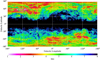 |
Fig. 1 Sky positions of the 7 855 871 profiles with less than eight Gaussians in the central emission peak. The positions of the simplest profiles are marked by the reddest colors. Among the profiles with an equal number of Gaussians those with lower column density of the local H I are plotted with redder color. |
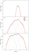 |
Fig. 2 Distribution of the widths of Gaussians for the profiles decomposed to one (upper panel), two (middle panel), or three (lowerpanel) components. |
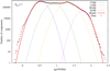 |
Fig. 3 Distribution of the widths of the Gaussians for the profiles with NG ≤ 7. |
2.4 Separating HI phases
So far we have modeled the average frequency distribution of the widths of the Gaussians from profiles with NG ≤ 7 in the velocity range, preselected in Haud & Kalberla (2007), but when plotting the frequency distribution of these Gaussians in the component central velocity – line-width plane (Fig. 4), we can see that at different velocities the distribution of the widths is different. In our trial to separate three H I phases, we decided to take into account also the velocity dependence of the Gaussian widths in different gas phases. For this we assumed that in each narrow velocity range the distribution of the widths of the Gaussians can be modeled with the sum of four log-normal functions, as in Figs. 2 and 3, but the parameters of the log-normal model distributions may change with the velocity.
To estimate the reliability of the obtained models, we decided to construct many different models and to analyze their average results together with corresponding deviations. Altogether six families of the models were constructed, each with many sub-models. All these models were based on the same Gaussian decomposition of the HI4PI H I profiles but differed from each other by the approaches, used for the modeling of the distribution of the Gaussian parameters in their central velocity – line-width plane. For the following we define the model family as a group of models, based on some more or less general assumptions or fitting strategies, related to all models of this group. The sub-models in the family differ then from each other by the usage of different velocity resolutions, profile complexities and initial approximations for the non-linear model fitting. For example, in all families separate models were made for the complexity limits NG ≤ 3, 4, 5, 6, or 7 local Gaussians per observed H I profile. A brief overview of our model families is given in Table 1. The differences between the model families are defined in the second and the third columns of this table and the last column describes the velocity ranges, used in the sub-models of the corresponding family.
In the first two model families, we assumed that the changes in the parameters of the four log-normal distributions with the velocity can be described with the polynomial functions, which contain adjustable parameters. In the first family we used the sixth order polynomial of velocity and in the second family the fourth order polynomial of the function arctan(p5 + p6vc), where p5 and p6 were also adjustable model parameters. For sub-models we analyzed profiles with different complexity NG and their Gaussians from different velocity ranges (as specified in Table 1). We divided all Gaussians in the analyzed velocity ranges into 200 groups, each containing the same number of components with similar velocities. In this way the usage of different velocity ranges gave us also different velocity resolutions of the corresponding models. By adjusting the parameters of the polynomials, describing the velocity dependencies of three parameters in each of four log-normal distribution, we represented the complete distribution of the Gaussians (as in Fig. 4) with some model distribution (one possible example in Fig. 5) by minimizing the RMS deviations between observed and model distributions in all velocity and line-width bins.
To define the initial approximation for all models in these two families, we searched in each velocity bin of Fig. 4 for the line widths, corresponding to the local frequency maxima and recorded their velocities, Gaussian widths and the breadths, Δ, of the lg (FWHM) regions, in which the corresponding point was a global maximum. The results are given as blue points in Fig. 4. The sizes of the points are proportionalto Δ. The found maxima were classified by hand into four groups, corresponding to four log-normal functions, fitting the frequency distribution of the Gaussians. The initial dependencies of the centers of the log-normal functions on the velocity were then defined as fits of the polynomials through the corresponding points of the local maxima in the observed frequency distribution. For this fitting, the values of Δ were used as weights. The results are given in Fig. 4 by magenta lines. Initial approximations of the heights of the log-normal distributions were determined by fitting the family specific polynomials through the Gaussian frequencies at the points calculated from the functions found for the centers of the log-normal distributions.
From the preceding experience on the modeling of the Gaussian frequency distributions in the fixed velocity range (Figs. 2 and 3), it was clear that the most uncertain property of the log-normal distributions is their width. Therefore, the initial approximations for the widths of the log-normal distributions were determined as constants from the velocity range − 3.39 < vc < −1.26 km s−1, where the LNM is most clearly separated from CNM and WNM (Fig. 4). When starting the final model fitting, these constants were used for all velocities (the coefficients of the velocity dependent terms of the corresponding functions were all taken to be equal to zero), but during the fitting of the models the coefficients of all terms were allowed to vary freely.
For the fitting of the models, we used the multidimensional downhill simplex method and for the first two families of the models we generated up to five subfamilies with different algorithms for the generation of the initial simplex. When the model converged to some solution, we generated a new large simplex around the obtained result and repeated the fitting until the repetitions did not yield any considerable improvements in the results. Due to a large number of the free fitting parameters, such repetitions generally found deeper minima than those obtained in the first run of the fitting.
All together we obtained in both model families up to 150 different models. In each obtained model we searched the velocity dependent values of the line widths at which the modeled frequency of the Gaussians in two neighboring (on the order of increasing line widths) gas phases were equal. The obtained values of FWHMCL(vc), FWHMLW(vc), and FWHMWX(vc) for the borders between CNM – LNM, LNM – WNM, and WNM – XNM components were converted into corresponding Doppler temperatures TD,CL(vc), TD,LW(vc), and TD,WX(vc), where
 (2)
(2)
and averaged over all models of one family. The standard deviations of the results from different models were considered as error estimates of the results.
An example of the model from the second family for |vc | < 100 km s−1 and NG ≤ 7 is given in Fig. 5. Here the isolines represent the observed distribution from Fig. 4 and the background colors give the model approximation of these lines. Blue dashed curves give the locations of the peaks of the log-normal model curves (the magenta lines from Fig. 4 after the model fitting) and the solid blue lines are the line widths, which separate different gas phases.
The upper left corner of Fig. 5 demonstrates that at higher velocities the behavior of the models was sometimes so wild that it was impossible to define the separating line widths. At the same time, at low velocities the polynomial models were even more stable than we expected in advance. Therefore, we decided to take a step further and to construct additional model families, in which we dropped the requirement of the polynomial dependence of the parameters of the log-normal distributions on the velocity, but analyzed the width distributions only for |vc | < 50 km s−1. In the last four families of the models we turned back to the fitting of the width distributions in the narrow velocity ranges, as it was described in Sect. 2.3, but for each fit we defined an independent velocity region for the fitting. The velocity ranges were constructed randomly so that they contained at least 19 000 and at most 210 000 Gaussians and all Gaussians had equal probabilities to be included in some velocity range. For each model the upper limit of the profile complexity was also randomly chosen so that NG ≤ 3, 4, 5, 6, or 7.
In each of these four additional families we used a different approach to the fitting of the models and generated 60 000 independentsub-models for different velocity ranges and profile complexities. For all these models the initial approximations were taken from the final models of the second polynomial family. For families three and four we minimized the parameter 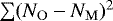 , but for families five and six we used
  , where NO and NM are the numbers of the Gaussians in different width bins from our Gaussian decomposition and from the corresponding model, respectively.In this way the families three and four were mostly sensitive to the ridges of the frequency distributions, but five and six gave more weight to the wings of the distributions. In families three and five we did not apply any additional restrictions to the model fitting, but in families four and six we also demanded that during the fitting process the FWHM, corresponding to the peaks of the model distributions, had to follow the relation FWHMCNM < FWHMLNM < FWHMWNM < FWHMXNM. It was accomplished through the penalty function so that each violation of this rule multiplied the sum of the squares of the residuals by 2.0. Some examples of the models from the last four families are given in Fig. 6.
After constructing the models, the interpretation of the results was similar to that of the polynomial families one and two. We calculated the line widths at which the modeled frequencies of the Gaussians in the neighboring gas phases were equal. The obtained values of the FWHM were converted into the Doppler temperatures, averaged in regular velocity bins over all models of each family and the corresponding standard deviations were calculated as estimates of the result uncertainties.
The comparison of the results indicated that up to about |vc | = 15 km s−1 the different model families were in good mutual agreement. At higher velocities the deviations started to increase (especially at negative velocities for TD,CL – the Doppler temperature, which separates CNM from the LNM), but remained acceptable up to about |vc | = 25 km s−1. At even higher velocities the deviations grow rapidly, which makes the results extremely uncertain. This is rather understandable. We planned to study the local interstellar medium and to test how far our approach may be viable. In Fig. 4 the bands of the CNM and WNM are well visible up to |vc | ≈ 15 km s−1. The blue dots defining the LNM are considerably more scattered, but still the presence of this phase is felt. Beyond |vc | ≈ 15 km s−1 the bands of CNM and WNM turn upward. CNM at negative and WNM at positive velocities becomes also less obvious and the definition of the LNM becomes rather doubtful. At |vc| > 25 km s−1 the identification of the LNM with the intermediate- and high-velocity clouds (the strong frequency enhancements at about lg (FWHM) = 1.35 near the left and right edges of the figure, see Haud 2008) is already more than questionable. These results are also understandable from the comparison of the example models, given in Fig. 6. At low velocities the CNM, LNM, and WNM phases are well defined in the distribution of the Gaussian widths, but at higher velocities their identification becomes more and more doubtful. To avoid possible misidentifications we eventually decided to restrict our analysis to |vc | < 8 km s−1, see Sect. 3.2.
The results for |vc|≤ 25 km s−1 from all model families are summarized in Fig. 7. The values for TD,CL are given in blue, those for TD,LW are in green and red corresponds to TD,WX. The error-bars illustrate the standard deviations of the results in the different model families. The dark thick curves are the polynomial fits (using corresponding standard deviations for computing the weights) to all the presented results and the lighter thick curves illustrate the median uncertainties (for |vc | ≤ 25 km s−1) of the dark curves.
 |
Fig. 4 Frequency distribution of the 42 488 690 Gaussians, used for the modeling of the line-width distributions of the gas phases, in the component central velocity – line-width plane. Blue points mark the local maxima in the frequency distribution of the Gaussian line widths at different velocities and the magenta lines represent initial estimates of the centers of four log-normal model distributions of the Gaussian widths in different gas phases. As abscissa we have used the quantiles of the velocity distribution of the used Gaussians. The numbers mark the values of the deciles. |
Families of the models for the width distributions of the Gaussians at different velocities.
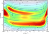 |
Fig. 5 As Fig. 4, but the background colors now correspond to the sub-model for |vc | ≤ 99 km s−1 and NG ≤ 7 from the second model family. The blue dashed lines give the positions of the peaks of the fitted log-normal distributions and solid lines indicate the formal division between the modeled gas phases. |
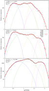 |
Fig. 6 Three examples of the models from the last four families. In the upper panel is the model from the velocity range, where the LNM is most clearly visible in Fig. 4. The middle panel corresponds to the velocities, close to the limit |vc | ≤ 8 km s−1, used for the discussions in the present paper and the lower panel illustrates the situation at extreme velocities |vc | = 25 km s−1, used for Fig. 7. |
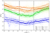 |
Fig. 7 Results for TD,CL (blue), TD,LW (green), and TD,WX (red) from six model families TD1 − TD6. Each family is plotted with different symbols. The error bars correspond to the standard deviations of the sub-modelsin each family. The polynomial fits to the results from all families are plotted with the thick dark linesand the thick lighter lines give the corresponding median uncertainties in the velocity range |vc | ≤ 25 km s−1. Two vertical black lines indicate the velocity range |vc|≤ 8 km s−1, used for the discussions. |
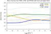 |
Fig. 8 Velocity dependencies for phase fractions fCNM (blue), fLNM (green), and fWNM (orange), plotted with thick lines, and their upper and lower limits (thin). |
3 Derived properties of discrete H I phases
So far, when deriving criteria to distinguish Gaussians belonging to different phases, we used only profiles with simple structures, corresponding to decompositions with NG ≤ 7 components.For a meaningful analysis of the H I distribution on the sky we need to generalize our results and assume that the derived criteria do not depend significantly on the number of clouds along the line of sight or the complexity of the profiles, represented by NG.
We sort Gaussian components according to their center velocities and Doppler temperatures, using the velocity dependent thresholds from Fig. 7, and group the components for separate phases. These different groups of Gaussians are then used to generate individual synthetic profiles TbP for the phases P = CNM, LNM, and WNM with a velocity grid of δvLSR = 1 km s−1 on an nside = 1024 HEALPix grid in position. Thus we replace the observed H I distribution by three separate distributions to model the CNM, LNM, and WNM. As mentioned earlier, the WNM includes the contributions from the XNM. The sum of these phase dependent distributions fits to the observed brightness distribution Tb; we only omit Gaussians representing obvious instrumental problems (Kalberla & Haud 2015). When generating maps we smooth these brightness temperatures to an effective beam-size of 30′ FWHM.
To measure, how much of the H I gas belongs to a particular phase we define phase fractions 
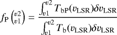 (3)
(3)
for P = CNM, LNM, and WNM.
Phase fractions are in general velocity dependent but for simplicity we drop this notation in the following. We will see later that phase fractions depend significantly on environmental effects.
3.1 Velocity dependencies
Velocity dependencies of derived single channel phase fractions are shown in Fig. 8. We display a comparison of the average all-sky phase fractions for − 8 < vLSR < 8 km s−1 (thick lines) for the individual phases. Velocity dependencies are obvious, in particular fCNM and fWNM show systematic fluctuations.
Figure 8 includes also estimates for the uncertainties of the derived average phase fractions (thin lines). For all of the phases we used median standard deviations for the thresholds between the linewidth regimes (see Fig. 7) to derive upper and lower limits for the phase fractions. The uncertainties are significant, up to 50%, in particular for the LNM since this phase is affected by uncertainties in the thresholds for both, the CNM and the WNM phase.
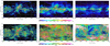 |
Fig. 9 Top panel: All-sky plate carrée (CAR) display of the observed H I brightness temperature distributions at a velocity of vLSR = 0 km s−1, distinguishing contributions from the CNM (left), LNM (middle), and WNM (right). The color scale is linear from TB = 0 K to TB = 40 K. Bottom panel: H I phase fractions fCNM (left), fLNM (middle), and fWNM (right) for the same data. Galactic coordinates are used, the Galactic Center is in the middle. |
3.2 All-sky maps for CNM, LNM, and WNM
In this section we show all-sky distributions of separate phases to give a first impression of morphological differences between the different phases. We use a plate carrée projection1.
In Fig. 9 we use a single velocity channel at vLSR = 0 km s−1 to show the separate components. At the top we display the brightness temperature contributions for CNM (left), LNM (middle), and WNM (right). At the bottom we show with the same sequence the corresponding phase fractions fCNM, fLNM, and fWNM according to Eq. (3).
These all-sky maps display a surprising wealth of large and small scale structures. For the CNM and the LNM there are dominant filamentary features but even the fWNM map shows remarkable structures, either with high or low fWNM fractions. The WNM maps are barely compatible with a diffuse medium, the usual description we find in textbooks. In fact, in case of ongoing thermal instabilities we expect some anti-correlations between CNM on one hand and LNM or WNM on the other side. Such anti-correlations will be discussed in Sects. 4 and 6.
Figure 10 gives an alternative representation of the all-sky column density distribution for the velocity range − 8< vLSR < 8 km s−1. With the same sequence of the phases as in Fig. 9 we display at the top lg (NH∕[cm−2]). At the bottom we show the corresponding phase fractions. Interestingly, phase fractions in Figs. 9 and 10 (bottom) show in general very similar structures. This result can be explained by the velocity distribution of dominant local H I structures (Kalberla et al. 2016; Sect. 5.13) that can be fit well with a Gaussian of FWHM of 16.8 km s−1, centered at vLSR = 0 km s−1. The local H I gas is dominated by low velocity structures in this range.
The top panels of Figs. 9 and 10 for the WNM (right hand side) show enhancements of the H I emission in the Galacticplane with a sin(2l) modulation. A similar but less obvious effect is visible for the LNM (middle panels). These enhancements are caused by differential Galactic rotation (Mebold 1972) and imply for the Galactic plane that some of the observed gas must originate from large distances. At these positions our basic assumption, that we consider only local H I gas, is violated. Surprisingly, when calculating phase fractions (lower panels of Figs. 9 and 10) these contamination are less obvious. Apparently the contaminations cancel mostly when calculating phase fractions. Anyhow, our caveat is that phase fractions at low Galactic latitudes are in general less reliable, this includes also larger uncertainties from the Gaussian analysis at low latitudes.
The separation of individual H I phases in Sect. 2.4 leads to significant velocity dependencies of the TD thresholds, as shown in Fig. 7. These velocity dependencies are relatively weak for the velocity range − 8< vLSR < 8 km s−1 but increase significantly at higher velocities. Since this velocity range covers most of the local H I gas features, as presented inFigs. 9 and 10, we decided to restrict our analysis to this velocity range.
3.3 Average column density distributions
The column density distributions for different phases can be derived in two ways. Either by selecting Gaussian components according to the velocity dependent thresholds derived in Sect. 2.4 and generating then maps for a FWHM beam-size of 30′. This results in the spatial distributions displayed in Figs. 9 and 10. Alternatively we may derive the column density distributions directly from the Gaussian database, using appropriate phases and center velocities. Figure 11 shows the results for the velocity range − 8 < vLSR < 8 km s−1. We display data for the CNM, LNM, and WNM (left to right) restricted to latitudes |b| > 20° but also for all-sky.
Figure 11 shows in all cases column density distributions that are close to log-normal, the best fit Gaussians are included for comparison. For the CNM we plot also the distributions for filamentary structures derived from unsharp masked (USM) maps (Kalberla et al. 2016; their Fig. 12). Such features emphasize the H I distribution at high spatial frequencies. This gas is cold and aligned with polarized dust emission (Clark et al. 2014; Kalberla et al. 2016). The USM structures have low column densities and represent only a subset of the CNM emission. These features have barely direct counterparts in the list of Gaussian components. In the right hand panel of Fig. 11 we show also the H I distribution for the XNM, the fourth phase from Figs. 2 to 7 that we consider as part of the WNM.
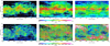 |
Fig. 10 Top panel: All-sky display of the observed H I column density distributions, integrating over a velocity range − 8 < vLSR < 8 km s−1 and distinguishing contributions from the CNM (left), LNM (middle), and WNM (right). The color scale is logarithmic, lg (NH ∕[cm−2]). Bottom panel: H I phase fractions fCNM (left), fLNM (middle), and fWNM (right) for the same data. Galactic coordinates are used, the Galactic Center is in the middle. |
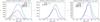 |
Fig. 11 Distribution functions for column densities lg(NH∕[cm−2]) of the CNM (left), LNM (middle), and WNM (right), derived from Gaussian components in the velocity range − 8 < vLSR < 8 km s−1. The light and dark blue colors distinguishes distributions for all Sky and |b| > 20°. The green lines show in each case least square Gaussian fits, resulting in log-normal distributions. For the CNM (left panel) we include the distributions of major filamentary USM structures as observed by Kalberla et al. (2016; their Fig. 12). On the right hand side the XNM components are also included for comparison. |
3.4 Column densities depending on phase fractions
Here we derive dependencies between column densities and phase fractions according to Eq. (3). We use the velocity range − 8 < vLSR < 8 km s−1. Figure 12 displays separately for each of the gas phases 2D density distributions for column densities and phase fractions. On the top the data are restricted to high latitudes |b| > 20°, below we plot all-sky data.
High latitude data show the cleanest relations between column densities and phase fractions. The all-sky distributions are more complex due to some additional structures originating from regions close to the Galactic plane. However, in both cases the LNM standsout with a distribution that differs significantly from the CNM and the WNM. The LNM exists mostly with phase fractions 0.3≲fLNM≲0.6.
Figure 12 shows a clear dependency between column density distributions of individual H I phases and the corresponding phase fractions. This may imply that phases with distinct different temperatures are separated from each other. Figures 9 and 10 show in fact some evidence for regions that are dominated by one or the other phase.
3.5 Average phase fractions
For the velocity range − 8 < vLSR < 8 km s−1 we determine all-sky average phase fractions 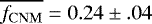 ,
,  , and
, and 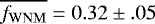 . Here the listed uncertainties come only from the velocity dependent fluctuations of phase fractions for − 8< vLSR < 8 km s−1. Systematic errors may be much larger, see Sect. 2.4 and Fig. 8. Restricting our sample to high Galactic latitudes |b| > 20° we obtain
 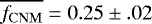 ,
,  , and
, and  . As detailed in Sect. 3.2 we consider the derived parameters close to the Galactic plane as uncertain. Still the all-sky results agree within the errors with average phase fractions from high latitudes.
 |
Fig. 12 2D density distribution functions in the velocity range − 8 < vLSR < 8 km s−1 for CNM (left), LNM (middle), and WNM (right), showing the relations between phase fractions and column densities lg (NH ∕[cm−2]) for each phase. Top panel: positions with |b| > 20°, bottom panel: all sky data. |
4 CNM and WNM dominated regions
A comparison between Figs. 9 and 10 shows that the all-sky distribution of the CNM phase is most prominent at velocities close to zero. We use therefore the range − 1< vLSR < 1 km s−1 to separate CNM dominated regions from the rest of the H I distribution by applying a mask. To define CNM dominated regions we first select only positions with fCNM > 0.5. This map of delta functions, representing cold spots, is smoothed by a Gaussian function with FWHM = 5°; the resulting map is truncated at 10% of the peak. Values above this threshold are set to one and values below to zero respectively. Approximately 22% of the total sky is this way masked as CNM dominated.
The application of this mask allows a separation of CNM dominated regions including a homogeneous area around the most prominent CNM structures. Figure 13 shows in the upper panel CNM dominated areas separated from the rest of the sky. The CNM structures are surrounded by LNM but there is little WNM associated with the CNM. Some borders of the CNM dominated regions appear to have enhanced WNM as a transition to the regions displayed on the lower panels of Fig. 13 that have been masked out from the CNM dominated areas. Our masking procedure is subjective, we have tried to work out an environment around the CNM with a smooth boundary at the transition between cold (CNM dominated) and warm (WNM dominated) H I regions.
4.1 Average phase fractions in CNM and WNM dominated regions
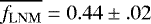
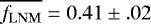
Calculating average phase fractions for |b| > 20° and − 8< vLSR < 8 km s−1 we come for CNM dominated regions to the striking result that these regions are actually not dominated by the CNM but by LNM:  ,
,  , and
, and 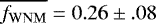 . The situation is similar for the rest of the sky, the WNM dominated part:
 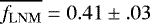 ,
, 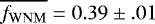 , and
, and 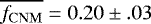 . Thus, we obtain the unexpected result that in both cases the LNM is dominant. The average LNM phase fraction
  , determined in Sect. 3.5, appears to be characteristic for most of the sky if we consider the velocity range − 8< vLSR < 8 km s−1.
4.2 Phase fractions around cold spots
To define the CNM dominated regions shown in Fig. 13 on top we selected a smoothing kernel K with a FWHM of 5^°. For a more general analysis, proposed by the referee, we extend here our calculations for the range 0.5° ≤ K ≤ 10°. In addition we use several velocity ranges for the determination of average phase fractions.
The topleft panel of Fig. 14 shows a generalization of the results from the previous subsection.  decreases for increasing K. At the same time we find an increase of
  . This implies that the CNM is on average localized; as we increase the area around the cold spots we observe on average less CNM but more LNM.
  and
and  are anti-correlated; the LNM surrounds the cold spots. In addition we find that also
  is gradually increasing with K. The response of the WNM is much smoother than that of the LNM, implying than the WNM is distributed on average over large scales. This confirms essentially the visual impression we get from the right hand side of Fig. 13.
The middle and right hand side panels on top of Fig. 14 show even clearer correlations between CNM, LNM, and WNM for restricted velocity windows − 4 ≤ vLSR ≤ 4 km s−1 and − 1 ≤ vLSR ≤ 1 km s−1.  increases with decreasing velocity width but
  remains almost unaffected. The implication is that the CNM in cold spots is not only spatially localized but also restricted in velocity space. The LNM is spatially extended, surrounding the CNM, and covers in addition a larger velocity spread. The WNM has a line-width of typically 24 km s−1,
  contributes correspondingly less with decreasing velocity width. This effect apparently tends to balance the LNM phase fraction, we observe
  for different choices of the averaging line-width. In the lower panels of Fig. 14 we present our results for an all-sky analysis, confirming essentially the conclusions from high latitudes.
4.3 Dust temperatures associated with HI phases
The all-sky maps displayed in Figs. 9, 10, and 13 show for the CNM some common structures with filamentary H I gas and the Planck HFI Sky Map at 353 GHz (see Kalberla et al. 2016; their Fig. 2); the CNM is associated with polarized dust emission. To find out whether our masking for cold and warm H I gas results also in regions with physically distinct different dust temperatures we intend to correlate now the H I distribution with the dust temperature distribution.
Currently the most reliable dust temperatures are available from Planck Collaboration Int. XLVIII (2016). These authors used a tailored component-separation method, the so-called generalized needlet internal linear combination (GNILC) method, which uses spatial information (angular power spectra) to disentangle the Galactic dust emission and anisotropies in the cosmic infrared background.
To determine phase dependent relations between H I column densities and dust temperatures we use Gaussian components with center velocities in the range − 8 < vLSR < 8 km s−1 at latitudes |b| > 20°. Corresponding to the cases selected in Fig. 13 (CNM top and WNM bottom) we plot in Fig. 15 phase dependent 2D density distribution functions for dust temperatures and column densities for different H I phases.
The average dust temperature determined by Planck Collaboration Int. XLVIII (2016) is Tdust = 19.41 ± 1.54 K. All H I phases in the CNM dominated part of the sky (Fig. 15 top) are characterized by low dust temperatures. H I column densities are high, in particular for the CNM and LNM. For the rest of the sky (bottom) we find warmer dust with temperatures around 19.4 K for the CNM and WNM, but for the LNM even some of the H I gas reaches dust temperatures close to 20 K.
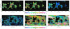 |
Fig. 13 All-sky distribution functions for phase fractions in the velocity range − 1 < vLSR < 1 km s−1. Left panel: CNM, middle panel: LNM, and right panel: WNM. We distinguish CNM dominated regions, shown on top, and WNM dominated regions at bottom. |
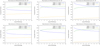 |
Fig. 14 Phase fractions for CNM dominated regions depending on the width of the smoothing kernel used for the generation of the mask. Top panel: high latitudes |b| > 20° only, bottom panel: all sky data. From left to right: phase fractions for |vLSR| < 8, |vLSR | < 4, and |vLSR| < 1 km s−1 are shown. |
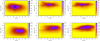 |
Fig. 15 2D density distribution functions showing the relations between dust temperatures and column densities for Gaussiancomponents in the velocity range − 8 < vLSR < 8 km s−1 at latitudes |b| > 20°. Components from CNM dominated regions are shown on top, the remaining sample at bottom. Left to right: CNM, LNM, and WNM components. |
4.4 Phase dominated positions for f > 2/3
Next we consider the question how far dust temperatures depend on H I phase fractions. As before, we consider CNM and WNM dominated regions on the sky (Fig. 13). We select there positions where each of the H I phases is dominant. To decide whether a phase is predominant we use the condition f∕(1 − f) > C. Thus we demand that the amount of H I in an individual phase has to be a factor of C > 1 larger than the sum of the remaining phase fractions for the other phases. Figure 16 shows the distribution of dust temperatures derived for the case C = 2 or f > 2∕3. This factor is somewhat arbitrary (though widely used to define a qualified majority) but our results do not depend significantly on C. For all C > 1 we get well defined dust temperature distributions that can be approximated by Gaussians. To the left of Fig. 16 we plotted the selected cold CNM dominated part, to the right the warm WNM dominated sky and in the middle the unconstrained sample. Each of the distributions is fitted by a Gaussian to obtain mean dust temperatures with dispersions that are listed in Table 2.
These histograms show for all phases that the CNM dominated part of the local H I distribution is cold with typical dust temperatures Tdust ~ 18.7 K. There is little WNM with fWNM≳2∕3. Opposite, the WNM dominated regions have Tdust ~ 19.4 K and there is only little CNM. The unconstrained H I distribution is dominated by the LNM with intermediate temperatures, Tdust ~ 19 K. The upper plots in Fig. 16 are for high Galactic latitudes, |b| > 20°, the lower plots display the all-sky distribution. The reliability of the all-sky histograms is somewhat questionable but we include these to demonstrate that they share the same trend as the histograms for high latitudes.
Our results are consistent with the average Tdust = 19.41 ± 1.54 K as determined by Planck Collaboration Int. XLVIII (2016) at high latitudes. However, Fig. 16 indicates a general dependency that dust temperatures decrease in regions that are dominated by the CNM. Each of the dust components can be fitted by Gaussians (see Table 2). For the CNM dominated sample the fits are well defined with low dispersions around one K. The distributions for the WNM dominated sky are broader and may contain several components with some scatter. Thelower panel in Fig. 16 indicates that also some more scatter may exist at latitudes |b|≲20°.
Figure 16 confirms the trends from Fig. 15 but we need to point out that in particular positions with fCNM≳2∕3 that are associated with cold dust are almost exclusively found in the CNM dominated part of the sky. Opposite, positions with fWNM≳2∕3 and warm dust are less frequent in this areas. For the rest of the sky we observe a dominance of the WNM, but surprisingly also there the LNM is significant. In all cases, for f≳2∕3, we find low-dust temperatures for CNM dominated regions and opposite high temperatures in case of the WNM dominated sky, see Table 2. Thus, the dust temperatures are more smoothly distributed compared to the H I gas that may have significant local fluctuations in phase fractions.
Dust temperatures associated with CNM, LNM, and WNM at phase fractions f > 2∕3.
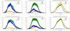 |
Fig. 16 Frequency distribution for dust temperatures in selected regions on the sky. From left to right: CNM dominated, unconstrained, and WNM dominated according to Fig. 13. Top panel: data at |b| > 20° in the velocity range − 8 < vLSR < 8 km s−1 are used for fCNM > 2∕3 (blue), fLNM > 2∕3 (green), and fWNM > 2∕3 (yellow). Bottom panel: the same distribution for all-sky. |
5 Cold and filamentary H I
A significant fraction of the cold H I gas exists in filamentary structures that can be worked out for high resolution H I observations by unsharp masking (Kalberla et al. 2016). Many of these filaments are associated with dust and the most prominent filaments are aligned with the magnetic field. In this section we want to explore temperature dependencies of the different phases in presence of such filamentary structures.
Using the USM data from Kalberla et al. (2016), we search at each position for the strongest filament in the velocity range − 8 < vLSR < 8 km s−1 and calculate its Doppler temperature TD. We demand an USM peak temperature of at least one K. If such a feature is found we determine the velocity channel corresponding to its center velocity v0. We use one additional channel on both sides and determine for this velocity window of 3 km s−1 the phase fractions fCNM, fLNM, and fWNM. Our analysis is restricted to filamentary H I structures at high latitudes |b| > 20°. Figure 17 displays on top the derived 2D density distributions for Doppler temperatures and phase fractions f.
Next weconsider the question how the observed dust temperatures might depend on H I phase fractions for filamentary H I. For a comparison between dust temperatures and H I Doppler temperatures we determine at each position with a known USM Doppler temperature TD the corresponding GNILC dusttemperature Tdust. In Fig. 17 we present on bottom 2D density distributions for dust temperatures associated with filamentary H I structures. Comparing Doppler temperatures at top of Fig. 17 with dust temperatures at bottom we find similar trends for different phase fractions; fCNM, fLNM, and fWNM (left to right).
These plots show that Doppler and dust temperatures in filaments decrease on average with increasing CNM fraction fCNM. The vertical stripe at fCNM ~ 0 in the left panels of Fig. 17 indicates that some of the USM filaments are not identified with proper Gaussian components. For an approximate threshold fCNM≲0.05 we find that less than 4% of the USM filaments are affected. For the other data we fit lg (TD∕[K]) = 2.5222 ± 0.0008 − (0.451 ± 0.002) ⋅ fCNM for the H I and Tdust = 19.455 ± 0.002 − (0.643 ± 0.004) ⋅ fCNM K for the dust. The median Doppler temperatureis TD = 203 K, corresponding to a median dust temperature of Tdust = 19.08 K.
The median temperature for dust associated with filamentary H I is colder than the average temperature of Tdust = 19.41 ± 1.54 K (Planck Collaboration Int. XLVIII 2016). The H I filaments selected in the current analysis are also slightly colder than the filaments studied in Kalberla et al. (2016) with a median Doppler temperature of TD = 223 K. Prominent cold filaments reach fCNM ~ 0.65 (see Fig. 18, also Appendix B). Typical Doppler temperatures are 170 K, with dust temperatures of 19 K. Such Doppler temperatures correspond to a FWHM line width of 3.2 km s−1 and our sliding velocity window with δvLSR = 3 km s−1 matches well with this line width. We conclude that the ISM in local filamentary structures is comparatively cold.
The middle and lower plots in Fig. 17 show that the Doppler and dust temperatures in filaments are also correlated with the component fraction fLNM and fWNM of the associated warmer gas. For the LNM we fit for the H I lg(TD∕[K]) = 2.1789 ± 0.0008 + (0.3600 ± 0.002) ⋅ fLNM; for the dust Tdust = 19.165 ± 0.002 − (0.012 ± 0.004) ⋅ fLNM K. For the WNM we obtain lg(TD∕[K]) = 2.24195 ± 0.0005 + (0.50156 ± 0.003) ⋅ fWNM and Tdust = 18.994 ± 0.002 + (1.070 ± 0.006) ⋅ fWNM K.
This implies that the Doppler temperatures of USM filaments tend to increase moderately up to typical temperatures around TD = 228 K and Tdust = 19.17 K for an LNM environment with a component fraction of fLNM = 0.5. Such a H I Doppler temperature differs only slightly from the median of TD = 223 K determined by Kalberla et al. (2016). For filaments embedded in WNM with fLNM = 0.5 we obtain a significantly higher Doppler temperature TD = 311 K and correspondingly a higher dust temperature Tdust = 19.53 K. The temperature differences would increase further for larger WNM component fractions, however we observe little filaments associated with WNM in this state (Fig. 17 bottom). This deficiency may imply that we observe here a transition to ionized gas.
Calculating average phase fractions for filaments we find that such regions are dominated by the CNM: fCNM ~ 0.46, fLNM ~ 0.37, and fWNM ~ 0.17. Here fCNM is a lower limit only, our data are not corrected for optical depth effects, for discussion see Kalberla et al. (2016; Sect. 5.9). Optical depth effects however are mostly negligible for lg(NH∕[cm−2])≲20.6 (Lee et al. 2015). Figures 12 and 15 show that most of the CNM at high latitudes is below this limit.
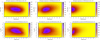 |
Fig. 17 H I in filaments. 2D density distribution functions for phase fractions and USM Doppler temperatures TD (top) as well as associated dust temperatures Tdust (bottom) in filaments at |b| > 20°; left: CNM, middle: LNM, and right: WNM phase fractions. |
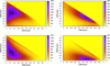 |
Fig. 18 All sky 2D distribution functions, showing how frequent phase fractions of different phases are related to each other for |b| > 20° in the velocity range − 8 < vLSR < 8 km s−1. Top for CNM and LNM and bottom for CNM and WNM. Left panel: unconstrained H I data; right panel: filamentary H I structures only. |
6 H I phases along the line of sight
The results from the previous sections imply that the different H I phases are associated with each other; the observed gas composition changes according to the environment. In Sect. 4.2, considering the extension of CNM dominated regions in the plane of the sky, we demonstrated that there is an anti-correlation between  and
and  .
.
To study further the relationship between CNM, LNM, and WNM we determine the 2D frequency distributions of the observed phase fractions at the same position, hence along the line of sight. We use latitudes |b| > 20° and the velocity range − 8 < vLSR < 8 km s−1. Figure 18 shows how frequent the CNM with a phase fraction fCNM is associated with LNM or WNM and phase fractions fLNM or fWNM respectively.To the left we display unconstrained data. In this case the CNM contributes typically little H I gas with fCNM≲0.15. The distribution is bimodal. The associated warmer gas belongs either to the LNM with typically fLNM ~ 0.55 or to the WNM with fWNM ~ 0.3. Thus the LNM is dominant, in agreement with Fig. 16.
The filamentary H I gas has a very different composition. This is demonstrated on the right hand side of Fig. 18. In this case only filamentary H I structures from the USM database have been selected. Clearly, filaments are outstanding with high phase fractions fCNM. Further a sharp division between the associated LNM and WNM phases is visible. The LNM typically occupies regions with larger phase fractions fLNM compared to the WNM. The sharp diagonal stripe in the upper panel on the right hand side of Fig. 18 confirms that also in filamentary H I structures CNM and LNM are closely anti-correlated. The anti-correlation between CNM and WNM, shown in the panel below, has a larger scatter.
7 Discussion
Our most important result is the large average phase fraction  and the close anti-correlation between LNM and CNM. Most obvious are the phase relations from the distribution of the different phases around cold spots (Sect. 4.2). The detailed anti-correlation between
  and
and  on small and intermediate scales proves that the clumpy CNM is embedded in LNM. The WNM surrounds both phases with an anti-correlation on larger scales. The same kind of layered structure is observed around cold filaments. These filaments are associated with cold dust. Doppler temperatures as well as dust temperatures decrease with increasing fCNM.
When distinguishing H I associated with cold filamentary structures as described in Sect. 5 from the unconstrained H I distribution it needs to be considered that filamentary structures most probably are caused by sheets, seen edge-on (Heiles & Troland 2005; Kalberla et al. 2016, 2017). Similar structures with different orientations, such that we do not have a favorable tangential view (amplifying projected column densities), may exist but these parts of the H I distribution will not be observable with an outstanding morphology. On the other hand, also H I clouds that are warmer than the filaments may contribute to the diffuse H I phase.
From H I observations alone it is difficult to decide whether the WNM shown in Fig. 18 on the right hand side is physically related to the CNM but we see in Fig. 17 that a significant part of WNM in filaments is associated with particular cold dust that appears to be more smoothly distributed than the H I. So we are apparently left with a miracle; warm H I gas associated with cold dust along the line of sight. This phenomenon may be explainable in context with the McKee & Ostriker (1977) model. The prediction is that cold gas must be associated with warmer gas, in addition there should even be some ionized material at the same velocity. Indeed, Kalberla et al. (2017) demonstrated that radio-polarimetric filaments can be associated with cold H I filaments. H I Doppler temperatures were found to be correlated with the CNM phase fractions and a re-inspection of the Auriga and Horologium fields considered by Kalberla et al. (2017) discloses that some of the USM filaments are also associated with cold dust filaments.
Phase fractions discussed by Kalberla et al. (2017) were based on the simplified assumption of a two-phase H I medium. Nevertheless, it was shown that increasing CNM phase fractions are correlated with decreasing H I Doppler temperatures and at the same time with anisotropies. In addition steep spectral indices were found for the associated turbulence power spectra that appear to be related to phase transitions. For a bi-modal H I distribution such a steepening is hardly explainable. Considering local instabilities within a smoothly distributed WNM phase we expect in case of phase transitions a cold gas distribution with enhanced structures on small scales. This implies a local flattening of the power spectrum, contrary to observations.
Our investigations prove that the CNM is associated with significant amounts of LNM. The CNM is clumpy, the anti-correlation between fCNM and fLNM implies therefore that the LNM must be surrounding the colder gas on larger scales, up to scales of a few degrees. For an average phase fraction  this results necessarily in excess LNM emission around the CNM. Thus, the presence of LNM on larger scales leads to enhancedemission on such scales, offering a natural explanation for the observed steepening of local power spectra.
The Gaussian decomposition resulted in the following mean FWHM line-widths of the CNM, LNM, and WNM gas: 3.6, 9.6, and 23.3 km s−1, corresponding to Doppler temperatures of 283, 2014, and 11 870 K. These results can be used to estimate characteristic turbulent Mach numbers for the H I phases;  (Heiles & Troland 2003a). Using a typical kinetic temperature of 50 K for the CNM (Heiles & Troland 2003a) we obtain MCNM = 4.4. USM filaments have somewhat lower Doppler temperatures and correspondingly 3.2≲MCNM≲3.7 (Kalberla et al. 2016). For the LNM it is hardly possible to define a characteristic kinetic temperature. Using a lower limit of 500 K we derive a firm upper limit MLNM≲3.6 for the LNM Mach number. In case of the WNM we derive MWNM ~ 1.4 for an kinetic temperature of 8000 K. There is a systematic trend that Mach numbers decrease with increasing Doppler temperatures for the different phases.
Our result that filamentary H I gas is associated with cold dust might be explainable by destruction of dust. Anisotropies in the observed H I distribution are probably caused by cold shells or sheets, seen edge-on. As suggested by Heiles & Troland (2003a), these structures result from shock waves, originating from supernova explosions, causing phase transitions and rapid cooling of the H I. Such shocks can destroy also grains through sputtering. Large grains are ground down into smaller grains (Jones et al. 1996). Low CNM temperatures in filaments may thus be explainable by reduced photoelectric heating due to depletion of polycyclic aromatic hydrocarbons (PAHs; Wolfire et al. 2003) but a direct observational evidence for such a process is difficult for the dust (Tielens 2008). Micelotta et al. (2010) model PAH processing in interstellar shocks and find that PAHs do not survive shocks with velocities greater than 100 km s−1. We like to point out that we observe low dust temperatures only for cold filamentary H I gas. Without Doppler temperatures from USM data we would not be able to quantify a relation between dust and Doppler temperatures. The main evidence for such a correlation comes from our USM data in direction to Loop I (Egger & Aschenbach 1995). This is a prominent object and Loop I at an age of several 106 yr is still expanding at a velocity of 17.3 km s−1 (Frisch & Dwarkadas 2018). A depletion of PAHs appears plausible under these conditions.
Dust variations in the diffuse interstellar medium have also been noted by Ysard et al. (2015). These authors use total H I column densities from the LAB survey at high Galactic latitudes for 1019 ≲NH≲2.5 × 1020 cm−2 with a sky coverage of about 12%. They show that variations in the dust properties observed with Planck-HFI cannot be explained by variations in the radiation field intensity and gas density distribution. They conclude that small variations in the dust properties can explain most of the variations in the dust emission observed by Planck-HFI in the diffuse ISM. Unfortunately, due to their column density limit, this analysis excludes Loop I and most of the regions with cold H I filaments.
One of the main drivers for the launch of Plank was the quest to observe the cosmic microwave background B-mode signal induced by primordial gravitational waves during cosmic inflation. However, there are Galactic foregrounds and it is now established that these are a main limiting factor for accurate cosmological parameters. Polarized Galactic foreground observations with Planck and H I emission data indicate that most of the filamentary dust structures are embedded in filamentary CNM structures (Clark et al. 2014; Kalberla et al. 2016). Based on this finding Ghosh et al. (2017) constructed a phenomenological dust model, combining H I data with an astrophysically motivated description of the large-scale and turbulent Galactic magnetic field. They modeled the large-scale polarized dust emission over the southern Galactic cap by using GASS H I data with selected velocity dispersions. They were able to reproduce the Planck dust observations at 353 GHz for a region of 3500 deg2 at the southern Galactic cap. They tested their model for H I velocity dispersions σ < 3 km s−1 and 3 < σ < 7.5 km s−1 and found no significant differences. These two ranges correspond approximately to our CNM and LNM linewidth regimes. Thus the results by Ghosh et al. (2017) are consistent with our conclusion that cold CNM filaments and the surrounding LNM must be related to each other.
8 Summary and conclusion
We used a Gaussian decomposition of the HI4PI survey to separate and model the CNM, LNM, and WNM distributions. Our main resultsare as follows:
Phase fractions depend on the selected velocity range. For the velocity range − 8< vLSR < 8 km s−1 41% of the local H I gas is LNM. Next important is the WNM with 34%, the CNM contributes only 25%. CNM or LNM are never observed as a single phases, they can only coexist with WNM. The phase fractions for CNM and LNM are anti-correlated. This impliesthat the LNM surrounds the clumpy CNM. Both phases are embedded in the smoothly distributed WNM.
CNM dominated regions have low dust temperatures, Tdust ~ 18.5 K. The dust in WNM dominated regions is warmer; differences amount to about 1 K. Dust temperatures as well as Doppler temperatures for CNM in filaments decrease with increasing fCNM. Outside H I filaments dust temperatures show a general trend to increase with LNM and WNM column densities. Here the presence of CNM (typically with fCNM≲0.2) does not correlate with dust temperatures.
The previous conclusions are based on high latitudes |b| > 20°. An extrapolation to lower latitudes suffers from large uncertainties but closer to the Galactic plane we did not get significantly different results. It is difficult to define clear criteria for the separation of CNM, LNM, and WNM. The derived H I phase fractions may be uncertain by 50%. Such uncertainties do however not invalidate our general conclusions.
Previous studies have shown that cold filamentary H I structures in the diffuse interstellar medium are associated with dust ridges, aligned with the magnetic field measured on the structures by Planck at 353 GHz (Clark et al. 2014; Kalberla et al. 2016). These are also the structures where we find high values for fCNM and low dust temperatures. It is becoming increasingly evident that the state of the ISM is significantly affected by feedback processes.
Acknowledgements
We thank the referee, Carl Heiles, for constructive criticism that helped to improve the paper, also Jürgen Kerp for valuable discussions and continuous support. U.H. acknowledges the support by the Estonian Research Council grant IUT26-2, and by the European Regional Development Fund (TK133). This research has made use of NASA’s Astrophysics Data System. EBHIS is based on observations with the 100-m telescope of the MPIfR (Max-Planck-Institut für Radioastronomie) at Effelsberg. The Parkes Radio Telescope is part of the Australia Telescope which is funded by the Commonwealth of Australia for operation as a National Facility managed by CSIRO. Some of the results in this paper have been derived using the HEALPix package.
Note added in proof. After acceptance of the manuscript the 21-SPONGE H I absorption line survey against 57 background continuum sources became available (Murray et al. 2018). These authors distinguish H I phases for derived spin temperatures with Ts < 250 K for the CNM, 250 < Ts < 1000 K for the unstable LNM, and Ts > 1000 K for the WNM. Accordingly they conclude that 28% of the H I mass is associated with the CNM, 20% belongs to the LNM, and 52% to the WNM. We determine for the region covered by this survey mostly dust temperatures between 19 and 19.5 K, independent of preferences in phase fractions, and  ,
,  , and
, and  . Murray et al. (2018) do not detect a significant mass fraction for H I at 1000≲Ts≲4000 K. The LNM is a transient phase. We explain discrepancies in the derived LNM and WNM phase fractions as an indication
that only about half of the LNM observed by us is currently evolving to cold structures with recognizable optical depths.
Appendix A On the XNM
In this paper we discuss CNM, LNM, and WNM phases of H I, but Figs. 2, 3, and 6 contain also the fourth curve – XNM. We mentioned that in many cases, but not always, the XNM Gaussians seem to be caused by the wide but weak wings of the lines from other phases. In a Gaussian decomposition such lines cannot be described by a single component as the Gaussians fall off too rapidly compared to the data. However, such lines are often successfully modeled with the Voigt profile(Mitchell & Zemansky 1971) – a convolution of a Gaussian function with a Lorentzian, or, due to the computational expense of the convolution operation, the Voigt profile is approximated with a pseudo-Voigt one. Here we try to give a brief test, if such a more complicated fitting procedure may help us to avoid the XNM components in our decomposition.
From the middle panel of Fig. 2, we can see that the XNM is well visible already for profiles, decomposed with only two low-velocity Gaussians. With such profiles it is easy to estimate the presumable improvements in the results, obtainable by using of Voigt profiles. However, the Voigt profiles are only able to describe symmetric non-Gaussian wings. Therefore, it is important to estimate, how symmetric is the XNM component in each profile located relative to another Gaussian of the same H I profile.
To study the symmetry of the simple profiles, we selected from our Gaussian database 51 726 profiles with NG = 2, in which at least one Gaussian had the width, typical for XNM (lg(FWHM) > 1.64 from Fig. 2). For each profile we computed the positive velocity difference Δ vc between thecenters of the two Gaussians. Figure A.1 gives the distribution of the contributions (the percentage from the total column density of the XNM, represented by the selected profiles), of the XNM components with different shifts relative the main components of the profiles. We can see that the maximum of the distribution corresponds to a considerable shift between the centers of the Gaussians. However, due to the observational noise we cannot expect that the centers of the Gaussians, which describe the main H I peak and its wide wings coincide exactly and the acceptable mismatch increases with the increasing width of the XNM component.
We have studied the influence of the observational noise to the uncertainties of the Gaussian parameters in Haud (2000) and on the basis of this study we expect that for our selected XNM Gaussians with average FWHM = 56.5 km s−1, the shifts up to about Δvc = 6 km s−1 (broad green line in Fig. A.1) between the centers of two components in each profile may yet be acceptable for fitting both of these Gaussians with the symmetric Voigt profile. From Fig. A.1 we can see that most (about 79%) of the XNM column density in studied simple profiles comes from the Gaussians with larger displacements relative to the main component. Corresponding profiles must be clearly asymmetric and for these we cannot expect good fits with symmetric Voigt profiles. Moreover, the Gaussians, which represent base-line problems or other asymmetric features, may be centered anywhere on the velocity axis, but the wings, describable by the Voigt profiles must be centered near our present main component of the corresponding profile. Therefore, even at Δ vc < 6 km s−1 we may expect some contribution from features for which modeling with the Voigt profiles may be questionable and therefore 100 − 79 = 21% is an upper limit for the fraction of simple profiles that can be modeled successfully with Voigt profiles.
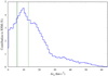 |
Fig. A.1 Fractions of the total column density of the XNM from profiles with NG = 2 as a functionof the velocity difference Δvc between thecenters of their Gaussian components. The shifts up to the thick green line are likely explainable with the uncertainties in the Gaussian decomposition and the thin green line marks the median of the distribution. |
Of course, the estimate for the permissible displacement of the Gaussians for successful fitting with the Voigt profile, is relatively uncertain and it may be possible that contrary to our expectations even
at higher displacements satisfactory fits with Voigt profiles exist. To test this, we give two examples in Fig. A.2. The upper panel corresponds to nearly ideal case for fitting with the Voigt profile with Δ vc= 0.06 km s−1. The reduced χ2 values for fits with Gaussian components and with the pseudo-Voigt profile are  and
and  , respectively.Both these values satisfy our requirements for a good fit (see Sect. 2.2) and as the fit with the pseudo-Voigt profile contains less free parameters we would prefer this model. Such a choice removes from the decomposition of this profile the XNM component and replaces the line width of the WNM Gaussian FWHMG = 23.6 km s−1 with slightly higher value FWHMV = 24.3 km s−1, but this change is considerably smaller than other uncertainties in the separation of different gas phases.
 |
Fig. A.2 Two example fits of the observations with the Gaussian components and with the pseudo-Voigt profile. The upper panel corresponds to the nearly ideal case for the fitting with the pseudo-Voigt profile and the lower panel represents the typical situation. Thick lines correspond to the observations and the models. Thin lines illustrate the Gaussian and the Lorentzian contributions to the final models. Crosses mark the points, which define FWHMWMS in two different models. |
For the lower panel of Fig. A.2 we have chosen a more typical example. Δ vc= 10.14 km s−1 is close to the maximum of the distribution in Fig. A.1, but still less than the median of that distribution at Δ vc= 13.2 km s−1 (thinner green line in Fig. A.1). The contribution of the XNM component to the column density of this profile (NXNM∕NTot = 0.39) is also close to the median (NXNM∕NTot = 0.40) of the corresponding distribution. As we can see, this profile is fitted well with Gaussians ( ), but the fit with the pseudo-Voigt profile is not any more a satisfactory replacement for the XNM component (
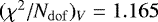 ). The change of the line width is also considerably larger (from FWHMG = 25.8 km s−1 to FWHMV = 28.1 km s−1), but as for a final fit we need at least one more pseudo-Voigt profile, the interpretation of the changes becomes already complicated.
Indirect indication that the modeling of the H I profiles with more general line shapes, other than Gaussians, cannot solve the problems with the XNM, can be seen also from Fig. A.3, which gives the distribution of the XNM fraction, fXNM, in the sky. Except the galactic plane, the fXNM is often the highest in the sky areas, where the total column density is low (see Fig. 2. in HI4PI Collaboration 2016). This is in particular true for the prominent region 130 < l < 190circ and 50 < b < 70circ. There are extended regions with brightness temperatures Tb < 0.5 K at vLSR ~ 0 km s−1 and for such a low emission remaining instrumental problems (RFI, baseline problems and residual stray radiation errors) can easily trigger Gaussian components that are interpreted as XNM. Problems of this kind are recognizable as boxy structures, discontinuities at the borders of individual observing sessions in RA/DEC. About 0.5% of all positions are affected. Demanding for a better reliability of XNM components a more stringent limit of Tb ≳1 K, we find that 3% of the XNM Gaussians may possibly be affected by instrumental problems. The XNM fraction is high also in the first and fourth quadrants near the galactic plane, where the column density of the H I is the highest, but there the different features in the line profiles are so heavily blended with each other that any decomposition of these profiles becomes unreliable, yielding many components with very different properties. About 6% of all positions are affected. In our study we have avoided making conclusions on the basis of the observations near the galactic plane and have used corresponding Gaussians only for tests of the limits, to which the results, obtained from higher latitudes, are applicable.
 |
Fig. A.3 All-sky distribution of the fractions fXNM, integrated over a velocity range − 8 < vLSR < 8 km s−1. |
Therefore, there are certainly cases, where the usage of the Voigt profiles may give better results for the profile decomposition, but we cannot expect that they will solve most of the problems with XNM. Using Voigt profiles for the real symmetric wings of the H I lines improves (increases) somewhat our line-width estimates, but by fitting asymmetric lines or some combinations of the real lines with more questionable features may introduce additional uncertainties to the line-width estimates and as we cannot in all cases automatically distinguish the line wings and the more problematic features, the real gain from the more complicated mathematics may remain rather questionable. As a result, we consider the usage of the Voigt profiles in the present work impractical.
We conclude that a Gaussian decomposition appears to provide a reasonable parametrization of the XNM. About 3% of the XNM may be explainable as instrumental, additional 6% in the Galactic plane as affected by confusion. The rest appears to be associated with WNM structures, mostly asymmetric. This is of course not a proof that such structures must be real. The problem is more general, the question is how to treat extended profile wings when processing instrumental baselines of H I survey observations. Extended asymmetric profile wings may easily be fitted away as baseline errors but the approaches for the LAB (Kalberla et al. 2005), GASS (Kalberla & Haud 2015), and EBHIS (Winkel et al. 2016a) were conservative, taking care that such wings are not eliminated.
Appendix B Total column density distributions with uncertainties
With Fig. 12 we presented 2D distributions for column densities associated with individual phases. A more concise presentationis possible if we summarize the column densities for all gas at a particular phase fraction. For an optical thin medium, assuming further that the distances of the three different observed gas phases do on average not vary significantly, the total column density is proportional to the total mass of the gas associated with a particular phase fraction.
Figure B.1 shows for each of the phases how phase fraction and contributing column densities are related to each other. We distinguish between H I associated with cold USM filaments (top) and H I observed outside such filamentary structures (bottom). As detailed in Sect. 2.4, the separation of the CNM, LNM, and WNM is burdened with rather large uncertainties (see also Fig. 8). To get an impression how far such uncertainties affect the derived distributions, we compare several cases; the best fit result (middle) together with distributions that were derived after applying thresholds offset by the median standard deviation when separating the individual gas phases. We distinguish two characteristic cases, resulting in an upper limit for the CNM and WNM, implying a lower limit for the LNM (max CNM, max WNM, and min LNM, Fig. B.1 left) and a lower limit for the CNM and WNM, implying an upper limit for the LNM (min CNM, min WNM, and max LNM respectively, Fig. B.1 right).
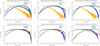 |
Fig. B.1 Normalized column density distribution functions for the phase fractions of the CNM, LNM, and WNM phases at high latitudes |b| > 20°. Top panel: USM filaments in the velocity range − 8 < vLSR < 8 km s−1. Bottom panel: H I outside filaments at constant velocities − 1 < vLSR < 1 km s−1. Middle panel: best fit results according to Fig. 8, Sect. 3.1. Left: minimum LNM, implying maximum CNM and WNM phase fractions. Right: maximum LNM with minimum CNM and WNM fractions respectively. |
The upper panels of Fig. B.1 show that CNM is dominant in USM filaments with large phase fractions. A large amount of the gas is concentrated in cold condensations, fCNM ~ 0.65. Most of the CNM is associated with LNM, correspondingly with fLNM ~ 0.4. The WNM is unimportant with fWNM ~ 0.15. H I gas thatis not associated with filaments (bottom) is characterized by a broad range of observed phase fractions for all phases, in particular for the CNM. The LNM tends to have predominantly fLNM≳0.5 while fWNM≲0.5.
Comparing the upper panels of Fig. B.1 with the lower ones, confirms our previous finding that filamentary H I is special in the sense that the filamentary CNM is dominant for these structures. Correspondingly the total CNM fraction is in this case twice as high as for the non-filamentary sample. Filamentary H I contains little WNM, only half of the fraction derived for the non-filamentary sample, see Fig. 18 for a complementary view.
The comparison plots (left and right hand side of Fig. B.1) show how far the variation of the thresholds with phase contributions that we annotate as min or max affect the derived CNM, LNM, and WNM distributions. In general the column density distributions are shifted to higher phase fractions for the max cases and opposite to lower for the min cases. However the observed variations do not invalidate the conclusions drawn above that filamentary H I structures are enhancements in CNM, associated predominantly with LNM envelopes that have significant phase fractions fLNM. The WNM envelopes are in total less important.
References
- Audit, E., & Hennebelle, P. 2005, A&A, 433, 1 [NASA ADS] [CrossRef] [EDP Sciences] [Google Scholar]
- Clark, S. E., Peek, J. E. G., & Putman, M. E. 2014, ApJ, 789, 82 [NASA ADS] [CrossRef] [Google Scholar]
- de Avillez, M. A., & Breitschwerdt, D. 2005, A&A, 436, 585 [NASA ADS] [CrossRef] [EDP Sciences] [Google Scholar]
- Dickey, J. M., & Lockman, F. J. 1990, ARA&A, 28, 215 [NASA ADS] [CrossRef] [MathSciNet] [Google Scholar]
- Dickey, J. M., Salpeter, E. E., & Terzian, Y. 1977, ApJ, 211, L77 [NASA ADS] [CrossRef] [Google Scholar]
- Dickey, J. M., McClure-Griffiths, N. M., Gaensler, B. M., & Green, A. J. 2003, ApJ, 585, 801 [NASA ADS] [CrossRef] [Google Scholar]
- Egger, R. J., & Aschenbach, B. 1995, A&A, 294, L25 [NASA ADS] [Google Scholar]
- Field, G. B., Goldsmith, D. W., & Habing, H. J. 1969, ApJ, 155, L149 [NASA ADS] [CrossRef] [Google Scholar]
- Fitzpatrick, E. L., & Spitzer, L., Jr. 1997, ApJ, 475, 623 [NASA ADS] [CrossRef] [Google Scholar]
- Frisch, P., & Dwarkadas, V. V. 2018 [arXiv:1801.06223] [Google Scholar]
- Gazol, A., Vázquez-Semadeni, E., Sánchez-Salcedo, F. J., & Scalo, J. 2001, ApJ, 557, L121 [NASA ADS] [CrossRef] [Google Scholar]
- Ghosh, T., Boulanger, F., Martin, P. G., et al. 2017, A&A, 601, A71 [NASA ADS] [CrossRef] [EDP Sciences] [Google Scholar]
- Górski, K. M., Hivon, E., Banday, A. J., et al. 2005, ApJ, 622, 759 [NASA ADS] [CrossRef] [Google Scholar]
- Haud, U. 2000, A&A, 364, 83 [NASA ADS] [Google Scholar]
- Haud, U. 2008, A&A, 483, 461 [NASA ADS] [CrossRef] [EDP Sciences] [Google Scholar]
- Haud, U., & Kalberla, P. M. W. 2007, A&A, 466, 555 [NASA ADS] [CrossRef] [EDP Sciences] [Google Scholar]
- Heiles, C. 2001, ApJ, 551, L105 [NASA ADS] [CrossRef] [Google Scholar]
- Heiles, C., & Troland, T. H. 2003a, ApJ, 586, 1067 [NASA ADS] [CrossRef] [Google Scholar]
- Heiles, C., & Troland, T. H. 2003b, ApJS, 145, 329 [NASA ADS] [CrossRef] [Google Scholar]
- Heiles, C., & Troland, T. H. 2005, ApJ, 624, 773 [NASA ADS] [CrossRef] [Google Scholar]
- Hennebelle, P., & Falgarone, E. 2012, A&ARv, 20, 55 [NASA ADS] [CrossRef] [Google Scholar]
- HI4PI Collaboration, (Ben Bekhti, N., et al.) 2016, A&A, 594, A116 [NASA ADS] [CrossRef] [EDP Sciences] [Google Scholar]
- Jones, A. P., Tielens, A. G. G. M., & Hollenbach, D. J. 1996, ApJ, 469, 740 [NASA ADS] [CrossRef] [Google Scholar]
- Kalberla, P. M. W., & Haud, U. 2015, A&A, 578, A78 [NASA ADS] [CrossRef] [EDP Sciences] [Google Scholar]
- Kalberla, P. M. W., Schwarz, U. J., & Goss, W. M. 1985, A&A, 144, 27 [NASA ADS] [Google Scholar]
- Kalberla, P. M. W., Burton, W. B., Hartmann, D., et al. 2005, A&A, 440, 775 [NASA ADS] [CrossRef] [EDP Sciences] [Google Scholar]
- Kalberla, P. M. W., McClure-Griffiths, N. M., Pisano, D. J., et al. 2010, A&A, 521, A17 [NASA ADS] [CrossRef] [EDP Sciences] [Google Scholar]
- Kalberla, P. M. W., Kerp, J., Haud, U., et al. 2016, ApJ, 821, 117 [NASA ADS] [CrossRef] [Google Scholar]
- Kalberla, P. M. W., Kerp, J., Haud, U., & Haverkorn, M. 2017, A&A, 607, A15 [NASA ADS] [CrossRef] [EDP Sciences] [Google Scholar]
- Lee, M.-Y., Stanimirović, S., Murray, C. E., Heiles, C., & Miller, J. 2015, ApJ, 809, 56 [NASA ADS] [CrossRef] [Google Scholar]
- McClure-Griffiths, N. M., Pisano, D. J., Calabretta, M. R., et al. 2009, ApJS, 181, 398 [NASA ADS] [CrossRef] [Google Scholar]
- McKee, C. F.,& Ostriker, J. P. 1977, ApJ, 218, 148 [NASA ADS] [CrossRef] [Google Scholar]
- Mebold, U. 1972, A&A, 19, 13 [NASA ADS] [Google Scholar]
- Mebold, U., Winnberg, A., Kalberla, P. M. W., & Goss, W. M. 1982, A&A, 115, 223 [NASA ADS] [Google Scholar]
- Micelotta, E. R., Jones, A. P., & Tielens, A. G. G. M. 2010, A&A, 510, A36 [NASA ADS] [CrossRef] [EDP Sciences] [Google Scholar]
- Mitchell, A. G. G., & Zemansky, M. W. 1971, Resonance radiation and excited atoms (Cambridge: Cambridge University Press) [Google Scholar]
- Mohan, R., Dwarakanath, K. S., & Srinivasan, G. 2004, JA&A, 25, 143 [NASA ADS] [CrossRef] [Google Scholar]
- Murray, C. E., Stanimirović, S., Goss, W. M., et al. 2015, ApJ, 804, 89 [NASA ADS] [CrossRef] [Google Scholar]
- Murray, C. E., Stanimirović, S., Kim, C.-G., et al. 2017, ApJ, 837, 55 [NASA ADS] [CrossRef] [Google Scholar]
- Murray, C. E., Stanimirovic, S., Goss, W. M., et al. 2018, ApJS, 238, 14 [NASA ADS] [CrossRef] [Google Scholar]
- Nidever, D. L., Majewski, S. R., & Butler Burton, W. 2008, ApJ, 679, 432 [NASA ADS] [CrossRef] [Google Scholar]
- Planck Collaboration Int. XLVIII. 2016, A&A, 596, A109 [NASA ADS] [CrossRef] [EDP Sciences] [Google Scholar]
- Roy, N., Kanekar, N., & Chengalur, J. N. 2013, MNRAS, 436, 2366 [NASA ADS] [CrossRef] [Google Scholar]
- Salpeter, E. E. 1976, ApJ, 206, 673 [NASA ADS] [CrossRef] [Google Scholar]
- Saury, E., Miville-Deschênes, M.-A., Hennebelle, P., Audit, E., & Schmidt, W. 2014, A&A, 567, A16 [NASA ADS] [CrossRef] [EDP Sciences] [Google Scholar]
- Spitzer, L., Jr.& Fitzpatrick, E. L. 1995, ApJ, 445, 196 [NASA ADS] [CrossRef] [Google Scholar]
- Takakubo, K., & van Woerden, H. 1966, Bull. Astron. Inst. Netherlands, 18, 488 [Google Scholar]
- Tielens, A. G. G. M. 2008, ARA&A, 46, 289 [NASA ADS] [CrossRef] [EDP Sciences] [Google Scholar]
- Vázquez-Semadeni, E. 2012, EAS Pub. Ser., 56, 39 [Google Scholar]
- Winkel, B., Kerp, J., Flöer, L., et al. 2016a, A&A, 585, A41 [NASA ADS] [CrossRef] [EDP Sciences] [Google Scholar]
- Winkel, B., Lenz, D., & Flöer, L. 2016b, A&A, 591, A12 [NASA ADS] [CrossRef] [EDP Sciences] [Google Scholar]
- Wolfire, M. G., Hollenbach, D., McKee, C. F., Tielens, A. G. G. M., & Bakes, E. L. O. 1995, ApJ, 443, 152 [Google Scholar]
- Wolfire, M. G., McKee, C. F., Hollenbach, D., & Tielens, A. G. G. M. 2003, ApJ, 587, 278 [NASA ADS] [CrossRef] [Google Scholar]
- Ysard, N., Köhler, M., Jones, A., et al. 2015, A&A, 577, A110 [NASA ADS] [CrossRef] [EDP Sciences] [Google Scholar]
On request HEALPix nside = 1024 FITS files that can be used to generate other projections are available from the first author.
All Tables
Families of the models for the width distributions of the Gaussians at different velocities.
All Figures
|
Fig. 1 Sky positions of the 7 855 871 profiles with less than eight Gaussians in the central emission peak. The positions of the simplest profiles are marked by the reddest colors. Among the profiles with an equal number of Gaussians those with lower column density of the local H I are plotted with redder color. |
| In the text | |
|
Fig. 2 Distribution of the widths of Gaussians for the profiles decomposed to one (upper panel), two (middle panel), or three (lowerpanel) components. |
| In the text | |
|
Fig. 3 Distribution of the widths of the Gaussians for the profiles with NG ≤ 7. |
| In the text | |
|
Fig. 4 Frequency distribution of the 42 488 690 Gaussians, used for the modeling of the line-width distributions of the gas phases, in the component central velocity – line-width plane. Blue points mark the local maxima in the frequency distribution of the Gaussian line widths at different velocities and the magenta lines represent initial estimates of the centers of four log-normal model distributions of the Gaussian widths in different gas phases. As abscissa we have used the quantiles of the velocity distribution of the used Gaussians. The numbers mark the values of the deciles. |
| In the text | |
|
Fig. 5 As Fig. 4, but the background colors now correspond to the sub-model for |vc | ≤ 99 km s−1 and NG ≤ 7 from the second model family. The blue dashed lines give the positions of the peaks of the fitted log-normal distributions and solid lines indicate the formal division between the modeled gas phases. |
| In the text | |
|
Fig. 6 Three examples of the models from the last four families. In the upper panel is the model from the velocity range, where the LNM is most clearly visible in Fig. 4. The middle panel corresponds to the velocities, close to the limit |vc | ≤ 8 km s−1, used for the discussions in the present paper and the lower panel illustrates the situation at extreme velocities |vc | = 25 km s−1, used for Fig. 7. |
| In the text | |
|
Fig. 7 Results for TD,CL (blue), TD,LW (green), and TD,WX (red) from six model families TD1 − TD6. Each family is plotted with different symbols. The error bars correspond to the standard deviations of the sub-modelsin each family. The polynomial fits to the results from all families are plotted with the thick dark linesand the thick lighter lines give the corresponding median uncertainties in the velocity range |vc | ≤ 25 km s−1. Two vertical black lines indicate the velocity range |vc|≤ 8 km s−1, used for the discussions. |
| In the text | |
|
Fig. 8 Velocity dependencies for phase fractions fCNM (blue), fLNM (green), and fWNM (orange), plotted with thick lines, and their upper and lower limits (thin). |
| In the text | |
|
Fig. 9 Top panel: All-sky plate carrée (CAR) display of the observed H I brightness temperature distributions at a velocity of vLSR = 0 km s−1, distinguishing contributions from the CNM (left), LNM (middle), and WNM (right). The color scale is linear from TB = 0 K to TB = 40 K. Bottom panel: H I phase fractions fCNM (left), fLNM (middle), and fWNM (right) for the same data. Galactic coordinates are used, the Galactic Center is in the middle. |
| In the text | |
|
Fig. 10 Top panel: All-sky display of the observed H I column density distributions, integrating over a velocity range − 8 < vLSR < 8 km s−1 and distinguishing contributions from the CNM (left), LNM (middle), and WNM (right). The color scale is logarithmic, lg (NH ∕[cm−2]). Bottom panel: H I phase fractions fCNM (left), fLNM (middle), and fWNM (right) for the same data. Galactic coordinates are used, the Galactic Center is in the middle. |
| In the text | |
|
Fig. 11 Distribution functions for column densities lg(NH∕[cm−2]) of the CNM (left), LNM (middle), and WNM (right), derived from Gaussian components in the velocity range − 8 < vLSR < 8 km s−1. The light and dark blue colors distinguishes distributions for all Sky and |b| > 20°. The green lines show in each case least square Gaussian fits, resulting in log-normal distributions. For the CNM (left panel) we include the distributions of major filamentary USM structures as observed by Kalberla et al. (2016; their Fig. 12). On the right hand side the XNM components are also included for comparison. |
| In the text | |
|
Fig. 12 2D density distribution functions in the velocity range − 8 < vLSR < 8 km s−1 for CNM (left), LNM (middle), and WNM (right), showing the relations between phase fractions and column densities lg (NH ∕[cm−2]) for each phase. Top panel: positions with |b| > 20°, bottom panel: all sky data. |
| In the text | |
|
Fig. 13 All-sky distribution functions for phase fractions in the velocity range − 1 < vLSR < 1 km s−1. Left panel: CNM, middle panel: LNM, and right panel: WNM. We distinguish CNM dominated regions, shown on top, and WNM dominated regions at bottom. |
| In the text | |
|
Fig. 14 Phase fractions for CNM dominated regions depending on the width of the smoothing kernel used for the generation of the mask. Top panel: high latitudes |b| > 20° only, bottom panel: all sky data. From left to right: phase fractions for |vLSR| < 8, |vLSR | < 4, and |vLSR| < 1 km s−1 are shown. |
| In the text | |
|
Fig. 15 2D density distribution functions showing the relations between dust temperatures and column densities for Gaussiancomponents in the velocity range − 8 < vLSR < 8 km s−1 at latitudes |b| > 20°. Components from CNM dominated regions are shown on top, the remaining sample at bottom. Left to right: CNM, LNM, and WNM components. |
| In the text | |
|
Fig. 16 Frequency distribution for dust temperatures in selected regions on the sky. From left to right: CNM dominated, unconstrained, and WNM dominated according to Fig. 13. Top panel: data at |b| > 20° in the velocity range − 8 < vLSR < 8 km s−1 are used for fCNM > 2∕3 (blue), fLNM > 2∕3 (green), and fWNM > 2∕3 (yellow). Bottom panel: the same distribution for all-sky. |
| In the text | |
|
Fig. 17 H I in filaments. 2D density distribution functions for phase fractions and USM Doppler temperatures TD (top) as well as associated dust temperatures Tdust (bottom) in filaments at |b| > 20°; left: CNM, middle: LNM, and right: WNM phase fractions. |
| In the text | |
|
Fig. 18 All sky 2D distribution functions, showing how frequent phase fractions of different phases are related to each other for |b| > 20° in the velocity range − 8 < vLSR < 8 km s−1. Top for CNM and LNM and bottom for CNM and WNM. Left panel: unconstrained H I data; right panel: filamentary H I structures only. |
| In the text | |
|
Fig. A.1 Fractions of the total column density of the XNM from profiles with NG = 2 as a functionof the velocity difference Δvc between thecenters of their Gaussian components. The shifts up to the thick green line are likely explainable with the uncertainties in the Gaussian decomposition and the thin green line marks the median of the distribution. |
| In the text | |
|
Fig. A.2 Two example fits of the observations with the Gaussian components and with the pseudo-Voigt profile. The upper panel corresponds to the nearly ideal case for the fitting with the pseudo-Voigt profile and the lower panel represents the typical situation. Thick lines correspond to the observations and the models. Thin lines illustrate the Gaussian and the Lorentzian contributions to the final models. Crosses mark the points, which define FWHMWMS in two different models. |
| In the text | |
|
Fig. A.3 All-sky distribution of the fractions fXNM, integrated over a velocity range − 8 < vLSR < 8 km s−1. |
| In the text | |
|
Fig. B.1 Normalized column density distribution functions for the phase fractions of the CNM, LNM, and WNM phases at high latitudes |b| > 20°. Top panel: USM filaments in the velocity range − 8 < vLSR < 8 km s−1. Bottom panel: H I outside filaments at constant velocities − 1 < vLSR < 1 km s−1. Middle panel: best fit results according to Fig. 8, Sect. 3.1. Left: minimum LNM, implying maximum CNM and WNM phase fractions. Right: maximum LNM with minimum CNM and WNM fractions respectively. |
| In the text | |
Current usage metrics show cumulative count of Article Views (full-text article views including HTML views, PDF and ePub downloads, according to the available data) and Abstracts Views on Vision4Press platform.
Data correspond to usage on the plateform after 2015. The current usage metrics is available 48-96 hours after online publication and is updated daily on week days.
Initial download of the metrics may take a while.