| Issue |
A&A
Volume 619, November 2018
|
|
|---|---|---|
| Article Number | A27 | |
| Number of page(s) | 20 | |
| Section | Extragalactic astronomy | |
| DOI | https://doi.org/10.1051/0004-6361/201833136 | |
| Published online | 07 November 2018 | |
The MUSE Hubble Ultra Deep Field Survey
XI. Constraining the low-mass end of the stellar mass – star formation rate relation at z < 1⋆
1
Leiden Observatory, Leiden University, PO Box 9513
2300 RA, Leiden, The Netherlands
e-mail: This email address is being protected from spambots. You need JavaScript enabled to view it.
2
Instituto de Astrofísica e Ciências do Espaço, Universidade do Porto, CAUP, Rua das Estrelas, PT4150-762
Porto, Portugal
3
IRAP (Institut de Recherche en Astrophysique et Planétologie), Université de Toulouse, CNRS, UPS, Toulouse, France
4
CRAL, Observatoire de Lyon, CNRS, Université Lyon 1, 9 Avenue Ch. André, 69561 Saint Genis Laval Cedex, France
5
Department of Physics, ETH Zürich, Wolfgang–Pauli–Strasse 27, 8093
Zürich, Switzerland
6
Leibniz-Institut für Astrophysik Potsdam (AIP), An der Sternwarte 16, 14482 Potsdam, Germany
7
Harvard-Smithsonian Center for Astrophysics, 60 Garden St., 02138 Cambridge, MA, UK
Received:
30
March
2018
Accepted:
20
July
2018
Abstract
Star-forming galaxies have been found to follow a relatively tight relation between stellar mass (M*) and star formation rate (SFR), dubbed the “star formation sequence”. A turnover in the sequence has been observed, where galaxies with M* < 1010 M⊙ follow a steeper relation than their higher mass counterparts, suggesting that the low-mass slope is (nearly) linear. In this paper, we characterise the properties of the low-mass end of the star formation sequence between 7 ≤ log M*[M⊙] ≤ 10.5 at redshift 0.11 < z < 0.91. We use the deepest MUSE observations of the Hubble Ultra Deep Field and the Hubble Deep Field South to construct a sample of 179 star-forming galaxies with high signal-to-noise emission lines. Dust-corrected SFRs are determined from Hβ λ4861 and Hα λ6563. We model the star formation sequence with a Gaussian distribution around a hyperplane between logM*, logSFR, and log(1 + z), to simultaneously constrain the slope, redshift evolution, and intrinsic scatter. We find a sub-linear slope for the low-mass regime where log SFR [M⊙yr−1] = 0.83+0.07−0.06 log M*[M⊙]+1.74+0.66−0.68 log(1 + z), increasing with redshift. We recover an intrinsic scatter in the relation of σintr = 0.44+0.05−0.04, dex, larger than typically found at higher masses. As both hydrodynamical simulations and (semi-)analytical models typically favour a steeper slope in the low-mass regime, our results provide new constraints on the feedback processes which operate preferentially in low-mass halos.
Key words: galaxies: star formation / galaxies: formation / galaxies: evolution / galaxies: ISM / methods: statistical
Based on observations made with ESO telescopes at the La Silla Paranal Observatory under programme IDs ID 060.A-9100(C), 094.A-2089(B), 095.A-0010(A), 096.A-0045(A), and 096.A-0045(B).
© ESO 2018
1. Introduction
How galaxies grow is one of the fundamental questions in astronomy. The picture that has emerged is that a galaxy builds up its stellar mass mainly through star formation, which is triggered by gas accretion from the cosmic web (e.g. Dekel et al. 2009; Van de Voort et al. 2012), while mergers with other galaxies play only a minor role (except for massive systems; Bundy et al. 2009).
In the past decade, star-forming galaxies have been found to form a reasonably tight quasi-linear relation between stellar mass (M*) and star formation rate (SFR; Brinchmann et al. 2004; Noeske et al. 2007b; Elbaz et al. 2007; Daddi et al. 2007; Salim et al. 2007) over a wide range of masses and out to high redshifts (Pannella et al. 2009; Santini et al. 2009; Santini et al. 2017; Oliver et al. 2010; Peng et al. 2010; Rodighiero et al. 2010; Karim et al. 2011; Bouwens et al. 2012; Whitaker et al. 2012, 2014; Stark et al. 2013; Ilbert et al. 2015; Lee et al. 2015; Renzini & Peng 2015; Schreiber et al. 2015; Shivaei et al. 2015; Salmon et al. 2015; Tasca et al. 2015; Gavazzi et al. 2015; Kurczynski et al. 2016; Tomczak et al. 2016; Bisigello et al. 2018), which is often referred to as the “main sequence of star-forming galaxies” or the “star formation sequence”. In contrast, galaxies that are undergoing a starburst or have already quenched their star formation lie respectively above and below the relation. This main sequence is close to a similar scaling relation for halos (Birnboim et al. 2007; Neistein & Dekel 2008; Genel et al. 2008; Fakhouri & Ma 2008; Correa et al. 2015a, b) where the growth rate increases super-linearly1 with halo mass, and this has been interpreted as supporting the picture where galaxy growth is driven by gas accretion from the cosmic web (e.g. Bouché et al. 2010; Lilly et al. 2013; Rodríguez-Puebla et al. 2016; Tacchella et al. 2016).
This interpretation is supported by hydrodynamical simulations of galaxy formation (Schaye et al. 2010; Haas et al. 2013a; Haas et al. 2013b; Torrey et al. 2014; Hopkins et al. 2014; Crain et al. 2015; Hopkins et al. 2016), where a global equilibrium relation is found between the inflow and outflow of gas and star formation in galaxies. In this picture the star formation acts as a self-regulating process, where the inflow of gas, through cooling and accretion, is balanced by the feedback from massive stars and black holes (e.g. Schaye et al. 2010). Furthermore, semi-analytical models (e.g. Dutton et al. 2010; Mitchell et al. 2014; Cattaneo et al. 2011, 2017) and relatively simple analytic theoretical models which connect the gas supply (from the cosmological accretion) to the gas consumption can also reproduce the main features of the main sequence rather well (e.g. Bouché et al. 2010; Davé et al. 2012; Lilly et al. 2013; Dekel et al. 2013; Dekel & Mandelker 2014; Mitra et al. 2015; Rodríguez-Puebla et al. 2016, 2017)2.
The parameters of the M*-SFR relation (i.e. slope, normalisation, and scatter) are thus important, as they provide us with insight into the relative contributions of different processes operating at different mass scales, in particular when comparing the values of the parameters to their counterparts in dark matter halo scaling relations. The normalisation of the star formation sequence is governed by the change in cosmological gas accretion rates and gas depletion timescales. The slope can be sensitive to the effect of various feedback processes acting on the accreted gas, which prevent (or enhance) star formation. The intrinsic scatter around the equilibrium relation is predominantly determined by the stochasticity in the gas accretion process (e.g. Forbes et al. 2014; Mitra et al. 2017), but can also be driven by dynamical processes that rearrange the gas inside galaxies (Tacchella et al. 2016). The M*-SFR relation is observed to be reasonably tight, with an intrinsic scatter of only ≈0.3 dex (Noeske et al. 2007b; Salmi et al. 2012; Whitaker et al. 2012; Guo et al. 2013; Speagle et al. 2014; Schreiber et al. 2015; Kurczynski et al. 2016, though we caution against a blind comparison as different observables probe star formation on different timescales). Yet, it has proven to be challenging to place firm constraints on the intrinsic scatter as one needs to deconvolve the scatter due to measurement uncertainty (e.g. Speagle et al. 2014; Kurczynski et al. 2016; Santini et al. 2017).
Observationally, the slope has been difficult to measure, particularly at the low-mass end, as most studies have been sensitive to galaxies with stellar masses above log M*[M⊙] ∼ 10 and often lack dynamical range in mass. In addition, while it is well known that there is significant evolution in the normalisation of the sequence with redshift, most studies have measured the slope in bins of redshift. For a flux limited sample this could introduce a bias in the slope because overlapping populations at different normalisations are not sampled equally in mass within a single redshift bin. The slope may also be mass dependent and indeed recent studies have observed that the relation turns over around a mass of M* ∼ 1010 M⊙ (Whitaker et al. 2012, 2014; Lee et al. 2015; Schreiber et al. 2015; Tomczak et al. 2016) and shows a steeper slope below the turnover mass. In the low-mass regime, a (nearly) linear slope has generally been expected (e.g. Schreiber et al. 2015; Tomczak et al. 2016), motivated also by the fact that there is very little evolution in the faint-end slope of the blue stellar mass function with redshift (Peng et al. 2014). Leja et al. (2015) showed that the sequence cannot have a slope a < 0.9 at all masses because this would lead to a too high number density between 10 < log M*[M⊙] < 11 at z = 1.
In addition to the observational challenges, careful modelling is required to get reliable constraints on the parameters (slope, normalisation, scatter) of the star formation sequence. It is important to properly take selection effects into account as well as the uncertainties on both the stellar masses and star formation rates (and, if spectroscopy is lacking, also on the photometric redshifts). The latter in particular, due to the fact that there is intrinsic scatter in the relation that needs to be deconvolved from the measurement errors. Common statistical techniques do not take these complications into account self-consistently, which leads to biases in the results.
Putting the existing observations in perspective, it is clear that a large dynamical range in mass is necessary to measure the slope of the star formation sequence in the low-mass regime. Deep field studies, that can blindly detect large numbers of galaxies down to masses much below 1010 M⊙, are invaluable in this regard (e.g. Kurczynski et al. 2016). Yet, such studies are challenged by having to measure all observables, distances as well as stellar masses and star formation rates, from the same photometry. This can lead to undesirable correlations between different observables. At the same time the measurements suffer from the uncertainties associated with photometric redshifts. Spectroscopic follow up is crucial in this regard, but can suffer from biases due to photometric preselection.
With the advent of the Multi Unit Spectroscopic Explorer (MUSE; Bacon et al. 2010) on the VLT it is now possible to address these concerns. With the deep MUSE data obtained over the Hubble Ultra Deep Field (HUDF; Bacon et al. 2017) and Hubble Deep Field South (HUDF; Bacon et al. 2015), we can “blindly” detect star-forming galaxies in emission lines down to very low levels ( ) and obtain a precise spectroscopic redshift estimate at the same time (Inami et al. 2017). These data provides a unique view into the low-mass regime of the star formation sequence.
In this paper we present a characterisation of the low-mass end of the M*-SFR relation, using deep MUSE observations of the HUDF and HDFS. We characterise the properties of the M*-SFR relation down stellar masses of M* ∼ 108 M⊙ and SFR  , out to z < 1, and trace the SFR in individual galaxies with masses as low as M* ≲ 107 M⊙ at z ∼ 0.2. We model the relation using a self-consistent Bayesian framework and describe it with a Gaussian distribution around a plane in (log mass, log SFR, log redshift)-space. This allows us to simultaneously constrain the slope and evolution of the star formation sequence as well as the amount of intrinsic scatter, while taking into account heteroscedastic errors (i.e. a different uncertainty for each data point).
The structure of the paper is as follows. In Sect. 2 we first introduce the MUSE data set and outline the selection criteria used to construct our sample of star-forming galaxies. We then go into the methods used to determine a robust stellar mass and a SFR from the observed emission lines. Before looking at the results, we discuss the consistency of our SFRs in Sect. 3. We then introduce the framework of our Bayesian analysis used to characterise the M*-SFR relation (Sect. 4) and present the results in Sect. 5. We discuss the robustness of the derived parameters in Sect. A.1. Finally, we discuss our results in the context of the literature and models, and the physical implications (Sect. 6). We summarise with our conclusions in Sect. 7. Throughout this paper we assume a Chabrier (2003) stellar initial mass function and a flat ΛCDM cosmology with H0 = 70 km s−1 Mpc−1, Ωm = 0.3 and ΩΛ = 0.7.
2. Observations and methods
To study the properties of the galaxy population down to low masses and star formation rates, deep spectroscopic observations are required for a large number of sources. We exploit the unique observations taken with the MUSE instrument over the Hubble Ultra Deep Field (Bacon et al. 2017) and the Hubble Deep Field South (Bacon et al. 2015) to investigate the star formation rates in low-mass galaxies at 0.11 < z < 0.91. We provide a brief presentation of the observations and data reduction in the next section, but refer to the corresponding papers for details.
The MUSE instrument is an integral-field spectrograph situated at UT4 of the Very Large Telescope. It has a field-of-view of 1′ × 1′ when operating in wide-field-mode, which is fed into 24 different integral-field units. These sample the field-of-view at 0.2′′ resolution. The spectrograph covers the spectrum across 4650 Å–9300 Å with a spectral resolution of R ≡ λ/Δλ ≃ 3000. The result of a MUSE observation is a data cube of the observed field, with two spatial and one spectral axes, i.e. an image with spectroscopic information at every pixel.
2.1. Observations, data reduction, and spectral line fitting
The HUDF (Beckwith et al. 2006) was observed with MUSE in a layered strategy. The deepest region consists of a single 1′×1′ pointing with a total integration depth of 31 h. This deep region lies embedded in a larger 3′×3′ mosaic consisting of 9 individual MUSE pointings, each of which is 10 h deep. The average full width at half maximum (FWHM) seeing measured in the data cubes is 0.6′′ at 7750 Å. For the purpose of this work we use all galaxies from the mosaic region, including the deep (udf10) region, which we refer to collectively as the (MUSE) HUDF.
Because of its similar depth, we also include the MUSE observation of the HDFS (Williams et al. 2000) which was observed as part of the commissioning activities. These observations consist of a single deep field (1′×1′) with a total integration time of 27 h and a median seeing of 0.7′′.
The full data acquisition and reduction of the HUDF is detailed in Bacon et al. (2017), for a description of the MUSE data reduction pipeline see Weilbacher et al. in prep.). The data reduction of the HUDF is essentially based on the reduction of the HDFS, which is detailed in Bacon et al. (2015), with several improvements. We use HUDF version 0.42 and HDFS version 1.0, which reach a 3σ-emission line depth for a point source (1′′) of 1.5 and 3.1 × 10⁻¹⁹ erg s−1 cm−2 (udf10 and mosaic) and 1.8 × 10⁻¹⁹ erg s−1 cm−2 (HDFS), measured between the OH skylines at 7000 Å.
Sources in the HUDF were identified using both a blind and a targeted approach. The latter uses the sources from the UVUDF catalogue (Rafelski et al. 2015) as prior information to extract objects from the MUSE cube. A blind search of the full cube was also conducted, using a tool specifically developed for MUSE cubes called ORIGIN (Bacon et al. 2017; Mary et al. in prep.). A similar approach was already followed for the HDFS. Here sources were identified based on the Casertano et al. (2000) catalogue and blind emission line searches of the data cube were done with the automatic detection tools Muselet3 and LSDCat (Herenz & Wisotzki 2017) as well as through visual inspection, and cross-correlated with the corresponding photometric catalogue, as described in Bacon et al. (2015).
The process of determining redshifts and constructing a full catalogue from the extracted sources is described in Inami et al. (2017) for the HUDF (and a similar approach was followed for the HDFS). In short, redshifts were determined semi-automatically by cross-matching template spectra with the identified sources and subsequently inspected and confirmed by at least two independent investigators. For emission line galaxies an additional constraint comes from the requirement that the emission line flux is coherent in a narrow band image around the line in the MUSE cube. The typical error on the MUSE spectroscopic redshifts is σz = 0.00012(1 + z) (Inami et al. 2017), which we will take into account in the modelling (conservatively taking σlog(1 + z) = 0.0005 for all galaxies; Sect. 4).
For all detected sources one dimensional spectra are extracted using a straight sum extraction over an aperture around each source (based on the MUSE point spread function convolved with the Rafelski et al. 2015 segmentation map, see Bacon et al. 2017). From the extracted 1D spectra emission line fluxes are fitted in velocity space, using an updated version of the Platefit code described in Tremonti et al. (2004) and Brinchmann et al. (2004, 2008). Platefit assumes a Gaussian line profile for all lines, with the same intrinsic width and velocity. The result is a measurement of the flux and equivalent width of all emission lines present, with the uncertainties obtained from propagating the original pipeline errors. We define the signal-to-noise (S/N) in a particular spectral line as the line flux over the line flux error. We also determine the strength of the 4000 Å break, Dn(4000), measured over 3850 − 3950 Å and 4000 − 4100 Å (Kauffmann et al. 2003). We note that the stellar absorption underlying the emission lines is taken into account by Platefit.
2.2. Sample selection
From the HUDF and HDFS catalogues we construct our sample of star-forming galaxies using the following constraints:
-
1.
We use Hβ λ4861 or Hα λ6563 to derive the SFR (see Sect. 2.4) and in either case we always need Hβ λ4861 (to directly probe the SFR or to correct for dust extinction in Hα λ6563). As a result, we are limited to the range of redshifts where Hβ λ4861 falls within the MUSE spectral range. Subsequently, we only take objects into account that have a redshift z < (9300/4861)−1 = 0.913.
-
2.
In order to derive a robust SFR and dust correction, we only allow objects with a signal-to-noise ratio > 3 in the relevant pair of Balmer lines. This means S/N > 3 in either Hβ λ4861 and Hγ λ4340 (for Hβ λ4861 derived SFRs) or Hα λ6563 and Hβ λ4861 (for Hα λ6563 derived SFRs).
-
3.
We remove 12 galaxies with a strong 4000 Å break by only allowing galaxies with a Dn(4000)< 1.5.
-
4.
We omit galaxies with a rest-frame equivalent width in either Hα λ6563 or Hβ λ4861 of < 2 Å4. This removed an additional 7 and 5 objects, respectively.
-
5.
We remove potential AGN from our sample in the HUDF by cross-matching our sources with the Chandra Deep Field South 7Ms X-ray catalogue (Luo et al. 2016). We also confirm the location of the sources in the star-forming region of different emission line diagnostic diagrams.
A total of 16 galaxies with z < 0.913 from the MUSE catalogue are detected in X-rays. Five of these sources (including one AGN) show passive spectra without emission lines and did not pass the previous criteria. Cross-matching our star-forming sample (after applying criteria 1 through 4) left 11 galaxies that were detected in X-rays. Five of these sources (ID#855, 861, 863, 895, and 902) are in the Hα-subsample and six (ID#867, 869, 874, 875, 884, and 905) are in the Hβ-subsample. All of these sources were classified as “Galaxy” in the Luo et al. (2016) catalogue (according to their 6 criteria based on X-ray luminosity, spectral index, flux-ratios and previous spectroscopic identification), except for ID# 875 which was classified as an AGN and which we subsequently removed from the sample. Luo et al. (2016) caution however that sources classified as “Galaxy” may still host low-luminosity or heavily obscured AGN.
We plot all sources from our Hα λ6563-subsample for which we have a measurement of [N II] λ6584 in the BPT-diagram (Baldwin et al. 1981) in Fig. 2. We include sources for which we have a low S/N(< 3) measurement of [N II] λ6584 as open circles. While we can only put a subsample of our sources on this diagram, all are in the star-forming region, including the 5 galaxies which have an X-ray detection. None of the X-ray sources classified as “Galaxy” show spectral signatures of AGN activity. In Fig. 3 we show a similar consistency check for the Hβ λ4861-subsample. Because we lack access to the BPT diagram at these redshift, we instead use the diagnostics from both Lamareille et al. (2004) and Juneau et al. (2011). Reassuringly, our sample is overall consistent with star-forming galaxies and none of the galaxies show line-ratios clearly powered by AGN activity (including, perhaps surprisingly, the single X-ray classified AGN). There is only one source which is above the discriminating line in both plots (ID#1114), however, it is consistent within errors with being dominated by star formation and not detected in X-rays. Furthermore, its high [O III] flux can very well be driven by star formation and indeed it is part of the sample of high-[O III]/[O II] galaxies identified by Paalvast et al. (2018). Hence, except for X-ray detected AGN ID#875, we do not remove any additional sources from the sample. Finally, we note that none of the methods to identify AGN are individually foolproof. Therefore, we check the impact of potential misclassification of AGN and confirm that excluding (1) the sources that are above the pure star-forming line in either of the diagnostic diagrams or (2) all galaxies that are detected in X-rays (even when consistent with star formation) does not significantly affect the results.
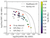 |
Fig. 2. BPT-diagram (Baldwin et al. 1981) of the sources in our Hα λ6563-subsample for which we measure [N II] λ6584. All galaxies fall in the star-forming region of the diagram. The filled and open circles have S/N([N II] λ6584) > 3 and < 3, respectively, and the 5 sources encircled in red are detected in X-rays (Luo et al. 2016). The solid and dashed curve show the AGN boundary and maximum starburst line from Kauffmann et al. (2003) and Kewley et al. (2001), respectively. |
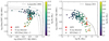 |
Fig. 3. AGN diagnostics for the sources in our Hβ λ4861-subsample, including all sources which have S/N > 3 in the relevant emission lines. Overall, our sample is consistent with star-forming galaxies. We remove one X-ray detected AGN from the sample. Left: [O II] λ3727/Hβ vs. [O III] λ4959, 5007/Hβ diagnostic from Lamareille et al. (2004), solid line, with the uncertainty indicated by the dashed lines). Right: mass-excitation diagram from Juneau et al. (2011). Galaxies in the region between the dashed and solid lines are on average identified as intermediate between AGN and SF. |
The final sample then consists of 179 star-forming galaxies, 147 from the HUDF, all with the highest redshift confidence (Inami et al. 2017), and 32 from the HDFS, between 0.11 < z < 0.91 with a mean redshift of 0.53 (see Fig. 1).
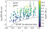 |
Fig. 1. Redshift distribution of our galaxies plotted against their (dust-corrected) SFR (1σ error bars are in grey). The colour denotes the stellar mass. The solid line depicts the lowest uncorrected SFR from Hβ λ4861 we can detect in the HUDF at each redshift (which is effectively determined by the requirement that S/N(Hγ λ4340)> 3; see Sect. 2.4). |
2.3. Stellar masses
The stellar masses of the galaxies were estimated using the Stellar Population Synthesis (SPS) code FAST (Kriek et al. 2009). The SPS-templates were χ2-fitted to the broad-band photometry of the different fields for a range of parameters. For the HUDF, we rely on the deep HST photometry from the UVUDF catalogue Rafelski et al. (2015), containing WFC3/UVIS F225W, F275W and F336W; ACS/WFC F435W, F606W, F775W, and F850LP and WFC/IR F105W, F125W, F140W and F160W) while for the HDFS we take the WFPC2 photometry from Casertano et al. (2000), F330W, F450W, F606W, and F814W). The SPS-templates were constructed from the Conroy & Gunn (2010), FSPS) models using a discrete range of metallicities (Z/Z⊙ = [0.04, 0.20, 0.50, 1.0, 1.58]). We assumed a Chabrier (2003) initial mass function with an exponentially declining star formation history (SFR ∝ exp(−t/τ) with 8.5 < log(τ/yr)< 10 in steps of 0.2 dex). The redshifts were fixed to the accurate spectroscopic values determined from the MUSE spectra. Ages were allowed to vary between 8 < logAge/yr < 10.2 in steps of 0.2 dex. We parameterised the dust attenuation curve according to the Calzetti et al. (2000) dust law with the dust extinction in the visual taken to be within 0 < AV < 3 (ΔAV = 0.1 magnitudes). For all the parameters error estimates were obtained through Monte Carlo methods, by re-running the fitting 500 times while varying the input photometry within their photometric errors (see Kriek et al. 2009 for details).
Stellar masses were determined for all 179 objects in the final sample. The distribution of masses is shown in Fig. 4. With these deep MUSE observations we are mainly probing low-mass (< 109.5 M⊙) galaxies and we can still detect star formation from emission lines in galaxies with mass ∼107 M⊙. The mass estimates with their upper and lower confidence intervals are shown for the individual objects in Fig. 7. The mean and standard deviation of the average errors on the mass estimates are 0.19 ± 0.06 dex for the HUDF and 0.22 ± 0.12 dex for the HDFS.
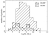 |
Fig. 4. Histograms of the stellar mass distributions of the MUSE detected galaxies in the HUDF and the HDFS. The deep 30 h observations allow us to detect and subsequently infer a stellar mass and SFR for galaxies down to ∼107 M⊙. |
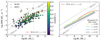 |
Fig. 7. Left panel: sample of 179 star-forming galaxies observed with MUSE, plotted on the M*-SFR plane. The symbols indicate the field and colour indicates the redshift. The dashed lines show a constant sSFR, which is equivalent to a linear relationship: SFR ∝ M*. The red curve shows the model of the star formation sequence from Whitaker et al. (2014) for 0.5 < z < 1.0. The vertical grey dashed line indicates the selection for the low-mass fit (Sect. 5.2). Right panel: same as the left panel but with the data points removed, showing (the evolution of) the star formation sequence as seen by MUSE, according to Eq. (11). |
2.4. Star formation rates
The star formation rates are inferred from the flux in the Hα λ6563 or Hβ λ4861 recombination lines emitted by H II regions, which primarily trace recent (∼10 Myr) massive star formation. Before we can infer a SFR we need to correct the measured flux in the emission lines for the attenuation by dust along the line of sight. We do this assuming a dust law according to Charlot & Fall (2000), i.e. τ ∝ λ−1.3, appropriate for birth clouds) and using the intrinsic ratio of the Balmer recombination lines (jHα/jHβ = 2.86 and jHβ/jHγ = 2.14; Hummer & Storey (1987), for an electron temperature and density of T = 10 000 K and ne = 103 cm−3). Hence, to derive an SFR(Hα λ6563) we also require a measurement of Hβ λ4861 and likewise for SFR(Hβ λ4861) we also require Hγ λ4340. After the dust correction we can convert the intrinsic flux to a luminosity using the measured redshift, given the assumed ΛCDM cosmology.
To determine the SFR we follow the treatment by Moustakas et al. (2006), which is essentially based on the relations from Kennicutt (1998). Out of the SFR indicators that MUSE has access to, the Hα λ6563 line presents the least systematic uncertainties, but it is only available at low redshifts (z ≲ 0.42 for MUSE at 9300 Å; 47 galaxies). We convert the Kennicutt (1998) relation from a Salpeter to a Chabrier IMF (0.1 < M[M⊙]< 100) by multiplying by a factor 0.62 (which is derived by computing the difference in total mass in both IMFs, while assuming the same number of massive (> 10 M⊙) stars):
 (1)
(1)
where L(Hα λ6563) is the dust-corrected luminosity. We note that this calibration assumes case B recombination and solar metallicity.
Because Hα λ6563 moves out of the optical regime at z > 0.42, the Hβ λ4861 luminosity is the primary tracer of SFR for the majority of our sample (132 galaxies). Given the intrinsic flux ratio between Hα λ6563 and Hβ λ4861, we can convert Eq. (1) into a SFR for L(Hβ λ4861):
 (2)
(2)
where L(Hβ λ4861) is corrected for dust. We note that the Hβ λ4861 derived SFR inherits all the uncertainties from SFR(Hα λ6563), including variations in dust reddening (Moustakas et al. 2006).
We also investigate the SFR using the [O II] λ3727 nebular emission line. Here we use the calibration for the Hα λ6563 SFR (Eq. (1)), where we assume an intrinsic flux ratio between [O II] λ3727 and Hα λ6563 of unity (Moustakas et al. 2006). Since [O II] λ3727 is closest to Hβ λ4861, we use the Hβ λ4861/Hγ λ4340 ratio to determine the dust correction, scaled to the appropriate wavelength. The consequence of this is that the addition of the [O II] λ3727 line as a tracer of SFR will not add any new objects to the sample. Instead, it can be used as a useful comparison, which will be discussed in Sect. 3.
To estimate the uncertainty in the SFR estimates (and dust corrections), we use Monte Carlo methods to derive a confidence interval on the SFR of every individual galaxy. We create a posterior distribution on the SFR by doing 1000 draws from a Gaussian distribution centred on the measured flux, with the variance set by the measurement error squared. The median posterior SFR can then be determined, as well as the ±1σ confidence intervals, by taking the 50th, 16th and 84th percentile from the derived posterior distribution.
3. Consistency of SFR indicators
Before turning to the results, we first consider the consistency of the derived SFRs, by comparing the SFR estimates from different tracers for the same galaxies. In the remainder of the paper we only use the dust-corrected Balmer lines as tracers of star formation.
For a significant fraction of our galaxies (≈40%) we find that the Balmer line ratios are below their case B values (as stated in Sect. 2.4), indicative of a negative dust correction. While this might seem surprising, this is not uncommon and similar ratios have been seen in spectra from, e.g. the SDSS (Groves et al. 2012), MOSDEF (Reddy et al. 2015), KBSS (Strom et al. 2017) and ZFIRE (Nanayakkara et al. 2017). While “unphysical”, these ratios are not entirely unexpected and can have several causes.
First, these deviations can be caused by noisy spectra. Most galaxies in our sample are not very dusty and hence have a ratio close to case B. In > 50% of the cases with deviant ratios, the case B ratio is indeed within the 1σ error bars. We conservatively apply no dust correction for all these galaxies. The mean dust correction for all galaxies in our sample is τ(Hβ/Hγ)≈0.6 (setting galaxies with a negative dust correction to zero) or τ(Hβ/Hγ)≈1 (including only galaxies with a positive dust correction).
Secondly, there could be a problem with the measurement. Three objects that were significantly offset from the rest of the sample showed particular problems in their emission lines. In one object (ID#971) Hγ λ4340 was severely affected by an emission line from a nearby source ([O III] λ4959 from ID#874 at z = 0.458, another galaxy in our sample, coincidentally almost exactly at the observed wavelength of Hγ). For five other objects there was a clear problem with the fit to the Hβ λ4861 (ID#894, #896, #1027) or Hα λ6563 (ID#2, #1426) emission lines. We subsequently removed the first four sources from the analysis; for the latter two we disregarded the Hα λ6563 SFR and use the Hβ λ4861 SFR.
A third, intriguing option is that theses objects are real. Indeed, there remains a small number of galaxies which have high-S/N spectra, but still show Balmer ratio’s below their case B values5. Similar objects have also been observed in the other surveys already referenced, such as SDSS (Jarle Brinchmann, priv. commun., see also Groves et al. 2012). While these are very interesting objects on their own, a detailed analysis of these sources is beyond the scope of this paper. To be conservative and consistent, we apply no dust correction for these sources.
For some objects in the sample we measure multiple emission lines, which allows us to infer a SFR from different tracers. In any case a pair of Balmer lines (either Hα/Hβ or Hβ/Hγ) is available (Sect. 2.2), to allow for a dust correction. The majority of our sample lies at z > 0.42 for which Hα λ6563 is not available, but (dust-corrected) [O II] λ3727 is available as an SFR indicator. In Fig. 5 we show a comparison for all galaxies that allowed both Hα λ6563 and Hβ λ4861 (only some galaxies at z < 0.42) and Hβ λ4861 and [O II] λ3727 derived SFRs (all redshifts). We note that Hβ λ4861 and [O II] λ3727 derived SFRs are corrected for dust using the same Hβ/Hγ-ratio.
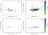 |
Fig. 5. A comparison of the derived star formation rate (SFR) from the Hα λ6563, Hβ λ4861 and [O II] λ3727 luminosities for the HUDF (top panels, circles) and the HDFS (bottom panels, triangles). Left panels: logarithm of the SFR from Hα λ6563 vs. the difference between the log Hβ λ4861 and log Hα λ6563 SFRs. Right panels: same for Hβ λ4861 vs. [O II] λ3727. In each panel σ indicates the standard deviation (in dex) around the one-to-one relation. Colour indicates the signal-to-noise ratio (S/N) in the faintest line; Hγ λ4340. Only galaxies that allowed for more than one SFR indicator are included in the plot. Overall the SFRs from Hβ λ4861 and [O II] λ3727 agree reasonably well, considering we have not taken into account the metallicity dependence in SFR([O II] λ3727). The scatter in Hα λ6563 vs. Hβ λ4861 SFR is largely driven by Hγ λ4340 S/N. |
In the right panels of Fig. 5 we see that the Hβ λ4861 and [O II] λ3727 derived SFRs agree remarkably well (standard deviation σ ≤ 0.28 dex), considering that we have not taken into account the metallicity dependence of the [O II] λ3727 luminosity in the SFR conversion factor (e.g. Kewley et al. 2004). A few points scatter quite a bit, most of which have large error bars. At lower SFRs we do see that [O II] λ3727 predicts a lower SFR than Hβ λ4861, which is probably because at low SFR we are also probing low-mass and low-metallicity galaxies. Stars with a lower metallicity have a higher UV flux, which causes the ionisation equilibrium for oxygen to shift from [O II] to [O III] which diminishes the observed [O II] λ3727 flux. Because of the opposite effect [O II] λ3727 occasionally predicts a higher SFR than Hβ λ4861 at the high-SFR end.
For a limited number of objects all three Balmer lines are in the spectral range of MUSE (0.09 < z < 0.42). We compare the Hα λ6563 and Hβ λ4861 derived SFRs in the left panel of Fig. 5, where we find reasonable agreement (in the HUDF, where we have most sources, they have a factor of ∼2 scatter). Most of the scatter is found at low SFR, where (on average) the S/N is also the lowest. In the HDFS one object (at low S/N) is a strong outlier, but removing this source yields a similar scatter to the HUDF. Intuitively the SFRs from Hα and Hβ should agree very well, which warrants some deeper investigation into the outliers at low SFR.
The main uncertainty in the SFR estimate is the amount of dust attenuation. In Fig. 6 we compare the inferred optical depth from the Hβ/Hγ-ratio (τ[Hβ/Hγ]) to the optical depth determined from the Hα/Hβ ratio (τ[Hα/Hβ]). We note though that Fig. 6 shows the measured optical depth, while we set negative τ to zero before computing the SFR. Indeed, while many sources agree well, we see that the amount of dust correction estimated from the Balmer lines is not consistent for several objects, leading to a different SFR estimate from Hα λ6563 and Hβ λ4861.
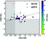 |
Fig. 6. Optical depths at the wavelength of Hβ λ4861 as derived from both the Hβ λ4861/Hγ λ4340 and the Hα λ6563/Hβ λ4861-ratio, coloured by Hγ λ4340 signal-to-noise (S/N). The dashed line is the one-to-one relation. Overall the optical depths agree reasonably well, unless the Hγ S/N is low. Most galaxies actually show little dust (τ close to zero). The shaded area shows the regions of (unphysical) negative optical depth for each axis. We set the optical depth to zero for galaxies with negative τ as this is often consistent with the error bars and the offset is due to noise in the spectra. We note that some of the high-S/N outliers actually have discrepant Balmer ratios. If the inferred optical depth is very different, this will affect the comparison of the dust-corrected SFR from Hβ λ4861 and Hα λ6563 (see Fig. 5). |
This tension is in part caused by the nature of the experiment, which requires that all three Balmer lines are in the spectral range of MUSE simultaneously. Necessarily then, Hα λ6563 will be at the long wavelength end of the spectrograph where skylines are more prevalent, occasionally adding uncertainty to its measurement. For the low-SFR sources, however, Hγ λ4340 might not be very bright, adding uncertainty to the dust correction of SFR(Hβ λ4861) for these sources (as seen at lower SFR in the left panels of Fig. 5). Indeed, most of the outliers have a low S/N in Hγ λ4340 (as stated earlier, for the objects with a negative dust correction from Hβ/Hγ, we leave the often lower S/N measurement of Hγ λ4340 out of the analysis by setting τ(Hβ/Hγ) to zero). On the other hand, the converse is not quite true: for a large number of sources with a low S/N in Hγ λ4340 we do have a consistent SFR estimate. For all objects we use the highest S/N lines available to infer a dust-corrected SFR, i.e. for objects which have a measurement of all three Balmer line we use the Hα λ6563, Hβ λ4861 pair to infer a dust-corrected SFR, which generally has the highest S/N.
In summary, we have dust-corrected SFR measurement from the Hα λ6563 and Hβ λ4861 spectral lines for all galaxies at z < 0.42 and the Hβ λ4861, Hγ λ4340-pair at higher redshifts. Comparing Hα λ6563 and Hβ λ4861 SFRs, we conclude that the dust correction is the largest uncertainty on the derived SFR. We always use the highest S/N line-pair available to compute a dust-corrected SFR. Comparing the Hβ λ4861 SFRs with [O II] λ3727 at all redshifts, we see a very consistent picture (they have ≤0.3 dex scatter in both fields). Naturally, some variations between Hβ λ4861 and [O II] λ3727 SFRs are expected given the metallicity dependent nature of [O II] λ3727.
4. Bayesian model
4.1. Definition
The star formation sequence is commonly described by a power-law relation between stellar mass (M*) and star formation rate (SFR), which evolves with redshift (z):
 (3)
(3)
where a and c are the power law exponents. It has been suggested that the slope (a) becomes shallower in the high-mass regime (M* > 1010 M⊙). In this work we will focus on the low-mass regime, for which we assume the slope is constant with mass. We will revisit this assumption in Sect. 5.2. Given the lack of homogeneous studies with redshift it is still unclear whether the low-mass slope of the relation evolves with redshift. Here, we assume that the low-mass slope is independent of redshift over the range that we probe in this study. Likewise, given the large uncertainties in (the evolution of) the intrinsic scatter, we limit the number of free parameters in the model and assume that the intrinsic scatter does not depend on any of the other model parameters.
Following this description, we model the star formation sequence by a plane in (logM*, log(1 + z), log SFR)-space:
![Mathematical equation: $$ \begin{aligned} \log {{\mathrm{SFR} }[{M_{\odot }\,\mathrm{yr}^{-1}}]} = a \log {\left(\frac{M_{*}}{M_{0}}\right)} +b + c\log {\left(\frac{1+z}{1+z_{0}}\right)}, \end{aligned} $$](/articles/aa/full_html/2018/11/aa33136-18/aa33136-18-eq8.gif) (4)
(4)
where b is now a normalisation constant. We take M0 = 108.5 M⊙ and z0 = 0.55 (close to the medians of the data) without the loss of generality. Galaxies scatter around this relation with an amount of intrinsic scatter in the vertical (i.e. log SFR) direction, which we denote by σintr. In the lack of an obvious alternative, we take the intrinsic scatter to be Gaussian in our model.
In a statistical sense we can then say that our observations (logM*, log(1 + z), logSFR) are drawn from a Gaussian distribution around the plane defined by Eq. (4). To recover this distribution, we need to take a careful approach, taking into account the heteroscedastic errors of the measurements.
We adopt a Bayesian approach to determine the posterior distribution of the model parameters (a, c, b, σintr) (see Andreon & Hurn (2010) for a lucid description of the Bayesian methodology in an astronomical context). Different approaches to construct the likelihood have been presented in the literature (see e.g. Kelly 2007 or Hogg et al. 2010). We choose to adopt a parameterisation of the likelihood following Robotham & Obreschkow (2015), hereafter R15).
First, we state that our knowledge about galaxy i (determined by the observations) is encompassed by the probability density function of a multivariate Gaussian distribution,  , with a mean value of:
 (5)
(5)
and a diagonal covariance matrix:
 (6)
(6)
containing the variance in each parameter. This is justified as both stellar mass and star formation rate are measured independently from different data. The covariance with redshift is negligible as the error on the spectroscopic redshift is very small.
Secondly, we parameterise the model given by Eq. (4) (which is a plane in three dimensions) in terms of its normal vector n, to avoid optimisation problems Robotham2015. The galaxies scatter around this plane with an amount of intrinsic Gaussian scatter, perpendicular to the plane, which we denote by σ⊥. We note that perpendicular scatter σ⊥ is distinct from the (commonly reported) vertical scatter σintr which lies in the logSFR direction. After the analysis, we can simply transform the parameters ( ) back into familiar parameters
  (using Robotham2015, Eq. (9)).
Given the above definitions, we can express our log-likelihood6 as the sum over N data points (see also Robotham2015):
![Mathematical equation: $$ \begin{aligned} \ln \mathcal{L} = -\frac{1}{2}\sum _{i=1}^{N} \left[\ln \left(\sigma _{\perp }^{2} + \frac{\boldsymbol{{n}}^{\top }C_{i}{\boldsymbol{n}}}{{\boldsymbol{n}}^{\top }{\boldsymbol{n}}}\right)+ \frac{({\boldsymbol{n}}^{\top }[{\boldsymbol{x}}_{i} -{\boldsymbol{n}}])^2}{\sigma _{\perp }^{2}{\boldsymbol{n}}^{\top }{\boldsymbol{n}} +{\boldsymbol{n}}^{\top }C_{i}{\boldsymbol{n}}} \right], \end{aligned} $$](/articles/aa/full_html/2018/11/aa33136-18/aa33136-18-eq14.gif) (7)
(7)
where all the parameters have been defined earlier.
Lastly, we have to define our priors on each component of n and on  . As we want to impose limited prior knowledge, we express our priors as uniform distributions, with large bounds compared to the typical values of the parameters (we confirm that the results are robust, irrespective of the exact choice of bounds).
 (8)
(8)
where  is the n-dimensional multivariate uniform distribution and we take into account the fact that variance is always positive.
4.2. Execution
With the likelihood and priors in hand we determine the posterior using Markov chain Monte Carlo (MCMC) methods. We use the Python implementation called emcee (Foreman-Mackey et al. 2013), which utilises the affine-invariant ensemble sampler for MCMC from Goodman & Weare (2010). emcee samples the parameter space in parallel by setting off a predefined number of “walkers”, which we take to be 250.
Following Foreman-Mackey et al. (2013), we first initialise the walkers randomly in a large volume of parameter space. We then restart the walkers in a small Gaussian ball around the median of the posterior distribution (i.e. around the “best solution”). We (generously) burn in for a quarter of the total amount of iterations for each walker which we take to be 20 000 for the main run (Sect. 5.1; roughly four hundred times the autocorrelation time). We note that for all subsequent runs described below we follow the same procedure, with similar results.
We take several steps to check whether the emcee algorithm has properly converged. As an indication, one can look at both the mean acceptance fraction of the samples as well as the autocorrelation time (Foreman-Mackey et al. 2013). For the main run the acceptance fraction that resulted from the modelling (0.45) was well within range advocated by Foreman-Mackey et al. (2013), 0.2–0.5). The autocorrelation time was also relatively short and we let the walkers sample the posterior well over the autocorrelation time. Furthermore, we confirmed that the walkers properly explored the parameter space.
Combining the results from all walkers then gives the posterior distribution over which we can marginalise to find the posterior probability distributions for the model parameters. We will discuss the results of the modelling in Sect. 5.
4.3. Model and data limitations
The unique aspect of the likelihood in Eq. (7) is that it captures both the heteroscedastic errors on the observables as well as the intrinsic scatter around the plane. Furthermore, it can simultaneously describe both the slope of the sequence as well as the evolution with redshift.
It is important to determine how well we can recover the “true” parameters with the observed data at hand. Our MUSE observations are constrained by the fact that we can only detect galaxies in a certain redshift range and cannot detect galaxies below the flux limit of the instrument (see Fig. 1). As the flux limit varies with redshift, this could introduce a bias in our inferred parameters. The reason behind this is that the lack of low-SFR galaxies at higher redshift will bias the posterior towards shallower slopes, with a steeper redshift evolution (see Fig. A.1 for an illustration). In order to correct for such a bias, we analyse a series of simulated observations. We briefly outline the procedure here, which is described in detail in Appendix A.
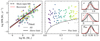 |
Fig. A.1. Results from the recovery experiment on mock galaxies. The points in the left and centre panels show one of the 30 realisations of 100 galaxies in (log M*, log(1 + z), log SFR)-space from a mock star formation sequence: logSFR ∝ alogM* + clog(1 + z), where in this particular case a = 0.8 and c = 2.0 with σintr = 0.5 dex. The colour indicates redshift, unless a mock galaxy falls below the solid line in the centre panel, indicating the flux limit of ∼3 × 10⁻¹⁹ erg s−1 cm−2, in which case it is a black point. The rightmost panels show the marginalised distributions (slope, redshift evolution, and intrinsic scatter) from combining all 30 realisations for this particular set of parameters. The thin and thick black lines indicate the results when taking into account all mock data and only the data above the flux limit, respectively, and are compared to the input values (dashed lines). With all data points (including noise), we can recover the input parameters sequence well. When applying the flux limit a slight bias towards a shallower slope and steeper redshift evolution appears. We plot all curves in the leftmost panel at the average redshift of the sample (z0). The red line is obtained after applying the correction to the fit of the data above the limit. These recovered curves are plotted in the leftmost panel as well and compared to the input mock relation. With our correction, we can recover the true input parameters well, even in the case of limited data. |
In order to characterise the bias in the inferred parameters, we simulate galaxies from a mock star formation sequence for a range of values in each parameter, which we call xtrue, k (see Table A.1). After applying the redshift-dependent flux limit to the mock data, we model the remaining galaxies as described in Sect. 4 and recover the parameters, xout, k. We then fit the transformation between the true and recovered parameters with an affine transformation (xout, k = Axtrue, k + b) as outlined in Sect. A.2. The inverse of the best-fit transformation (Eq. (A.3)) can then be used to correct the posterior density distribution as measured from the MUSE data. In the following, we provide both the uncorrected (directly fitted) and the corrected values for reference.
5. Star formation sequence
5.1. Global sample
With a reliable SFR estimate in hand, we can turn to the star formation sequence between 0.11 < z < 0.91 as observed by MUSE. Fig. 7 shows a plot of stellar mass (M*) versus star formation rate (SFR) for all the galaxies in the sample. The figure is based on two dust-corrected SFR indicators: the Hβ λ4861 and Hα λ6563 luminosities (Eqs. (2) and (1)). The vertical grey lines indicate the errors in (logM*, log SFR) for each of the individual galaxies. The mean average error on the SFR is ≈0.2 dex in both the HUDF and the HDFS.
We are able to detect star formation in galaxies down to star formation rates as low as  . The galaxies appear to follow the M*-SFR trend closely over the complete mass range, down to the lowest masses we can probe here ∼107 M⊙. At the high-mass end it appears we are starting to witness a flattening off of the trend, although we are primarily sensitive to the intermediate and low-mass galaxies.
We model the M*-SFR relation with the Bayesian MCMC methodology described in detail in Sect. 4. We show the resulting posterior probability density distribution for the parameters in Fig. 8. By marginalising over the various parameters, we recover the posterior probability distributions for the individual parameters of interest (a, c, b, σintr). These are plotted as histograms above the various axes in Fig. 8. By taking the median and the 16th and 84th percentile from the posterior distributions we derive the median posterior value and a 1σ confidence interval for the parameters of interest.
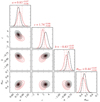 |
Fig. 8. Projections of the 4D posterior distribution for the model parameters: slope (a), evolution (c), normalisation (b) and intrinsic scatter (σintr). The histograms on top show the marginalised distributions of the model parameters. The bias-corrected posterior median value and the 16th and 84th percentile are denoted by the dashed lines and by the values above the histograms. The contours show the 0.5, 1, 1.5 and 2σ levels. The posterior directly from the modelling is shown in black, red indicates the posterior after applying the bias correction (Eq. (A.3)). Figure created using the corner.py module (Foreman-Mackey 2016). |
The (uncorrected) best-fit (i.e. median posterior) parameters of the distribution (with their confidence intervals) that describe the star formation sequence are:
![Mathematical equation: $$ \begin{aligned} \log {\mathrm{SFR} }[{M_{\odot }\,\mathrm{yr}^{-1}}] =\;&{0.79^{+0.05}_{-0.05}}\log \left(\frac{M_*}{M_{0}}\right) {-0.77^{+0.04}_{-0.04}}\nonumber \\&+ {2.78^{+0.78}_{-0.78}}\log \left(\frac{1+z}{1+z_{0}}\right) \pm {0.46^{+0.04}_{-0.03}}, \end{aligned} $$](/articles/aa/full_html/2018/11/aa33136-18/aa33136-18-eq24.gif) (9)
(9)
analogous to Eq. (4). The final term represents the intrinsic scatter  in the vertical (logSFR) direction. We note that while it is a perfectly valid option for the parameterisation of the likelihood, the posterior distribution does not favour models with zero intrinsic scatter.
Figure 8 shows that some correlations exist between the different parameters of the model, which is expected. The strongest correlation exists between slope and redshift evolution as a less steep slope requires more evolution in the normalisation to be compatible with the data. The complete covariance matrix between the different parameters is:
 (10)
(10)
We correct the posterior for observational bias, by applying Eq. (A.3), which is indicated by the red contours in Fig. 8. This yields a steeper slope, with a significantly shallower redshift evolution:
![Mathematical equation: $$ \begin{aligned} \log {\mathrm{SFR} }[{{M_{\odot }}\,{\mathrm{yr}}^{-1}}] =\;&0.83^{+0.07}_{-0.06}\log \left(\frac{M_*}{M_{0}}\right) {-0.83^{+0.05}_{-0.05}}\nonumber \\&+ {1.74^{+0.66}_{-0.68}}\log \left(\frac{1+z}{1+z_{0}}\right) \pm {0.44^{+0.05}_{-0.04}}, \end{aligned} $$](/articles/aa/full_html/2018/11/aa33136-18/aa33136-18-eq27.gif) (11)
(11)
At the same time, the transformation has little effect on the intrinsic scatter. The covariance in the corrected posterior is essentially the same as the uncorrected one, with a slight increase in covariance with intrinsic scatter.
 (12)
(12)
We compare the generative distribution (i.e. Eq. (9)) with the data in Fig. 9. As the plane is three dimensional, we show a projection where we have subtracted the evolution with redshift from the y-axis. Overall, the distribution appears to describe the data very well and the scatter in the observations has tightened with respect to Fig. 7. For a more familiar representation we also show the resulting star formation sequence in the right panel of Fig. 7, for a number of different redshifts.
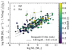 |
Fig. 9. The best-fit star formation sequence for the 179 star-forming galaxies observed with MUSE. The symbols indicate the dust-corrected tracer used to infer the SFR. The solid line shows best-fit relation, as presented in Eq. (11), and the dashed lines show the 1σ intrinsic scatter. We subtract the evolution from the y-axis and scale to the average redshift of the sample; z = 0.55. After accounting for evolution, the galaxies clearly follow the star formation sequence, down to the lowest masses and SFRs. The slightly larger fraction of galaxies that scatter into the high-mass, low-SFR regime may be a result of the flattening of the relation above M* = 1010 M⊙. |
5.2. Low-mass sample (log M* [M⊙] < 9.5)
We are primarily interested in the low-mass end of the star formation sequence. Our deep MUSE sample spans a significant mass range, between log M*[M⊙]=6.5 − 11. As several studies have suggested different characteristics for the star formation sequence above and below a turnover mass of M* ∼ 1010 M⊙ (e.g. Whitaker et al. 2014; Lee et al. 2015; Schreiber et al. 2015), we repeat the above analysis excluding galaxies above a certain mass threshold. To be on the conservative side, we choose this mass threshold to lie at M* = 109.5 M⊙. This excludes 31/179 ≈ 17.5% of the sample. We include this threshold as a dashed vertical line in Fig. 7. We then repeat the modelling identically to what has been described in the previous sections.
The bias-corrected star formation sequence for galaxies that have a stellar mass below M* < 109.5 M⊙ is:
![Mathematical equation: $$ \begin{aligned} \log {\mathrm{SFR} }[{M_{\odot }\,\mathrm{yr}^{-1}}] =\;&{0.83^{+0.10}_{-0.09}}\log \left(\frac{M_*}{M_{0}}\right) {-0.79^{+0.05}_{-0.05}}\nonumber \\&+ {2.22^{+0.75}_{-0.76}}\log \left(\frac{1+z}{1+z_{0}}\right) \pm {0.47^{+0.06}_{-0.05}}. \end{aligned} $$](/articles/aa/full_html/2018/11/aa33136-18/aa33136-18-eq29.gif) (13)
(13)
The result is essentially the same, with the main difference being a steeper redshift evolution. All parameters are within errors consistent with the relation for our complete sample (also for the uncorrected values, see Table 1). This reflects the fact that we are primarily sensitive to the low-mass end of the galaxy sequence. As this fit utilises only a part of the data we will refer primarily to the fit based on all the data, Eq. (11), as the main result in the remainder of the paper. We report the (un)corrected values for all the fits in Table 1.
Star formation sequence parameters for different samples.
5.3. The effect of redshift bins (2D)
Most previous studies have not modelled the redshift evolution of the star formation sequence directly, but have instead divided the data into redshift bins and adopted a non-evolving relation: logSFR = a log M* + b. To facilitate the comparison with the literature, we adapt our model to fit the relation in the (logM* log SFR)-plane, without taking the redshift evolution into account. This is easily done, by taking a two-dimensional version of our likelihood, disregarding the second, log(1 + z)-component in Eqs. (5)–(8) – the rest of the modelling is be identical. We note that we still take both heteroscedastic errors as well as intrinsic scatter into account (see Sect. 4.1), however, we do not apply the bias correction.
We model both the entire redshift range, as well as the 0.1 < z < 0.5 and 0.5 < z < 1.0 range separately (similar to other studies). The results are collected in Table 1. For the full sample the slope is significantly steeper than when we take into account the redshift evolution, when comparing to our uncorrected fits:
![Mathematical equation: $$ \begin{aligned} \log {\mathrm{SFR} }[{M_{\odot }\,\mathrm{yr}^{-1}}]= {0.89^{+0.05}_{-0.05}}\log \left(\frac{M_*}{M_{0}}\right) {-0.82^{+0.04}_{-0.04}}. \end{aligned} $$](/articles/aa/full_html/2018/11/aa33136-18/aa33136-18-eq57.gif) (14)
(14)
This is also the case for the smaller samples in both redshift bins, although the results are consistent with Eq. (9) within the error bars (which are larger due to lower number statistics). The resulting relations are
![Mathematical equation: $$ \begin{aligned} \log {\mathrm{SFR} }[{M_{\odot }\,\mathrm{yr}^{-1}}] = {0.86^{+0.09}_{-0.08}}\log \left(\frac{M_*}{M_{0}}\right) {-0.92^{+0.07}_{-0.07}}, \end{aligned} $$](/articles/aa/full_html/2018/11/aa33136-18/aa33136-18-eq58.gif) (15)
(15)
for 0.1 < z ≤ 0.5 and
![Mathematical equation: $$ \begin{aligned} \log {\mathrm{SFR} }[{M_{\odot }\,\mathrm{yr}^{-1}}] = {0.84^{+0.07}_{-0.06}}\log \left(\frac{M_*}{M_{0}}\right) {-0.73^{+0.06}_{-0.06}}\end{aligned} $$](/articles/aa/full_html/2018/11/aa33136-18/aa33136-18-eq59.gif) (16)
(16)
for 0.5 < z < 1.0.
Given the significant evolution we found in the star formation sequence with redshift, this result is expected. While incidently these slopes are similar to our corrected fits, we caution that this does not imply that not modelling the redshift evolution can circumvent biases introduced by flux-limited observations.
6. Discussion
We have modelled the star formation sequence down to 108 M⊙ at 0.11 < z < 0.91 using a Bayesian framework (Sect. 4) that takes into account both the heteroscedastic errors on the observations as well as the intrinsic scatter in the relation. One major advantage of our framework is that we simultaneously model both the slope and the evolution in the M*-SFR relation, while most previous studies have modelled these separately by dividing their sample into different redshift bins. As demonstrated in Sect. 5.3, these results are not necessarily consistent, which can be attributed to evolution taking place within a single redshift bin. Another important difference is that we use the Balmer lines to trace the (dust-corrected) star formation, while most other recent studies have relied on SFRs derived from UV+IR/SED-fitting, using different dust corrections (Whitaker et al. 2014; Lee et al. 2015; Schreiber et al. 2015; Kurczynski et al. 2016).
As described in Sect. 5.1, we have found that the star formation sequence (shown in Figs. 7 and 9) is well described by Eq. (11) (see also Table 1). We now compare our results to other literature measurements and discuss each aspect of the star formation sequence separately, i.e. the redshift evolution, intrinsic scatter and the slope. We focus particularly on the slope, for which we find the strongest constraints, and continue with a discussion of the physical implications of our results.
6.1. Comparison with the literature
6.1.1. Evolution with redshift
We find that the normalisation in the star formation sequence increases with redshift as (1 + z)c with  (
( for M* < 109.5 M⊙). The fact that the normalisation of the star formation sequence increases with redshift is well known and attributed to the change in cosmic gas accretion rates and gas depletion timescales. Most studies have probed the higher mass regime and report values in the range of sSFR ≡ SFR/M* ∝ (1 + z)2.5 − 3.5 at 0 < z < 3 (e.g. Oliver et al. 2010; Karim et al. 2011; Ilbert et al. 2015; Schreiber et al. 2015; Tasca et al. 2015). Looking specifically at the low-mass regime, Whitaker et al. (2014) reports sSFR ∝ (1 + z)1.9, similar to our result. Their more massive end indeed shows stronger evolution sSFR ∝ (1 + z)2.2 − 3.5. Lee et al. (2015) on the other hand, find much steeper evolution, with sSFR ∝ (1 + z)4.12 ± 0.1. We note that our parameterisation assumes a power-law type of evolution of the star formation sequence with redshift. We have decided to stick to this very common first-order approximation. Still, one should keep in mind that a more complex evolution with redshift is possible, both non-linear in time as well as a different evolution in different mass regimes. We do not find strong constraints on the redshift evolution due to our relatively small redshift range from z = 0.1 to z = 0.91. Still, the results from Sect. 5.3 show that it is important to take the redshift evolution into account, in order to get a robust constraint on the slope.
6.1.2. Intrinsic scatter
Constraining the intrinsic scatter in the star formation sequence has proven to be challenging as one has to separate the intrinsic scatter from the measurement error (e.g. Noeske et al. 2007b; Salim et al. 2007; Salmi et al. 2012; Whitaker et al. 2012; Guo et al. 2013; Speagle et al. 2014; Schreiber et al. 2015). This challenge in particular motivates our adopted model, which directly constrains the amount of intrinsic scatter in the relationship, even in the presence of measurement errors. Meanwhile, our measurements are not affected by binning, e.g. we do not boost the scatter artificially because of evolution of the star formation sequence within a single bin.
In our best fit model we find  dex, which is larger than the value of ∼0.2 − 0.4 dex that is commonly found (e.g. Speagle et al. 2014; Schreiber et al. 2015). Kurczynski et al. (2016) determined an intrinsic scatter of σintr = 0.427 ± 0.011 in their lowest redshift bin (0.5 < z < 1.0) in the HUDF, similar to our result, but found significantly smaller scatter at higher redshifts. They determined the intrinsic scatter by decomposing the total scatter (σTot = 0.525) using the covariance matrix between M* and SFR determined from their SED fitting.
There are several effects that could potentially affect the scatter. Measurement outliers are not a cause of concern for the intrinsic scatter as they are taken into account by the likelihood approach. However, if galaxies are included in the sample that are not on the M*-SFR relation, such as red-sequence galaxies or starbursts, then these might artificially increase the scatter. We argue that the former is unlikely as our selection criteria based on the 4000 Å break and the Hα λ6563 or Hβ λ4861 equivalent width effectively remove all red-sequence galaxies from the sample. On the other hand, our sample does include a small number of galaxies that are offset from the relation towards high SFRs. We verified however that removing all galaxies with a sSFR > 10 Gyr−1 from the sample does not significantly increase or decrease the scatter.
Hypothetically, if the error bars on the SFR are underestimated, this will artificially boost the intrinsic scatter in the relationship. To determine the influence of the size of the error bars we redid the modelling while folding in an additional error on the SFR of 0.2 dex in quadrature (effectively doubling the average error bars); this decreased the scatter by 20% to ∼0.4 dex. The sample size does not seem to affect the measurement and splitting our sample did not yield significantly larger scatter (see Sect. 5.3).
Assuming our measured scatter is real, it might be that previous studies have underestimated the amount of intrinsic scatter. One potential danger might lie in the derivation of both stellar mass and SFR from the same photometry. Especially in SED modelling this might introduce correlations between M* and SFR as both are regularised through the same star formation history in the model spectrum which could artificially decrease the scatter.
More physically, the difference could also in part be due to the fact that the Balmer lines trace the SFR on shorter timescales (stars with ages ≤10 Myr and masses > 10 M⊙) than the UV does (ages of ≤100 Myr and masses > 5 M⊙; e.g. Kennicutt 1998; Kennicutt & Evans 2012). Simulations have indeed found that SFRs averaged over timescales decreasing from 108 to 106 yr could be significantly larger (Hopkins et al. 2014; Sparre et al. 2015), particularly if star formation histories are bursty (e.g. Dominguez et al. 2015; Sparre et al. 2017).
Furthermore, as the recent star formation histories of low-mass galaxies are more diverse, it can be expected that there is more scatter in the star formation sequence at low stellar masses. This indeed has been predicted by simulations (e.g. Hopkins et al. 2014; Sparre et al. 2017) as well as semi-analytical models (e.g. Mitra et al. 2017). Observing such a trend requires a large and highly complete sample of galaxies over an extended mass range and hence evidence has been inconclusive. Using a large sample of galaxies from the SDSS, Salim et al. (2007) reported a decrease in the scatter of −0.11 dex−1 from 108 to 1010.5 M⊙, but such a trend with mass has not been confirmed by studies at higher masses (Whitaker et al. 2012; Guo et al. 2013; Schreiber et al. 2015; Kurczynski et al. 2016). Recently though, Santini et al. (2017) have found indications of decreasing scatter with mass in the Frontier Fields, albeit at higher redshifts (z > 1.3).
A large and complete sample of galaxies, covering the (logM*, log SFR, log(1 + z))-space, with independent stellar mass and SFR estimates, is required to get a firm handle on the intrinsic scatter in the star formation sequence.
6.1.3. Slope
We find a best-fit (median posterior) slope of the star formation sequence of  (log SFR ∝alogM*). This slope is determined from galaxies that are more than an order of magnitude lower in mass than most earlier studies at z > 0, i.e. at 108 − 1010 M⊙, whereas most previous studies (e.g. Speagle et al. 2014; Lee et al. 2015; Schreiber et al. 2015) have been primarily sensitive to a higher mass range from 109.5 M⊙ to 1011 M⊙. For reference, we plot the polynomial fit from Whitaker et al. (2014) (down to their mass completeness limit, based on stacking) in Fig. 7.
Recent studies have typically observed a shallower slope at the high-mass end, i.e. above 1010 M⊙ (e.g. Whitaker et al. 2014). Gavazzi et al. (2015) find a turnover mass of M* ∼ 109.7 M⊙ at z = 0.55 (after converting their result to a Chabrier IMF), increasing with redshift. As discussed in Sect. 5.2, excluding galaxies above M* > 109.5 M⊙ has no significant effect on the slope. Only 15/179 ≈ 8.5% of galaxies in our sample have M* > 1010 M⊙ and thus our result is not very sensitive to this turn-over. In light of this, we limit the following discussion to studies which specifically probe the mass range below the turnover of the star formation sequence.
Our best-fit slope of  is compared to the values found by other recent studies in Fig. 10 where we focus on studies with similar redshift ranges (i.e. 0 < z < 1) and which extend well below M* < 1010 M⊙. The slope in this regime is notably steeper than the consensus relation from Speagle et al. (2014) who reported a = 0.6 − 0.7 at our redshifts, due to the fact that this compilation is for a mass range of log M*[M⊙]=9.7 − 11.1, where the slope is significantly shallower. Our slope is shallower than the low-mass power-law slope from Whitaker et al. (2014), a = 0.94 ± 0.03 for M* < 1010.2 M⊙) from the 3D-HST catalogues in CANDELS, but is consistent with the global slope of a = 0.88 ± 0.06 reported by Lee et al. (2015) in a large sample of star-forming galaxies in COSMOS. Kurczynski et al. (2016) have also presented a characterisation of the star formation sequence in the HUDF, based on the CANDELS/GOODS-S (Santini et al. 2015) and UVUDF (Rafelski et al. 2015) catalogues. In their lowest redshift bin (0.5 < z < 1.0), which goes down to M* ∼ 107.5 M⊙ they find a slope of a = 0.919 ± 0.017, which is also steeper (marginally consistent) compared to what find. We note that they determined both masses and SFRs from the SED modelling, taking into account the correlations between the parameters, as their study was focused particularly on measuring the intrinsic scatter, see Sect. 6.1.2. In the same field Bisigello et al. (2018) find a slope of 0.9 ± 0.01 (0.5 ≤ z < 1.0), after selecting galaxies with log sSFR[Gyr−1] < −9.8.
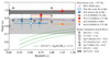 |
Fig. 10. A comparison of the slope (a) as a function of redshift (z) with studies from the literature that extend down to M* < 1010 M⊙ near our redshift range. Our best-fit (bias-corrected) slope from Eq. (11) is shown by the large star. As most studies have probed the slope in bins of redshift, we also include our results obtained using non-evolving redshift bins (Eqs. (14), (15) and (16); smaller blue stars). The literature results are from Renzini & Peng (2015), RP15),Kurczynski et al. (2016), K16), Bisigello et al. (2018), B18) and the low-mass (M* ≲ 1010 M⊙) power-law slopes from Whitaker et al. (2014), W14) and Lee et al. (2015), L15). We also add [SP14],Speagle2014 for reference, though it is inferred at higher masses. We indicate the field and SFR-tracer in brackets, though note that distinct calibrations for the same tracer may be used in different studies. In addition, we add the slopes predicted by (semi-)analytical models; Bouché et al. (2010), B10), Mitchell et al. (2014), M14), Mitra et al. (2015), Mi15), Cattaneo et al. (2017), C17), and hydrodynamical simulations; Sparre et al. (2015), Sp15), Furlong et al. (2015), F15), Sparre et al. (2017), Sp17). |
The Sloan Digital Sky Survey (SDSS; York et al. 2000; Abazajian et al. 2009) serves as a natural reference for Balmer line-derived SFRs in the local universe and since Brinchmann et al. (2004) different studies have derived the star formation sequence slope (e.g. Salim et al. 2007; Elbaz et al. 2007). The most recent of these is Renzini & Peng (2015), who measure the slope of the ridge line in the M* − N × SFR-plane (where N is the number of galaxies in every M*-SFR bin) and find a = 0.76 ± 0.01, which is significantly flatter than our results.
Taken at face value, our slope of  is inconsistent with a linear slope (a = 1). A value (close to) unity may have been expected on the basis of simulations (see next section), which is also evident from the fact that several parameterisations of the star formation sequence asymptote to a linear relation at low mass (e.g. Schreiber et al. 2015; Tomczak et al. 2016). An independent motivation for a near-linear value comes from the fact that there is very little evolution in the faint slope of the stellar mass function of star-forming galaxies up to z = 2 (see, e.g. Tomczak et al. 2014; Davidzon et al. 2017 for recent results). To first order, this may implies self-similar mass growth for low-mass galaxies (i.e. constant sSFR which implies a linear slope for the star formation sequence), unless balanced by mergers (Peng et al. 2014). Leja et al. (2015) investigated the link between the slope of the star formation sequence and the stellar mass function. While they do not provide precise constraints on the low-mass slope at low redshift (due to the challenge of disentangling growth through star formation and mergers), their results indicate that a sub-linear low-mass slope is still consistent with the stellar mass functions at z < 1.
6.1.4. Evolution of the low-mass slope
Combining results from the local universe out to redshift z ∼ 6, Speagle et al. (2014) found evidence for an evolving slope at the high-mass end (M* > 109.7 M⊙), where the slope gets shallower with redshift (cf. Abramson et al. 2016, Fig. 5). Given the turnover in the star formation sequence at high mass, it is important to disentangle to what extent the evolution in the slope is due to different studies being sensitive to distinct mass regimes. Our data are too sparse in redshift space to simultaneously constrain the evolution of the slope (and hence we have adopted a single power-law slope for the sequence).
In light of the potential redshift evolution of the slope, we plot the slope as a function of redshift in Fig. 10, compared to literature results which probe the mass range M * < 1010 M⊙ at z < 1.5. Figure 10 provides evidence for evolution of the low-mass slope with redshift. However, we caution against a too strong interpretation of such a trend as the literature suffers from studies probing distinct mass ranges (sometimes including the turn-over regime). What further complicates a fair comparison is that different tracers of star formation probe different timescales and additionally use varying dust corrections, which are not necessarily consistent (e.g. Davies et al. 2016). A consistent analysis of the low-mass galaxy population out to higher redshifts is important to quantify potential evolution in the low-mass slope.
6.2. The MS slope – a quantitative comparison to models
The galaxy main sequence (MS) is a natural outcome of hydrodynamical models (e.g. Fig. 1b in Bouché et al. 2005; Davé 2008; Genel et al. 2014; Torrey et al. 2014; Kannan et al. 2014; Hopkins et al. 2014; Sparre et al. 2015; Furlong et al. 2015) and in semi-analytical models (e.g. Somerville et al. 2008; Dutton et al. 2010; Cattaneo et al. 2011, 2017; Mitchell et al. 2014; Henriques et al. 2015; Hirschmann et al. 2016). These models have reported a slope (and scatter) that, in general, is broadly consistent with observations, but the quantitative details regarding the slope and/or the evolution of the main sequence often do not match observations.
Since the pioneering work of Daddi et al. (2007) and Elbaz et al. (2007), it has been noted that the redshift evolution of the main sequence normalisation, in particular around z = 2, is a challenge for models (e.g. Davé 2008; Damen et al. 2009; Bouché et al. 2010; Dutton et al. 2010; Dekel & Mandelker 2014; Torrey et al. 2014; Genel et al. 2014; Mitchell et al. 2014; Furlong et al. 2015; Sparre et al. 2015; Abramson et al. 2016; Santini et al. 2017). Here, we focus on a quantitative comparison of the slope of the main sequence (SFR ∝  ) with various models, given that our study yields the tightest constraint on this parameter (compared to the other parameters in the model).
The Illustris simulations (Vogelsberger et al. 2014; Genel et al. 2014; Sparre et al. 2015) produce a main-sequence with a slope a that is slightly sub-linear with a ⪅ 1.0. In particular, Genel et al. (2014) noted that sSFR goes as ≃ − 0.1 with stellar mass and using the results from Sparre et al. (2015), we find that the main sequence in Illustris goes as  . The EAGLE simulations (Schaye et al. 2015; Crain et al. 2015) also allow an investigation of the main sequence and Furlong et al. (2015), their Fig. 5), showed that the sSFR is constant with M* from 108 to 1010 M⊙ at redshifts z = 0.1, 1.0 and 2.0, with a relatively steep decline above 1010 M⊙. Quantitatively, below 1010 M⊙, the slope of the main sequence a in Furlong et al. (2015) is a ≈ 1.04. The MS slope for the Illustris and EAGLE simulations are shown in Fig. 10 as the open circles and triangle symbols, respectively. In the FIRE simulations (Hopkins et al. 2014), Sparre et al. (2017) focused on studying the scatter in the main sequence for different tracers of SFR and shows a slope of a ≈ 0.98 when using the FUV (their Fig. 2).
The MS slope has also been a challenge for semi-analytical models because different (regular) feedback prescriptions do not alter the MS slope as shown in Dutton et al. (2010) and discussed in Mitchell et al. (2014), however, it can alter the slope in hydrodynamical simulations, e.g. Haas et al. 2013a, b; Crain et al. 2015). Mitchell et al. (2014) performed a detailed comparison between predictions from the GALFORM semi-analytical models with observations and their fiducial model produces a MS slope of a ≈ 0.85 (shown in Fig. 10 as the down-pointing triangles). Recently, the semi-analytical model of Cattaneo et al. (2017) using the GALICS2 code was set to reproduce the local luminosity function and the local MS slope simultaneously. Their MS slope is a ≈ 0.8 (open square in Fig. 10), but we caution their use of an extreme feedback model, where the mass loading η is η ∝ V−6, where V is the halo virial velocity. Such a steep scaling between galaxy mass and wind loading is not supported by the data (e.g. Schroetter et al. 2016).
Bouché et al. (2010) used a simple toy model for galaxy (self-)regulation with which they showed that variations in feedback prescriptions or in the laws of star formation have no impact on the MS slope. They argued that while ejective feedback alone is not sufficient to bring the theoretical slope of the main-sequence in agreement with observations, preventive feedback can easily do so as several studies have shown (Davé et al. 2012; Lu et al. 2015; Mitra et al. 2015, 2017). However, while the MS slope of Bouché et al. (2010) is sub-linear with a ≈ 0.8, a quantitative analysis reveals that the slope varies rapidly with stellar mass, likely due to the limitations of the model. Indeed, the MS slope of Bouché et al. (2010) goes from 0.7 at M* ∼ 109.5 M⊙ to 0.9 at M* ∼ 1010.5 M⊙. The range of values is indicated by the light grey box in Fig. 10.
Mitra et al. (2015) expanded the self-regulation model of Bouché et al. (2010),Davé et al. (2012), and others) with physically motivated parameters and attempted to determine these parameters using a Bayesian MCMC approach on a set of observed scaling relations at 0 < z < 2. Their fiducial model yields a MS with a slope that is quasi-linear with a ∼ 0.95 in our mass regime, i.e. below 1010 M⊙. Their MS slope is shown as the dark grey band in Fig. 10.
Generally speaking, in the low-mass regime below 1010 M⊙, hydrodynamical simulations have steeper MS slopes with a ≈ 1.0 whereas our estimate ( ) at z < 1 and recent observations covering that mass range indicate a < 1.0 (see Fig. 10). The reason that models tend to predict a steeper main sequence slope lies in the underlying feature in hydrodynamical simulations and semi-analytical models, where the growth rate for dark matter halos
  scales with mass as
  (Birnboim et al. 2007; Genel et al. 2008; Dekel et al. 2009; Fakhouri & Ma 2008; Neistein & Dekel 2008), in combination with rapid gas cooling.
6.3. Implications of a shallow slope
As noted originally by Noeske et al. (2007a) and discussed in Mitchell et al. (2014) and Abramson et al. (2016), a MS with a sub-linear slope,  with a < 1, implies downsizing where lower-mass galaxies have longer e-folding time and a later onset of star formation. This downsizing effect would be amplified if the MS slope is substantially flatter above 1010 M⊙ as some studies have indicated (Whitaker et al. 2014; Schreiber et al. 2015; Lee et al. 2015; Tomczak et al. 2016). This turnover has generally been attributed to either a morphological transition, such as bulge growth (Abramson et al. 2014; Lee et al. 2015; Whitaker et al. 2015), or a reduced star formation efficiency (Schreiber et al. 2016).
Our result, that the slope of the main sequence is sub-linear in the low-mass regime, implies that there are processes at work which either: (1) affect the conversion of the accreted gas into stars through increased (supernova) feedback or a decrease in the SF efficiency; or (2) prevent the accretion of gas onto low-mass galaxies. These two processes might conspire with the fact that the gravitational potential is shallower in low-mass galaxies (Mitra et al. 2015).
In hydrodynamical simulations low-mass galaxies (up to halo masses of ∼1011.5 M⊙) obtain their gas primarily through “cold”-accretion (Kereš et al. 2005; Van de Voort et al. 2011), where the gas is never heated to the virial temperature, while “hot” accretion, where gas is first shock heated to the virial temperature and then cools and accretes, is dominant for more massive galaxies. A candidate process is feedback from gravitational heating, due to the formation of virial shocks (e.g. Faucher-Giguère et al. 2011), which becomes more effective at higher masses, however, can still play a role down to halo masses of 1010 M⊙. The heating of gas through winds (from either supernovae or black hole feedback) can also prevent the gas from flowing into the galaxy (Oppenheimer et al. 2010; Faucher-Giguère et al. 2011; Van de Voort et al. 2011), in particular in low-mass galaxies. However, Schaye et al. (2010) pointed out that this type of feedback mainly has a regulatory effect on the gas infall.
As noted by Dutton et al. (2010), Bouché et al. (2010), and Mitchell et al. (2014), in semi-analytical models, the MS slope is rather insensitive to the ejective (regular) feedback mechanisms7, such as the heating of gas through winds and/or the star formation efficiency (Kennicutt 1998) because they act primarily on the gas content. Hence, the SFR and stellar mass are affected in a similar way, leaving the slope unchanged, unless the ejective feedback prescription is strongly mass dependent with η ∝ V−6, as in Cattaneo et al. (2017). In addition, Mitchell et al. (2014) showed that the slope is also insensitive to the gas re-incorporation prescription (see also Mitra et al. 2015).
Preventive processes (Blanchard et al. 1992; Gnedin 2000; Mo et al. 2005; Lu & Mo 2007; Okamoto et al. 2008) that tend to be mass dependent can more easily impact the MS slope, the Tully-Fischer relation, and the luminosity function as argued by Bouché et al. (2010). A preventive process which can prevent the inflow of gas specifically in low-mass halos is photoionisation heating (Quinn et al. 1996). While it has been argued that this process is primarily effective in dwarf galaxies and becomes ineffective above halo masses of a few times 109 M⊙ (e.g. Okamoto et al. 2008), Cantalupo (2010) suggest that photoionisation may still play a role for more massive halos if there is significant star formation.
7. Summary and conclusions
We have exploited the unique capabilities of the MUSE instrument to investigate the star formation sequence for low-mass galaxies at intermediate redshift (0.11 < z < 0.91). From the large number of sources detected with MUSE in the HUDF and HDFS we have constructed a sample of 179 star-forming galaxies down to M* ∼ 108 M⊙, with a number of objects at even lower masses (Fig. 4). The accurate spectroscopic redshifts from MUSE are combined with the deep photometry available over the HUDF and HDFS to determine a robust mass estimate for the galaxies in our sample through stellar population synthesis modelling.
With MUSE we can detect star-forming galaxies down to SFR  (Fig. 7). We show that we can determine robust, dust-corrected SFR estimates from Hα λ6563 and Hβ λ4861 recombination lines, by comparing the SFRs from different tracers (Fig. 5). A dust-corrected star formation rate is inferred from the Hα λ6563 and Hβ λ4861 emission lines observed with S/N > 3 in the MUSE spectra.
We characterise the star formation sequence by a Gaussian distribution around a plane (Eq. (4)). This methodology is chosen to maximally exploit the data set taking into account heteroscedastic errors. We constrain the slope, normalisation, intrinsic scatter, and evolution with redshift from the posterior probability distribution via MCMC methods (Fig. 8).
We analyse the robustness of our model and the influence of the MUSE detection limit on the derived properties of the star formation sequence, by determining how well we can recover the parameters from a sample of simulated relations (detailed in Appendix A). Using the results, we correct our inferred parameters for observational biases.
We report a best-fit description of the low-mass end of the galaxy star formation sequence of  between 0.11 < z < 0.91, shown in Fig. 9. The full description of our parameters, including errors and normalisation, is found in Eq. (11).
The intrinsic scatter around the sequence is found to be  dex (in log SFR). This is notably higher than the average value reported in literature (∼0.3 dex), which could be attributed to a combination of the Balmer lines probing star formation on shorter timescales and the star formation histories of low-mass galaxies being more diverse.
Excluding massive galaxies (with M* > 109.5 M⊙) has no significant effect on the best-fit parameters, indicating we are primarily sensitive to low-mass galaxies. Notably though, we find that the slope steepens when splitting our sample into one or multiple redshift bins, with the values going up to ![Mathematical equation: $ \log{\mathrm{SFR}}[{M_{\odot}\,\mathrm{yr}^{-1}}] = {0.89^{+0.05}_{-0.05}} \log{M_{*}}[M_{\odot}] $](/articles/aa/full_html/2018/11/aa33136-18/aa33136-18-eq75.gif) . This shows the importance of taking into account the evolution with redshift when deriving the properties of the star formation sequence.
. This shows the importance of taking into account the evolution with redshift when deriving the properties of the star formation sequence.
The slope of the star formation sequence is an important observable as it provides information on the processes that regulate star formation in galaxies. Our slope is shallower than most simulations and (semi-)analytical models predict, which find a (super-)linear slope essentially due to the growth rate of dark matter halos. Feedback processes operating specifically in the low-mass regime, which affect the accretion of gas onto galaxies and/or subsequent star formation, are required to reconcile these differences. Models suggest that supernova feedback or a decreased star formation efficiency do not affect the slope of the star formation sequence. Instead, processes that prevent the accretion of gas onto low-mass galaxies are thought to play an important role in determining the slope of the star formation sequence in the low-mass regime.
There is a tension between the shallow slope of the observed main sequence with the super-linear slope expected in models, which is set by the index of the initial dark matter power spectrum (Birnboim et al. 2007; Neistein & Dekel 2008; Correa et al. 2015a, b).
For an alternative interpretation, cf. Gladders et al. (2013), Kelson (2014), and Abramson et al. (2016).
Following the convention that emission-line equivalent widths (EQW) are negative, this translates to excluding EQW > − 2 Å.
It is important to point out that this is not caused by stellar absorption in the continuum as this is taken into account when modelling the emission lines with Platefit.
Throughout this paper we consistently use “log” for the base-10 logarithm and “ln” for the base-e logarithm, with one exception: we stick to standard terminology and call lnℒ the “log-likelihood”.
With mass loading η ∝ V−1 or η ∝ V−2 for momentum or energy-driven winds, respectively.
Acknowledgments
We would like to thank the referee for providing a constructive report that helped improve the quality of the paper. LB would like to thank the participants of the Lorentz Center Workshop on A Decade of the Star-Forming Main Sequence for beneficial discussions. We gratefully acknowledge the developers of IPYTHON, NUMPY, MATPLOTLIB, and ASTROPY (Perez & Granger 2007; Van Der Walt et al. 2011; Hunter 2007; Astropy Collaboration 2013) and TOPCAT (Taylor 2005) for their development of the software used at various stages during this work. JB acknowledges support from Fundação para a Ciência e a Tecnologia (FCT) through national funds (UID/FIS/04434/2013) and Investigador FCT contract IF/01654/2014/CP1215/CT0003., and from FEDER through COMPETE2020 (POCI-01-0145-FEDER-007672). JS acknowledges support from the Netherlands Organisation for Scientific Research (NWO) through VICI grant 639.043.409. NB and TC acknowledge funding by the ANR FOGHAR (ANR-13-BS05-0010-02), the OCEVU Labex (ANR-11-LABX-0060), and the A*MIDEX project (ANR-11-IDEX-0001-02) funded by the “Investissements d’avenir” French government programme. RB acknowledges support from the ERC advanced grant 339659-MUSICOS.
References
- Abazajian, K. N., Adelman-McCarthy, J. K., Agüeros, M. A., et al. 2009, ApJS, 182, 543 [NASA ADS] [CrossRef] [Google Scholar]
- Abramson, L. E., Kelson, D. D., Dressler, A., et al. 2014, ApJ, 785, L36 [NASA ADS] [CrossRef] [Google Scholar]
- Abramson, L. E., Gladders, M. D., Dressler, A., et al. 2016, ApJ, 832, 7 [NASA ADS] [CrossRef] [Google Scholar]
- Andreon, S., & Hurn, M. A. 2010, MNRAS, 1937, 1922 [NASA ADS] [Google Scholar]
- Astropy Collaboration(Robitaille, T. P., et al.) 2013, A&A, 558, A33 [NASA ADS] [CrossRef] [EDP Sciences] [Google Scholar]
- Bacon, R., Accardo, M., Adjali, L., et al. 2010, Proc. SPIE, 7735, 773508 [Google Scholar]
- Bacon, R., Brinchmann, J., Richard, J., et al. 2015, A&A, 575, A75 [NASA ADS] [CrossRef] [EDP Sciences] [Google Scholar]
- Bacon, R., Conseil, S., Mary, D., et al. 2017, A&A, 608, A1 [NASA ADS] [CrossRef] [EDP Sciences] [Google Scholar]
- Baldwin, J. A., Phillips, M. M., & Terlevich, R. 1981, PASA, 93, 5 [NASA ADS] [CrossRef] [Google Scholar]
- Beckwith, S. V. W., Stiavelli, M., Koekemoer, A. M., et al. 2006, AJ, 132, 1729 [NASA ADS] [CrossRef] [Google Scholar]
- Birnboim, Y., Dekel, A., & Neistein, E. 2007, MNRAS, 380, 339 [NASA ADS] [CrossRef] [Google Scholar]
- Bisigello, L., Caputi, K. I., Grogin, N., & Koekemoer, A. 2018, A&A, 609, A82 [NASA ADS] [CrossRef] [EDP Sciences] [Google Scholar]
- Blanchard, A., Valls-Gabaud, D., & Mamon, G. A. 1992, A&A, 264, 365 [NASA ADS] [Google Scholar]
- Bouché, N., Gardner, J. P., Katz, N., et al. 2005, ApJ, 628, 89 [NASA ADS] [CrossRef] [Google Scholar]
- Bouché, N., Dekel, A., Genzel, R., et al. 2010, ApJ, 718, 1001 [NASA ADS] [CrossRef] [Google Scholar]
- Bouwens, R. J., Illingworth, G. D., Oesch, P., et al. 2012, ApJ, 754, 83 [NASA ADS] [CrossRef] [Google Scholar]
- Brinchmann, J., Charlot, S., White, S. D. M., et al. 2004, MNRAS, 351, 1151 [NASA ADS] [CrossRef] [Google Scholar]
- Brinchmann, J., Kunth, D., & Durret, F. 2008, A&A, 485, 657 [NASA ADS] [CrossRef] [EDP Sciences] [Google Scholar]
- Bundy, K., Fukugita, M., Ellis, R. S., et al. 2009, ApJ, 697, 1369 [NASA ADS] [CrossRef] [Google Scholar]
- Calzetti, D., Armus, L., Bohlin, R. C., et al. 2000, ApJ, 533, 682 [NASA ADS] [CrossRef] [Google Scholar]
- Cantalupo, S. 2010, MNRAS, 403, L16 [NASA ADS] [Google Scholar]
- Casertano, S., de Mello, D., Dickinson, M., et al. 2000, AJ, 120, 2747 [NASA ADS] [CrossRef] [Google Scholar]
- Cattaneo, A., Mamon, G. A., Warnick, K., & Knebe, A. 2011, A&A, 533, A5 [NASA ADS] [CrossRef] [EDP Sciences] [Google Scholar]
- Cattaneo, A., Blaizot, J., Devriendt, J. E. G., et al. 2017, MNRAS, 471, 1401 [NASA ADS] [CrossRef] [Google Scholar]
- Chabrier, G. 2003, Publ. Astron. Soc. Pac., 115, 763 [CrossRef] [Google Scholar]
- Charlot, S., & Fall, S. M. 2000, ApJ, 539, 718 [NASA ADS] [CrossRef] [Google Scholar]
- Chomiuk, L., & Povich, M. S. 2011, AJ, 142, 197 [NASA ADS] [CrossRef] [Google Scholar]
- Conroy, C., & Gunn, J. E. 2010, ApJ, 712, 833 [NASA ADS] [CrossRef] [Google Scholar]
- Correa, C. A., Stuart, J., Wyithe, B., Schaye, J., & Duffy, A. R. 2015a, MNRAS, 452, 1217 [NASA ADS] [CrossRef] [Google Scholar]
- Correa, C. A., Wyithe, J. S. B., Schaye, J., & Duffy, A. R. 2015b, MNRAS, 450, 1514 [NASA ADS] [CrossRef] [Google Scholar]
- Crain, R. A., Schaye, J., Bower, R. G., et al. 2015, MNRAS, 450, 1937 [NASA ADS] [CrossRef] [Google Scholar]
- Daddi, E., Dickinson, M., Morrison, G., et al. 2007, ApJ, 670, 156 [NASA ADS] [CrossRef] [Google Scholar]
- Damen, M., Förster Schreiber, N. M., Franx, M., et al. 2009, ApJ, 705, 617 [NASA ADS] [CrossRef] [Google Scholar]
- Davé, R. 2008, MNRAS, 385, 147 [NASA ADS] [CrossRef] [Google Scholar]
- Davé, R., Finlator, K., & Oppenheimer, B. D. 2012, MNRAS, 421, 107 [Google Scholar]
- Davidzon, I., Ilbert, O., Laigle, C., et al. 2017, A&A, 605, A70 [NASA ADS] [CrossRef] [EDP Sciences] [Google Scholar]
- Davies, L. J. M., Driver, S. P., Robotham, A. S. G., et al. 2016, MNRAS, 461, 485 [Google Scholar]
- Dekel, A., & Mandelker, N. 2014, MNRAS, 444, 2071 [NASA ADS] [CrossRef] [Google Scholar]
- Dekel, A., Birnboim, Y., Engel, G., et al. 2009, Nature, 457, 451 [NASA ADS] [CrossRef] [PubMed] [Google Scholar]
- Dekel, A., Zolotov, A., Tweed, D., et al. 2013, MNRAS, 435, 999 [NASA ADS] [CrossRef] [Google Scholar]
- Dominguez, A., Siana, B., Brooks, A. M., et al. 2015, MNRAS, 451, 839 [NASA ADS] [CrossRef] [Google Scholar]
- Dutton, A. A., van den Bosch, F. C., & Dekel, A. 2010, MNRAS, 405, 1690 [NASA ADS] [Google Scholar]
- Elbaz, D., Daddi, E., Le Borgne, D., et al. 2007, A&A, 468, 33 [NASA ADS] [CrossRef] [EDP Sciences] [Google Scholar]
- Fakhouri, O., & Ma, C.-P. 2008, MNRAS, 386, 577 [NASA ADS] [CrossRef] [Google Scholar]
- Faucher-Giguère, C. A., Keres, D., & Ma, C. P. 2011, MNRAS, 417, 2982 [NASA ADS] [CrossRef] [Google Scholar]
- Forbes, J. C., Krumholz, M. R., Burkert, A., & Dekel, A. 2014, MNRAS, 438, 1552 [NASA ADS] [CrossRef] [Google Scholar]
- Foreman-Mackey, D. 2016, J. Open Source Softw., 1, 1 [Google Scholar]
- Foreman-Mackey, D., Hogg, D. W., Lang, D., & Goodman, J. 2013, Publ. Astron. Soc. Pac., 125, 306 [CrossRef] [Google Scholar]
- Furlong, M., Bower, R. G., Theuns, T., et al. 2015, MNRAS, 450, 4486 [Google Scholar]
- Gavazzi, G., Consolandi, G., Dotti, M., et al. 2015, A&A, 580, A116 [NASA ADS] [CrossRef] [EDP Sciences] [Google Scholar]
- Genel, S., Genzel, R., Bouché, N., et al. 2008, ApJ, 688, 789 [NASA ADS] [CrossRef] [Google Scholar]
- Genel, S., Vogelsberger, M., Springel, V., et al. 2014, MNRAS, 445, 175 [Google Scholar]
- Gladders, M. D., Oemler, A., Dressler, A., et al. 2013, ApJ, 770, 64 [NASA ADS] [CrossRef] [Google Scholar]
- Gnedin, N. Y. 2000, ApJ, 20, 535 [NASA ADS] [CrossRef] [Google Scholar]
- Goodman, J., & Weare, J. 2010, Appl. Math. Comput. Sci., 5, 65 [Google Scholar]
- Groves, B., Brinchmann, J., & Walcher, C. J. 2012, MNRAS, 419, 1402 [NASA ADS] [CrossRef] [Google Scholar]
- Guo, K., Zhong Zheng, X., & Fu, H. 2013, ApJ, 778, 23 [NASA ADS] [CrossRef] [Google Scholar]
- Haas, M. R., Schaye, J., Booth, C. M., et al. 2013a, MNRAS, 435, 2955 [NASA ADS] [CrossRef] [Google Scholar]
- Haas, M. R., Schaye, J., Booth, C. M., et al. 2013b, MNRAS, 435, 2931 [NASA ADS] [CrossRef] [Google Scholar]
- Henriques, B. M., White, S. D., Thomas, P. A., et al. 2015, MNRAS, 451, 2663 [NASA ADS] [CrossRef] [Google Scholar]
- Herenz, E. C., & Wisotzki, L. 2017, A&A, 602, A111 [NASA ADS] [CrossRef] [EDP Sciences] [Google Scholar]
- Hirschmann, M., De Lucia, G., & Fontanot, F. 2016, MNRAS, 461, 1760 [NASA ADS] [CrossRef] [Google Scholar]
- Hogg, D. W., Bovy, J., & Lang, D. 2010, ArXiv e-prints[arXiv:1008.4686] [Google Scholar]
- Hopkins, P. F., Kereš, D., Oñorbe, J., et al. 2014, MNRAS, 445, 581 [NASA ADS] [CrossRef] [Google Scholar]
- Hopkins, P. F., Torrey, P., Faucher-Giguère, C. A., Quataert, E., & Murray, N. 2016, MNRAS, 458, 816 [NASA ADS] [CrossRef] [Google Scholar]
- Hummer, D. G., & Storey, P. J. 1987, MNRAS, 224, 801 [NASA ADS] [CrossRef] [Google Scholar]
- Hunter, J. D. 2007, Comput. Sci. Eng., 9, 90 [Google Scholar]
- Ilbert, O., Arnouts, S., Le Floc’h, E., et al. 2015, A&A, 579, A2 [NASA ADS] [CrossRef] [EDP Sciences] [Google Scholar]
- Inami, H., Bacon, R., Brinchmann, J., et al. 2017, A&A, 608, A2 [NASA ADS] [CrossRef] [EDP Sciences] [Google Scholar]
- Juneau, S., Dickinson, M., Alexander, D. M., & Salim, S. 2011, ApJ, 736, 104 [NASA ADS] [CrossRef] [Google Scholar]
- Kannan, R., Stinson, G. S., Maccío, A. V., et al. 2014, MNRAS, 437, 3529 [NASA ADS] [CrossRef] [Google Scholar]
- Karim, A., Schinnerer, E., Martínez-Sansigre, A., et al. 2011, ApJ, 730, 61 [NASA ADS] [CrossRef] [Google Scholar]
- Kauffmann, G., Heckman, T. M., Tremonti, C., et al. 2003, MNRAS, 346, 1055 [Google Scholar]
- Kelly, B. C. 2007, ApJ, 665, 1489 [NASA ADS] [CrossRef] [Google Scholar]
- Kelson, D. D. 2014, ArXiv e-prints [arXiv:1406.5191] [Google Scholar]
- Kennicutt, R. C. 1998, ARA&A, 36, 189 [Google Scholar]
- Kennicutt, R. C., & Evans, N. J. 2012, ARA&A, 50, 531 [NASA ADS] [CrossRef] [Google Scholar]
- Kereš, D., Katz, N., Weinberg, D. H., & Dave, R. 2005, MNRAS, 363, 2 [NASA ADS] [CrossRef] [Google Scholar]
- Kewley, L. J., Dopita, M. A., Sutherland, R. S., Heisler, C. A., & Trevena, J. 2001, AJ, 556, 121 [Google Scholar]
- Kewley, L. J., Geller, M. J., & Jansen, R. A. 2004, AJ, 127, 2002 [NASA ADS] [CrossRef] [Google Scholar]
- Kriek, M., van Dokkum, P. G., Labbé, I., et al. 2009, ApJ, 700, 221 [NASA ADS] [CrossRef] [Google Scholar]
- Kurczynski, P., Gawiser, E., Acquaviva, V., et al. 2016, ApJ, 820, L1 [NASA ADS] [CrossRef] [Google Scholar]
- Lamareille, F., Mouhcine, M., Contini, T., Lewis, I., & Maddox, S. 2004, MNRAS, 350, 396 [NASA ADS] [CrossRef] [Google Scholar]
- Lee, N., Sanders, D. B., Casey, C. M., et al. 2015, ApJ, 801, 80 [NASA ADS] [CrossRef] [Google Scholar]
- Leja, J., van Dokkum, P. G., Franx, M., & Whitaker, K. E. 2015, ApJ, 798, 115 [NASA ADS] [CrossRef] [Google Scholar]
- Lilly, S. J., Carollo, C. M., Pipino, A., Renzini, A., & Peng, Y. 2013, ApJ, 772, 119 [NASA ADS] [CrossRef] [Google Scholar]
- Lu, Y., & Mo, H. J. 2007, MNRAS, 377, 617 [NASA ADS] [CrossRef] [Google Scholar]
- Lu, Y., Mo, H. J., & Wechsler, R. H. 2015, MNRAS, 446, 1907 [NASA ADS] [CrossRef] [Google Scholar]
- Luo, B., Brandt, W. N., Xue, Y. Q., et al. 2016, ApJS, 228, 2 [CrossRef] [Google Scholar]
- Mitchell, P. D., Lacey, C. G., Cole, S., & Baugh, C. M. 2014, MNRAS, 444, 2637 [NASA ADS] [CrossRef] [Google Scholar]
- Mitra, S., Davé, R., & Finlator, K. 2015, MNRAS, 452, 1184 [NASA ADS] [CrossRef] [Google Scholar]
- Mitra, S., Davé, R., Simha, V., & Finlator, K. 2017, MNRAS, 464, 2766 [NASA ADS] [CrossRef] [Google Scholar]
- Mo, H. J., Yang, X., Van Den Bosch, F. C., & Katz, N. 2005, MNRAS, 363, 1155 [NASA ADS] [CrossRef] [Google Scholar]
- Moustakas, J., Kennicutt, Jr., R. C., & Tremonti, C. A. 2006, ApJ, 642, 775 [NASA ADS] [CrossRef] [Google Scholar]
- Nanayakkara, T., Glazebrook, K., Kacprzak, G. G., et al. 2017, MNRAS, 468, 3071 [NASA ADS] [CrossRef] [Google Scholar]
- Neistein, E., & Dekel, A. 2008, MNRAS, 388, 1792 [NASA ADS] [CrossRef] [Google Scholar]
- Noeske, K. G., Faber, S. M., Weiner, B. J., et al. 2007a, ApJ, 660, L47 [NASA ADS] [CrossRef] [Google Scholar]
- Noeske, K. G., Weiner, B. J., Faber, S. M., et al. 2007b, ApJ, 660, L43 [Google Scholar]
- Okamoto, T., Gao, L., & Theuns, T. 2008, MNRAS, 390, 920 [NASA ADS] [CrossRef] [Google Scholar]
- Oliver, S., Frost, M., Farrah, D., et al. 2010, MNRAS, 2294, 2279 [NASA ADS] [Google Scholar]
- Oppenheimer, B. D., Davé, R., Kereš, D., et al. 2010, MNRAS, 406, 2325 [NASA ADS] [CrossRef] [Google Scholar]
- Paalvast, M., Verhamme, A., Straka, L. A., et al. 2018, A&A, 618, A40 [NASA ADS] [CrossRef] [EDP Sciences] [Google Scholar]
- Pannella, M., Carilli, C. L., Daddi, E., et al. 2009, ApJ, 698, L116 [Google Scholar]
- Peng, Y.-J., Lilly, S. J., Kovač, K., et al. 2010, ApJ, 721, 193 [NASA ADS] [CrossRef] [Google Scholar]
- Peng, Y.-J., Lilly, S. J., Renzini, A., & Carollo, M. 2014, AJ, 790, 95 [NASA ADS] [CrossRef] [Google Scholar]
- Perez, F., & Granger, B. E. 2007, Comput. Sci. Eng., 9, 21 [Google Scholar]
- Quinn, T., Katz, N., & Efstathiou, G. 1996, MNRAS, 278, L49 [NASA ADS] [CrossRef] [Google Scholar]
- Rafelski, M., Teplitz, H. I., Gardner, J. P., et al. 2015, AJ, 150, 31 [NASA ADS] [CrossRef] [Google Scholar]
- Reddy, N. A., Kriek, M., Shapley, A. E., et al. 2015, ApJ, 806, 259 [NASA ADS] [CrossRef] [Google Scholar]
- Renzini, A., & Peng, Y. 2015, ApJ, 801, L29 [NASA ADS] [CrossRef] [Google Scholar]
- Robotham, A. S. G., & Obreschkow, D. 2015, PASA, 32, e033 [NASA ADS] [CrossRef] [Google Scholar]
- Rodighiero, G., Cimatti, A., Gruppioni, C., et al. 2010, A&A, 518, L25 [NASA ADS] [CrossRef] [EDP Sciences] [Google Scholar]
- Rodríguez-Puebla, A., Primack, J. R., Behroozi, P., & Faber, S. M. 2016, MNRAS, 455, 2592 [NASA ADS] [CrossRef] [Google Scholar]
- Rodríguez-Puebla, A., Primack, J. R., Avila-Reese, V., & Faber, S. M. 2017, MNRAS, 470, 651 [NASA ADS] [CrossRef] [Google Scholar]
- Salim, S., Rich, R. M., Charlot, S., et al. 2007, ApJS, 173, 267 [NASA ADS] [CrossRef] [Google Scholar]
- Salmi, F., Daddi, E., Elbaz, D., et al. 2012, ApJ, 754, L14 [NASA ADS] [CrossRef] [Google Scholar]
- Salmon, B., Papovich, C., Finkelstein, S. L., et al. 2015, ApJ, 799, 183 [NASA ADS] [CrossRef] [Google Scholar]
- Santini, P., Fontana, A., Grazian, A., et al. 2009, A&A, 504, 751 [NASA ADS] [CrossRef] [EDP Sciences] [Google Scholar]
- Santini, P., Ferguson, H. C., Fontana, A., et al. 2015, ApJ, 801, 97 [NASA ADS] [CrossRef] [Google Scholar]
- Santini, P., Fontana, A., Castellano, M., et al. 2017, ApJ, 847, 76 [NASA ADS] [CrossRef] [Google Scholar]
- Schaye, J., Vecchia, C. D., Booth, C. M., et al. 2010, MNRAS, 402, 1536 [Google Scholar]
- Schaye, J., Crain, R. A., Bower, R. G., et al. 2015, MNRAS, 446, 521 [Google Scholar]
- Schreiber, C., Pannella, M., Elbaz, D., et al. 2015, A&A, 575, A74 [NASA ADS] [CrossRef] [EDP Sciences] [Google Scholar]
- Schreiber, C., Elbaz, D., Pannella, M., et al. 2016, A&A, 589, A35 [NASA ADS] [CrossRef] [EDP Sciences] [Google Scholar]
- Schroetter, I., Bouché, N., Wendt, M., et al. 2016, ApJ, 833, 39 [NASA ADS] [CrossRef] [Google Scholar]
- Shivaei, I., Reddy, N. A., Steidel, C. C., & Shapley, A. E. 2015, ApJ, 804, 1 [NASA ADS] [CrossRef] [Google Scholar]
- Somerville, R. S., Hopkins, P. F., Cox, T. J., Robertson, B. E., & Hernquist, L. 2008, MNRAS, 391, 481 [NASA ADS] [CrossRef] [Google Scholar]
- Sparre, M., Hayward, C. C., Springel, V., et al. 2015, MNRAS, 447, 3548 [Google Scholar]
- Sparre, M., Hayward, C. C., Feldmann, R., et al. 2017, MNRAS, 466, 88 [NASA ADS] [CrossRef] [Google Scholar]
- Späth, H. 2004, Math. Commun., 9, 27 [NASA ADS] [Google Scholar]
- Speagle, J. S., Steinhardt, C. L., Capak, P. L., & Silverman, J. D. 2014, ApJS, 214, 15 [NASA ADS] [CrossRef] [Google Scholar]
- Stark, D. P., Schenker, M. A., Ellis, R., et al. 2013, ApJ, 763, 129 [NASA ADS] [CrossRef] [Google Scholar]
- Strom, A. L., Steidel, C. C., Rudie, G. C., et al. 2017, ApJ, 836, 164 [NASA ADS] [CrossRef] [Google Scholar]
- Tacchella, S., Dekel, A., Carollo, C. M., et al. 2016, MNRAS, 457, 2790 [NASA ADS] [CrossRef] [Google Scholar]
- Tasca, L. A. M., Le Fèvre, O., Hathi, N. P., et al. 2015, A&A, 581, A54 [NASA ADS] [CrossRef] [EDP Sciences] [Google Scholar]
- Taylor, M. B. 2005, Astron. Data Anal. Softw. Syst. XIV – ASP Conf. Ser., 347, 29 [Google Scholar]
- Tomczak, A. R., Quadri, R. F., Tran, K.-V. H., et al. 2014, ApJ, 783, 85 [NASA ADS] [CrossRef] [Google Scholar]
- Tomczak, A. R., Quadri, R. F., Tran, K.-V. H., et al. 2016, ApJ, 817, 118 [NASA ADS] [CrossRef] [Google Scholar]
- Torrey, P., Vogelsberger, M., Genel, S., et al. 2014, MNRAS, 438, 1985 [NASA ADS] [CrossRef] [Google Scholar]
- Tremonti, C. A., Heckman, T. M., Kauffmann, G., et al. 2004, ApJ, 613, 898 [NASA ADS] [CrossRef] [Google Scholar]
- Van de Voort, F., Schaye, J., Booth, C. M., Haas, M. R., & Dalla Vecchia, C. 2011, MNRAS, 414, 2458 [NASA ADS] [CrossRef] [Google Scholar]
- Van de Voort, F., Schaye, J., Altay, G., & Theuns, T. 2012, MNRAS, 421, 2809 [NASA ADS] [CrossRef] [Google Scholar]
- Van Der Walt, S., Colbert, S. C., & Varoquaux, G. 2011, Comput. Sci. Eng., 13, 22 [CrossRef] [Google Scholar]
- Vogelsberger, M., Genel, S., Springel, V., et al. 2014, Nature, 509, 177 [NASA ADS] [CrossRef] [Google Scholar]
- Whitaker, K. E., van Dokkum, P. G., Brammer, G., & Franx, M. 2012, ApJ, 754, L29 [NASA ADS] [CrossRef] [Google Scholar]
- Whitaker, K. E., Franx, M., Leja, J., et al. 2014, ApJ, 795, 104 [NASA ADS] [CrossRef] [MathSciNet] [Google Scholar]
- Whitaker, K. E., Franx, M., Bezanson, R., et al. 2015, ApJ, 811, L12 [NASA ADS] [CrossRef] [Google Scholar]
- Williams, R. E., Baum, S., Bergeron, L. E., et al. 2000, AJ, 120, 2735 [NASA ADS] [CrossRef] [Google Scholar]
- York, D. G., Adelman, J., Anderson, J. E., et al. 2000, AJ, 120, 1579 [CrossRef] [Google Scholar]
Appendix A: Simulations
A.1. Selection function and completeness
We have selected galaxies based on the signal-to-noise of their emission lines, without any photometric preselection. This means the selection function is essentially determined by the emission line sensitivity. In general, one might expect galaxies with higher S/N in their emission lines to have a higher SFR at a fixed mass, or similarly, for galaxies with the same S/N to have a higher SFR at higher redshift, which potentially introduces biases in our results. Additionally, we can only observe galaxies that have Balmer lines in the spectral range of MUSE (z < 0.91).
To investigate the influence of these selections, we determine how well we can recover the true parameters of the star formation sequence from a set of mock samples of galaxies, after applying the flux limit from our MUSE observations.
We determine the influence of the selection function on the inferred parameters by simulating mock data for a range of “true” parameters. The range of values for each mock parameter is listed in Table A.1, which combine to form a grid of N = 1260 points. The extent of grid is chosen such that it encompasses a wide range of possible parameters and we find that the results are consistent if we enlarge the grid even further (note that, if the grid is taken too large, non-linearities may arise at the extreme values which potentially bias the linear transformation approach of Sect. A.2). We denote each set of parameters as  with k = 1, ..., N.
We generate realistic mock data for each set of parameters through the following procedure: We sample 100 galaxies from a uniform distribution in both mass (7.0 < logM*[M⊙]< 10.5) and redshift (0.1 < z < 1). Given the mass and redshift, we compute the SFR (via Eq. (4)), i.e. assuming a mock main sequence distribution with slope  and evolution
  . We choose our normalisation (
 ) such that a 1010 M⊙ galaxy at z = 0 has a SFR of 1 M⊙ yr−1, similar to our results and, e.g. the Milky Way (Chomiuk & Povich 2011), i.e. we take a zero-point of b0 = −10. We then sample up to boffset = ±0.4 dex above and below this zero-point. We provide each galaxy with a random offset from the main sequence (perpendicular to the (logM*, logSFR)-relation) drawn from
  . Finally, we apply a random measurement error for each galaxy in both log stellar mass and log SFR of 0.3 dex (i.e. drawn from
  ) and in log redshift of 5 × 10⁻⁴ dex (
 ), similar to the observations.
We then apply the same flux limit as our shallowest MUSE observations, namely in the mosaic with 3 × 10⁻¹⁹ erg s−1 cm−2, and mark all “observed” galaxies as those that fall above our detection threshold (we do not take an additional factor for dust into account as our galaxies are not very dusty on average). We then fit the observed galaxies above the flux limit. Repeating this process 30 times for each individual set of parameters xtrue, and marginalising over the combined posterior distribution, we determine the corresponding recovered parameters xout, k = (a,c,b,σintr)T.
As an example, we show one the experiment for a particular set of parameters in Fig. A.1. It is clear that the recovered parameters are biased towards a shallower slope and a steeper redshift evolution. The magnitude of this bias depends on all the parameters and becomes more severe for steeper slopes and shallower redshift evolutions.
To check our methods, we also fit all simulated galaxies (without discarding any data). Reassuringly, we recover our input parameters to within the errors, even when simulating only 100 galaxies. Since our actual sample size is 179 galaxies, we are in principle able to recover the true parameters of the relation, even in the case of intrinsic scatter and heteroscedastic errors. One feature that does draw attention is that the redshift evolution is marginally steeper than the input relation (but admittedly poorly constrained and still consistent within the error). This can be explained due to an intricacy of the model, which assumes that the intrinsic scatter about the relation is along the normal vector to the plane (σ⊥ in Sect. 4.1), i.e. also in the log(1 + z)-direction. If the data are truncated and there is a non-zero slope (|c|> 0) in redshift space, this may introduce an artificial bias in the corresponding slope (and scatter) as the truncation boundaries are not parallel to the normal vector. Given the fact that our data (and mock sample) are limited in redshift space by the spectral range of MUSE, this means that we may have slight artificial bias towards a steeper redshift evolution. For interpreting the intrinsic scatter this is not a problem as we can project the scatter along the (physical) logSFR-axis (which is our σintr).
With our simulations in hand however, we are now in place to apply a correction for both biases identified above.
Grid values for our mock simulations.
A.2. Transformation
The simulations show a reasonably well behaved transformation between the true and recovered slope. We therefore model the mock data with an affine transformation, to be able to transform between the measured and true parameters.
We try to find the best transformation matrix A and vector b between the measured and true parameters. For each set of input (xtrue, k) and output (xout, k) parameters we have:
 (A1)
(A1)
We minimise the function
 (A2)
(A2)
with respect to each component of A and b in order to find the best-fit transformation A and b (Späth 2004). We note that we do not take the errors on each point xout, k into account as their magnitudes are all comparable (essentially adding a constant to the equation).
With the best-fit A and b in hand, we can then invert the equation to obtain the relation between the observed and the recovered “true” parameters, which denote as x′true:
 (A3)
(A3)
 (A4)
(A4)
For our simulated data, we show the distribution of the difference between the recovered parameters (x′true) and the true parameters (xtrue) in Fig. A.2. We recover the input parameters very well, with no mean offset between the recovered and the true parameter. This shows that the transformation (i.e. A and b) are very well determined. Furthermore, the scatter in the differences is much smaller than the average uncertainty on each parameter obtained from the observations (of order ∼1%). As an illustration, we show the inverse transformation applied to the simulation by the red lines in Fig. A.1, which are now in good agreement with the true values (dashed lines).
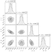 |
Fig. A.2. Differences between the recovered parameters, x′true = (a′,c′,b′,σ′intr)T and the true parameters, |
In summary, the transformation obtained from the best-fit A and b is a very accurate description of the bias induced by the flux limit in our simulated data. We use the inverse of this transformation, Eq. (A.3), in Sect. 5 to correct our inferred posterior density distribution from modelling the MUSE data.
All Tables
All Figures
|
Fig. 2. BPT-diagram (Baldwin et al. 1981) of the sources in our Hα λ6563-subsample for which we measure [N II] λ6584. All galaxies fall in the star-forming region of the diagram. The filled and open circles have S/N([N II] λ6584) > 3 and < 3, respectively, and the 5 sources encircled in red are detected in X-rays (Luo et al. 2016). The solid and dashed curve show the AGN boundary and maximum starburst line from Kauffmann et al. (2003) and Kewley et al. (2001), respectively. |
| In the text | |
|
Fig. 3. AGN diagnostics for the sources in our Hβ λ4861-subsample, including all sources which have S/N > 3 in the relevant emission lines. Overall, our sample is consistent with star-forming galaxies. We remove one X-ray detected AGN from the sample. Left: [O II] λ3727/Hβ vs. [O III] λ4959, 5007/Hβ diagnostic from Lamareille et al. (2004), solid line, with the uncertainty indicated by the dashed lines). Right: mass-excitation diagram from Juneau et al. (2011). Galaxies in the region between the dashed and solid lines are on average identified as intermediate between AGN and SF. |
| In the text | |
|
Fig. 1. Redshift distribution of our galaxies plotted against their (dust-corrected) SFR (1σ error bars are in grey). The colour denotes the stellar mass. The solid line depicts the lowest uncorrected SFR from Hβ λ4861 we can detect in the HUDF at each redshift (which is effectively determined by the requirement that S/N(Hγ λ4340)> 3; see Sect. 2.4). |
| In the text | |
|
Fig. 4. Histograms of the stellar mass distributions of the MUSE detected galaxies in the HUDF and the HDFS. The deep 30 h observations allow us to detect and subsequently infer a stellar mass and SFR for galaxies down to ∼107 M⊙. |
| In the text | |
|
Fig. 7. Left panel: sample of 179 star-forming galaxies observed with MUSE, plotted on the M*-SFR plane. The symbols indicate the field and colour indicates the redshift. The dashed lines show a constant sSFR, which is equivalent to a linear relationship: SFR ∝ M*. The red curve shows the model of the star formation sequence from Whitaker et al. (2014) for 0.5 < z < 1.0. The vertical grey dashed line indicates the selection for the low-mass fit (Sect. 5.2). Right panel: same as the left panel but with the data points removed, showing (the evolution of) the star formation sequence as seen by MUSE, according to Eq. (11). |
| In the text | |
|
Fig. 5. A comparison of the derived star formation rate (SFR) from the Hα λ6563, Hβ λ4861 and [O II] λ3727 luminosities for the HUDF (top panels, circles) and the HDFS (bottom panels, triangles). Left panels: logarithm of the SFR from Hα λ6563 vs. the difference between the log Hβ λ4861 and log Hα λ6563 SFRs. Right panels: same for Hβ λ4861 vs. [O II] λ3727. In each panel σ indicates the standard deviation (in dex) around the one-to-one relation. Colour indicates the signal-to-noise ratio (S/N) in the faintest line; Hγ λ4340. Only galaxies that allowed for more than one SFR indicator are included in the plot. Overall the SFRs from Hβ λ4861 and [O II] λ3727 agree reasonably well, considering we have not taken into account the metallicity dependence in SFR([O II] λ3727). The scatter in Hα λ6563 vs. Hβ λ4861 SFR is largely driven by Hγ λ4340 S/N. |
| In the text | |
|
Fig. 6. Optical depths at the wavelength of Hβ λ4861 as derived from both the Hβ λ4861/Hγ λ4340 and the Hα λ6563/Hβ λ4861-ratio, coloured by Hγ λ4340 signal-to-noise (S/N). The dashed line is the one-to-one relation. Overall the optical depths agree reasonably well, unless the Hγ S/N is low. Most galaxies actually show little dust (τ close to zero). The shaded area shows the regions of (unphysical) negative optical depth for each axis. We set the optical depth to zero for galaxies with negative τ as this is often consistent with the error bars and the offset is due to noise in the spectra. We note that some of the high-S/N outliers actually have discrepant Balmer ratios. If the inferred optical depth is very different, this will affect the comparison of the dust-corrected SFR from Hβ λ4861 and Hα λ6563 (see Fig. 5). |
| In the text | |
|
Fig. A.1. Results from the recovery experiment on mock galaxies. The points in the left and centre panels show one of the 30 realisations of 100 galaxies in (log M*, log(1 + z), log SFR)-space from a mock star formation sequence: logSFR ∝ alogM* + clog(1 + z), where in this particular case a = 0.8 and c = 2.0 with σintr = 0.5 dex. The colour indicates redshift, unless a mock galaxy falls below the solid line in the centre panel, indicating the flux limit of ∼3 × 10⁻¹⁹ erg s−1 cm−2, in which case it is a black point. The rightmost panels show the marginalised distributions (slope, redshift evolution, and intrinsic scatter) from combining all 30 realisations for this particular set of parameters. The thin and thick black lines indicate the results when taking into account all mock data and only the data above the flux limit, respectively, and are compared to the input values (dashed lines). With all data points (including noise), we can recover the input parameters sequence well. When applying the flux limit a slight bias towards a shallower slope and steeper redshift evolution appears. We plot all curves in the leftmost panel at the average redshift of the sample (z0). The red line is obtained after applying the correction to the fit of the data above the limit. These recovered curves are plotted in the leftmost panel as well and compared to the input mock relation. With our correction, we can recover the true input parameters well, even in the case of limited data. |
| In the text | |
|
Fig. 8. Projections of the 4D posterior distribution for the model parameters: slope (a), evolution (c), normalisation (b) and intrinsic scatter (σintr). The histograms on top show the marginalised distributions of the model parameters. The bias-corrected posterior median value and the 16th and 84th percentile are denoted by the dashed lines and by the values above the histograms. The contours show the 0.5, 1, 1.5 and 2σ levels. The posterior directly from the modelling is shown in black, red indicates the posterior after applying the bias correction (Eq. (A.3)). Figure created using the corner.py module (Foreman-Mackey 2016). |
| In the text | |
|
Fig. 9. The best-fit star formation sequence for the 179 star-forming galaxies observed with MUSE. The symbols indicate the dust-corrected tracer used to infer the SFR. The solid line shows best-fit relation, as presented in Eq. (11), and the dashed lines show the 1σ intrinsic scatter. We subtract the evolution from the y-axis and scale to the average redshift of the sample; z = 0.55. After accounting for evolution, the galaxies clearly follow the star formation sequence, down to the lowest masses and SFRs. The slightly larger fraction of galaxies that scatter into the high-mass, low-SFR regime may be a result of the flattening of the relation above M* = 1010 M⊙. |
| In the text | |
|
Fig. 10. A comparison of the slope (a) as a function of redshift (z) with studies from the literature that extend down to M* < 1010 M⊙ near our redshift range. Our best-fit (bias-corrected) slope from Eq. (11) is shown by the large star. As most studies have probed the slope in bins of redshift, we also include our results obtained using non-evolving redshift bins (Eqs. (14), (15) and (16); smaller blue stars). The literature results are from Renzini & Peng (2015), RP15),Kurczynski et al. (2016), K16), Bisigello et al. (2018), B18) and the low-mass (M* ≲ 1010 M⊙) power-law slopes from Whitaker et al. (2014), W14) and Lee et al. (2015), L15). We also add [SP14],Speagle2014 for reference, though it is inferred at higher masses. We indicate the field and SFR-tracer in brackets, though note that distinct calibrations for the same tracer may be used in different studies. In addition, we add the slopes predicted by (semi-)analytical models; Bouché et al. (2010), B10), Mitchell et al. (2014), M14), Mitra et al. (2015), Mi15), Cattaneo et al. (2017), C17), and hydrodynamical simulations; Sparre et al. (2015), Sp15), Furlong et al. (2015), F15), Sparre et al. (2017), Sp17). |
| In the text | |
|
Fig. A.2. Differences between the recovered parameters, x′true = (a′,c′,b′,σ′intr)T and the true parameters, |
| In the text | |
Current usage metrics show cumulative count of Article Views (full-text article views including HTML views, PDF and ePub downloads, according to the available data) and Abstracts Views on Vision4Press platform.
Data correspond to usage on the plateform after 2015. The current usage metrics is available 48-96 hours after online publication and is updated daily on week days.
Initial download of the metrics may take a while.