| Issue |
A&A
Volume 618, October 2018
|
|
|---|---|---|
| Article Number | A96 | |
| Number of page(s) | 9 | |
| Section | The Sun | |
| DOI | https://doi.org/10.1051/0004-6361/201833561 | |
| Published online | 22 October 2018 | |
Solar energetic particles and galactic cosmic rays over millions of years as inferred from data on cosmogenic 26Al in lunar samples
1
Space Climate Research Unit, University of Oulu, Finland
e-mail: This email address is being protected from spambots. You need JavaScript enabled to view it.
2
Sodankylä Geophysical Observatory, University of Oulu, Finland
3
Ioffe Physical-Technical Institute, 194021 St. Petersburg, Russia
Received:
4
June
2017
Accepted:
10
July
2018
Abstract
Aims. Lunar soil and rocks are not protected by a magnetic field or an atmosphere and are continuously irradiated by energetic particles that can produce cosmogenic radioisotopes directly inside rocks at different depths depending on the particle’s energy. This allows the mean fluxes of solar and galactic cosmic rays to be assessed on the very long timescales of millions of years.
Methods. Here we show that lunar rocks can serve as a very good particle integral spectrometer in the energy range 20–80 MeV. We have developed a new method based on precise modeling, that is applied to measurements of 26Al (half-life ≈0.7 megayears) in lunar samples from the Apollo mission, and present the first direct reconstruction (i.e., without any a priori assumptions) of the mean energy spectrum of solar and galactic energetic particles over a million of years.
Results. We show that the reconstructed spectrum of solar energetic particles is totally consistent with that over the last decades, despite the very different levels of solar modulation of galactic cosmic rays (ϕ = 496 ± 40 MV over a million years versus (ϕ = 660 ± 20 MV for the modern epoch). We also estimated the occurrence probability of extreme solar events and argue that no events with the F(>30 MeV) fluence exceeding 5×10¹⁰ and 1011 cm−2 are expected on timescales of a thousand and million years, respectively.
Conclusions. We conclude that the mean flux of solar energetic particles hardly depends on the level of solar activity, in contrast to the solar modulation of galactic cosmic rays. This puts new observational constraints on solar physics and becomes important for assessing radiation hazards for the planned space missions.
Key words: Sun: particle emission / Sun: activity / Moon
© ESO 2018
1. Introduction
Solar energetic particles (SEPs), which form an essential component of the radiation environment near Earth (Vainio et al. 2009; Schwadron et al. 2017), appear as sporadic fluxes of energetic protons and a small fraction of heavier particles associated with powerful solar flares and/or coronal mass ejections. Knowledge of the mean SEP flux in the energy range of several tens of MeV, as well as an assessment of the strength of occurrence probability of extreme SEP events are crucially important for the modern space-based technological society (e.g., NCRP 2006). One of the most important parameters of the near-Earth radiation environment is the integral flux of energetic particles with energy above 30 MeV, F(>30 MeV) (e.g., Shea & Smart 1990; Feynman et al. 1993). Direct space-borne measurements of SEPs over the last decades suggest that the average SEP flux is dominated by rare major events (Bazilevskaya et al. 2014) and varies between individual solar cycles by an order of magnitude (Reedy 2012). However, the direct data were obtained during the period of unusually high solar activity known as the modern grand maximum (MGM, see Solanki et al. 2004). Therefore, it is unclear whether the modern data are representative for longer timescales.
Extreme SEP events in the past can be studied by means of cosmogenic isotopes (primarily 14C and 10Be) in terrestrial natural archives (e.g., Miyake et al. 2012; Güttler et al. 2015; Usoskin 2017) on a timescale of up to 10 000 years; however, because of atmospheric and magnetospheric shielding, they cannot provide information about solar particles with the energy of tens of MeV (Kovaltsov et al. 2014) that is most important for technological impacts. Ideally, this ought to be studied using data from the space outside the Earth’s atmosphere and magnetosphere, such as meteorites (e.g., Mancuso et al. 2018) or lunar samples. The lunar surface is not shielded from incoming radiation and keeps the information about its flux in the past. Cosmogenic isotopes are produced in situ in lunar rocks, allowing us to reconstruct the mean energy spectrum of energetic particles, although without temporal resolution. This idea was explored earlier (Reedy & Arnold 1972), when the SEP flux was estimated using measurements of lunar rocks brought to Earth by the Apollo missions. However, the earlier efforts (e.g., Rao et al. 1994; Fink et al. 1998; Jull et al. 1998; Nishiizumi et al. 2009) were model-dependent. In fact, those works did not provide true reconstructions of the spectrum, but only estimated the parameters of an explicitly prescribed functional shape (exponential over rigidity; see Eq. (4)). Here we demonstrate that a lunar rock with cosmogenic 26Al produced in situ can serve as an integral particle spectrometer able to reconstruct the SEP energy spectrum over long-term scales directly from measurements without any a priori assumptions on the spectral shape.
2. Data and methods
2.1. Parameters of the used lunar samples
Here we use data of 26Al (half-life 717 000 years) activity in two lunar samples, 64 455 and 74 275, brought by Apollo missions 16 and 17, and subsequently measured in different laboratories.
Sample 64 455 is an egg-shaped object of about 5 cm long and 3 cm across collected directly from the lunar surface. Full information on its physical and chemical parameters is available elsewhere1 (Meyer 2011). The content of 26Al was measured by Nishiizumi et al. (2009). The sample was modeled using hemispherically concentric shells (R = 7 g cm−2) lying upon a flat lunar-soil surface. The irradiation age and erosion rate were estimated as 2 Myr and 0–0.5 mm Myr−1, respectively (Meyer 2011).
Sample 74 275 is a flat knob-shaped object, 17 cm long, 12 cm across, and 4 cm thick, collected from the lunar surface. Full information is available elsewhere2 (Meyer 2011). It was measured by Fink et al. (1998) and modeled using “knob” geometry (R = 78 g cm−2) and columnar-averaged isotope activity, as lying upon a flat lunar-soil surface. The irradiation age and erosion rate were estimated as 2.8 Myr and 1–2 mm Myr−1, respectively (Meyer 2011).
We also use 26Al measurements (Rancitelli et al. 1975; Nishiizumi et al. 1984) in the 242-cm long Apollo 15 deep-drill core, which was modeled using the slab geometry and chemical composition according to Gold et al. (1977). More detailed information is available3 at (Meyer 2011).
2.2. Model of 26Al production
Production of an isotope by cosmic rays inside matter is numerically modeled using the concept of the yield function. The isotope’s production rate Q(h) at depth h in a sample is related to the flux of primary energetic particles, SEPs or galactic cosmic rays (GCRs), as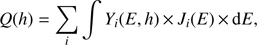 (1)where index i denotes the type of primary energetic particles, i.e., protons, α-particles, or heavier species; Yi(E,h) is the isotope yield function; and Ji(E) is the differential intensity of particles with energy E. The intensity J is typically used to quantify GCRs in units of [cm2 s sr MeV]−1, while for SEPs the omnidirectional flux F [cm2 s MeV]−1 is often used, which is related to the intensity, in the isotropic case, as F(E) = 4π × J(E) (see, e.g., chapter 1.6 of Grieder 2001).
The yield function is calculated as (2)where k is the index of primary or secondary particles (protons, neutrons, α-particles, pions), Sk(E′) is the efficiency of the isotope production by a particle of type k with energy E′, Nk,i(E,E′,h) is the concentration at depth h of primary and secondary particles of type k with energy E′ corresponding to the primary particle of type i with energy E, and vk(E′) is the particle’s velocity. Nk,i(E,E′,h) is a result of numerical simulations of the particle transport in lunar matter and is calculated per unit intensity (Ji = 1 cm−2 s−1 sr−1) of monoenergetic primary particles. The efficiency of isotope production by particles of type k is
 (3)where j indicates the type of target nuclei in a lunar sample, Cj is their content in one gram of matter, and σj,k(E′) is the cross section of the corresponding nuclear reactions. The efficiency S depends on the chemical composition of a sample and needs to be calculated for each case individually. The cross sections of 26Al production by protons were adopted from Nishiizumi et al. (2009) and Reedy (2007), while those for α-particles were taken according to Tatischeff et al. (2006). The cross sections for 26Al production by neutrons on Al and Si were taken from Reedy (2013) and assumed to be identical to those for the proton reactions for other nuclei (Ca, Ti, Fe). We also considered the 26Al production by charged pions, whose contribution was typically neglected earlier but is shown to be essential in dense matter (Li et al. 2017). The corresponding cross sections were extracted from the Geant4 model (Agostinelli et al. 2003). An example of the efficiency of 26Al production for proton reactions in a lunar rock is shown in Fig. 1. We can see that three elements (Mg, Al, and Si) dominate the production in different energy ranges. The isotope 26Al enables the most accurate reconstruction of the SEP spectrum due to the low energy threshold and high efficiency of its production by low-energy particles (Fig. 1A), in contrast to other isotopes 10Be, 14C, and 36Cl, also measured in lunar rocks but having higher energy thresholds, lower efficiency (Fig. 1B), and accordingly lower sensitivity to SEPs versus GCRs, even in the upper layers (Fink et al. 1998; Jull et al. 1998; Nishiizumi et al. 2009).
 |
Fig. 1. Efficiency of production (see Eq. 3) of cosmogenic isotopes by primary and secondary protons of energy E in the lunar sample 64 555, as computed here. Panel A: production of 26Al : contributions from different target nuclei are denoted by dashed lines, while the thick red curve is the total sum. Panel B: summary productions of different long-lived cosmogenic isotopes, as denoted in the legend. The red curve is identical to that in panel A. |
Specific yield functions were calculated individually for each particular case considered here (two lunar rocks and the deep core; see Sect. 2.1). Primary particles were assumed to arrive isotropically from the upper hemisphere. Their composition was considered to be only protons for SEPs, and protons and heavier species for GCRs. An example of the yield function for 26Al at different depths is shown in Fig. 2.
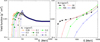 |
Fig. 2. Examples of the yield function of 26Al production in the lunar rock for different depths as denoted in the legend in units of cm2/g. Panel A corresponds to shallow layers of sample 64 455 in idealized conditions (infinite exposition age, no erosion). Panel B corresponds to the Apollo 15 long drill core. These yield functions are shown here for illustration, but for each case they were computed individually considering realistic exposition age, erosion rate, geometry, chemical composition, and measurement details (see Sect. 2.1). |
Computations of the isotope production in the deep-drill core require simulations of the nucleonic cascade initiated by energetic particles deeper in matter. This was made by full Monte Carlo simulations, using the Geant4 toolkit (version 4.10 Agostinelli et al. 2003) for nuclear interactions of primary and secondary particles in the core and applying the slab geometry. The chemical composition of the Apollo 15 deep-drill core was taken according to (Gold et al. 1977).
It was proposed earlier (Reedy & Arnold 1972) that SEP related production in lunar rocks can be modeled analytically since SEP energy is insufficient to initiate a nucleonic cascade. We have checked this assumption (Poluianov et al. 2015) and found that it works reasonably well for the upper layers shallower than 5–7 g cm−2. Accordingly, we simulated 26Al production by SEP protons in the shallow layers by direct integration of the analytical formulas for the exact geometry in each case. Samples were considered to be lying on typical lunar soil with a flat surface and the chemical composition of the Apollo 15 deep-drill core.
2.3. Lunar rock as an integral spectrometer
The yield function for 26Al produced in lunar rocks by protons at shallow depths (<7 g cm−2, Fig. 2A) is step-like with the sharp energy threshold growing with depth, where 26Al is produced directly by impinging energetic particles as a result of spallation of target nuclei Mg, Si, and Al (Fig. 1A) without development of a nuclear cascade. Spallation reactions define the primary particle’s energy threshold, which increases with depth because of ionization losses. This yield-function shape is close to that of an ideal integral particle spectrometer, which is a detector whose response is directly proportional to the integral flux of primary particles with energy above a threshold E*, with the yield-function being step-like, i.e., zero for energy below E*, and a constant value for E ≥ E*.
2.3.1. SEP spectral shape
Here we show that production of 26Al in the upper layer of a lunar rock is indeed a good integral spectrometer for protons of SEP energies. This allows the SEP spectrum to be reconstructed directly from the measured data, without any a priori assumption on its exact spectral shape. To check this and to assess the related uncertainties, we considered two spectral shapes often used in earlier SEP studies: an exponent over rigidity (EXP; Freier & Webber 1963) (4)and a power law (POW) over energy (Van Hollebeke et al. 1975)
 (5)Overall, POW tends to provide a spectrum that is too hard with an excess of high- and low-energy particles, while EXP yields a softer (at the high-energy tail) spectrum with an excess of mid-energy particles. These two models bound more realistic cases, such as the modified power law (Crampet al. 1997), i.e., a power law with a gradually increasing spectral index; the Ellison–Ramaty spectrum (Ellison & Ramaty 1985), a power law with an exponential roll-off at higher energies; Band-function (Band et al. 1993; Raukunen et al. 2018), a double power law, hard at low energies and soft at higher energies with a smooth junction; or Weibull representations (Pallocchia et al. 2017) of the SEP energy spectrum. An agreement between the results based on the POW and EXP models would imply that the method is model-independent, while the difference between them can serve as a conservative measure of the model uncertainty.
2.3.2. Effective energy of isotope production
Here we define the effective energy E* of the isotope production (see Kovaltsov et al. 2014) as the energy for which the scaling ratio K = F(>E*)/A is approximately constant in a wide range of spectral parameters. Here F(>E) is the integral omnidirectional flux of protons with energy above E; the activity A of the radioisotope (quantified via the disintegration rate per minute per kilogram, dpm kg−1) at a given depth h is computed from the production rate Q (Eq. (1)), assuming a flux of particles constant in time and explicitly considering the exact composition, exposure age T, and erosion rate r for each sample as (6)where h′ = h + ρrt is the depth at time t with account of erosion, ρ is the rock’s density, and τ is the lifetime of the isotope. We assumed in computations that the production rate Q and erosion rate r are constant in time. An example is shown in Fig. 3 (panels A and B) for the EXP and POW models (see Eqs. (4) and (5), respectively) for the depth h = 1 g cm−2. We can see that there is a value of E* at which K is roughly constant in a wide parametric range. As the range of parameters, we considered R0 = [30 − 200] MV for the EXP model and γ = [2–5] for the POW model, which roughly covers the range of values for the observed SEP events during the last decades. We have checked that the exact choice of the parametric range does not affect the results. The exact values of E* were found by minimizing the relative variability ΔK/K, where ΔK = Kmax − Kmin is the full range of the K-values within the studied interval of spectral parameters. For the examples shown in Figs. 3A and B, the values of E* were found to be 39.6 MeV and 39.1 MeV, respectively, for the EXP and POW models, with the corresponding ΔK/K ≤ 2% in both cases.
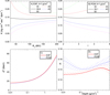 |
Fig. 3. Panel A: dependence of the scaling factor K on the characteristic rigidity R 0 of the EXP model for the depth of 1 g cm−2 for different values of the effective energy E*, as denoted in the legend (in MeV). Panel B: same as A, but for the POW model with the index γ. Panel C: effective energy E* as a function of depth in lunar sample 64 455 for the EXP and POW models. Panel D: same as C, but for the best-fit scaling factor K; the hatched areas represent the full-range ΔK-values. |
The resulting “calibration” curve of E* as a function of depth h is shown in panel C for the two spectral models. We can see that the two curves nearly coincide in the range of depths from 0.1 to 3 g cm−2, giving a clear relation to the effective energy within ≈20–60 MeV. We neglected the uncertainties of the definition of E* in each case, but instead took the difference between the EXP and POW models (ΔE*), which is less than 1 MeV. The corresponding scaling factor K is shown in panel D for the two models with the ΔK-uncertainties indicated. We can see that the EXP and POW models agree with each other within the uncertainties in the depth range 0.1–5 g cm−2 (E* = [20–80] MeV), but diverge at shallower and deeper depths. Therefore, there is a nearly one-to-one relation between the depth in the sample and energy E* of the SEP particles; the measured isotope activity at this depth A(h) can then be directly translated into the integral flux F(>E*) via the coefficient K.
Thus, the method is suitable for a robust and model-independent reconstruction of the particle spectrum in the energy range between 20 and 80 MeV. This provides a straightforward way to reconstruct the SEP spectrum directly from the measured depth profile of 26Al activity in the upper layers of lunar samples.
2.4. Estimation of uncertainties
We considered several sources of uncertainties:
Measurements. Measurement errors of the isotope activity A are converted into production rate Q using the sample’s age and erosion rate. The ensuing errors of Q are called σQ. These errors are treated as distributed normally around Q with the corresponding standard deviation. In addition, there is the error of the GCR fitting σGCR (see Sect. 3.1), which is also considered as normally distributed.
Model. The model uncertainty is related to the definition of the effective energy E* and the conversion coefficient K for the given depth in a sample (see Sect. 2.3). These uncertainties are treated as uniformly distributed within the full-range interval.
SEP spectral shape. Model computations were made for two bounding spectral shapes: exponential EXP and power-law POW (Eqs. (4) and (5) in Sect. 2.3). These two models were considered to have equal probabilities.
Erosion rate. The erosion rate for each sample remains an unknown parameter, with the range estimated as 0–0.5 and 1–2 mm Myr−1 for samples 64 555 and 74 275, respectively (see Table 2). These uncertainties enter conversion of the measured isotopes activities A into the production rates.
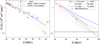 |
Fig. 4. Integral omnidirectional fluxes F(>E) of solar energetic protons with energy above the given value E. Panel A: reconstruction of the million-year spectrum based on 26Al in lunar samples. The red and blue dots depict reconstructions (see Table 1) from measurements of 26Al in lunar samples 64 455 (erosion rate, r = 0 and 0.5 mm Myr−1) and 74 275 (erosion rate r = 1 and 2 mm Myr−1), respectively, as denoted in the legend. The thick line and the hatched area depict the average and the full-range uncertainties of the reconstructed fluxes for the two samples, considering all the uncertainties, including those of the erosion rate and of the spectral shape. Exact values are given in Table 2. Panel B: comparison with other spectra. The thick gray line with hatched area is the present reconstruction (identical to that in panel A). Colored lines depict earlier estimates of the SEP spectra, explicitly assuming the EXP shape (Eq. (4)), from 26Al by (Fink et al. 1998, Fi98), from 14C by (Jull et al. 1998, denoted Ju98) and from 26Al and 36Cl by (Nishiizumi et al. 2009, Ni09). The orange stars depict the mean values of F(>30 MeV) and F(>60 MeV) for the last solar cycles 1954–2008 (Reedy 2012), error bars being the standard error of the mean over individual cycles. The thick black line depicts the GCR contribution (ϕ = 496 MV). |
Uncertainties of the final result were assessed using a Monte Carlo method as described below. For each data point for a given sample and depth h we made 106 realizations of the reconstructed SEP flux F(>E*). For each realization we first took a normally distributed random number with the mean Q(h) and standard deviation of σQ(h). Then the value of the GCR related background was taken in a similar random way using the estimate of σGCR. Thus, the value of QSEP(h) was obtained. Next, we randomly chose the model between exponential and power law, and computed the energy E* (from Fig. 3C) taking the scaling factor K as a uniformly distributed random number from the interval K ± ΔK (from Fig. 3D). From these obtained 106 values we computed the mean flux 〈F〉 and the uncertainties defined as the full range of E* and the upper and lower 16th percentiles of the F distribution. The final result is shown in Fig. 4 and listed in Table 2. The gray-shaded area in Fig. 4 denotes the full range of the reconstructed spectrum, which is an envelope of individual reconstructions.
3. Results
3.1. Galactic cosmic rays on the mega-year timescale
Since lunar rocks are bombarded by both SEPs and GCRs, we need first to remove the contribution of GCRs into the isotope production before reconstructing SEPs. GCRs are much more energetic, but less abundant in the lower energy range than SEPs. They penetrate much deeper into matter, where initiate nucleonic cascades and dominate the isotope production at depths >20 g cm−2.
We adopted a general description of the GCR spectral shape in the form of a force-field approximation (Gleeson & Axford 1968; Caballero-Lopez & Moraal 2004), which is a common and well validated way to describe the long-term variability of GCRs (Usoskin et al. 2005; Herbst et al. 2010). The near-Earth energy spectrum Ji(E), of GCR particles of type i (proton or heavier species), characterized by the charge Zi and mass Ai numbers, can be presented via the unmodulated local interstellar spectrum (LIS) JLIS,i and the so-called modulation potential ϕ as  (7)where E is the particle’s kinetic energy per nucleon, ΦI = ϕ(eZi/Ai), and Er = 0.938 GeV/nucleon is the rest mass of a proton. The energy spectrum of GCR is defined by a single parameter, the modulation potential ϕ, which quantifies modulation of GCR inside the heliosphere by solar magnetic activity. The reference local interstellar spectrum (LIS) of protons was taken in the form provided by Vos & Potgieter (2015) considering direct in situ measurements of low-energy GCR beyond the termination shock and near-Earth measurements in high-energy range. Results, based on other LIS models, can be straightforwardly converted (Asvestari et al. 2017). The nucleonic fraction of helium and heavier nuclei was standardly considered as 0.3 to protons in LIS (e.g., Usoskin et al. 2011). We assumed that LIS is constant on a million-year timescale. Figure 5 shows dependence of the 26Al production by GCR in the deep drill core as a function of the depth h and the modulation potential ϕ. Applying this dependence, we fitted the measured concentrations of 26Al in the Apollo 15 deep core (Nishiizumi et al. 1984; Rancitelli et al. 1975) to find the best-fit values of the modulation potential (Fig. 6). The fit was performed by minimizing χ2 as shown in panel B. The best-fit value of the modulation potential was found to be ϕ = 496 ± 40 MV for the last million years, which is considered hereafter.
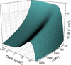 |
Fig. 5. Modeled production Q of cosmogenic 26Al by galactic cosmic rays in a lunar soil as a function of the modulation potential ϕ and depth h. The production was computed for the slab geometry and the chemical composition of the Apollo 15 deep drill core (Gold et al. 1977). |
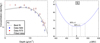 |
Fig. 6. Determination of the mean GCR level. Panel A: measured (N84; Nishiizumi et al. 1984) and red (R75; Rancitelli et al. 1975) dots) and the best-fit GCR-induced activity of 26Al in the Apollo 15 deep drill core. Datapoints used for the fit are in black circles. Since activity at depths shallower than 20 g cm−2 can be affected by SEPs, shallow points were not used in the fit. The gray hatched area denotes the 68% confidence interval defined in panel B. Panel B: χ2 statistics for the fit of the modeled 26Al activity shown in Panel A as a function of the modulation potential ϕ. The best-fit
|


This value is significantly smaller than the mean modulation potential ϕ = 666 ± 20 MV for the period 1951–2016 (Usoskin et al. 2017), but consistent within uncertainties with the mean modulation over the Holocene (Usoskin et al. 2016) ϕ = 449 ± 70 MV (reduced to the same LIS). This highlights the fact that the second half of the 20th century was characterized by MGM with unusually high solar activity.
3.2. Mean SEP spectrum estimate
The corresponding GCR contribution was subtracted from the measured isotope content, and the remaining activity was ascribed to SEP, whose spectrum was further reconstructed using the “calibration” curves shown in Fig. 3C and D. The final reconstruction of the SEP spectrum is shown in Fig. 4A for the two lunar samples and for a range of erosion rates. Uncertainties were calculated as described in Sect. 2.4. The full range uncertainty (the envelope over different samples and erosion rates) is shown by the gray hatched area. The reconstructed fluxes lie very close to each other in the energy range of 20–35 MeV, being almost independent on the exact sample, spectral shape, and erosion rate, with the full-range relative uncertainty (including the model uncertainty) being within 20%. This energy range corresponds to the F(>30 MeV), which is often considered as the radiation environment. Thus, the F(>30 MeV) flux is quite robustly defined here. The uncertainty grows with energy, reaching 40% at 60 MeV and a factor of two at 80 MeV. The summary spectrum, which includes the mean and the full-range uncertainties (gray area in Fig. 4), is given in Table 2 and serves as our final estimate of the mean SEP spectrum over million of years.
As a consistency check, we performed the following computation: from the spectra reconstructed above (both GCR and SEP) we calculated, using realistic geometry and chemical compositions, the expected activity of 26Al in a lunar rock and compared it with the actual measurements (Fig. 7).
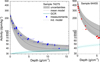 |
Fig. 7. Comparison of the measured 26Al activity in the analyzed samples 74 274 (blue points in panel A, from Fink et al. 1998) and 64 455 (red points in panel B, from Nishiizumi et al. 2009) with the values computed here using the final reconstructed spectrum (Table 2 in the main text) as shown by the solid black line (the mean activity) with the full-range uncertainty (gray area). The dashed curves with the hatched areas correspond to spectra reconstructed for individual samples (Table 1). The light blue hatched area with the olive curve depicts the GCR contribution to the activity. |
A comparison of the new reconstructed million-year SEP spectrum with earlier estimates and the direct space-era data is shown in Fig. 4B. Color curves present earlier estimates of the SEP spectrum (Fink et al. 1998; Jull et al. 1998; Nishiizumi et al. 2009) explicitly assuming its EXP shape (Eq. (4)). They all agree within a factor of two and fit into the uncertainty of the present reconstruction (except for the 26Al -based Ni09). The curves are shown in the energy range corresponding to the production threshold (see Fig. 1B), since their extension to the lower energy range would be based on an extrapolation of the exponential shape but not on data. The SEP spectrum is more uncertain for energies above 100 MeV, where the contribution of GCR becomes dominant. We conclude that the present direct reconstruction of the mean SEP spectrum is consistent with earlier estimates which were obtained using an explicit a priori assumption on the EXP shape.
For comparison, we also show the mean integral fluxes F(>30 MeV) and F(>60 MeV) for the last solar cycles 1954–2008 (Reedy 2012) as orange stars. The flux reconstructed for the last million years agrees, within the uncertainties, with that for the last cycles. This is an interesting result since solar activity (the modulation potential ϕ) was significantly higher during the recent decades due to the Modern grand maximum than in the past (Sect. 3.1). This implies that the mean SEP flux does not depict a notable dependence on the overall solar activity level. This result is concordant with the fact that strongest known extreme SEP events (Miyake et al. 2012, 2013; Usoskin et al. 2013; Jull et al. 2014; Wang et al. 2017), such as the events of 775 AD, 993 AD, BC 3372, and the Carrington event of 1859, occurred during periods of moderate solar activity. This provides new observational constraints Hudson 2010.
3.3. Estimate of the SEP event occurrence probability
Following the idea presented by Kovaltsov & Usoskin (2014), we can assess the occurrence probability density function (OPDF) of SEP events, based on the reconstructed spectrum. Since only the mean flux of SEP can be directly estimated from lunar data, further modeling is needed to assess the occurrence rate of individual events. For example, the entire mean flux can be produced by a huge single event that occurred a while ago. Such an extreme assumption was made, for example, by Reedy (1996), but it is obviously unrealistic since it assumes that there are no other weaker events during the lifetime of the isotope. In reality, there is always a distribution of events over their strength and occurrence rate. A more appropriate estimate can be made by assuming such a realistic distribution.
Let us assume that OPDF of SEP annual fluence can be approximated by the Weibull distribution (Weibull 1951), which is often used to describe the occurrence probability of solar events (see, e.g., Gopalswamy 2018, and discussion therein)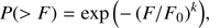 (8) where P is the probability that a SEP event with the fluence greater than F will occur within one year, and k and F0 are two fitted parameters of the model. Then the mean fluence 〈F〉 is defined as
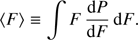 (9)Now this model can be fitted to data using several observational constraints:
-
The mean F(>30 MeV) flux (Eq. (9)) takes the values between 1 and 1.4 × 10⁹ (cm2 yr)−1 as corresponding to the mean reconstructed values (Table 2);
-
The fact that no events with F(>30 MeV) exceeding 1011 (cm2 yr)−1 have been found and are unlikely to be found over the Holocene (Usoskin 2017) poses an upper limit of the corresponding OPDF as P(>1011 cm−2) ≤ 2.1 × 10⁻⁴ yr−1;
-
A lower limit of P(>1010 cm−2) ≥ 2.8 × 10⁻⁴ yr−1 is set that corresponds to the three historical events of 3372 BC (Wang et al. 2017), 775AD (Miyake et al. 2012), and 994AD (Miyake et al. 2013) securely found during the Holocene, but there may be more similar events discovered (e.g., Park et al. 2017) since the entire record has not been analyzed yet (Usoskin 2017).
The suitable parameter range was found as F0 = [0.2 − 0.8] 109 cm−2 yr−1 and k = [0.3 − 0.57] with a high correlation between them. The corresponding distribution function is shown as the red hatched area in Fig. 8 and describes well all the data points including the data from lunar rocks. It is interesting to note that the first blue dot in Fig. 8 lies too low versus the reconstructed OPDF, implying that the number of known events with F(>30 MeV) ≥ 2 × 10¹⁰ (cm2 yr)−1 is smaller than expected and that we expect more events of this strength to be discovered over the Holocene (Park et al. 2017). According to this estimate, no events with F(>30 MeV) ≥ 5 × 10¹⁰ and ≈1011 protons cm−2 are expected on timescales of a thousand and a million years, respectively.
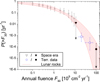 |
Fig. 8. Occurrence probability density function (OPDF) of solar energetic particles with the annual F(>30 MeV) fluence exceeding the giving value. The triangles denote OPDF based on the data for the space era (Usoskin & Kovaltsov 2012). The circles correspond to the SEP events estimated from the terrestrial cosmogenic isotope data (modified after Usoskin 2017). Open symbols indicate the measured/estimated values, filled symbols indicate a conservative upper bound. Error bars bound the 68% confidence interval. The red hatched area encompasses the OPDF estimated in this work from 26Al in lunar samples. |
4. Discussion and conclusions
We have shown that activity of 26Al measured in the upper shallow layers (<5 g cm−2) of lunar rocks serves as a good integral particle spectrometer in the energy range of 20–80 MeV. The lower bound is limited by the threshold of the isotope’s production reactions. On the other hand, more energetic particles with energy above 100 MeV can initiate nucleonic cascades in deeper layers making the yield function of the isotope’s production increase with energy (Fig. 2B), which distorts the characteristics of an integral spectrometer. Moreover, the GCR contribution to the isotope production grows with depth (Fig. 4), which makes separation of the SEP signal less robust in deeper layers. Thus, only the SEP flux in the energy range 20–80 MeV can be reliably reconstructed.
Although the idea of reconstruction of the spectrum of solar energetic particles from lunar samples has been exploited in the past, a new approach based on precise computations of the yield function makes it possible to use lunar rocks as a good particle spectrometer able to estimate the SEP spectrum without any a priori assumptions on its shape. Using this method, we provided the first realistic model-independent reconstruction of the SEP energy spectrum in the energy range 20–80 MeV on a timescale of a million years and showed that it is consistent with earlier estimates and with the modern values. We also evaluated, using the 26Al data from deep layers, the million-year mean flux of GCR, which appears to be significantly less modulated (the modulation potential ϕ = 496 ± 40 MV) than during the last decades (ϕ = 660 ± 20 MV), confirming the importance of MGM of solar activity in the second half of the twentieth century. The fact that the mean million-year SEP spectrum is consistent with the modern values, obtained during the MGM, implies a lack of notable dependence of the SEP flux on the level of solar activity, consistent with the fact that the strongest known historical solar event occurred during periods of moderate solar activity. This puts new observational constraints on solar physics and becomes crucially important for assessing radiation hazards for the planned space missions.
Acknowledgments
This work was supported by the Center of Excellence ReSoLVE (Project 272157) of the Academy of Finland. The authors are thankful to Anton Artamonov for the help in verification of the Geant4 model of lunar samples.
References
- Agostinelli, S., et al. (GEANT4 Collaboration) 2003, Nucl. Inst. Meth. Phys. Res. A, 506, 250 [NASA ADS] [CrossRef] [Google Scholar]
- Asvestari, E.,Gil, A.,Kovaltsov, G. A., &Usoskin, I. G. 2017, J. Geophys. Res. (Space Phys.), 122, 9790 [Google Scholar]
- Band, D.,Matteson, J.,Ford, L., et al. 1993, ApJ, 413, 281 [NASA ADS] [CrossRef] [Google Scholar]
- Bazilevskaya, G. A.,Cliver, E. W.,Kovaltsov, G. A., et al. 2014, Space Sci. Rev., 186, 409 [NASA ADS] [CrossRef] [Google Scholar]
- Caballero-Lopez, R., &Moraal, H. 2004, J. Geophys. Res., 109, A01101 [Google Scholar]
- Cramp, J. L.,Duldig, M. L.,Flückiger, E. O., et al. 1997, J. Geophys. Res., 102, 24237 [Google Scholar]
- Ellison, D. C., &Ramaty, R. 1985, ApJ, 298, 400 [Google Scholar]
- Feynman, J.,Spitale, G.,Wang, J., &Gabriel, S. 1993, J. Geophys. Res., 98, 13 [Google Scholar]
- Fink, D.,Klein, J.,Middleton, R., et al. 1998, Geochim. Cosmochim. Acta, 62, 2389 [NASA ADS] [CrossRef] [Google Scholar]
- Freier, P. S., &Webber, W. R. 1963, J. Geophys. Res., 68, 1605 [NASA ADS] [CrossRef] [Google Scholar]
- Gleeson, L., &Axford, W. 1968, ApJ, 154, 1011 [NASA ADS] [CrossRef] [Google Scholar]
- Gold, T.,Bilson, E.,Baron, R. L.,Ali, M. Z., &Ehmann, W. D. 1977, Chemical and optical properties at the Apollo 15 and 16 sites, ed. R. B. Merril, Lunar Planet (Conf. Proc.: Sci). [Google Scholar]
- Gopalswamy, N. 2018, in Chapter 2 - Extreme Solar Eruptions and their Space Weather Consequences, ed. N. Buzulukova (Elsevier), Extreme Events in Geospace, 37 [Google Scholar]
- Grieder, P. 2001, in Cosmic Rays at Earth (Amsterdam: Elsevier Science) [Google Scholar]
- Güttler, D., Adolphi, F.,Beer, J., et al. 2015, Earth Planet. Sci. Lett., 411, 290 [NASA ADS] [CrossRef] [Google Scholar]
- Herbst, K.,Kopp, A.,Heber, B., et al. 2010, J. Geophys. Res., 115, D00120 [CrossRef] [Google Scholar]
- Hudson, H. S. 2010, Nat. Phys., 6, 637 [NASA ADS] [CrossRef] [Google Scholar]
- Jull, A.,Cloudt, S.,Donahue, D., et al. 1998, Geochim. Cosmochim. Acta, 62, 3025 [NASA ADS] [CrossRef] [Google Scholar]
- Jull, A.,Panyushkina, I.,Lange, T., et al. 2014, Geophys. Res. Lett., 41, 3004 [Google Scholar]
- Kovaltsov, G. A., &Usoskin, I. G. 2014, Sol. Phys., 289, 211 [NASA ADS] [CrossRef] [Google Scholar]
- Kovaltsov, G. A.,Usoskin, I. G.,Cliver, E. W.,Dietrich, W. F., &Tylka, A. J. 2014, Sol. Phys., 289, 4691 [Google Scholar]
- Li, Y.,Zhang, X.,Dong, W., et al. 2017, J. Geophys. Res. (Space Phys.), 122, 1473 [NASA ADS] [Google Scholar]
- Mancuso, S.,Taricco, C.,Colombetti, P., et al. 2018, A&A, 610, A28 [NASA ADS] [CrossRef] [EDP Sciences] [Google Scholar]
- Meyer, C. 2011, Lunar Sample Compendium. Technical Report. NASA. USA. Available at, https://curator.jsc.nasa.gov/lunar/lsc/index.cfm [Google Scholar]
- Miyake, F.,Nagaya, K.,Masuda, K., &Nakamura, T. 2012, Nature, 486, 240 [NASA ADS] [CrossRef] [Google Scholar]
- Miyake, F.,Masuda, K., &Nakamura, T. 2013, Nat. Comm. 4, 1748 [Google Scholar]
- NCRP, 2006, Information Needed to Make Radiation Protection Recommendations for Space Missions Beyond Low-earth Orbit. NCRP report, National Council on Radiation Protection and Measurements, https://www.ncrppublications.org/Reports/153 [Google Scholar]
- Nishiizumi, K.,Arnold, J. R.,Klein, J., &Middleton, R. 1984, Earth Planet. Sci. Lett., 70, 164 [NASA ADS] [CrossRef] [Google Scholar]
- Nishiizumi, K.,Arnold, J. R.,Kohl, C. P., et al. 2009, Geochim. Cosmochim. Acta, 73, 2163 [NASA ADS] [CrossRef] [Google Scholar]
- Pallocchia, G.,Laurenza, M., &Consolini, G. 2017, ApJ, 837, 158 [NASA ADS] [CrossRef] [Google Scholar]
- Park, J.,Southon, J.,Fahrni, S.,Creasman, P. P., &Mewaldt, R. 2017, Radiocarbon, 59, 1147 [CrossRef] [Google Scholar]
- Poluianov, S.,Artamonov, A.,Kovaltsov, G., &Usoskin, I. 2015, in Flux of Solar Energetic Particles in the Distant Past: Data from Lunar Rocks, A. S. Borisov, V. G. Denisova, &Z. M. Guseva, eds. 34th International Cosmic Ray Conference (ICRC2015), 51 [Google Scholar]
- Rancitelli, L. A., Fruchter, J. S.,Felix, W. D.,Perkins, R. W., &Wogman, N. A. 1975, Lunar Planet. Sci. Conf. Proc., 6, 1891 [NASA ADS] [Google Scholar]
- Rao, M.,Garrison, D.,Bogard, D., &Reedy, R. 1994, Geochim. Cosmochim. Acta, 58, 4231 [NASA ADS] [CrossRef] [Google Scholar]
- Raukunen, O.,Vainio, R.,Tylka, A. J., et al. 2018, J. Space Weather Space Clim., 8, A04 [CrossRef] [EDP Sciences] [Google Scholar]
- Reedy, R. 1996, Constraints on solar particle events from comparisons of recent events and million-year averages, eds. K. Balasubramaniam, S. Keil, & R. Smartt Solar Drivers of the Interplanetary and Terrestrial Disturbances, San Francisco, USA, 429 [Google Scholar]
- Reedy, R. C. 2007, in Roton Cross Sections for Producing Cosmogenic Radionuclides, Lunar Planet. Sci. Conf. [Google Scholar]
- Reedy, R. C. 2012, in Update on Solar-Proton Fluxes During the Last Five Solar Activity Cycles, Lunar and Planetary Institute Science Conference Abstracts, 1285 [Google Scholar]
- Reedy, R. C. 2013, Nucl. Instrum. Meth. Phys. Res. B, 294, 470 [NASA ADS] [CrossRef] [Google Scholar]
- Reedy, R. C., &Arnold, J. R. 1972, J. Geophys. Res., 77, 537 [NASA ADS] [CrossRef] [Google Scholar]
- Schwadron, N. A.,Cooper, J. F.,Desai, M., et al. 2017, Space Sci. Rev., 212, 1069 [Google Scholar]
- Shea, M., & Smart, D. 1990, Sol. Phys., 127, 297 [Google Scholar]
- Solanki, S. K.,Usoskin, I. G.,Kromer, B.,Schüssler, M., &Beer, J. 2004, Nature, 431, 1084 [NASA ADS] [CrossRef] [PubMed] [Google Scholar]
- Tatischeff, V.,Kozlovsky, B.,Kiener, J., &Murphy, R. J. 2006, ApJS, 165, 606 [NASA ADS] [CrossRef] [Google Scholar]
- Usoskin, I. G. 2017, Living Rev. Solar Phys., 14, 3 [Google Scholar]
- Usoskin, I. G., &Kovaltsov, G. A. 2012, ApJ, 757, 92 [Google Scholar]
- Usoskin, I. G.,Alanko-Huotari, K.,Kovaltsov, G. A., &Mursula, K. 2005, J. Geophys. Res., 110, A12108 [NASA ADS] [CrossRef] [Google Scholar]
- Usoskin, I. G.,Bazilevskaya, G. A., &Kovaltsov, G. A. 2011, J. Geophys. Res., 116, A02104 [NASA ADS] [CrossRef] [Google Scholar]
- Usoskin, I. G.,Kromer, B.,Ludlow, F., et al. 2013, A&A, 552, L3 [NASA ADS] [CrossRef] [EDP Sciences] [Google Scholar]
- Usoskin, I. G., Gallet, Y.,Lopes, F.,Kovaltsov, G. A., &Hulot, G. 2016, A&A, 587, A150 [NASA ADS] [CrossRef] [EDP Sciences] [Google Scholar]
- Usoskin, I. G.,Gil, A.,Kovaltsov, G. A.,Mishev, A. L., &Mikhailov, V. V. 2017, J. Geophys. Res. (Space Phys.), 122, 3875 [NASA ADS] [CrossRef] [Google Scholar]
- Vainio, R.,Desorgher, L.,Heynderickx, D., et al. 2009, Space Sci. Rev., 147, 187 [Google Scholar]
- Van Hollebeke, M. A. I.,Ma Sung, L. S., &McDonald, F. B. 1975, Sol. Phys., 41, 189 [NASA ADS] [CrossRef] [Google Scholar]
- Vos, E. E., & Potgieter, M. S. 2015, ApJ, 815, 119 [NASA ADS] [CrossRef] [Google Scholar]
- Wang, F. Y., Yu, H.,Zou, Y. C.,Dai, Z. G., &Cheng, K. S. 2017, Nat. Comm., 8, 1487 [Google Scholar]
- Weibull, W. 1951, J. Appl. Mech., 18, 293 [NASA ADS] [Google Scholar]
All Tables
All Figures
|
Fig. 1. Efficiency of production (see Eq. 3) of cosmogenic isotopes by primary and secondary protons of energy E in the lunar sample 64 555, as computed here. Panel A: production of 26Al : contributions from different target nuclei are denoted by dashed lines, while the thick red curve is the total sum. Panel B: summary productions of different long-lived cosmogenic isotopes, as denoted in the legend. The red curve is identical to that in panel A. |
| In the text | |
|
Fig. 2. Examples of the yield function of 26Al production in the lunar rock for different depths as denoted in the legend in units of cm2/g. Panel A corresponds to shallow layers of sample 64 455 in idealized conditions (infinite exposition age, no erosion). Panel B corresponds to the Apollo 15 long drill core. These yield functions are shown here for illustration, but for each case they were computed individually considering realistic exposition age, erosion rate, geometry, chemical composition, and measurement details (see Sect. 2.1). |
| In the text | |
|
Fig. 3. Panel A: dependence of the scaling factor K on the characteristic rigidity R 0 of the EXP model for the depth of 1 g cm−2 for different values of the effective energy E*, as denoted in the legend (in MeV). Panel B: same as A, but for the POW model with the index γ. Panel C: effective energy E* as a function of depth in lunar sample 64 455 for the EXP and POW models. Panel D: same as C, but for the best-fit scaling factor K; the hatched areas represent the full-range ΔK-values. |
| In the text | |
|
Fig. 4. Integral omnidirectional fluxes F(>E) of solar energetic protons with energy above the given value E. Panel A: reconstruction of the million-year spectrum based on 26Al in lunar samples. The red and blue dots depict reconstructions (see Table 1) from measurements of 26Al in lunar samples 64 455 (erosion rate, r = 0 and 0.5 mm Myr−1) and 74 275 (erosion rate r = 1 and 2 mm Myr−1), respectively, as denoted in the legend. The thick line and the hatched area depict the average and the full-range uncertainties of the reconstructed fluxes for the two samples, considering all the uncertainties, including those of the erosion rate and of the spectral shape. Exact values are given in Table 2. Panel B: comparison with other spectra. The thick gray line with hatched area is the present reconstruction (identical to that in panel A). Colored lines depict earlier estimates of the SEP spectra, explicitly assuming the EXP shape (Eq. (4)), from 26Al by (Fink et al. 1998, Fi98), from 14C by (Jull et al. 1998, denoted Ju98) and from 26Al and 36Cl by (Nishiizumi et al. 2009, Ni09). The orange stars depict the mean values of F(>30 MeV) and F(>60 MeV) for the last solar cycles 1954–2008 (Reedy 2012), error bars being the standard error of the mean over individual cycles. The thick black line depicts the GCR contribution (ϕ = 496 MV). |
| In the text | |
|
Fig. 5. Modeled production Q of cosmogenic 26Al by galactic cosmic rays in a lunar soil as a function of the modulation potential ϕ and depth h. The production was computed for the slab geometry and the chemical composition of the Apollo 15 deep drill core (Gold et al. 1977). |
| In the text | |
|
Fig. 6. Determination of the mean GCR level. Panel A: measured (N84; Nishiizumi et al. 1984) and red (R75; Rancitelli et al. 1975) dots) and the best-fit GCR-induced activity of 26Al in the Apollo 15 deep drill core. Datapoints used for the fit are in black circles. Since activity at depths shallower than 20 g cm−2 can be affected by SEPs, shallow points were not used in the fit. The gray hatched area denotes the 68% confidence interval defined in panel B. Panel B: χ2 statistics for the fit of the modeled 26Al activity shown in Panel A as a function of the modulation potential ϕ. The best-fit
|
| In the text | |
|
Fig. 7. Comparison of the measured 26Al activity in the analyzed samples 74 274 (blue points in panel A, from Fink et al. 1998) and 64 455 (red points in panel B, from Nishiizumi et al. 2009) with the values computed here using the final reconstructed spectrum (Table 2 in the main text) as shown by the solid black line (the mean activity) with the full-range uncertainty (gray area). The dashed curves with the hatched areas correspond to spectra reconstructed for individual samples (Table 1). The light blue hatched area with the olive curve depicts the GCR contribution to the activity. |
| In the text | |
|
Fig. 8. Occurrence probability density function (OPDF) of solar energetic particles with the annual F(>30 MeV) fluence exceeding the giving value. The triangles denote OPDF based on the data for the space era (Usoskin & Kovaltsov 2012). The circles correspond to the SEP events estimated from the terrestrial cosmogenic isotope data (modified after Usoskin 2017). Open symbols indicate the measured/estimated values, filled symbols indicate a conservative upper bound. Error bars bound the 68% confidence interval. The red hatched area encompasses the OPDF estimated in this work from 26Al in lunar samples. |
| In the text | |
Current usage metrics show cumulative count of Article Views (full-text article views including HTML views, PDF and ePub downloads, according to the available data) and Abstracts Views on Vision4Press platform.
Data correspond to usage on the plateform after 2015. The current usage metrics is available 48-96 hours after online publication and is updated daily on week days.
Initial download of the metrics may take a while.