| Issue |
A&A
Volume 694, February 2025
|
|
|---|---|---|
| Article Number | A62 | |
| Number of page(s) | 6 | |
| Section | The Sun and the Heliosphere | |
| DOI | https://doi.org/10.1051/0004-6361/202452337 | |
| Published online | 31 January 2025 | |
Detectability of the passage of the heliosphere through an interstellar cloud with cosmogenic nuclides in lunar soil
1
Sodankylä Geophysical Observatory, University of Oulu, 90014 Oulu, Finland
2
Space Physics and Astronomy Research Unit, University of Oulu, 90014 Oulu, Finland
3
Centre for Space Research, North-West University, 2520 Potchefstroom, South Africa
⋆ Corresponding authors; This email address is being protected from spambots. You need JavaScript enabled to view it.
; This email address is being protected from spambots. You need JavaScript enabled to view it.
Received:
21
September
2024
Accepted:
27
November
2024
Abstract
Context. As the Sun traverses interstellar space it may encounter interstellar molecular clouds (IMCs) characterised by higher particle densities than in the ambient interstellar medium. These occurrences have, for example, been proposed to explain the increase of 60Fe measured in sea sediments. Magnetohydrodynamic (MHD) simulations show that such IMC crossings effectively shrink the heliosphere, thereby reducing its ability to modulate the incident spectrum of galactic cosmic rays (GCRs). Therefore, the hallmark of such encounters in the past may be increased GCR intensities, which can be detected via analyses of cosmogenic nuclides in lunar regolith samples.
Aims. The present study proposes a method for testing whether such IMC crossings have indeed occurred in the past, by analysing the rates at which the long-lived cosmogenic nuclide 26Al (lifetime 1.0 Myr) is formed in lunar soil samples.
Methods. Cosmogenic nuclide production rates at varying depths in lunar soil are related to a corresponding GCR modulation potential, which in turn is related to a corresponding modulation boundary, and hence interstellar density, via a scaling relation based on published MHD simulation results.
Results. A lower limit for the detectability of past heliospheric crossings of IMCs is presented, governed by the amount of time spent in such a cloud: shorter passages may be undetectable, but longer passages would be clearly observable. However, we find no evidence of the Solar System encountering a cold, dense cloud.
Conclusions. Lunar cosmogenic nuclides represent a powerful tool whereby the past modulation history of the heliosphere can be revealed over timescales of millions of years, which in turn can provide invaluable insights as to the past interstellar environment encountered by the Sun. However, techniques such as the one proposed here will benefit greatly from new, higher-precision analyses of existing lunar samples.
Key words: Sun: heliosphere / ISM: clouds / cosmic rays
© The Authors 2025
 Open Access article, published by EDP Sciences, under the terms of the Creative Commons Attribution License (https://creativecommons.org/licenses/by/4.0), which permits unrestricted use, distribution, and reproduction in any medium, provided the original work is properly cited.
This article is published in open access under the Subscribe to Open model. This email address is being protected from spambots. You need JavaScript enabled to view it. to support open access publication.
1. Introduction
The influence of the local interstellar medium (LISM) on the heliosphere has long been studied via magnetohydrodynamic (MHD) simulations for a broad range of observational LISM parameters (see, e.g., Holzer 1989; Zank & Frisch 1999; Müller et al. 2006, 2009; Miller & Fields 2022), demonstrating in particular a marked relation between the LISM neutral density and the size of the heliosphere, with larger densities corresponding to smaller modelled heliospheres. Accordingly, the potential influence of the resulting variations in heliospheric conditions on the modulation of galactic cosmic rays (GCRs) has also been studied (e.g. Scherer et al. 2008; Frisch & Mueller 2013). There, a smaller heliosphere leads to less modulation of the local interstellar spectrum (LIS) of GCR than during present times, where GCR intensities observed at Earth are considerably lower than in the LISM (see, e.g., Quenby 1984; McDonald 1998; Jokipii & Kóta 2000; Kóta 2013; Potgieter 2013; Engelbrecht et al. 2022, and references therein). This work is inspired by the possibility presented in many of the MHD studies cited above, but most of all by the recent publication of Opher et al. (2024), that due to the heliosphere passing through a cold interstellar cloud of sufficient density, it could shrink to a scale of 0.22 AU, with the implication that the Earth and its Moon could be directly exposed to the local interstellar environment and hence the unmodulated LIS.
There are several potential molecular cloud candidates for such an event in the vicinity of the heliosphere. Over the last ∼3–10 million years (Myr) (Fuchs et al. 2006), the Solar System has been traversing the so-called Local Bubble, a low-density (∼0.005 particles cm−3, Wyman & Redfield 2013) cavity in the LISM formed by several supernovae ∼10–15 Myr ago (see, e.g., Breitschwerdt & de Avillez 2006; Fuchs et al. 2009; Schulreich et al. 2018). For the last ∼11 000 years, the heliosphere has been in the Local Interstellar Cloud, a warm, partially ionised region within the Local Bubble, characterised by a relatively low hydrogen density (∼0.1–0.2 particles cm−3, Swaczyna et al. 2020; Linsky et al. 2022), readers can refer to, for example, Frisch et al. (2011), Swaczyna et al. (2022), and Linsky & Redfield (2023), and which forms part of a complex of local interstellar clouds (Redfield & Linsky 2008; Slavin 2009; Swaczyna et al. 2022). In the distant past, though, the heliosphere may have traversed higher-density cold molecular clouds that form part of the so-called Local Ribbon of Cold Clouds (Haud 2010). This structure consists of several clouds, including the Local Leo Cold Cloud (LLCC), situated at a distance of ∼11–24 pc away (Peek et al. 2011; Snowden et al. 2015), characterised by a low temperature (∼10–30 K, Meyer et al. 2006; Peek et al. 2011) and high density (∼3000 particles cm−3, Meyer et al. 2012). Opher et al. (2024) used calculations of the velocity field of the Local Ribbon of Cold Clouds and found that the heliosphere might have passed through another such structure, the Local Lynx of Cold Clouds, which is 22–59 pc away and is even larger than the LLCC, about 1.6–4.2 Myr ago. Long-term (on million-year scales) reconstructions of GCR modulation are indeed possible, and have actually been done with analyses of cosmogenic nuclide records in samples brought from the Moon. This is an established method that has been continuously developed over the past 50 years (e.g. Reedy & Arnold 1972; Rancitelli et al. 1975; Jull et al. 1998; Kollár et al. 2006; Li et al. 2017; Poluianov et al. 2018; Leya et al. 2021, and many others). These reconstructions could, therefore, potentially shed light on heliospheric encounters with interstellar clouds in the past.
In this work, we test the idea of whether it would be possible to detect the passage of the heliosphere through an interstellar cloud as proposed by, for example, Opher et al. (2024), with lunar cosmogenic nuclide data. Here, we estimate the sensitivity of the method to various parameters of such transits, and also propose a quick and simple way to assess the heliospheric modulation of GCRs using the depth profile of a lunar cosmogenic nuclide, which is less sensitive to imperfections of nuclide production models than the classical approach. Furthermore, we also propose a relatively simple method for calculating the LISM density using the modulation potential, by relating this potential to the modulation boundary of the heliosphere, which in turn can be related to the interstellar neutral density via a simple relation derived from MHD simulations.
2. Method
2.1. Estimate of modulation potential with radioactive nuclide content
We took the production model for aluminium-26 (lifetime 1.03 Myr) from the work of Poluianov et al. (2018), calculated specifically for the Apollo-15 deep core. The model is based on the simulation of cosmic ray propagation in lunar regolith using the Geant4 toolkit (Agostinelli et al. 2003). It provides the production rate of 26Al (in atoms g−1 s−1) at the given depth, h, (in g cm−2) in regolith by GCR radiation for a given solar modulation represented by the heliospheric modulation potential, ϕ (in MV, see general information about ϕ in, e.g., Caballero-Lopez & Moraal 2004). The specific values for ϕ depend on the choice of the GCR LIS. In this work, we relied on the one from Vos & Potgieter (2015) based on GCR measurements by the space missions Voyager-1 and Alpha Magnetic Spectrometer AMS-02.
We illustrate the theoretical depth profile of the production rate of 26Al in Fig. 1. We consider two states of the heliosphere: ϕ = 500 MV as the average value on the scale of a few lifetimes of 26Al (specifically, 496 ± 40 MV, Poluianov et al. 2018); and ϕ = 0 MV as the absence of GCR modulation during the passage of the interplanetary cloud. In other words, ϕ = 0 MV implies a LIS at the Earth’s orbit. One can see that the change in the production rates of the nuclide differs significantly at different depths. If two depth reference points at 60 and 400 g cm−2 are taken because they are conveniently within the measured range of the Apollo-15 deep drill core and are not affected by production by solar energetic particles, the corresponding ratios of the 26Al production rate for 500 MV over the production rate for 0 MV are R = 0.23 and 0.17, respectively. This means that the production rate at 400 g cm−2 is 23% of the production rate at 60 g cm−2 for ϕ = 500 MV, and only 17% for 0 MV. We highlight that R is not dependent on whether it is calculated from the production rate, Q, or the nuclide content (activity), N, because the decay rate of the same nuclide at different depths remains the same. There is also the potential influence of soil erosion at the surface, but at a depth of several tens of g cm−2 and deeper this is assumed to be negligible because the typical erosion rate is expected to be less than 1 g cm−2 Myr−1.
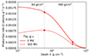 |
Fig. 1. Depth profile of the production rate of 26Al depending on different solar modulation conditions, represented by ϕ. |
The ratio, R, can be a convenient parameter reflecting the heliospheric modulation, ϕ. The relation for 26Al is shown in Fig. 2. It demonstrates that the larger the production rate ratio, R, the greater the heliospheric modulation of GCRs. This simple approach mitigates some imperfections of production models, which can cause systematic over- or underestimations of the absolute production rates.
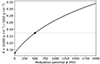 |
Fig. 2. Relation between the ratio, R, of production rates at 400 and 60 g cm−2 and the heliospheric modulation potential, ϕ. The curve is calculated for 26Al produced in the Apollo-15 deep drill core. The circles indicate the scenarios of ϕ = 0 and 500 MV discussed in the text. |
As a next step, we simulated the nuclide content in lunar regolith at depths of 60 and 400 g cm−2. We took into account two main processes: decay and production. We incrementally calculated the nuclide content increase, dN, (in atoms g−1) over the time (age) range of 40 Myr:
 (1)
(1)
where Q is the production rate in atoms g−1 s−1, t and dt are the time and its increment in years (taken as dt = 1 kyr for convenience), and τ is the mean lifetime of the studied cosmogenic nuclide. The boundary condition at an age of 40 Myr (the first data point) is N = 0 atoms g−1, assumed for simplicity, as the time of 40 Myr is sufficient to establish the balance between decay and production for a nuclide with a lifetime of a few million years.
As mentioned above, we assumed that the heliospheric modulation for the period of the interstellar cloud transient is ϕ = 0 MV (no modulation at all), and for the rest of the time it is ϕ = 500 MV. The corresponding time line of the 26Al production rate is shown in Fig. 3, panel (a). There, the Solar System left the cloud 2 Myr ago as estimated by Opher et al. (2024). The transient is assumed to last 1 Myr for the purposes of illustration.
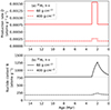 |
Fig. 3. Nuclide 26Al in lunar soil at depths of 60 and 400 g cm−2 over time. Panel (a): Production rate, Q. Panel (b): Nuclide content, N. |
At the current state of old measurements of cosmogenic nuclides in deep drill cores of Apollo missions, we conservatively assess the 95% uncertainty of the estimated ϕ as approximately 10%, that is, σϕ = 50 MV for ϕ = 500 MV. Thus, this provides the least detectable and statistically significant difference in the modulation potential  MV for ϕ of about 500 MV. This estimate allows us to judge whether the estimated observed ϕ from a cosmogenic nuclide of interest (see Fig. 4) indeed remains confidently outside ϕ for the hypothesis of a stable Sun and its heliosphere.
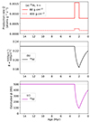 |
Fig. 4. Estimate of the modulation potential as a function of time. Panel (a): Production rate, Q, of 26Al at depths of 60 and 400 g cm−2 over time, the same as in Fig. 3. Panel (b): Ratio of the nuclide content, R, at two depths. Panel (c): Heliospheric modulation potential, ϕ, estimated with R from panel (b) and the curve in Fig. 2, as it would be observed at the given moment of time (age). |
2.2. Modulation potential as a function of modulation boundary
In the standard force-field approach for solving the Parker cosmic ray transport equation (Parker 1965), it is assumed that the effective diffusion coefficient, κ, is a separable function of rigidity, P, and heliocentric radial distance, r, such that κ = k1(P)k2(r), where, for the purposes of this study, it is assumed that k2 = ko(r/ro)γ, with γ being a free parameter, ro a reference distance, usually 1 AU, and ko the value of the effective diffusion coefficient at ro. The modulation potential in the force-field approach can then be written (e.g. Gleeson & Axford 1968; Caballero-Lopez & Moraal 2004; Engelbrecht & Di Felice 2020) as
 (2)
(2)
with Vs being the solar wind speed (assumed here to be constant), and rb the radial distance of the modulation boundary, beyond which no modulation is assumed to occur. A straightforward integration yields
 (3)
(3)
where γ ≠ 1. Taking ϕo to be some average value on the timescale of several lifetimes of 26Al, nominally 500 MV here, a corresponding value of ko as a function of ϕo can be calculated for a modulation boundary, rbo, corresponding to recent heliospheric conditions. This value of ko can then be substituted into Eq. (3) to give a value of the modulation potential, which is a function of the modulation boundary distance, rb, in the past, given by
 (4)
(4)
which implies smaller values for ϕ, and hence less modulation, for values of rb smaller than the present value. We note that the assumption γ = 1 leads to ϕ(rb) = ϕoln[rb/ro]/ln[rbo/ro]. Of course, if rb < Ro, these relations would yield non-physical negative results, so in these cases ϕ is set to zero, corresponding to the no-modulation case. The top panel (a) of Fig. 5 illustrates the modulation potential computed as a function of the modulation boundary radial distance, rb, for different assumptions of the radial dependence of the effective diffusion coefficient, normalised to a value of 500 MV for rbo = 121 AU, the nominal location of the heliopause as detected by the Voyager spacecraft (see, e.g., Richardson et al. 2022, and references therein), which is here assumed to be the current modulation boundary (see, however, Stone et al. 2013; Strauss et al. 2013; Zhang et al. 2015). The choice of γ has a very significant effect when rb > rbo, but less so for the smaller modulation boundaries of interest here.
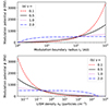 |
Fig. 5. Dependence of the modulation potential on the heliospheric and LISM properties. Panel (a): Modulation potential as a function of modulation boundary, normalised to a nominal value of 500 MV for rbo = 121 AU, for different assumptions of the radial dependence of the effective diffusion coefficient. Panel (b): Modulation potential as a function of interstellar neutral hydrogen density, calculated via Eq. (5), normalised to a nominal value of nH = 0.2 particles cm−3 for present conditions, corresponding to rbo = 121 AU, again for different assumptions as to the radial dependence of the effective diffusion coefficient. See text for details. |
The question now arises as to how to relate rb to the assumed interstellar neutral hydrogen density, nH. This usually requires complex MHD simulations beyond the scope of the present study. However, Müller et al. (2009) provide a relatively simple MHD-motivated estimate for the heliopause boundary based on the simulation results of Müller et al. (2006), so that
 (5)
(5)
where ns = 5 particles cm−3 and Vs = 400 km s−1 denote the solar wind density and speed at ro = 1 AU, respectively (based on a typical value from spacecraft observations, see, e.g., Suess & Tsurutani 2015), nH = ∼0.2 particles cm−3 (Swaczyna et al. 2020; Linsky et al. 2022) denotes the interstellar medium (hydrogen) density, and vism = 26 km s−1 the interstellar medium speed. For the purposes of the present study, ro, HP = 1.52 is chosen to yield a heliopause boundary of 121 AU. Allowing nH to vary makes it possible to express the modulation potential as a function of nH, as is illustrated in the bottom panel (b) of Fig. 5, again shown for various values of γ. Smaller values of nH lead to larger values of rb, hence larger modulation volumes and correspondingly more modulation, the opposite being true for large values of nH. Here, the choice of γ leads to large deviations in ϕ at lower interstellar medium densities, but less so at densities greater than the present-day value of 0.2 particles cm−3, which are of particular interest in this study.
The choice of γ can be made based on radial dependences from the theory for the diffusion coefficient perpendicular to the heliospheric magnetic field (HMF), motivated by the fact that the HMF is azimuthal for most of the heliosphere, so that the radial diffusion of cosmic rays will be predominantly transverse to it (see Engelbrecht et al. 2024). This reasoning should hold over the timescales relevant to this study, as they are too short to expect significant changes in the solar rotation rate (see, e.g., Guinan & Engle 2008), which could in principle make the HMF more radial if the rotation rate were significantly slower than observed currently. For the purposes of the present study, γ = 0.5 is chosen as a preliminary consensus value for the radial dependences of several perpendicular diffusion coefficients derived from various scattering theories that Engelbrecht et al. (2022) present.
This provides the relationship between the heliospheric modulation potential, ϕ, and the density of the LISM, nH, seen in panel (b) of Fig. 5 as the solid black line (γ = 0.5). From there, the minimal density in an interstellar cloud leading to an absence of solar modulation of GCRs at Earth’s orbit, that is, ϕ = 0 MV, is estimated as nH = 2928.5 particles cm−3. This is in line with ∼3000 particles cm−3, the values of Meyer et al. (2006) used by Opher et al. (2024). We notice also the shallow angle of the curve leading to a dramatic decrease in the density, to provide a very minimal modulation: nH = 184.8 particles cm−3 for ϕ = 50 MV. This means that even a large uncertainty in the cloud matter density provides a very small effect on the heliospheric modulation of GCRs, thus providing support for the assumption of ϕ = 0 MV.
3. Results and discussion
Figure 6 illustrates the sensitivity of the method using the long-lived cosmogenic nuclide 26Al in lunar soil for the detection of transient clouds passed by the Solar System within a few million years. The black line in the figure represents the limit of this method for detecting the change in the heliospheric conditions that happened a given time ago and with a given duration. The space above the line indicates that a cloud of the given transient duration and the time to it should be detectable: the average heliospheric modulation, ϕ, should be statistically significantly different from the value corresponding to the Sun in the modern local interstellar environment. Specifically, for this work, it should be lower than 430 MV.
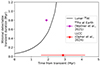 |
Fig. 6. Sensitivity of the method for detecting transient interstellar clouds using 26Al in lunar soil (the black line). We assumed the absence of heliospheric modulation within the cloud, i.e. ϕ = 0 MV, caused by the LISM density, nH = 2.9 ⋅ 103 particles cm−3. The magenta cross indicates the 60Fe enhancement (its peak phase) in sea sediments at the Earth from Wallner et al. (2021) and the red star corresponds to the LLCC estimate from Opher et al. (2024). |
Opher et al. (2024) recently discussed the possible passage of the Solar System through the Local Ribbon of Cold Clouds and specifically considered the LLCC in their work. We also used this cloud as the biggest in the Local Ribbon of Cold Clouds. The velocity of the Solar System relative to the LLCC is estimated by Opher et al. (2024) as 11.4–15.6 km s−1 and the distance to the LLCC is estimated as 22–59 pc. This results in the finding that the Solar System was in this cloud somewhere between 1.6 and 4.2 Myr ago. Unfortunately, the authors do not give an estimate of the duration of such a transient. We used the properties of the LLCC provided by Peek et al. (2011), namely the width of 0.25–0.54 pc conservatively translated by us with the velocities from Opher et al. (2024) to a transient time of 15.6–46.3 kyr. This agrees with the value of about 47 kyr from Müller et al. (2006). Our estimate for the time of the cloud transit (x-axis) and the duration of the transit (y-axis) is plotted in Fig. 6 as a red star.
As one can see, 26Al (lifetime 1.0 Myr) is well-suited for the detection of a transient cloud about 2–4 Myr ago. However, it is still too insensitive to short-duration events (a few tens of thousands of years, in our case) when there is not sufficient time for the increased 26Al production to significantly change the overall content of the nuclide in the regolith in a way that can later be observed. The method based on the lunar nuclide depth profiles does not enable us to directly confirm or reject the passage of the Solar System through a cold, dense, interstellar cloud like the LLCC a few million years ago with a duration of the cloud-crossing event of a few tens of thousands of years. In the current state, the event should last at least a few hundred thousand years to make an observable impact on the current nuclide content. The method’s sensitivity can, however, be greatly improved because it is currently strongly dependent on the uncertainties of measurements of cosmogenic nuclides in the deep drill cores of lunar regolith. These were done in the 1970s to 1980s and modern techniques are likely to reduce them several-fold.
In the next step, we considered the experimental evidence that the Solar system crossed a cold, dense cloud, as proposed by Opher et al. (2024): namely, the discovered peak in the content of 60Fe measured in deep-sea sediments (Wallner et al. 2016, 2021). We estimated the event duration and time of the event from Fig. 1 of Wallner et al. (2021) as roughly 0.8 and 1.9 Myr, respectively. This is a conservative estimate because only the sharp peak at the age of around 2–3 Myr was used. In fact, the 60Fe increase started much earlier (4 Myr ago) and lasted longer (almost 4 Myr) in that record. This data point is also plotted in Fig. 6 as a magenta cross. In this case, the 60Fe event lies well above the sensitivity limits of lunar 26Al and should be clearly seen in the reconstruction of the heliospheric modulation from that nuclide as ϕ = 402 MV. However, this is not the case: reconstructions show a modulation level during the last few lifetimes of 26Al similar to the activity of the Sun during the relatively recent last 11 000 years (e.g. Usoskin et al. 2016; Poluianov et al. 2018; Leya et al. 2021). Using the assumption that the interstellar cloud was much less dense than discussed above, so that it provided only a small reduction in the GCR modulation, statistically indistinguishable from the long-term average ϕ = 500 MV, the required ϕ during the transient should be at least 170 MV, which translates to an LISM density of nH = 7.8 particles cm−3 (rb = 19.4 AU, see Fig. 5 and Eq. (5)). Therefore, it can be concluded that the increase in 60Fe observed in deep-sea sediments cannot serve as evidence of a cold, dense cloud passage, as Opher et al. (2024) propose. The original interpretation by Wallner et al. (2016, 2021) is based on recent nearby supernovae and associated heavy nuclide production with rapid neutron capturing (the so-called r-process), though they also tolerate the hypothesis of the Solar System traversing clouds of 60Fe-enriched dust.
4. Summary
Here, we propose a novel technique whereby the ratios of long-lived cosmogenic nuclide production rates at sufficient depths in lunar regolith cores can be used to ascertain whether periods of anomalously low levels of modulation occurred in the million-year-scale past. Such periods can be the result of the heliosphere having passed through regions of higher density in the interstellar medium, such as molecular clouds, as the Sun orbits the galactic centre. Such clouds have been shown from MHD studies to be able to drastically reduce the size, and hence modulation volume, of the heliosphere, and could thus justifiably lead to an increase in cosmogenic nuclide production. The method proposed here allows for the detection of such events, and, from the inferred modulation potential, can even provide an estimate of the density of the molecular cloud in question, provided some modulation still occurs. There are, however, limitations to the method: uncertainties in the measurements of cosmogenic nuclides made 40 years ago translate into uncertainties in production rates and the modulation potentials inferred from them. Therefore, shorter heliospheric transits of molecular clouds may not be detectable.
This work can be considered as a call for new, high-precision measurements of cosmogenic nuclides, even in old samples from deep drill cores brought to Earth by Apollo missions. This would significantly improve the precision of heliospheric modulation estimates and thus enhance the sensitivity of the method to variations of the heliosphere, thereby potentially leading to new discoveries.
Acknowledgments
N.E.E. would like to thank R.D. Strauss for an insightful discussion on the force field approach. S.P. acknowledges the support from the Research Council of Finland (project GERACLIS, no. 354280) and Horizon-Europe (project SPEARHEAD), he also thanks the North-West University (Potchefstroom, South Africa) for a research visit grant. This work is based on the research supported partly by the National Research Foundation of South Africa (NRF, grant number 137793). Opinions expressed and conclusions arrived at are those of the authors and are not necessarily to be attributed to the NRF.
References
- Agostinelli, S., Allison, J., Amako, K., et al. 2003, Nucl. Instr. Meth. Phys. A, 506, 250 [CrossRef] [Google Scholar]
- Breitschwerdt, D., & de Avillez, M. A. 2006, A&A, 452, L1 [NASA ADS] [CrossRef] [EDP Sciences] [Google Scholar]
- Caballero-Lopez, R. A., & Moraal, H. 2004, J. Geophys. Res.: Space Phys., 109, A01101 [NASA ADS] [Google Scholar]
- Engelbrecht, N. E., & Di Felice, V. 2020, Phys. Rev. D, 102, 103007 [NASA ADS] [CrossRef] [Google Scholar]
- Engelbrecht, N. E., Effenberger, F., Florinski, V., et al. 2022, Space Sci. Rev., 218, 33 [CrossRef] [Google Scholar]
- Engelbrecht, N. E., Herbst, K., Strauss, R. D. T., et al. 2024, ApJ, 964, 89 [NASA ADS] [CrossRef] [Google Scholar]
- Frisch, P. C., & Mueller, H.-R. 2013, Space Sci. Rev., 176, 21 [NASA ADS] [CrossRef] [Google Scholar]
- Frisch, P. C., Redfield, S., & Slavin, J. D. 2011, ARA&A, 49, 237 [CrossRef] [Google Scholar]
- Fuchs, B., Breitschwerdt, D., de Avillez, M. A., Dettbarn, C., & Flynn, C. 2006, MNRAS, 373, 993 [NASA ADS] [CrossRef] [Google Scholar]
- Fuchs, B., Breitschwerdt, D., de Avillez, M. A., & Dettbarn, C. 2009, Space Sci. Rev., 143, 437 [NASA ADS] [CrossRef] [Google Scholar]
- Gleeson, J. J., & Axford, W. I. 1968, Astrophys. J., 154, 1011 [CrossRef] [Google Scholar]
- Guinan, E. F., & Engle, S. G. 2008, Proc. Int. Astron. Union, 4, 395 [CrossRef] [Google Scholar]
- Haud, U. 2010, A&A, 514, A27 [NASA ADS] [CrossRef] [EDP Sciences] [Google Scholar]
- Holzer, T. E. 1989, ARA&A, 27, 199 [NASA ADS] [CrossRef] [Google Scholar]
- Jokipii, J. R., & Kóta, J. 2000, Astrophys. Space Sci., 274, 77 [NASA ADS] [CrossRef] [Google Scholar]
- Jull, A., Cloudt, S., Donahue, D., et al. 1998, Geochim. Cosmochim. Acta, 62, 3025 [NASA ADS] [CrossRef] [Google Scholar]
- Kollár, D., Michel, R., & Masarik, J. 2006, Meteoritics Planet. Sci., 41, 375 [CrossRef] [Google Scholar]
- Kóta, J. 2013, Space Sci. Rev., 176, 391 [CrossRef] [Google Scholar]
- Leya, I., Hirtz, J., & David, J.-C. 2021, ApJ, 910, 136 [NASA ADS] [CrossRef] [Google Scholar]
- Li, Y., Zhang, X., Dong, W., et al. 2017, J. Geophys. Res. Space Phys., 122, 1473 [NASA ADS] [CrossRef] [Google Scholar]
- Linsky, J. L., & Redfield, S. 2023, Front. Astron. Space Sci., 10, 15 [NASA ADS] [CrossRef] [Google Scholar]
- Linsky, J. L., Redfield, S., Ryder, D., & Chasan-Taber, A. 2022, AJ, 164, 106 [NASA ADS] [CrossRef] [Google Scholar]
- McDonald, F. B. 1998, Space Sci. Rev., 83, 33 [NASA ADS] [CrossRef] [Google Scholar]
- Meyer, D. M., Lauroesch, J. T., Heiles, C., Peek, J. E. G., & Engelhorn, K. 2006, ApJ, 650, L67 [NASA ADS] [CrossRef] [Google Scholar]
- Meyer, D. M., Lauroesch, J. T., Peek, J. E. G., & Heiles, C. 2012, ApJ, 752, 119 [NASA ADS] [CrossRef] [Google Scholar]
- Miller, J. A., & Fields, B. D. 2022, ApJ, 934, 32 [NASA ADS] [CrossRef] [Google Scholar]
- Müller, H.-R., Frisch, P. C., Florinski, V., & Zank, G. P. 2006, ApJ, 647, 1491 [CrossRef] [Google Scholar]
- Müller, H. R., Frisch, P. C., Fields, B. D., & Zank, G. P. 2009, Space Sci. Rev., 143, 415 [CrossRef] [Google Scholar]
- Opher, M., Loeb, A., & Peek, J. E. G. 2024, Nat. Astron., 8, 983 [NASA ADS] [CrossRef] [Google Scholar]
- Parker, E. N. 1965, Planet. Space Sci., 13, 9 [Google Scholar]
- Peek, J. E. G., Heiles, C., Peek, K. M. G., Meyer, D. M., & Lauroesch, J. T. 2011, ApJ, 735, 129 [NASA ADS] [CrossRef] [Google Scholar]
- Poluianov, S., Kovaltsov, G. A., & Usoskin, I. G. 2018, Astron. Astrophys., 618, A96 [NASA ADS] [CrossRef] [EDP Sciences] [Google Scholar]
- Potgieter, M. S. 2013, Liv. Rev. Sol. Phys., 10, 3 [Google Scholar]
- Quenby, J. J. 1984, Space Sci. Rev., 37, 201 [CrossRef] [Google Scholar]
- Rancitelli, L. A., Fruchter, J. S., Felix, W. D., Perkins, R. W., & Wogman, N. A. 1975, in Lunar and Planetary Science Conference Proceedings, 6, 1891 [NASA ADS] [Google Scholar]
- Redfield, S., & Linsky, J. L. 2008, ApJ, 673, 283 [Google Scholar]
- Reedy, R. C., & Arnold, J. R. 1972, J. Geophys. Res., 77, 537 [NASA ADS] [CrossRef] [Google Scholar]
- Richardson, J. D., Burlaga, L. F., Elliott, H., et al. 2022, Space Sci. Rev., 218, 35 [NASA ADS] [CrossRef] [Google Scholar]
- Scherer, K., Fichtner, H., Heber, B., Ferreira, S. E. S., & Potgieter, M. S. 2008, Adv. Space Res., 41, 1171 [NASA ADS] [CrossRef] [Google Scholar]
- Schulreich, M. M., Breitschwerdt, D., Feige, J., & Dettbarn, C. 2018, Galaxies, 6, 26 [NASA ADS] [CrossRef] [Google Scholar]
- Slavin, J. D. 2009, Space Sci. Rev., 143, 311 [NASA ADS] [CrossRef] [Google Scholar]
- Snowden, S. L., Heiles, C., Koutroumpa, D., et al. 2015, ApJ, 806, 119 [NASA ADS] [CrossRef] [Google Scholar]
- Stone, E. C., Cummings, A. C., McDonald, F. B., et al. 2013, Science, 341, 150 [NASA ADS] [CrossRef] [Google Scholar]
- Strauss, R. D., Potgieter, M. S., Ferreira, S. E. S., Fichtner, H., & Scherer, K. 2013, ApJ, 765, L18 [NASA ADS] [CrossRef] [Google Scholar]
- Suess, S., & Tsurutani, B. 2015, in Encyclopedia of Atmospheric Sciences, eds. G. R. North, J. Pyle, & F. Zhang, 2nd edn. (Oxford: Academic Press), 189 [CrossRef] [Google Scholar]
- Swaczyna, P., McComas, D. J., Zirnstein, E. J., et al. 2020, ApJ, 903, 48 [NASA ADS] [CrossRef] [Google Scholar]
- Swaczyna, P., Schwadron, N. A., Möbius, E., et al. 2022, ApJ, 937, L32 [NASA ADS] [CrossRef] [Google Scholar]
- Usoskin, I. G., Gallet, Y., Lopes, F., Kovaltsov, G. A., & Hulot, G. 2016, Astr. Astrophys., 587, A150 [NASA ADS] [CrossRef] [EDP Sciences] [Google Scholar]
- Vos, E. E., & Potgieter, M. S. 2015, Astrophys. J., 815, 119 [NASA ADS] [CrossRef] [Google Scholar]
- Wallner, A., Feige, J., Kinoshita, N., et al. 2016, Nature, 532, 69 [NASA ADS] [CrossRef] [Google Scholar]
- Wallner, A., Froehlich, M. B., Hotchkis, M. A. C., et al. 2021, Science, 372, 742 [NASA ADS] [CrossRef] [PubMed] [Google Scholar]
- Wyman, K., & Redfield, S. 2013, ApJ, 773, 96 [NASA ADS] [CrossRef] [Google Scholar]
- Zank, G. P., & Frisch, P. C. 1999, ApJ, 518, 965 [NASA ADS] [CrossRef] [Google Scholar]
- Zhang, M., Luo, X., & Pogorelov, N. 2015, Phys. Plasmas, 22, 091501 [NASA ADS] [CrossRef] [Google Scholar]
All Figures
|
Fig. 1. Depth profile of the production rate of 26Al depending on different solar modulation conditions, represented by ϕ. |
| In the text | |
|
Fig. 2. Relation between the ratio, R, of production rates at 400 and 60 g cm−2 and the heliospheric modulation potential, ϕ. The curve is calculated for 26Al produced in the Apollo-15 deep drill core. The circles indicate the scenarios of ϕ = 0 and 500 MV discussed in the text. |
| In the text | |
|
Fig. 3. Nuclide 26Al in lunar soil at depths of 60 and 400 g cm−2 over time. Panel (a): Production rate, Q. Panel (b): Nuclide content, N. |
| In the text | |
|
Fig. 4. Estimate of the modulation potential as a function of time. Panel (a): Production rate, Q, of 26Al at depths of 60 and 400 g cm−2 over time, the same as in Fig. 3. Panel (b): Ratio of the nuclide content, R, at two depths. Panel (c): Heliospheric modulation potential, ϕ, estimated with R from panel (b) and the curve in Fig. 2, as it would be observed at the given moment of time (age). |
| In the text | |
|
Fig. 5. Dependence of the modulation potential on the heliospheric and LISM properties. Panel (a): Modulation potential as a function of modulation boundary, normalised to a nominal value of 500 MV for rbo = 121 AU, for different assumptions of the radial dependence of the effective diffusion coefficient. Panel (b): Modulation potential as a function of interstellar neutral hydrogen density, calculated via Eq. (5), normalised to a nominal value of nH = 0.2 particles cm−3 for present conditions, corresponding to rbo = 121 AU, again for different assumptions as to the radial dependence of the effective diffusion coefficient. See text for details. |
| In the text | |
|
Fig. 6. Sensitivity of the method for detecting transient interstellar clouds using 26Al in lunar soil (the black line). We assumed the absence of heliospheric modulation within the cloud, i.e. ϕ = 0 MV, caused by the LISM density, nH = 2.9 ⋅ 103 particles cm−3. The magenta cross indicates the 60Fe enhancement (its peak phase) in sea sediments at the Earth from Wallner et al. (2021) and the red star corresponds to the LLCC estimate from Opher et al. (2024). |
| In the text | |
Current usage metrics show cumulative count of Article Views (full-text article views including HTML views, PDF and ePub downloads, according to the available data) and Abstracts Views on Vision4Press platform.
Data correspond to usage on the plateform after 2015. The current usage metrics is available 48-96 hours after online publication and is updated daily on week days.
Initial download of the metrics may take a while.