| Issue |
A&A
Volume 618, October 2018
|
|
|---|---|---|
| Article Number | A179 | |
| Number of page(s) | 32 | |
| Section | Extragalactic astronomy | |
| DOI | https://doi.org/10.1051/0004-6361/201833541 | |
| Published online | 01 November 2018 | |
Extreme quasars at high redshift
1
Instituto de Astrofisíca de Andalucía, IAA-CSIC, Glorieta de la Astronomía s/n, 18008 Granada, Spain
e-mail: This email address is being protected from spambots. You need JavaScript enabled to view it.
2
Istituto Nazionale d’Astrofisica (INAF), Osservatorio Astronomico di Padova, 35122 Padova, Italy
3
CONACYT Research Fellow, Instituto de Astronomía, UNAM, México DF 04510 Mexico
4
Instituto de Astronomía, UNAM, México, DF 04510 Mexico
5
Dipartimento di Fisica & Astronomia “Galileo Galilei”, Università di Padova, Padova, Italy
Received:
31
May
2018
Accepted:
24
July
2018
Abstract
Context. Quasars radiating at extreme Eddington ratios (hereafter xA quasars) are likely a prime mover of galactic evolution and have been hailed as potential distance indicators. Their properties are still scarcely known.
Aims. We aim to test the effectiveness of the selection criteria defined on the “4D Eigenvector 1” (4DE1) for identifying xA sources. We provide a quantitative description of their rest-frame UV spectra (1300–2200 Å) in the redshift range 2 ≲ z ≲ 2.9, with a focus on major emission features.
Methods. Nineteen extreme quasar candidates were identified using 4DE1 selection criteria applied to SDSS spectra: Al IIIλ1860Si IIIλ1892 ≳0.5 and C IIIλ1909/Si IIIλ1892 ≲1. The emission line spectra was studied using multicomponent fits of deep spectroscopic observations (S/N ≳ 40 − 50; spectral resolution ≈250 km s−1) obtained with the OSIRIS at Gran Telescopio Canarias (GTC).
Results. GTC spectra confirm that almost all of these quasars are xA sources with very similar properties. We provide spectrophotometric and line profile measurements for the Si IVλ1397+O IV, C IVλ1549+He IIλ1640, and the 1900 Å blend. This last feature is found to be predominantly composed of Al IIIλ1860, Si IIIλ1892 and Fe III emission features, with weak C IIIλ1909. The spectra can be characterized as very low ionization (ionization parameter, logU ∼ −3), a condition that explains the significant Fe III emission observed in the spectra. xA quasars show extreme properties in terms of C IVλ1549 equivalent width and blueshift amplitudes. C IVλ1549 shows low equivalent width, with a median value of 15 Å (≲30 Å for the most sources), and high or extreme blueshift amplitudes (–5000 ≲ c(1/2) ≲ –1000 km s−1). Weak-lined quasars appear as extreme xA quasars and not as an independent class. The C IVλ1549 high amplitude blueshifts coexists in all cases save one with symmetric and narrower Al IIIλ1860 and Si IIIλ1892 profiles. Estimates of the Eddington ratio using the Al IIIλ1860 FWHM as a virial broadening estimator are consistent with the ones of a previous xA sample.
Conclusions. xA quasars show distinguishing properties that make them easily identifiable in large surveys and potential “standard candles” for cosmological applications. It is now feasible to assemble large samples of xA quasars from the latest data releases of the SDSS. We provide evidence that Al IIIλ1860 could be associated with a low-ionization virialized subsystem, supporting previous suggestions that Al III is a reliable virial broadening estimator.
Key words: quasars: general / quasars: emission lines / quasars: supermassive black holes
© ESO 2018
1. Introduction
Quasars are found over an enormous range of distances (z ∼ 0 − 7.5) in the Universe. For this reason they have occasionally been cited as the ultimate possible standard candles for use in cosmology (see for example the Chapter by in D’Onofrio & Burigana 2009 and the recent reviews by Sulentic et al. 2014b and Czerny et al. 2018). The problem with such a use has been the lack of a clear definition of “quasar” and a contextualization of their diversity. Since 2000 a clearer idea of their nature and diversity has emerged using the 4D Eigenvector 1 (4DE1) formalism. We are now able to identify a main sequence quasar (see (Marziani et al. 2018) for a recent review), and recognize an extreme accretor (xA) quasar population at the end of this sequence (e.g., Marziani & Sulentic 2014; hereafter MS14). This xA population radiating at  ∼1 offer the best opportunity to use quasars for cosmology MS14,(Wang et al. 2014). This paper describes a search for extreme quasars at z ∼ 2.3 built upon an extension of low–redshift 4DE1 studies.
Quasar spectra show diverse properties in measures of line intensity ratios and line profiles. These measures offer multifold diagnostics of emitting region structure and physical conditions (Marziani et al. 2018). Organizing the diversity of quasar properties has been an ongoing effort for many years. Perhaps the first successful attempt was carried out by Boroson & Green (1992). They proposed an Eigenvector 1 scheme based on a principal component analysis of the Palomar-Green quasar sample (see (Gaskell et al. 1999; Sulentic et al. 2000a) for reviews up to the late 1990s). Trends between measures of [O III]λλ4959,5007, optical Fe II emission and full width at half maximum (FWHM) Hβ were found, and appreciation of their importance has grown with time ((Sulentic & Marziani 2015) and references therein). Sulentic et al. (2000b) expanded upon this work and defined a new scheme called 4D Eigenvector 1 (4DE1) with the addition of two new parameters. Principal 4DE1 measures for low-z quasars involve: (1) FWHM of broad line Hβ (excluding any narrow emission component)1; (2) the strength of the optical Fe II blend at 4570 Å normalized by the intensity of Hβ:  = I(Fe II)/I(Hβ); (3) the velocity shift at half maximum (
 ) of the high-ionization line (HIL) C IV
 1549 profile relative to a rest-frame (usually defined by measures of the [O III]λ5007 and or narrow Hβ centroid) and (4) the soft X-ray photon index (Γsoft).
The 4DE1 optical plane (OP), defined by the measures of the FWHM of Hβ and  , shows a reasonably well-defined sequence (a “main sequence” quasar, MS, (Sulentic et al. 2000a; Marziani et al. 2001)). The nomenclature is motivated by an analogy with the role of the stellar main sequence in the H-R diagram which connects observational measures to physical properties (Sulentic et al. 2008). The stellar MS is driven by stellar mass, while the quasar sequence is thought to be driven by Eddington ratio (∝
 , (Marziani et al. 2001, 2003b). Sulentic et al. (2000a) noted a change in all 4DE1 measures near FWHM Hβ = 4000 km s
 in low-z quasar samples (L ≲1047 erg s−1). This change motivated an empirical designation of two quasar populations: Population A with FWHM Hβ ≤ 4000 km s
 ,
,  > 0.5, frequent C IV
 1549 profile blueshifts and sources with a soft X-ray excess, and Population B with FWHM Hβ > 4000 km s
 ,
,  < 0.5, absence of C IV
 1549 blueshift and little or no soft X-ray excess (Bensch et al. 2015). Radio-loud (RL) quasars are strongly concentrated in the Population B domain along with 30% of radio quiet (RQ) sources (e.g.,(Sulentic et al. 2003; Zamfir et al. 2008) and references therein.
Low-ionization emission lines (LILs – Hβ best studied feature) in quasars frequently show asymmetric profiles. The Hβ broad component (HβBC) in Population B sources is usually well described by a double Gaussian profile with one of the components centered on the rest-frame and the second one redshifted by ≈1000–3000 km s (Zamfir et al. 2010), the very broad component (VBC). Population A sources rarely show the redshifted component. High-ionization line (C IV
 1549 best studied prototype) profiles usually show blueward shifts/asymmetries in Population A sources. Pop. B objects also show weak or moderate strength LILs like Fe II and the Ca II IR triplet (Sulentic et al. 2006b; Martínez-Aldama et al. 2015). Usually Population B quasars do not show any strong soft X–ray excess ((Sulentic et al. 2000a; Bensch et al. 2015) and references therein). Largely radio-quiet (RQ) Population A sources usually show symmetric profiles well–modeled with a Lorentz function (Sulentic et al. 2002; Zamfir et al. 2010; Cracco et al. 2016). Population A sources with the narrowest Hβ profiles (< 2000 km s
 ) are often called narrow line Seyfert 1 sources (NLSy1), but in no sense represent a distinct class of quasars (Zamfir et al. 2008; Sulentic et al. 2015).
All of the above description involves quasars with z < 1.0 where moderate to high S/N ground-based spectra exist for significant numbers of sources Hβ (ground based) and C IV 1549 (HST FOS archival data). Within each quasar population systematic trends are revealed in composite spectra of Hβ (Sulentic et al. 2002; Zamfir et al. 2010) and C IV (Bachev et al. 2004). Sulentic et al. (2002) defined Pop. A subclasses A1, A2, A3 and A4 in order of increasing intervals of 0.5
 have been defined. Extreme Population A sources in bins A3 and A4 (xA) involve quasars with very strong
  ≳ 1.0. This criterion is applicable only to sources at low redshift. This study involves searching for higher redshift analogs of such extreme quasars. At high redshift (z > 2) the spectral range used to define sources in the 4DE1 (FWHM Hβ,
  ) context are lost unless NIR spectra are available for Hβ (Marziani et al. 2009). Many C IV spectra in the intermediate and high-z range are available in the SDSS and BOSS archives although low S/N often precludes detailed analysis.
The 4DE1 provides a consistent picture of quasar observational properties in low-z samples: beginning with the low- and broad FWHM Hβ, involving high black hole mass “disk-dominated” quasars. As we move along the sequence we encounter sources whose spectra show narrower LIL profiles, lower ionization spectra, and blueshifted C IV
 1549 profiles providing evidence of strong HIL emitting outflows: “wind-dominated” quasars (Richards et al. 2011). Eddington ratio (convolved with the effects of orientation) appears to be the physical parameter driving systematic changes of observational properties along the quasar MS (Sulentic et al. 2000a; Marziani et al. 2001; Boroson 2002). The main sequence observational trends can be interpreted as driven by small
  , higher
  (young? high accretors) toward the high
  end of the sequence. The xA sources cluster around
  ≈ 12. This would imply that the low-z xA sources are the “youngest” (less massive than Pop. B) quasar population radiating at the highest Eddington ratios (Fraix-Burnet et al. 2017).
There is a growing consensus that sources at the high  end of the MS are accreting at the highest rates, and are expected to be close to the radiative limit per unit black hole mass (Sun & Shen 2015; Du et al. 2016a,b; Sniegowska et al. 2018). If this is the case, xA quasars acquire a special meaning. While Population A HILs are dominated by blue shifted emission associated with outflows, the presence of almost symmetric and unshifted LILs (Balmer lines, but also Paschen lines, La Franca et al. 2014) indicate the coexistence of a LIL emitting region that is virialized. Since
  tends toward a constant limiting value (Mineshige et al. 2000), xA quasars can be considered as “Eddington standard candles.” If so that, if
  can be retrieved under the virial assumption, an estimate of the luminosity becomes possible since
  ∝L/
∝L/ (Wang et al. 2013; La Franca et al. 2014),MS14. This approach is conceptually analogous to the use of the link between the velocity dispersion in virialized systems (i.e., the rotational velocity of HI disks in spiral galaxies Tully & Fisher 1977). Initial computations for samples of 100–200 low-z quasars (≲1) confirm the conceptual validity of the “virial luminosity” estimates (Negrete et al. 2017, 2018), although scatter in the distance modulus is still too large to draw meaningful inferences for cosmology.
4DE1 trends can also be helpful for interpreting high-L and high-z quasars, although there are two caveats. At high redshift, z ∼ 2, the majority of sources show large FWHM due to a bias in luminosity (Sulentic et al. 2014a, 2017): quasars with luminosities comparable to the low-z low-L sources are still too faint to be efficiently discovered. More fundamentally, there is a minimum possible FWHM Hβ at fixed luminosity, if the line emitting region is virialized and its size follows a scaling law with luminosity. In practice this means that at logL ≳ 47, all lines have to be broader than FWHM 2000 km s . By the same token the FWHM limit for Population A becomes luminosity dependent. The limit established at 4000 km s
 is valid only for low-z, relatively low-L quasars. Sources with larger FWHM and emission line properties similar to the ones of the low-z xA quasars have been found at high-z and high-L ((Negrete et al. 2012),MS14). Another important issue at high-L concerns the HIL blueshifts. While at low-L large blueshifts (vr ≲ −1000 km s
 ) are confined to Pop. A (Sulentic et al. 2007; Richards et al. 2011), at high-L they are ubiquitous (Coatman et al. 2016; Bischetti et al. 2017; Bisogni et al. 2017), even if Pop. A sources still show the largest blueshift amplitudes among all quasars (Sulentic et al. 2017; hereafter S17). At any rate, several recent studies confirm that Hβ, observed in NIR spectra in quasars at z ≳ 1 shows fairly symmetric and unshifted profiles suggesting that the broadening is mainly due to virial motions of the line emitting gas (Marziani et al. 2009; Bisogni et al. 2017; Shen et al. 2016; Vietri et al. 2018),S17. We will show in this paper that this is probably true also for high-L xA sources.
Goals of this paper include testing the effectiveness of 4DE1 selection criteria for identifying high  xA sources at z ∼ 2.4. This will enable us to analyze spectral properties of the identified xA quasars in the rest-frame UV region. A sample of candidate xA sources (hereafter GTC-xA) was observed with the Gran Telescopio de Canarias (GTC) using the OSIRIS spectrograph. We apply the 4DE1 selection criterion defined by MS14 using UV diagnostic ratios: Al IIIλ1860/Si III
 1892 ≳ 0.5 and C III
 1909/Si III
 1892 ≲ 1.0. The selected sources are intended to represent an xA population for which
  is expected to be larger than 1, with no limitation on line FWHM. The sample selection is described in Sect. 2. The observations and the data reduction are presented in Sect. 3. We perform a multicomponent fitting and build Monte Carlo (MC) simulations to estimate measurement uncertainties (Sect. 4 and Appendix B). Spectra and line measures are presented for the 1900 Å blend, the blend C IV
 1549 + He II
 1640, and the Si IV
 1397 region in Sect. 5. A comparison with control samples at low-z and or L is described in the Sect. 6.1. A composite spectrum for the GTC-xA sample (Sect. 5.1) allows us to carry out a comparison with low-z and low-L samples (Sect. 6.2). We discuss the low-ionization spectra and identify Fe III and Fe II features that are prominent in our spectra (Sects. 6.3 and 6.4). After estimating the main accretion parameters (Sect. 6.5), we briefly analyze the relation of xA sources to Weak Line Quasars (WLQs) – a related class of quasars with extreme properties (Sect. 6.6).
xA sources are especially important because they are the quasars radiating at the highest luminosity per unit mass. The extreme radiative properties of xAs make them prime candidates for maximum feedback effects on host galaxies. We briefly analyze the possibility of significant feedback effects in Sect. 6.7. We conclude the paper with some consideration on the possible cosmological exploitation of xA quasars at high-z (Sect. 7).
2. Sample description
2.1. GTC-xA sample
MS14 extracted 3000 quasar spectra from the SDSS DR6 archive which provided coverage of the 1900 Å blend for sources in the redshift range 2.0 < z < 2.9, with g < 19.5. Intensity measures of Al IIIλ1860, Si III 1892 and C III
 1909 were carried out with an automatic SPLOT procedure within the IRAF reduction package. The majority of SDSS spectra are quite noisy making them suitable for identifying samples of candidate sources, but not providing accurate spectroscopic measures (Sulentic & Marziani 2015). A preliminary selection of extreme Eddington candidates was made and sources were then vetted according to the xA selection criteria (Al IIIλ1860/Si III
 1892 ≳ 0.5 and C III
 1909/Si III
 1892 ≲ 1.0). MS14 considered the brightest candidates with moderate S/N (≥15) spectra, leaving 58 candidate xA quasars whose relative Al IIIλ1860, Si III
 1892 and C III
 1909 intensities satisfied the selection criteria, but whose S/N was too poor to make an accurate measurement of individual lines in the 1900 Å blend. Hence the need for new GTC spectroscopic observations. This paper present an analysis of 19 of the sources that constitute our GTC-xA sample.
Table 1 gives source identifications and basic properties including: redshift and uncertainty (Cols. 2 and 3), emission line used for the redshift estimate (Col. 4), apparent V magnitude and absolute B magnitude MB (Cols. 5 and 6) as given in Véron-Cetty & Véron (2010), and (g − r) color index from the SDSS photometry (Col. 7). Column 8 identifies other observed features like its classification as BAL (Broad Absorption Line) or mini-BAL quasar, and the radio properties, if they are detected. Low-z studies (Zamfir et al. 2008) define a radio-loud (RL) quasar with a radio/optical flux ratio log  ≳ 1.8 (Kellermann et al. 1989), or better a radio power measure logPν > 31.6 [erg s−1 Hz1], independent of uncertainties in optical flux measures.
  was obtained normalizing the k−corrected radio flux at 1.4 GHz by the k−corrected B magnitude. Two radio-detected sources exceed the
  limit with the third one close to the limit. Only for SDSSJ233132.83+010620.9 was possible to estimate the radio spectral index from one observation at 8.4 GHz (Cegłowski et al. 2015): αr ≈ 0.44, that places it in the compact steep-spectrum radio domain. SDSSJ234657.25+145736.0 has only a low-resolution NRAO VLA Sky Survey (NVSS) map available. In this case, Pν and
  have been computed assuming αr = 0. All of them exceed the log Pν limit, then we could have three RL quasars in GTC-xA sample. Since low-z RL are almost never found in the xA domain in 4DE1, it is possible either that the three radio detected sources are not xA extreme accretors or that high-z Pop. A quasars are more frequently RL. At this point the three RL sources in the sample must be treated with caution.
Source identification and basic properties of the GTC-xA quasars.
2.2. The FOS-A, S14-A, and FOS-xA “control” samples
The quasars in the GTC-xA sample are thought to be highly accreting, with an average bolometric luminosity of logL∼ 47 [erg s ]. Absolute magnitude MB ≈ −26, before extinction correction, corresponds to a comoving space density of ∼10−6 mag−1 Mpc−3 just beyond the turnover at the high luminosity end of the 2dF luminosity function (Boyle et al. 2000).
In order to compare the behavior of the GTC-xA sample, we consider the FOS sample from Sulentic et al. (2007) as a control sample at low-L and low-z. For the sake of the present paper, we restrict the control FOS sample to 28 Pop. A RQ sources covering the C IV and 1900 Å blend spectral range and with previous measures for the Hβ profile and  (Marziani et al. 2003a). 23 objects are classified as Pop. A1–A2 sources (henceforth FOS-A sample) and five as xA sources (hereafter FOS-xA sample) including I Zw 1. The FOS sample has a typical bolometric luminosity logL ∼ 45.2 [erg s−1] and a redshift z≲ 0.5.
The sample presented in Sulentic et al. (2014a, hereafter S14 covers a similar range in redshift (z ∼ 2.3, corresponding to a lookback time of ≈10 Gyr), and are in turn a factor approximately ten less luminous (logL ∼ 46) than the GTC-xA sample. S14 is representative of a general population of faint, moderately accreting quasars that are also found at intermediate redshift (Fraix-Burnet et al. 2017). S14 includes both Pop. A and B sources, but no xA sources. Restriction to the eleven Pop. A quasars (hereafter S14-A) offers a high-z counterpart to the FOS-A sample, and therefore suitable for a comparison between xAs and a sample of Pop. A quasars of moderate L at z ∼ 2 − 2.5, that represents a population expected to be relatively common (Φ ∼ 10−6 mag−1 Mpc−3).
3. Observations, data reduction and extinction estimation
3.1. Observations and data reduction
Long slit observations were carried out in service mode using the OSIRIS spectrograph at the 10.4 m GTC telescope of the Roque de los Muchachos Observatory. Grisms R1000B and R1000R with 2 × 2 CCD binning were used for the observations, depending on the redshift of the source. The majority of the observations employed R1000B that covered the wavelength range from 3650–7400 Å with a reciprocal dispersion of 2.1 Å per pixel (R ≈ 1000). In our highest z sources, SDSS J105806.16+600826.9, SDSS J125659.79-033813.8, and SDSS J233132.83+010620.9 with z ≈ 2.94, 2.98 and 2.63, respectively, we used the R1000R grism with reciprocal dispersion of 2.6 Å pixel−1 and spectral coverage 5100–10 000 Å. These two spectral ranges correspond the rest-frame region covering the UV spectral features of interest such as the Si IV 1397, C IV
 1549 and the 1900 Å blend. The spectra were obtained with an 0.6 arcsec slit width oriented at the parallactic angle in order to minimize atmospheric differential refraction. Table 2 contains a summary of the observations including: SDSS identification, observation date, grism employed, total exposure time for the three individual exposures on each source, seeing estimated from the FWHM of field stars in the acquisition image, and the estimated S/N in the 1450 Å continuum region on the blue side of C IV
 1549.
1549.
Log of observations.
Data reduction was carried out in a standard way using the IRAF package. Bias subtraction and flat-fielding correction were performed nightly. Wavelength calibration was obtained using Hg+Ar and Ne lamps observed with the same configuration and slit width used for source observations. Wavelength calibration rms was less than 0.1 Å. We checked the wavelength calibration for individual exposures with sky lines before source extraction, background substraction, and final combination. Scatter of the sky line wavelength peaks was ≲20 km s . This value provides a realistic estimate of the wavelength scale uncertainty including zero point error. Spectral resolution estimated from FWHM of the skylines is ∼230 km s
 and 250 km s
 for grisms R1000B and R1000R, respectively.
Instrumental response and flux calibration were obtained nightly with observations of the spectrophotometric standard stars Ross 640, GD24-9, Feige 110, Hiltner 600, and G158-100. In order to improve flux calibration, we also included two additional flux standard stars, LDS749B and HZ21, as target objects. They were observed with both grisms and two slits: 0.6 arcsec b (as used for quasar observations) and 5 arcsec. A comparison between the different slits gives a change in the absolute flux calibration ∼10%. Spectra were corrected for light losses due to the narrow slit width employed and also to differential light loss as a function of wavelength. Taking into account the ratio between the slit width and the seeing during an observation allowed correction for the scale factor and for the wavelength dependence of the seeing following the method described by Bellazzini (2007). Telluric absorptions, that affect our spectra mainly beyond 7600 Å, were also corrected using the standard stars to obtain a normalized template of the absorption features. The template was shifted if needed, and scaled for each individual source in an iterative and interactive procedure, until the residuals in the telluric correction were negligible. Spectra were finally deredshifted as explained in Sect. 4.1.
3.2. Extinction estimation
It is visually apparent from examining our spectra that some of them (e.g., SDSSJ021606.41+011509.5, Fig. A.3) show a flatter continuum than cannot be modeled with a single power-law over the observed spectral range. This effect, as well as the presence of BALs, has been interpreted in the literature as indicating the presence of dust or internal reddening. In order to assess the importance of internal reddening on the observed fluxes and derived magnitudes in our xA sample, we have estimated the reddening in each source by fitting its UV continuum with quasar templates excluding spectral regions with broad emission lines (e.g., Lyα, Si IV 1397, C IV
 1549 and the 1900 Å blend). We used four QSO templates: (1) a median composite spectrum representative of the xA quasar population and built with extreme accretor sources identified in the SDSS DataBase by MS14 excluding BALs; (2) a template involving the composite FIRST Bright Quasar Survey spectrum (FBQS; Brotherton et al. 2001; 3) the composite spectrum provided by Harris et al. (2016) with BOSS spectra of quasars in the redshift range 2.1 < z < 3.5, and (4) the SDSS composite quasar spectra (Vanden Berk et al. 2001). We reddened the templates using an SMC extinction law (Gordon & Clayton 1998) which appears to be the most appropriate reddening law for modeling quasar spectra (York et al. 2006); galleranietal10. We assumed a RV coefficient of 3.07 for the extinction law.
In general, best fits were obtained with the xA composite although there were no appreciable differences and all the fittings yielded similar results. For the majority of sources (twelve) no additional extinction was needed and the continuum was well represented by the templates. In six cases the reddening has a significant effect on the spectrum, amounting to AV = 0.1 to AV = 0.32. Table 3 reports reddening estimates parametrized by the AV value. In the case of SDSSJ220119.62-083911.6, classified as BAL, the spectrum shows a broad and deep absorption in the blue wings of C IV 1549, Si IV
 1397 and Ly
 with an evident flattening of the continuum at wavelengths shorter than 1600 Å. However, from 1700 Å the spectrum shows a similar slope to the templates and does not show evidence for reddening. Hence no internal reddening was applied to this source and the continuum at 1350 Å needed for estimation of the luminosity was obtained by extrapolating the power law of the fit applied to the red spectral region.
Extinction measures for the xA sources.
4. Data analysis
4.1. Redshift determination
Accurate redshift estimates are very important because redshift defines the quasar rest-frame from which emission line shifts can be measured. Shifts are particularly important for HILs like C IV 1549 (e.g.,(Gaskell 1982; Espey et al. 1989; Carswell et al. 1991; Marziani et al. 1996)). Redshift estimates are chiefly obtained from narrow emission lines (or the narrow core of Hβ) for low-z sources (e.g.,(Eracleous & Halpern 2003; Hu et al. 2008)). In the UV region covered by our spectra of z ≈ 2.3, narrow LILs are not present. We must resort to broad LILs and estimate the redshifts using three features: Al IIIλ1860, C II
 1335 and O I
 1304+Si II
 1306. The strongest and hence most often detected LIL involves Al IIIλ1860, which emerged in lower z studies as a kind of UV surrogate Hβ (Bachev et al. 2004). While often detected, it is always part of the 1900 Å blend albeit on the blue end of it. Although Al IIIλ1860 and Si III
 1892 are blended lines, they are stronger than C II
 1335 and O I
 1304+Si II
 1306 and in many of the spectra their peaks are clearly seen. We performed a multicomponent fit for each source, considering all the lines in the region of the 1900 Å blend (see Sect. 4.2). The peaks of Al IIIλ1860 and Si III
 1892 were unconstrained in intensity in the fitting and the adopted model of the blend was the one with minimum χ2. C II
 1335 is the only isolated LIL in the observed UV range and is detected in only five sources (e.g., SDSSJ021606.41+011509.5, see Fig. A.3). The O I
 1304+Si II
 1306 blend is also well seen in a few sources where C II
 1335 is detected. In the rest of the sample these lines are too weak to be useful and are often affected by absorption features.
We constructed synthetic Gaussian profiles for C II 1335 and O I
 1304+Si II
 1306 lines using the IRAF task MK1DSPEC assuming FWHM ∼ 4000 km s
 . We computed a redshift from the peak of the synthetic features. When the Al IIIλ1860 redshift was compared with the one of C II
 1335 and O I
 1304+Si II
 1306, we find three cases where the difference is less than 100 km s
 . In these cases, we kept the redshift value determined by the C II
 1335 and O I
 1304+Si II
 1306 (label I and II in Table 1). In the cases where the difference is larger than 100 km s
 , we considered the redshift given by Al IIIλ1860 and Si III
 1892 (label III in Table 1), since the peak of these lines is clearly observed. The uncertainty reported in Col. 4 of Table 1 has been computed from the redshift difference between C II
 1335, O I
 1304+Si II
 1306, and Al IIIλ1860+Si III
 1892.
1892.
4.2. Multicomponent fitting
Emission lines can be distinguished by their ionization potential (IP). The UV range covered in our spectra is populated by intermediate (IP ∼ 20–40 eV) and high ionization lines (IP > 40 eV). They offer an opportunity to characterize the behavior of different ionic species at the same time. In order to analyze the emission lines in our spectra, we carried out multicomponent fits using the SPECFIT routine from IRAF (Kriss 1994). This routine simultaneously fits the continuum, and emission/absorption line components. The best model is indicated by the minimum χ2 over a spectral range where all components are included.
The main continuum source in the UV region is thought to arise from the accretion disk (Malkan & Sargent 1982). In the absence of extinction the continuum can be modeled by a single power-law over the full observed spectral range. However, due to the presence of absorptions (BAL sources) or dust extinction the continuum is flattened out in several sources (Sect. 3.2). Whenever possible, we fit the entire spectra range with a single power-law or a linear continuum. Otherwise we estimate locally the continuum. We divide the observed spectral range in three parts, which are centered on the most important emission lines relevant to our work.
R EGION 1: 1700–2200 Å. This range is dominated by the 1900 Å blend which includes Al IIIλ1860, Si III 1892, C
 1909 and Fe III lines (see Sect. 5.6 and Appendix B for Fe III line identification). On the blue side of the blend Si II
 1816 and N III
 1750 are also detected. Al, Si and C are intermediate–ionization lines (IIL) and according to Negrete et al. (2012; hereafter N12) can be well-modeled with Lorentzian profiles. The strengths of the three lines are allowed to vary freely in our SPECFIT model. FWHM Al and Si were assumed equal, while FWHM C was unconstrained. Si
 1816 and N III]
 1750 were also modeled with Lorentzian profiles with flux and FWHM allowed to vary freely. All Lorentzian profile peaks were fixed at rest-frame. Fe II makes an important contribution in the range 1715–1785 Å. We tried to use templates available in the literature (Brühweiler & Verner 2008; Mejía-Restrepo et al. 2016), but we could not reproduce the observed contribution. If that template is scaled to reproduce these features, the Fe II emission around the Mg II
 2800 line would be overestimated by a large factor. On the converse if the template is normalized to Fe II in the proximity of Mg II
 2800, the Fe II emission in the spectral region 1700–2200 Å is negligible. We therefore decided to fit isolated Gaussian profiles for Fe II at 1715 and 1785 Å. Their flux and FWHM vary freely. Fe III emission makes a larger contribution than Fe II and appears especially strong on the red side of the 1900 Å blend. We modeled the emission of this ion with the Vestergaard & Wilkes (2001) template and included an extra component at 1914 Å following N12 (the motivation for this choice is discussed in Sect. 6.3). Around 2020–2080 Å we were forced to include extra Gaussians in order to obtain a good fit (we found excess emission with respect to the Fe III template). The flux and FWHM of the features at 2020–2080 Å were allowed also to vary freely.
R EGION 2: 1450–1700 Å. The C IV 1549 emission line dominates this region and is accompanied by He II
 1640, O III
 1663 and Al II
 1670. The broad component (BC) of C IV is modeled by a Lorentzian profile fixed at the rest-frame. The flux of the CBC is free and FWHM is assumed to be the same as Al IIIλ1860 and Si III]
 1892. All the C IV profiles in our sample show a blueshift and or blueward asymmetry. In order to model it with SPECFIT, we used one or two blueshifted skewed Gaussian profiles. The flux, FWHM, asymmetry and shift were unconstrained. He II
 1640 was modeled assuming components similar to those of C IV
 1549: Lorentzian and skewed Gaussian profiles for the BC and blueshifted components, respectively. The FWHM, shift and asymmetry were assumed equal to those of C IV
 1549, but the flux varies freely. O III
 1663 and Al II
 1670 were also modeled with unshifted Lorentzian profiles with their fluxed and FWHM varying freely.
R EGION 3: 1300–1450 Å. The dominant emission in this region involves Si IV 1397+O IV (the 1400 Å blend), and is accompanied by weaker Si II
 1306, O I
 1304 and C II
 1335 lines. The underlying assumption of the blend modeling is that the BC emission is dominated by Si IV
 1397 due to collisional deexcitation of the inter combination O IV multiplet (Wills & Netzer 1979), while the blue shifted component is due to an inextricable contribution of both O IV+Si IV
 1397. The Si IV
 1397+O IV feature is a high-ionization blend, and shows a blueshifted, asymmetric profile not unlike C IV
 1549. The broad component was modeled with the same emission components of C IV, whenever possible (in several cases the blue side of the Si IV
 1397+O IV blend was strongly contaminated by absorption features making a good fit impossible), with only the flux varying freely. In the case of strong absorption the blueshifted emission was modeled independently from the one of C IV.
For lines that are composed of more than one component (C IV 1549, He II
 1640 and Si IV
 1397+O IV) the total profile parameters were also computed: FWHM, centroid at half maximum (
 ), and asymmetry index (AI) defined by Zamfir et al. (2010). Unlike the SPECFIT components, these parameters provide a description of the profile that is not dependent on the model decomposition of the profile.
Figure 1 shows the multicomponent fitting made to the composite spectrum obtained by combining the normalized spectra of the GTC-xA sample (see Sect. 5.1 for a complete description). The bottom panels of the figure present the fits performed on the Si IV 1397, C IV
 1549 and Al IIIλ1860 spectral regions of the continuum subtracted spectrum. Residuals of the fits are shown in the lower part of the bottom panels. Spectra and multicomponent fits for the individual 19 quasars analyzed in this paper are shown in Figs. A.1–A.19. Error estimations of blended emission lines were evaluated by building Monte-Carlo (MC) simulations as explained in Appendix B.
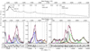 |
Fig. 1. Top panel: rest-frame composite spectrum (see Sect. 5.1). Abscissa corresponds to vacuum rest-frame wavelength in Å, while ordinate is in arbitrary intensity. Dot-dashed vertical lines identify the position at rest-frame of the strongest emission lines. Bottom panels: multicomponent fits after continuum subtraction for the 1400 Å blend, C IV |


5. Results
5.1. Composite spectrum
We constructed a median composite spectrum from the individual observations in order to emphasize the main emission features (composites efficiently remove narrow absorption lines) and carry out a comparison with other samples (see Sect. 6.2). The composite GTC-xA spectrum corresponds to the median of all the normalized individual spectra including BALs. This simple approach produced a spectrum that reflects the behavior of the xA objects (see Fig. 1).
In xA sources, the 1900 Å blend of the composite spectrum shows a high contribution of Al IIIλ1860 and Si III] 1892 compared to C III]
 1909. Most of the emission on the red side of Si III]
 1892 can be attributed to Fe III excess in addition to the template, which is required to minimize the fit χ2. A fit with C III]
 1909 only (with no Fe IIIλ1914) would leave a large residual at 1915–1920 Å. Strong Fe III emission is confirmed also by the prominent bump at 2080 Å predominantly ascribed to the Fe III multiplet #48.
On the blue side of C IV 1549, a smooth and shallow through is due to the combined effect of broad absorption lines that are frequent shortwards of C IV
 1549. The emission profile of C IV
 1549 is in any case almost fully blueshifted, as observed in the majority of sources. Also the Si IV
 1397 median profile shows a blueshift asymmetry even if it is affected by the heavy absorptions frequently observed on the blue side of this line. The net effect is that Si IV
 1397 +O IV appear more symmetric because their blue wings are truncated by narrow and broad absorptions. The composite also clearly shows the prominent low-ionization features associated with C II
 1335, and O I
 1304 blended with Si II
 1306. C IV
 1549 +He II
 1640 shows low equivalent width, close to the boundary of WLQs (see Sect. 6.6). The composite spectrum is especially helpful for the increase in S/N that allows us to trace the broad and faint He II
 1640 profile, which shows a flat topped appearance. It is interpreted in the multicomponent fits as due to a strong blueshifted component, blended with a faint BC and with O III
 1663 and Al IIλ1670.
5.2. Consistency of selection criteria for xA sources
Using lines in the 1900 Å blend, MS14 proposed that xA sources with  > 1 show flux ratios Al IIIλ1860/Si III
 1892 ≳ 0.5 and C III
 1909/Si III
 1892 ≲ 1. Our sample was selected considering these criteria applied to SDSS noisy spectra previously excluded by MS14. The high S/N spectra of the GTC sample presented in this work confirm the defining criteria for the identification of the highly accreting sources in the UV range. Figure 2 shows the location of the 19 sources of our sample in the plane defined by C III
 1909/Si III
 1892 vs. Al IIIλ1860/Si III
 1892. In order to compared the behavior of the xA with the rest of the Pop. A, in Fig. 2 are also represented control samples (FOS-xA, FOS-A and S14-A) described in Sect. 2.2.
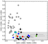 |
Fig. 2. Relation between intensity ratios Al IIIλ1860/Si III |


Comparing the flux ratios shown by the low and high-z Pop. A and xA samples, like MS14 have done, we observe a clear difference between the two kind of populations. The FOS-xA and GTC-xA samples show flux ratios different to the ones of FOS-A and S14-A samples. The GTC-xA sources occupy a very well defined region in the bottom right side of the panel, while the Pop. A sample occupy the left top space. Two of the objects (SDSSJ222753.07-092951.7 and SDSSJ125659.79-033813.8, ∼10% of our sample) do not rigorously satisfy the selection criteria, although they present similar spectral properties to ones observed in the rest of the sample. The measured line ratios are actually borderline: the Al IIIλ1860/Si III 1892 ratio of the BAL SDSSJ125659.79-033813.8 is ≈0.40 ± 0.10, the C III]
 1909/Si III]
 1892 ratio of SDSSJ222753.07-092951.7 is ≈1.36 ± 0.23. Therefore the two quasars will be considered along with all other GTC-xA sources.
5.3. 1900 Å blend
Table 4 reports emission lines measurements corresponding to the 1900 Å blend region: Al IIIλ1860, Si III] 1892, C III]
 1909, N III]
 1750 and Si II
 1816. The first column lists the SDSS name. The equivalent width (W), flux (F) and FWHM of Al IIIλ1860 are reported in Cols. 2, 3, and 4, respectively. Equivalent width and flux are reported for Si III]
 1892 in Cols. 5 and 6, since its FWHM is assumed equal to the one of Al IIIλ1860. W, F and FWHM of C III]
 1909 are reported in Cols. 7, 8 and 9, respectively. They are followed by the flux of the two faint features outside of the blend: N III]
 1750 and Si II
 1816 (Cols. 10 and 11). All the parameters have uncertainties at 1σ confidence level, which were obtained from the MC simulations. The MC method followed to estimate the uncertainties is explained in Appendix B.
Measurements in the 1900 Å blend region.
In several instances the Al IIIλ1860 doublet is partly resolved and is assumed to be at the rest-frame along with Si III] 1892. In general, the Al IIIλ1860 flux, FWHM and W can be estimated with good accuracy as the doublet can be efficiently deblended save for the cases that the lines are very broad (FWHM ≳ 6000 km s
 ). Al IIIλ1860 is well fit with a symmetric and unshifted Lorentzian. Typical uncertainties in FWHM are ≲10%. Only in one case (SDSSJ084036.16+235524.7) there is evidence for a blue asymmetry in the 1900 Å blend although the Al IIIλ1860 BC can be isolated with good accuracy. The fraction of the blueshifted to the total Al emission would of ≈0.25, small compared to a median value of ≈0.46 for C IV. The presence of a blue shifted component in Al IIIλ1860 is a rare occurrence. Only in one source of the S17 sample shows evidence of a blueward Al IIIλ1860 excess (HE0359-3959,(Martínez-Aldama et al. 2017)).
The peak of the 1900 Å blend is often not in correspondence of the C III] 1909 wavelength. If the blend of Si III], C III] and Fe III is peaked, the peak is preferentially redshifted beyond 1909 Å. The 1900 Å blend profile may show excess emission on its red side (see e.g., SDSSJ021606.41+011509.5, Fig. A.3). In these cases, we suggest that the main contribution is coming from the Fe IIIλ1914 line, modeled with a Lorentzian in excess to the Fe III template (Sects. 5.6 and 6.4), or by unresolved Fe III emission.
The weaker lines N III] 1750 and Si II
 1816 are detected in about two thirds of the sample, for example they are both prominent in the case of the quasar SDSSJ021606.41+011509.5. The N III]
 1750 line shows a wide range in W. It is not detected in four sources but the detections show W in the range 0.5–5 Å.
5.4. Cλ1549 and He λ1640
Measurements associated with the emission lines of the C IV] 1549 spectral region are reported in Table 5. The first column lists the SDSS name. Column 2 reports the rest-frame specific continuum flux (fλ) at 1350 Å. No error estimate is provided; the inter calibration with different standard star spectra suggests an uncertainty around 10%, which should include all main source of errors in the absolute flux scale. Columns 3–7 tabulate W, flux, FWHM, centroid at half intensity (
 ) and asymmetry index (A.I.) of the C IV
 1549 total profile (broad plus blueshifted components). Columns 8 and 9 list the equivalent width and F of the broad component of C IV. Its FWHM is not reported, because it is assumed to be the same as FWHM Al IIIλ1860, due to the BC have to be emitted by the same zone. The equivalent width, F, FWHM and
  of the blueshifted component of C IV are given in Cols. 10–13, respectively.
Measurements on C IVλ1549 region.
Table 6 reports the measurements associated with He II 1640 and contaminant lines. Columns 2–7 list the W and flux of He II
 1640 total profile, He II
 1640 BC and He II
 1640 blue shifted component respectively. Column 8 lists the O III
 1663 + Al II
 1670 flux. The last column reports the N IV
 1486 flux. The N IV
 1486 flux is highly uncertain due to absorption lines and to the blending with the blue wing of C IV, then in many of the cases only upper limits are reported.
Measurements on He IIλ1640 region.
On average, the He II 1640 total flux is ∼20% that of C IV
 1549. Since the typical W C IV
 1549 ≈ 10 − 15 Å, the typical W He II
 1640 is around ≈3 Å distributed over a broad profile with 4000 ≲ FWHM ≲ 11 000 km s
 . The weakness of the He II
 1640 emission with respect to C IV
 1549, with C IV
 1549/He II
 1640 ≈5 − 6 ≳ 3 is out of the question. It is important however to stress that our approach tends to maximize the contribution of the CBC to the total C IV
 1549 emission. This may lead to an overestimation of the C IV
 1549/He II
 1640 BC ratio. Nevertheless, in several cases (e.g., SDSS J214009.1–064403.9) we observed a significant C IV
 1549 emission at rest-frame, implying that the C IV
 1549/He II
 1640 estimate ≈5 − 6 is a safe one. We mention the C IV
 1549/He II
 1640 ratio because its value is rather high for the low ionization parameter expected in the emitting regions, if metallicity is solar or slightly supersolar (Sect. 6.3, N12).
An important feature in our spectra involves the strong blueshifts and asymmetries associated with the HILs. In ∼50% of our sample, the C IV blueshifted component contributes ∼50% of the total profile. He II 1640 also shows a highly blueshifted component, contributing ∼60% of the total flux. The A.I. values also support the presence of outflows: the blueshifted component pumped by radiative forces is more prominent than the virial component located at rest-frame. This is a major difference between high-ionization lines (e.g., C IV
 1549) on the one side, and low and intermediate–ionization lines on the other (e.g., Al IIIλ1860). The last one are basically symmetric and show no evidence of large shifts with respect to the rest-frame.
An indication of the strength of the outflow is provided by the shift amplitude of the blue shifted component or by the shift amplitude of the total C IV profile measured by the centroid at half intensity,  . The most negative values indicate stronger blueshifts suggesting stronger outflows. BAL quasars tend to show smaller values of
  (closer to 0) in the C IV profile, due to the presence of the absorption features in the blue side of the profile. The non-BAL quasars show values 1000 ≲ ∣
  ∣ ≲ 5000 km s
 . He II
 1640 shows even stronger asymmetries than C IV
 1549, although they could be related to the faintness of He II
 1640 and the deblending uncertain of broad and blue components. The strong outflows could be important for feedback effects on the host galaxy (Sect. 6.7).
5.5. Siλ1397+Oλ1402
Table 7 reports the values of the emission lines in the Si IV 1397+O IV spectral region (1400 Å blend). The blue side of the 1400 Å spectral region is seriously affected by absorption lines. The Si IV
 1397+O IV blend is formed by high-ionization lines. A blueshift asymmetry is expected in the profile, but in ∼40% of the sample the blueshifted component can not be detected due to strong absorption lines. In the rest of the sample, the measurements of the
  and FWHM are also affected to the ever-present absorptions. C II
 1335 and O I+S IIλ1304 are also affected by the absorption. In the majority of the sample, they cannot be detected or their flux uncertainty is large.
Measurements on 1400 Å blend region.
5.6. The Fe and Fe emission
Fe II emission is usually not very strong in the range 1700–2100 Å, even in the case of the strongest optical Fe II emitters. Only a few features are detected at ∼1715 Å, 1785 Å and 2020 Å. We modeled these individual features with single Gaussians, without using a model template emission. On the other hand, the Fe III emission has a most important role in xA sources. It was modeled using the scaled and broadened template of Vestergaard & Wilkes (2001) based on I Zw 1. However, it is not enough to reproduce the observed Fe III emission. We added two extra emission component at 1914 and 2080 Å (modeled by two Gaussians), to account for the line of Fe III UV #34 line that may be enhanced by Ly fluorescence, and for the broad hump at 2080 Å, mainly ascribed to the blended features of Fe III UV #48. Most relevant Fe II and Fe III features between 1700 and 2100 Å are individually discussed Appendix C.1.
Table 8 reports the equivalent widths and the fluxes of the most important UV Fe II multiplet #191 (Fe II 1785 Å) and the ones of the total Fe II emission, that is the sum of the Fe II features described above: at 1715, 1785 and 2020 Å. Table 9 reports equivalent widths and fluxes of the most important individual features ascribed to Fe III (1914 and 2080 Å) and the total Fe III emission: the sum of the individual features and the template contribution in the full range. It is interesting to note that Fe III emission is almost always stronger than Fe II, by a factor of ∼2–3. The strong Fe III emission will be discussed in Sect. 6.4 and Appendix C.2.
Flux and equivalent width of Fe II contribution.
Flux and equivalent width of Fe III contribution.
5.7. The origin of the C 1549 line broadening
The GTC-xA sample shows a very tight correlation between FWHM and  of the total C IV
 1549 profile (Fig. 3). The best fitting to our new sample is
  ≈(−0.613 ± 0.081)⋅FWHM + (1893 ± 545) km s
 . This relation is consistent within uncertainties with the one found by S17 involving Pop. A sources. The range of blueshifts is from ≈ –1000 to –5000 km s
 in both cases; however, the distribution of the GTC-xA is weighted in favor of larger shifts and broader FWHM with respect to the one of S17. As noted by S17, the correlation of Fig. 3 justify the decomposition of C IV
 1549 profile into the BC and a blueshifted excess, which becomes the dominant source of broadening in the case of the largest FWHM.
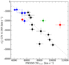 |
Fig. 3. Relation between the |


5.8. Alλ1860 as a high redshift virial estimator
Identification of a UV virial estimator for high redshift quasars (z≳ 2) has been an important quest for several years (e.g., review by (Marziani et al. 2017b)). Once Hβ is lost to ground based spectroscopy, Mg II 2800 can be exploited up to z ∼ 2.0 (Trakhtenbrot & Netzer 2012); shenliu12; marzianietal13. C IV
 1549 is the obvious candidate for quasars beyond z ∼ 2.0, but the C IV line profiles often show large blue shifts and or asymmetries whose amplitude is a function of source location along the 4DE1 sequence and also of luminosity S17. This implies that
  estimation using FWHM C IV can be uncertain by a large factor (Sulentic et al. 2007; Netzer et al. 2007; Mejía-Restrepo et al. 2018). There have been several recent attempts to account for the bias associated with the non-virial broadening of C IV
 1549 (Park et al. 2013; Matsuoka et al. 2013; Brotherton et al. 2015; Denney et al. 2016; Coatman et al. 2017), however no correction yields safe
  estimates especially if Population A and B sources are not considered separately. We focus here on extreme Pop. A (xA) sources and attempt to use Al IIIλ1860 as an Hβ virial surrogate. The first composites of low-z FOS sources suggested that Al IIIλ1860 becomes more prominent at the extreme Pop. A end of the 4DE1 sequence (Bachev et al. 2004). The Al IIIλ1860 line shows a FWHM similar to the one of Hβ, which suggests that both lines are emitted in similar dynamical condition (Negrete et al. 2013). Analysis of VLT ISAAC + FORS spectra of high-z Pop. A sources (Marziani et al. 2017b) show also that FWHM Al IIIλ1860 agrees well with FWHM Hβ. Previously, the emission lines associated with the 1900 Å blend such as Al IIIλ1860 or C III]
 1909 were avoided due to severe blending (Shen & Liu 2012), and the 1900 Å blend remains poorly studied to date. Our earlier work motivated us to identify xA source candidates and to obtain high S/N spectra of C IV
 1549 and the 1900 Å blend. In the majority of the xA candidates observed so far the Al IIIλ1860 profile is well defined and is not strongly affected by absorption features (see Sect. 5.3).
The left panel of Fig. 4 shows a comparison between FWHM C IV 1549 and FWHM Al IIIλ1860 for the xA sample. The ratio between both FWHMs as a function of the FWHM Al IIIλ1860 is shown in the bottom part of the panel. Coatman et al. (2017) proposed an empirical correction to the C IV profile to obtain the contribution associated with the virial component. Its factor is based on a measure of the C IV blueshift analog of the
  we measure. We then applied a correction to the FWHM C IV
 1549 proportional to
  C IV
C IV 1549 to correct for the excess broadening due to the blueshifted component. The result is shown in the right panel of Fig. 4. All C IV
 1549 measurements have FWHM larger than FWHM Al IIIλ1860 before correction. Sources with FWHM Al IIIλ1860 ≈3000 km s
 show a bias factor of ≈2.5–3 in C IV FWHM, implying almost an order-of-magnitude excess in
  estimates. After correction, even if the bias is almost zeroed, we find no significant improvement over the uncorrected panel. This is especially true when we examine the spectra of the 4-6 sources with largest differences with FWHM Al IIIλ1860. C IV, in most of them, is affected by absorptions. Most of the highest confidence measures involve the cluster of sources in the lower left corner of the figure, which can be argued to be the highest confidence xA sources. However the sample is too small to allow us to go further. In a forthcoming paper comparing FWHM Hβ and FWHM Al IIIλ1860 measures for our low and higher z samples (Marziani et al., in prep.), we find a clear correlation for Pop. A sources. FWHM Al IIIλ1860 provides the safest equivalent of FWHM Hβ for virial estimation in Pop. A sources.
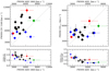 |
Fig. 4. Relation between the FWHM Alλ1860 and FWHM C |


5.9. Prevalence and properties of absorbed systems
The C IV 1549 emission line profile of our GTC-xA sources frequently shows absorptions: only in 9 cases the profile is not contaminated by deep broad absorptions and in only 5 cases the profile is not affected by any narrow or broad absorption. In order to ascertain whether our sample suffers from unusually strong line absorption compared to a general quasar population at 2.0 ≲ z ≲ 2.9, we considered estimates of the absorption index (AI) and Balnicity index (BI) as defined in Scaringi et al. (2009). The AI (Hall et al. 2002) includes semibroad absorptions continuously detected over a range of at least 1000 km s
 , from 0 to –29 000 km s
 ; the BI (Weymann et al. 1991) measures contiguous absorption features over 2000 km s
 in the range of –25 000 to –3000 km s
 , and is intended to identify quasars with broad through features almost certainly not associated with external absorbers. Table 10 reports the AI and BI measures for our sample. Large C IV
 1549 BI absolute values (≲−1000 km s
 ) are associated with Pop. A and with “strong” BALs with large equivalent widths and high up to terminal velocity, while mini-BALs are also found at low-z among Pop. B and RL objects (Sulentic et al. 2006a). Trump et al. (2006) provide both AI and BI measurements obtained from a SDSS DR3 catalog containing 5719 quasars in redshift range z ∼ 2 − 2.6 (Schneider et al. 2005). There are 542 sources with C IV
 1549 BI < 0 suggesting ≈ 9.5% for “strong” BAL sources, consistent with conventionally quoted prevalence values for BAL QSOs. In the GTC-xA sample, 5 over 19 sources show C IV
 1549 BI < , 0. If we also include one source with C IV BI = 0 (SDSSJ144412.37+582636.9), but with strong absorption in the blue side of Si IV
 1397+O IV blend at 1400 Å and BI ≪ 0 (see Fig. A.13), we obtain a prevalence of BAL QSOs around 25–30%. AI is less than 0 in 10 out of 19 sources of the GTC-xA sample; about 30% of Trump et al. (2006) satisfy the same condition. If one considers that about 1/2 of SDSS quasars are Pop. A quasars (Zamfir et al. 2010), the prevalence of strong BAL sources should be doubled to ∼20%. We can therefore conclude that the GTC-xA sample does not show an unusually large fraction of intrinsically absorbed systems, possibly at a prevalence somewhat higher than the general quasar population.
Balnicity and Absorption indices.
6. Discussion
6.1. Equivalent width distributions
Figure 5 shows a comparison between the equivalent width distributions of Al IIIλ1860, Si III] 1892, C IV
 1909 and C
 1549 for the GTC-xA sources and the three control samples: the low-z (FOS-A and FOS-xA) and the high-z (S14-A) samples. The Al IIIλ1860 line of the GTC-xA shows an enhancement relative to the other samples (upper left panel). The Al III values distribution for the GTC-xA sources is significantly different more than 6σ respect to the ones observed in FOS-A and S14-A, according to a T-test (6.7σ and 6.1σ, respectively). In fact, a Kolmogorov-Smirnov (KS) test gives a very low probability of being equal population between GTC-xA, and FOS-A and S14-A (8 × 10⁻⁶ and 5 × 10⁻⁶, respectively). Meanwhile, there is no statistically significant difference between the two Pop. A samples (FOS-A and S14-A) or the two Pop. xA (GTC-xA and FOS-xA) samples.
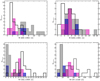 |
Fig. 5. Rest-frame equivalent width distributions of the Al IIIλ1860, Si III |


The Si III] 1892 equivalent width (upper right panel) covers a wide range of values with no statistical significant difference between the samples. Only at a level of 2σ, the GTC-xA shows slightly higher values of W Si III]
 1892 than FOS-A sample. But neither the T-test nor the KS test yield a significant probability of being different populations.
Instead, in the GTC-xA sample the W C distribution (bottom left panel) appears to be markedly weaker than a Pop. A. Both T-test and KS-test give significant differences at 6.5σ and 5.2σ level for the GTC-xA sample to be a different population respect to FOS-A and S14-A respectively. The probability according to the KS test is very low (3.2 × 10⁻⁶ and 1 × 10⁻⁴, respectively). In xA sources C III] 1909 is weak and blended with the Fe III contribution, to the point of not being clearly detectable in several cases. On the other hand, in the Pop. A samples (FOS-A and S14-A) this ion is perfectly appreciable by naked eye and specially prominent in Pop. B sources (e.g., (Bachev et al. 2004; Kuraszkiewicz et al. 2004))
Bottom right panel of Fig. 5 shows a comparison between the equivalent width distributions of C IV 1549 for xA and Pop. A sources. xA values are the ones with the lowest W C IV
 1549 among Pop. A sources, with a wide majority of sources distributed below ∼40 Å. On the converse, the FOS-A and S14-A samples show a much broader distribution, with no evidence of a systematic difference between them, within the limitations of the relatively small sample sizes. The statistical tests gives a significant difference between GTC-xA and FOS-A and S14-A at 5σ and 7σ, and a KS-test a low probability (∼10−5) to be the same population.
These histograms give a first hint to the fact that xA quasars show a different spectroscopic behavior compared with the one shown by samples of the full Population A. Due to there are not any significant differences in the equivalent width distributions of two xA samples (GTC-xA and FOS-xA) and neither between the two Pop. A samples (FOS-A and S14-A), we can consider a sample with 24 xA sources (19+5) and 34 Pop. A sources (23+11). A comparison of the Al IIIλ1860 equivalent width of the 24 xA respect to 34 Pop. A sources shows a significant difference between them at a level of 7.8σ with a low probability to be the same distribution (7 × 10⁻⁸). There is also a statistically significant difference in the distributions of C III] and C IV 1549, but in the opposite direction: values of the xA sources are significantly lower than Pop. A (6.6σ and 5σ level respectively with probabilities lower than 2 × 10⁻⁷).
6.2. Composite spectra at low and high-z
With the objective of highlight main features observed in the xA spectrum and make a comparison with control samples, we built a composite spectrum using the full GTC-xA sample. Multicomponent fits and its analysis are shown in Sect. 5.1. At the top level of Fig. 6 is represented the composite GTC-xA spectrum. It clearly shows an enhancement of Al III and Si III], in contrast with the weakness of C III], which has mean W C III] ∼ 4 Å. Also, Fe III becomes the largest contribution in the red side of the 1900 Å blend, which is also prominent in the Fe III feature detected at ∼2080 Å. Another noticeable feature is the almost fully blueshifted C IV 1549 profile, which shows a low equivalent width. A blueshift is also observed in Si IV
 1397+ OIV
 1402, although in this case the profile is more symmetric due to the presence of strong absorptions in its blue side. As we point out in Sect. 5.4, He II
 1640 is very weak with a flat topped appearance profile. Low-ionization features, C II
 1335 and O I
 1304+Si II
 1306, are also clearly appreciated.
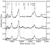 |
Fig. 6. From top to bottom, rest-frame composite spectra of the GTC-xA, FOS-xA, and S14-A. Intensity units are arbitrary flux. The GTC-xA and FOS-xA have been displaced by a constant value for clarity. |
In order to compare the general behavior of xA sources, we also built composite spectra for two comparison samples: FOS-xA and S14-A samples, middle and bottom level of Fig. 6, respectively. A multicomponent analysis was also applied to composite control samples. The width line of Al IIIλ1860 in FOS-xA (∼2740 km s ) is narrower than GTC-xA (∼4500 km s
 ). The average bolometric luminosity of the FOS-xA sample is ∼2.4 × 1045 erg s−1 and ∼1047 erg s
 for the GTC-xA, therefore a FWHM change can be associated with the higher luminosity in the GTC-xA sample.
The S14-A composite spectrum shows a comparable luminosity (logL ≈ 46) than the FOS-xA, and a similar redshift that GTC-xA sample. S14-A shows a strong and symmetric C IV 1549 profile with a median equivalent width of 47 Å, more than two times large than the median values obtained in xA samples: 14 and 23 Å for GTC-xA and FOS-xA, respectively. Conversely, the 1900 Å blend of S14-A composite spectrum is dominated by C III] and Si III] profiles. The xA samples show a weaker C III], with median values of equivalent width 2.6 Å for GTC-xA, 1.8 Å for FOS-xA and 11 Å for S14-A. Also they shows a stronger Al IIIλ1860 that Pop. A samples, with the next median values: 7 Å for the GTC-xA, 6 Å for FOS-xA and 2 Å for S14-A. Other notable features of xA sources include a smaller He II
 1640, as well as a higher ( OIV
 1402+ Si IV
 1397)/C IV
 1549BC ratio. Features like O I
 1304+Si II
 1306 and C II
 1335 are also clearly observed, supporting the inference of a low-ionization degree for xA objects (see Sect. 6.3). There is a fundamental caveat between GTC-xA and S14-A samples: among the faint sources of S14-A there is no xA sources. A systematic difference in
  of ≈2 can be accounted, if the Eddington ratio of GTC-xA sources is
  ≈1 and if the S14-A are instead radiating at
  ≈0.3 (Sulentic et al. 2014a), without invoking any effect of luminosity.
6.3. A low–ionization spectrum with prominent Fe
The UV spectral range provides several diagnostic ratios that can constrain physical parameters. For instance the C III] 1909/Si III]
 1892 and Al IIIλ1860 Si III
 1892 ratios are sensitive to hydrogen density, C IV
 1549/Al IIIλ1860 and C IV
 1549/Si III]
 1892 to ionization, and He II
 1640/C IV
 1549 and ( OIV
 1402+Si IV
 1397)/C
 1549 to metallicity (N12(Negrete et al. 2013, 2014)),. The diagram of Fig. 7 has been computed from an array of CLOUDY 13.05 (Ferland et al. 2013) simulations covering the range in ionization parameter −4.5 ≤ logU ≤ 0 and density 7 ≤ nH ≤ 14 cm
 , with steps of 0.25 dex. A total of 551 simulations were carried out assuming a standard AGN continuum appropriate for Pop. A, a column density Nc = 1023 cm−2 and a metallicity of 100 Z⊙. The median flux ratios given by Al IIIλ1860/Si III]
 1892, C IV
 1549/Al IIIλ1860, and C IV
 1549/Si III]
 1892 converge toward logU ≈ −3 and log
  ≈13 [cm−3]. The suggestion of low-ionization and high density is in agreement with the previous study of two xA sources by N12. Consistently with the inference of high density, C
 1909 is usually weak although not entirely negligible with a log C
 1909/Si
 1892 ≈ − 0.42. Due to the critical electronic density of the C III]
 1909 is nH = 1010 cm
 , this line is expected to be collisionally suppressed with respect to Al IIIλ1860 and Si III]
 1892, as it is shown by the GTC-xA composite spectrum. The strong Fe III contribution observed in the GCT-xA sources also supports the existence of a very low–ionization spectrum, logU ≤ −2. A more detailed analysis of Fe III emission is presented in Appendix C.
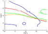 |
Fig. 7. Isocontours in the plane log of ionization parameter (U) versus log of hydrogen density ( |


The intensity ratios considered above are not strongly sensitive to metallicity except for the He II 1640/C IV
 1549 and the (O IVλ1402+Si IV
 1397)/C IV
 1549 ratios. According to CLOUDY simulations, at solar metallicity we expect C IV
 1549/He II
 1640 ≈1 for the low-U and high density solution, which is very far from the value that we derive for the xA sample (∼0.19). A possible solution is offered by a large increase in metallicity above solar values. The He II
 1640/C IV
 1549 is the ratio between a recombination and a collisionally excited line: at high-Z, the metals absorb a larger fraction of the ionizing flux, and the He recombination line become weaker. This effect leads to a decrease of the He II
 1640/C IV
 1549 over the value expected at solar Z (Hamann & Ferland 1993, 1999). In this case, the Z-sensitive He II
 1640/C IV
 1549 would be small (∼0.2) even at low-ionization. An increment in the metallicity to Z ≈ 100 Z⊙ gives such low He II
 1640/C IV
 1549 ratios (Fig. 7). The value Z ≈ 100 Z⊙ may appear unrealistically high. However, N12 found evidence of high-Z, as well as of possible abundance anomalies. It appears reasonable to assume very high values of Z for xA sources: Pop. A sources at low-z and high-z have N V
 1240/C IV
 1549 and (O IVλ1402+Si IV
 1397)/C IV
 1549 implying Z ≳ 10 Z⊙(Shin et al. 2013), S14. The median ratio Si IV
 1397/C IV
 1549 ∼ 1 may suggest a metallicity significantly higher than 10 times solar for the GTC-xA sample. The high Si IV
 1397+O IVλ1402/C IV
 1549 ratio also supports this suggestion. In agreement with the interpretation of Hamann & Ferland (1999), the equivalent width of He II
 1640 is extremely low, making the line almost undetectable above noise.
We should also consider that our approach may overestimate the C IVBC intensity, as it attempts to maximize its contribution attempting to account for the red side of the profile, even when the profile if almost fully blue shifted. There is the possibility that the C IVBC is significantly weaker. A slightly lower value of Z = 50 Z⊙ is again in agreement with the observations assuming an overestimation of the C IVBC intensity by factor of two. Therefore, a Z value of several tens Z⊙ might be considered as a lower limit if we consider a systematic overestimation of the C IVBC. It is unlikely that the overestimate might be much larger than a factor of two, as the C IVBC is clearly detectable while He II 1640 equivalent width is extremely low. More precise inferences require dedicated photoionization computations beyond the scope of this paper.
6.4. Evidence of 2080 Å enhancement
Several sources show a significant excess with respect to the template at around ∼2080 Å, indicating that UV #48 is selectively enhanced with respect to the “normal” emission in xA sources as represented by Vestergaard & Wilkes (2001) template. In eight sources the equivalent width of the feature in excess respect to the template is W(2080) ≳5 Å. This excess is evident from the spectra, and is even more outstanding because the HILs in the adjacent spectral regions are of low equivalent width. A mock profile built from the transition of multiplet Fe III UV # 48 between the terms a5S − z5Po, assuming relative intensity for optically thin transitions (Kovačević et al. 2010) accounts for the 2080 Å feature: the mock profile resulting from the lines broadened to 4000 km s is a feature at ≈2073 Å with total FWHM ≈ 5000 Å, consistent with the observations.
Figure 8 shows the equivalent width of the Fe IIIλ1914 and of the Fe II UV #191 multiplet versus the equivalent width of the 2080 Å feature. Only ten sources satisfy the detection limit we imposed at W ≈ 1Å. Strong Fe IIIλ2080 is usually associated with strong Fe IIIλ1914. According to an orthogonal fit taking into account errors in both axis, these two emission lines follow the relation Fe III1914 = (0.46 ± 0.14) ⋅ Fe III2080+(1.29 ± 0.55), which verified the null hypothesis of a slope different from 0 at 3.3σ significant level. There is a clear relation, although the errors associated with Fe IIIλ1914 are high because of the blend with C III] 1909 and the contribution of the Fe III template. On the another hand, the Fe IIUV #191 is generally rather weak, but the five cases with a clear detection (W≳ 2 Å) are associated with strong 2080 Å features. An orthogonal fit gives a relation Fe IIUV = (0.27 ± 0.06) ⋅ Fe IIIλ2080 + (0.57 ± 0.30) with a slope different from 0 at a 4σ significance level. This relation considers measurements with W> 1.0 Å of both Fe II UV #191 and Fe IIIλ1914 (Fig. 8). A fluorescence mechanism (described in Appendix C.2) may account for the selective enhancement of the 2080 Å feature.
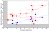 |
Fig. 8. Relation between intensity of the Fe III feature at 2080 Å with Fe UV 1785 Å (blue) and Fe IIIλ1914 (red). Squares, up and down triangles, and circles mark the normal, BAL, mini–BAL and RL quasars, respectively. The gray shaded area indicates an approximate detection limit. Blue and red lines mark the orthogonal fit for each case. |
6.5. Estimates of the accretion parameters
6.5.1. Bolometric correction
There has been no accurate determination of the bolometric correction (hereafter B.C.) specific to xA sources. An attempt has been made to compute the bolometric correction from the model SEDs of MS14. MS14 suggested that the difference in the optical, UV, X range between a typical NLSy1 and an extreme NLSy1 is about 10% (see their Sect. 6.1.2.3). It is unlikely that the uncertainty in the B.C. is much larger than ≈20% (at 1σ confidence level). SDSS quasars have with B.C.1350 = 3.5 and a scatter ∼20% (Richards et al. 2006). SDSS quasars are however an heterogenous sample composed by quasar of different spectral types. On the contrary, the GTC-xA sample is composed by similar sources. If we consider 27 spectra of sample 3 of MS14, that is at redshift in the range 2.0–2.6, the rms averaged between ≈1100 and 2900 Å is ≈10%.
Considering that the bulk of the ionizing energy is coming from the big blue bump in correspondence of the Lyman limit, the SED is not significantly different from the one of Mathews & Ferland (1987). The MS14 SED differs from the reference Mathews & Ferland (1987) SED only for the slope in the X-ray domain, and yields a B.C.1350 ≈ 5.4. The B.C. value is consistent with the one of Elvis et al. (1994). The value of Elvis et al. (1994) may perhaps provide a more appropriate comparison, as the sources in that paper implied a detection from the IPC instrument on board the Einstein observatory (Giacconi et al. 1979), that is in the soft X-ray domain. Bolometric luminosities LBol of the GTC-xA sources are presented in Table 11. They have been computed through the monochromatic luminosities at 1350 Å (λLλ(1350 Å)) and a B.C. = 5.4 ± 0.6. A more careful estimate would require a detailed analysis of the mid- and far-IR domain, where part of the accretion luminosity is reradiated, and is deferred to an eventual work.
Accretion parameters.
6.5.2. Black hole mass
We estimate black hole mass ( ) using the UV C IV scaling relation of Vestergaard & Peterson (2006), Eq. (7)) applied to FWHM(Al III)3. The Al III profile is usually not affected by the strong outflows often observed in the C IV
 1549 profile, thus providing a good approximation to the virial motion of the BLR (e.g.,(Marziani et al. 2017b) see also Sect. 5.8). We adopt
  ,AlIII as the virial mass estimator. Second column of Table 11 shows the
  estimations. Typical formal uncertainties in the estimation of the masses, through error propagation, are about 25% taking into account an uncertainty of 10% in the flux at 1350 Å, and including the estimated errors for the FWHM Al IIIλ1860.
The GTC-xA sample covers a black hole mass range of 8.8 ≤  ≤ 9.8
≤ 9.8  , with a median value of ⟨
 ⟩ ∼ 9.2
  . The GTC-xA sample is covering the high-
 counterparts of the FOS-xA sample. Also these values confirm the well–know tendency of larger black hole mass (∼109
 ) at high redshift (z ≈ 2; Shemmer et al. 2004; Netzer et al. 2007; Trakhtenbrot & Netzer 2012), a redshift-dependent selection effect common to all flux-limited samples (Sulentic et al. 2014a).
6.5.3. Eddington ratio
Eddington ratios ( ) have been calculated based on masses obtained from the FWHM Al III, explained in previous section and following the relation:
  ≈ 1.5 × 1038 ⋅ (
 /
/ ) [erg s
 ], as recommended by Netzer & Marziani (2010).
  values for our sample are reported in Table 11. Applying the usual method of propagation of errors and using previous formulae, the typical mean uncertainty in the Eddington ratio is about 30–35% (only in one case the estimated error is larger than the 50%, in SDSSJ233132.83+010620.9
  ≈ 0.5 ± 0.3).
The average  value for the GTC-xA sample is ⟨
 ⟩ ≈ 0.66, comparable to the one obtained for I Zw 1, a prototype highly accreting quasar at low-z. An appropriate sample for a comparison is also the sample #3 of MS14 that involves xA quasars in the redshift range 2 ≤ z ≤ 2.6 with the Al IIIλ1860 used as a virial broadening estimator. The obtained average
  of the GTC-xA sample is consistent with the value obtained for sample #3 of MS14 (
 ≈ 0.7), once the estimates are computed with the same bolometric correction (5.4 in this work versus 6.3 in MS14), and the same
  constant (MS14 used 1.3 × 1038 erg s−1). A Welch-test on the average
  confirms that two averages are not significantly different, and therefore the xA nature of the sources in the present sample.
The scatter in  in the GTC-xA sample after extinction correction is σL/LEdd∼ 0.47 which is somewhat above the one of sample-#3 of MS14 (σL/LEdd ≈ 0.16), although this may be in part due to the small size of the GTC-xA, with only 19 objects. Also the larger scatter in FWHM may contribute to the
  scatter: average FWHM Al III ∼4220 ± 900 km s
 for MS14 versus an average FWHM Al III ∼4720 ± 1600 km s
 for the GTC-xA sample. As an example, SDSSJ144412.37+582636.9 has a FWHM Al III ∼8080 km s
 which yields the minimum
  value (0.1) in the sample. Additionally this source is a mini-BAL with clear absorptions in its spectrum (see Fig. A.13) introducing additional uncertainties in the extinction correction. In the absence of an orientation correction, a large scatter in the observed FWHM translates into a large scatter in
  .
.
A correlation between the  shift and
  (Sulentic et al. 2017) implies that highest
  values are associated with the highest
  . Figure 9 shows the plane
  vs.
vs.  , where GTC-xA sources occupy a fairly extreme position, where also I Zw 1 is located. Two third of the 11 sample (unabsorbed sources) have
  ≲ − 2000 km s
 , and the blueshifts distribution is more skewed toward high
  values than in the sample of S17. Comparing with the HE sample (Sulentic et al. 2017) and FOS-xA and FOS-A sample (Sulentic et al. 2007), we observe that FOS-xA sources (the pale blue squares around
  ∼1) also cover a similar domain of blueshift amplitudes, while Pop. A sources show lower amplitude shifts, −900 km s
 on average. This diagram provides further support to the idea that the Eddington ratio is the physical driver of the outflows, and that xA sources are associated with high Eddington ratio values.
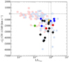 |
Fig. 9. Behavior of the centroid at 1/2 of total C |


6.6. Weak-lined and xA quasars
The Weak-Line Quasars (WLQs) show very low equivalent width in the C IV 1549 and other UV emission lines (Diamond-Stanic et al. 2009; Wu et al. 2012; Shemmer et al. 2010). A standard definition of WLQ involves sources with W(C IV) ≤ 10 Å. WLQs also show strong Fe II emission and C IV blueshift. Luo et al. (2015) provides one of the largest samples of WLQ candidates, with detailed measures on shifts and W of C IV for 21 of them. It is an almost exclusively RQ sample as are 4DE1 Population A, and especially xA quasars. Most WLQ candidates are high-z making estimates of source rest-frame uncertain in many cases. When Hβ measures are available (Plotkin et al. 2015; Sulentic et al. 2007, 2017), we confirm that WLQs belong to the Population A domain of 4DE1 with
  ≳ 1.0, independently of z and L (Fig. 9 of (Marziani et al. 2016)). At least 80% of WLQs are xA sources and, if doubtful cases (e.g., affected by absorptions, so most likely not real WLQs) are excluded all WLQs might belong to the xA population. The majority of WLQ show FWHM Hβ ≳ 2000 km s
 . WLQ are simply Pop. A sources with strong
  , high amplitude C IV blueshift and the lowest values for W C IV.
According to the standard WLQ definition our GTC-xA sample includes three WLQs, excluding BALs. If we consider the prevalence of WLQs among xAs in different samples, we found: four out of 42 in MS14; one out of three (S17); 3 out of 13 in the present sample (excluding BAL and mini-BAL QSOs), and two out of ten (sulenticetal07), for a total fWLQ = nWLQ/nxA = 10/68 ≈ 15%.
As we see in Sect. 6.1, the peak of the GTC-xA W C IV 1549 distribution is slightly above 10 Å (see also bottom right panel of Fig. 5). There is no solution of continuity at W C IV
 1549 ≈ 10 Å. WLQs are located at the low end of the W C IV
 1549 distribution of the GTC-xA sources and there is no suggestion that they constitute a special class. Moreover, as in the case xA sources, WLQs are characterized by extreme outflow velocities. Figure 10 shows the W C IV
 1549 vs. C IV
 1549 shift domain for the 19 GTC-xA sources of our sample and several WLQs, Pop. xA and Pop. A samples: 19 WLQs from Luo et al. (2015), six WLQs from Plotkin et al. (2015), four WLQ from Wu et al. (2012) which includes PHL 1811 from Wu et al. 2011, three Pop. xA and eleven Pop. A from Sulentic et al. (2017), and five xA and 23 Pop. A from S07. The measurements in our samples are the centroid at half maximum, while Luo et al. (2015) consider interactive measurement, presumably of the peak shift. In the context of the present analysis, we expect that the effect may not be relevant because, in the case of the largest blueshift, the total profile is shifted so that peak and centroid at half maximum yield consistent values.
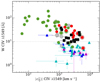 |
Fig. 10. Relation between rest-frame equivalent width of C IV |


The distributions of xA and WLQ blueshifts are largely overlapping, with an excess of WLQs showing blueshifts in the range 5000–10 000 km s . A trend between W C IV
 1549 and C IV
 1549 shift amplitude is suggested, in the sense that the blueshift amplitude appears to increase among weaker C IV
 1549 emitters. It is important to consider that this is part of a general trend among quasars, with a much higher statistical significance if Pop. A and B at high luminosity are included (Marziani et al. 2016).
Restricting attention to xA and WLQs means to consider only the extreme end of the equivalent width-shift distribution. Both xAs and WLQs show a coupling between physical and dynamical conditions of the outflowing gas which seems a well-defined, common phenomenon affecting outflow-dominated sources S17. WLQs can therefore interpreted as extreme xA sources in the context of 4DE1. The previous discussion also validates the assumption that at least the wide majority (if not all) of RQ WLQs are xA quasars. In addition, it suggests that WLQs are an ill-defined class, and that their observational properties should be analyzed within the context of the wider class of xA sources.
At the present time we suggest that observational biases may be playing a serious role. If one considers the data for the most extreme WLQs, extremely low W and extremely high C IV blueshifts, we find that some of the lowest W values in Fig. 10 involve sources with C IV absorptions, that reduce W C IV, and UV redshift uncertainties, that affect estimates of C IV shifts (Luo et al. 2015). Only a few WLQ candidates have data available for the Hβ region (Plotkin et al. 2015). Two of these sources report doubtful detections of an extremely broad and very low W C IV (SDSSJ094533.98+100950.1 and SDSSJ141730.92+073320.7). Sources with  < –5000 km s
 and or W C IV < 3–4 Å require high S/N confirmatory spectra. Even if confirmed, we see no evidence for a break in the distribution at W C IV = 10Å suggesting that WLQ are the most extreme Pop. A quasars (xA), with a lowest values for W C IV.
6.7. Outflows and feedback
Hereafter we will consider only median luminosity estimates after extinction correction excluding BAL and mini-BAL sources. The median value of the blueshifted component (excluding the BAL cases) is logLBLUE ≈ 44.0 ± 0.3 [erg s−1]. It is relatively straightforward to compute the mass of ionized gas needed to sustain the C IV 1549 blue shifted component luminosity:
  , where the density is assumed 109 cm−3, and the relation is normalized to a metal content ten times solar (e.g.,(Cano-Díaz et al. 2012; Marziani et al. 2016, 2017a). Computation of the mass outflow rate, of its thrust, and of its kinetic power requires several assumptions (discussed in the recent review of Marziani et al. 2017a). In the present context, we assume a BLR radius estimated from the radius luminosity relation derived by Kaspi et al. (2007). At the average continuum luminosity after extinction correction λLλ (1350) ≈ 2.4 × 1046 erg s
 , the rBLR ≈ 2.6 × 1017 cm ≈ 0.086 pc. The mass outflow rate can then be written as:
  [yr−1], where the outflow radial velocity is in units of 5000 km s
 . For the median centroid displacement of the blue shifted component ≈ − 3560 km s
 , we obtain a
  yr−1. The final thrust can be expressed as:
  [g cm s−2], where we have now introduced a factor k that takes into account that the gas within the BLR is still being accelerated by radiation forces. In the scenario of Netzer & Marziani (2010), for Eddington ratio → 1, as it is likely the case of xA sources, k can be as high as ten. We prudentially assume k = 5, and that the full blue shifted component is accelerated to kv. For the average values of the xA sources we obtain
  g cm s−2. The kinetic power of the outflow is
  erg s−1, and becomes
  erg s−1 for the average parameter values of the xA sample.
The large outflow radial velocity (the average  of the blue shifted component is close to ∼ − 4000 km s
 ), as well as the high fraction of the blue shifted component to the total C IV
 1549 luminosity (∼0.45, Sect. 5.4) ensure the maximization of the quasar mechanical feedback even if W C IV
 1549 is in general relatively low (cf., (King & Muldrew 2016)). The ratio
  comes close to the threshold value for exerting significant mechanical feedback on the entire host galaxies especially if the quasar is radiating at high Eddington ratio and at high luminosity (e.g.,(King & Pounds 2015) and references therein). High luminosity outflows may be even more powerful if one considers that the C IV
 1549 emission traces only a phase of multiphase outflowing medium (Tombesi et al. 2010; Harrison et al. 2014; Cicone et al. 2014; Carniani et al. 2015; Feruglio et al. 2015). On the other hand, if Z is as high as 100 Z⊙, then all estimates should be reduced by a factor of ten. This emphasizes the need of accurate metallicity estimates not only to study the enrichment of the ISM by nuclear outflows, but also to ascertain their dynamical and evolutionary relevance on the host galaxy.
7. Conclusion
We present a sample of 19 quasar satisfying the 4DE1 selection criteria for finding high redshift highly accretors xA sources. We provide a description of the rest-frame UV spectra of our candidate sources. Our GTC-xA sample shows the same characteristics of xA quasars at low-z, of which a prototype is I Zw 1. Figure 2 shows that GTC-xA sample occupies a very restricted Al IIIλ1860/Si 1892 vs. C III]
 1909/Si III]
 1892 domain space, compared to more general quasar populations. GTC-xA sources show different spectroscopic properties than other Pop. A (Bins A1, A2) quasars. We show that our sample is likely radiating close to the Eddington limit (
 ≥ 0.2) with an average consistent with the one computed on the MS14 xA sample.
Al IIIλ1860 and Si III] 1892 lines are well-modeled with a symmetric profile that is narrower than that of C IV
 1549 total profile. These results support our previous suggestions that Al IIIλ1860 is likely a reliable virial estimator in analog of Hβ for lower z quasars. On the converse, the FWHM C IV remains unreliable as a virial estimator showing no significant correlation with FWHM Al IIIλ1860. On the other hand, C IV
 1549 profiles in GTC-xA sources show large blueshifts, |
 | = 1000 − 5000 km s
 . Figure 3 shows evidence for a correlation between FWHM and
  for C IV
 1549. The uniformity of the source distribution along the full blueshift range can be used to argue for a quasi isotropic wind in xA quasars. Another possibility sees a slight source excess around
  ∼ –2000 km s
 . Only a larger sample can permit a more robust speculation.
The emission line spectrum of the GTC-xA sources is characterized by low equivalent width of the most prominent emission lines. WLQs appear as extreme xA sources and not as an independent class. All WLQ might be xA sources, if we consider observations with the Hβ spectral range covered. The appearance of the xA spectrum at high-L is of very low ionization. Fe II and Fe III contributions appear to be more prominent in the spectra, although this is in part due to the low equivalent width of all the emission features. The Fe III strength is only in apparent contradiction with very low values of the ionization parameter: Fe+2 becomes the dominant ionization stage of iron at the expense of Fe+3, therefore increasing Fe+2 with respect to Fe+1.
Numerous results merit discussion and further study. Among them, we list two that are relevant to our global understanding of the black hole-host galaxy connection. Firstly, the C IV shift and the luminosity suggest high values of mass outflow rate, thrust, and kinetic power of the outflow. This is expected for sources of high-L and maximized radiation forces per unit mass. However, more refined computations are needed to assess the relevance of the outflow dynamical parameters for feedback effects on the host galaxy. And secondly, the intensity ratio He II 1640/C IV
 1549 requires high Z (≳50 Z⊙) to be consistent with a low-ionization, high density (logU ∼ −3, log
  ∼13 cm
 ) that we found from our data and that is consistent with the analysis of N12. This result claims for accurate estimates of the line emitting region chemical composition that are still missing today.
This preliminary paper provides a description of several key properties of xA at high-L. One of the most interesting result is that Al IIIλ1860 is providing a tracer of the dynamics of a virialized LIL-emitting region. If this is true at least approximately Alλ1860 may offers a virial broadening estimator. The Alλ1860 is a resonant doublet which implies resonant absorption and therefore efficient acceleration by continuum scattering. Then a non-virial contribution due to outflows may remain unresolved in the Al IIIλ1860 profile. Simultaneous observations of the Al IIIλ1860 and of the Hβ spectral ranges are needed to make an exhaustive assessment of Al IIIλ1860 as a virial broadening estimator. The conceptual validity of luminosity estimates based on the Hβ line width measurements has been confirmed by the Hubble diagrams shown by MS14 and Negrete et al. (2017). The large scatter displayed by quasars with respect to supernovæ demands that random and systematic sources of error should be understood and, if possible, corrected or reduced before the xA sources can be exploited as useful distance indicators for cosmology.
A reliable virial broadening estimator would make possible an application of the virial luminosity estimates proposed by MS14 to a large number of quasars in the redshift range 1 ≲ z ≲ 3.5. This redshift range is especially well suited for obtaining constraints on the cosmic density of matter ΩM, since the effect of the cosmological constant in the dynamics of the Universe is felt only at z ≲ 1.
In the following we understand for broad profile of a line the total broad profile excluding the narrow component.
The precise  values depend on the black hole mass
  scaling law and on the bolometric corrections. Following the 4DE1 based assumptions described above, the highest values along the MS are
  ≈ 1 − 2.
log (Al)=log
 ![Mathematical equation: $ \left\{ {{{\left[ {\frac{{\mathrm{{FWHM}}(\mathrm{{Al}}\,{\mathrm{III}})}}{{1000 \mathrm{{km}}{\mathrm{{s}}^{\mathrm{{ - 1}}}}}}} \right]}^2}{{\left[ {\frac{{\lambda {L_\lambda }(1350 {\AA})}}{{{{10}^{44}} \mathrm{{erg}} {\mathrm{{s}}^{\mathrm{{ - 1}}}}}}} \right]}^{0.53}}} \right\} $](/articles/aa/full_html/2018/10/aa33541-18/aa33541-18-eq483.gif) + (6.73 ± 0.01).
+ (6.73 ± 0.01).
Acknowledgments
MLMA acknowledges a CONACyT postdoctoral fellowship. AdO, MLMA and JWS acknowledge financial support from the Spanish Ministry for Economy and Competitiveness through grants AYA2013-42227-P and AYA2016-76682-C3-1-P. MLMA, PM and MDO acknowledge funding from the INAF PRIN-SKA 2017 program 1.05.01.88.04. JP acknowledge financial support from the Spanish Ministry for Economy and Competitiveness through grants AYA2013-40609-P and AYA2016-76682-C3-3-P. MLMA is thankful for the kind hospitality at the Padova Astronomical Observatory, PM for the hospitality at IAA-CSIC. DD and AN acknowledge support from CONACyT through grant CB221398. DD and AN thank also for support from grant IN108716 PAPIIT, UNAM. We would like to thank Drs. J. Masegosa, I. Marquez, M. Povic and S. Cazzoli for all the fruitful discussions on the GANG meetings. This work is based on observations made with the Gran Telescopio Canarias (GTC), installed in the Spanish Observatorio del Roque de los Muchachos of the Instituto de Astrofísica de Canarias, in the island of La Palma. We thank all the GTC Staff for their support with the observations. This research has made use of the NASA/IPAC Extragalactic Database (NED) which is operated by the Jet Propulsion Laboratory, California Institute of Technology, under contract with the National Aeronautics and Space Administration.
References
- Andrae, R. 2010, ArXiv e-prints [arXiv:1009.2755] [Google Scholar]
- Bachev, R., Marziani, P., Sulentic, J. W., et al. 2004, ApJ, 617, 171 [NASA ADS] [CrossRef] [Google Scholar]
- Baldwin, J. A., Ferland, G. J., Korista, K. T., et al. 1996, ApJ, 461, 664 [NASA ADS] [CrossRef] [Google Scholar]
- Baldwin, J. A., Ferland, G. J., Korista, K. T., Hamann, F., & LaCluyzé, A. 2004, ApJ, 615, 610 [NASA ADS] [CrossRef] [Google Scholar]
- Barlow, R. 1989, in The Manchester Physics Series (New York: Wiley) [Google Scholar]
- Bellazzini, M. 2007, Light Losses Due to variation of seeing with wavelength, Internal Protocol on Data Reduction According to Gaia DPAC, GAIA-C5-TN-UB-JMC-004. [Google Scholar]
- Bensch, K., del Olmo, A., Sulentic, J., Perea, J., & Marziani, P. 2015, JA&A, 36, 467 [Google Scholar]
- Bischetti, M., Piconcelli, E., Vietri, G., et al. 2017, A&A, 598, A122 [NASA ADS] [CrossRef] [EDP Sciences] [Google Scholar]
- Bisogni, S., di Serego Alighieri, S., Goldoni, P., et al. 2017, A&A, 603, A1 [NASA ADS] [CrossRef] [EDP Sciences] [Google Scholar]
- Boroson, T. A. 2002, ApJ, 565, 78 [NASA ADS] [CrossRef] [Google Scholar]
- Boroson, T. A., & Green, R. F. 1992, ApJS, 80, 109 [NASA ADS] [CrossRef] [Google Scholar]
- Boyle, B. J., Shanks, T., Croom, S. M., et al. 2000, MNRAS, 317, 1014 [NASA ADS] [CrossRef] [Google Scholar]
- Brotherton, M. S., Tran, H. D., Becker, R. H., et al. 2001, ApJ, 546, 775 [NASA ADS] [CrossRef] [Google Scholar]
- Brotherton, M. S., Runnoe, J. C., Shang, Z., & DiPompeo, M. A. 2015, MNRAS, 451, 1290 [NASA ADS] [CrossRef] [Google Scholar]
- Brühweiler, F., & Verner, E. 2008, ApJ, 675, 83 [NASA ADS] [CrossRef] [Google Scholar]
- Cano-Díaz, M., Maiolino, R., Marconi, A., et al. 2012, A&A, 537, L8 [NASA ADS] [CrossRef] [EDP Sciences] [Google Scholar]
- Carniani, S., Marconi, A., Maiolino, R., et al. 2015, A&A, 580, A102 [NASA ADS] [CrossRef] [EDP Sciences] [Google Scholar]
- Carswell, R. F., Mountain, C. M., Robertson, D. J., et al. 1991, ApJ, 381, L5 [NASA ADS] [CrossRef] [Google Scholar]
- Cegłowski, M., Kunert-Bajraszewska, M., & Roskowiński, C. 2015, MNRAS, 450, 1123 [NASA ADS] [CrossRef] [Google Scholar]
- Cicone, C., Maiolino, R., Sturm, E., et al. 2014, A&A, 562, A21 [NASA ADS] [CrossRef] [EDP Sciences] [Google Scholar]
- Clowes, R. G., Haberzettl, L., Raghunathan, S., et al. 2016, MNRAS, 460, 1428 [NASA ADS] [CrossRef] [Google Scholar]
- Coatman, L., Hewett, P. C., Banerji, M., & Richards, G. T. 2016, MNRAS, 461, 647 [NASA ADS] [CrossRef] [Google Scholar]
- Coatman, L., Hewett, P. C., Banerji, M., et al. 2017, MNRAS, 465, 2120 [NASA ADS] [CrossRef] [Google Scholar]
- Cracco, V., Ciroi, S., Berton, M., et al. 2016, MNRAS, 462, 1256 [NASA ADS] [CrossRef] [Google Scholar]
- Czerny, B., Beaton, R., & Bejger, M., et al. 2018, 214, 32 [Google Scholar]
- Denney, K. D., Horne, K., Brandt, W. N., et al. 2016, ApJ, 833, 33 [NASA ADS] [CrossRef] [Google Scholar]
- Diamond-Stanic, A. M., Fan, X., Brandt, W. N., et al. 2009, ApJ, 699, 782 [NASA ADS] [CrossRef] [Google Scholar]
- D’Onofrio, M., & Burigana, C. 2009, Questions of Modern Cosmology: Galileo’s Legacy (Springer Science& Business Media) [CrossRef] [Google Scholar]
- Du, P., Lu, K.-X., Hu, C., et al. 2016a, ApJ, 820, 27 [NASA ADS] [CrossRef] [Google Scholar]
- Du, P., Wang, J.-M., Hu, C., et al. 2016b, ApJ, 818, L14 [NASA ADS] [CrossRef] [Google Scholar]
- Elvis, M., Wilkes, B. J., McDowell, J. C., et al. 1994, ApJs, 95, 1 [Google Scholar]
- Eracleous, M., & Halpern, J. P. 2003, ApJ, 599, 886 [NASA ADS] [CrossRef] [Google Scholar]
- Espey, B. R., Carswell, R. F., Bailey, J. A., Smith, M. G., & Ward, M. J. 1989, ApJ, 342, 666 [NASA ADS] [CrossRef] [Google Scholar]
- Ferland, G. J., Porter, R. L., van Hoof, P. A. M., et al. 2013, Rev. Mex. Astron. Astrofis., 49, 137 [Google Scholar]
- Feruglio, C., Fiore, F., Carniani, S., et al. 2015, A&A, 583, A99 [NASA ADS] [CrossRef] [EDP Sciences] [Google Scholar]
- Fraix-Burnet, D., Marziani, P., D’Onofrio, M., & Dultzin, D. 2017, Front. Astron. Space Sci., 4, 1 [NASA ADS] [Google Scholar]
- Gallerani, S., Maiolino, R., Juarez, Y., et al. 2010, A&A, 523, A85 [NASA ADS] [CrossRef] [EDP Sciences] [Google Scholar]
- Gaskell, C. M. 1982, ApJ, 263, 79 [NASA ADS] [CrossRef] [Google Scholar]
- Gaskell, C.M., Brandt, W.N., Dietrich, M., Dultzin-Hacyan, D., & Eracleous, M. 1999, ASP Conf. Ser., 175, [Google Scholar]
- Giacconi, R., Branduardi, G., Briel, U., et al. 1979, ApJ, 230, 540 [NASA ADS] [CrossRef] [Google Scholar]
- Gordon, K. D., & Clayton, G. C. 1998, ApJ, 500, 816 [NASA ADS] [CrossRef] [Google Scholar]
- Graham, M. J., Clowes, R. G., & Campusano, L. E. 1996, MNRAS, 279, 1349 [NASA ADS] [CrossRef] [Google Scholar]
- Hall, P. B., Anderson, S. F., Strauss, M. A., et al. 2002, ApJs, 141, 267 [NASA ADS] [CrossRef] [Google Scholar]
- Hamann, F., & Ferland, G. 1993, ApJ, 418, 11 [NASA ADS] [CrossRef] [Google Scholar]
- Hamann, F., & Ferland, G. 1999, ARA&A, 37, 487 [NASA ADS] [CrossRef] [Google Scholar]
- Harris, D. W., Jensen, T. W., Suzuki, N., et al. 2016, AJ, 151, 155 [NASA ADS] [CrossRef] [Google Scholar]
- Harrison, C. M., Alexander, D. M., Mullaney, J. R., & Swinbank, A. M. 2014, MNRAS, 441, 3306 [Google Scholar]
- Hu, C., Wang, J.-M., Ho, L. C., et al. 2008, ApJ, 683, L115 [NASA ADS] [CrossRef] [Google Scholar]
- Johansson, S., & Hansen, J.E. 1988, IAU Colloq. 94: Physics of Formation of FE II Lines Outside LTE, 138, 235 [NASA ADS] [CrossRef] [Google Scholar]
- Johansson, S., Brage, T., Leckrone, D. S., Nave, G., & Wahlgren, G. M. 1995, ApJ, 446, 361 [NASA ADS] [CrossRef] [Google Scholar]
- Kaspi, S., Brandt, W. N., Maoz, D., et al. 2007, ApJ, 659, 997 [NASA ADS] [CrossRef] [Google Scholar]
- Kellermann, K. I., Sramek, R., Schmidt, M., Shaffer, D. B., & Green, R. 1989, AJ, 98, 1195 [NASA ADS] [CrossRef] [Google Scholar]
- King, A., & Muldrew, S. I. 2016, MNRAS, 455, 1211 [NASA ADS] [CrossRef] [Google Scholar]
- King, A., & Pounds, K. 2015, ARA&A, 53, 115 [Google Scholar]
- Kovačević, J., Popović, L. Č., & Dimitrijević, M. S. 2010, ApJs, 189, 15 [CrossRef] [Google Scholar]
- Kriss, G. 1994, ASP Conf. Ser., 61, 437 [Google Scholar]
- Kuraszkiewicz, J. K., Green, P. J., Crenshaw, D. M., et al. 2004, ApJs, 150, 165 [NASA ADS] [CrossRef] [Google Scholar]
- Kurucz, R., & Bell, B. 1995, Atomic Line Data, Kurucz CD-ROM No. 23 (Cambridge, MA: Smithsonian Astrophysical Observatory), 23, [Google Scholar]
- La Franca, F., Bianchi, S., Ponti, G., Branchini, E., & Matt, G. 2014, ApJ, 787, L12 [NASA ADS] [CrossRef] [Google Scholar]
- Laor, A., Jannuzi, B. T., Green, R. F., & Boroson, T. A. 1997, ApJ, 489, 656 [NASA ADS] [CrossRef] [Google Scholar]
- Luo, B., Brandt, W. N., Hall, P. B., et al. 2015, ApJ, 805, 122 [NASA ADS] [CrossRef] [Google Scholar]
- Malkan, M. A., & Sargent, W. L. W. 1982, ApJ, 254, 22 [NASA ADS] [CrossRef] [Google Scholar]
- Marinello, A. O. M., Rodriguez-Ardila, A., Garcia-Rissmann, A., Sigut, T. A. A., & Pradhan, A. K. 2016, ApJ, 820, 116 [NASA ADS] [CrossRef] [Google Scholar]
- Martínez-Aldama, M. L., Dultzin, D., Marziani, P., et al. 2015, ApJS, 217, 3 [NASA ADS] [CrossRef] [Google Scholar]
- Martínez-Aldama, M. L., Del Olmo, A., Marziani, P., et al. 2017, Front. Astron. Space Sci., 4, 29 [NASA ADS] [CrossRef] [Google Scholar]
- Marziani, P., & Sulentic, J. W. 2014, MNRAS, 442, 1211 [NASA ADS] [CrossRef] [Google Scholar]
- Marziani, P., Sulentic, J. W., Dultzin-Hacyan, D., Calvani, M., & Moles, M. 1996, ApJS, 104, 37 [Google Scholar]
- Marziani, P., Sulentic, J. W., Zwitter, T., Dultzin-Hacyan, D., & Calvani, M. 2001, ApJ, 558, 553 [NASA ADS] [CrossRef] [Google Scholar]
- Marziani, P., Sulentic, J. W., Zamanov, R., et al. 2003a, ApJS, 145, 199 [NASA ADS] [CrossRef] [Google Scholar]
- Marziani, P., Zamanov, R. K., Sulentic, J. W., & Calvani, M. 2003b, MNRAS, 345, 1133 [NASA ADS] [CrossRef] [Google Scholar]
- Marziani, P., Sulentic, J. W., Stirpe, G. M., Zamfir, S., & Calvani, M. 2009, A&A, 495, 83 [NASA ADS] [CrossRef] [EDP Sciences] [Google Scholar]
- Marziani, P., Sulentic, J. W., Negrete, C. A., et al. 2010, MNRAS, 409, 1033 [NASA ADS] [CrossRef] [Google Scholar]
- Marziani, P., Sulentic, J. W., Plauchu-Frayn, I., & del Olmo, A. 2013, ApJ, 764, 150 [NASA ADS] [CrossRef] [Google Scholar]
- Marziani, P., Martínez Carballo, M. A., Sulentic, J. W., et al. 2016, Ap&SS, 361, 29 [NASA ADS] [CrossRef] [Google Scholar]
- Marziani, P., Negrete, C. A., Dultzin, D., et al. 2017a, Front. Astron. Space Sci., 4, 16 [NASA ADS] [CrossRef] [Google Scholar]
- Marziani, P., Olmo, A., Martínez-Aldama, M., et al. 2017b, Atoms, 5, 33 [NASA ADS] [CrossRef] [Google Scholar]
- Marziani, P., Dultzin, D., Sulentic, J. W., et al. 2018, Front. Astron. Space Sci., 5, 6 [CrossRef] [Google Scholar]
- Mathews, W. G., & Ferland, G. J. 1987, ApJ, 323, 456 [NASA ADS] [CrossRef] [Google Scholar]
- Matsuoka, K., Silverman, J. D., Schramm, M., et al. 2013, ApJ, 771, 64 [NASA ADS] [CrossRef] [Google Scholar]
- Mejía-Restrepo, J.E., Trakhtenbrot, B., Lira, P., Netzer, H., & Capellupo, D.M. 2016, MNRAS, 460, [Google Scholar]
- Mejía-Restrepo, J. E., Trakhtenbrot, B., Lira, P., & Netzer, H. 2018, MNRAS, 478, 1929 [NASA ADS] [CrossRef] [Google Scholar]
- Mineshige, S., Kawaguchi, T., Takeuchi, M., & Hayashida, K. 2000, PASJ, 52, 499 [NASA ADS] [CrossRef] [Google Scholar]
- Negrete, A., Dultzin, D., Marziani, P., & Sulentic, J. 2012, ApJ, 757, 62 [NASA ADS] [CrossRef] [Google Scholar]
- Negrete, C. A., Dultzin, D., Marziani, P., & Sulentic, J. W. 2013, ApJ, 771, 31 [NASA ADS] [CrossRef] [Google Scholar]
- Negrete, C. A., Dultzin, D., Marziani, P., & Sulentic, J. W. 2014, ApJ, 794, 95 [NASA ADS] [CrossRef] [Google Scholar]
- Negrete, C. A., Dultzin, D., Marziani, P., et al. 2017, Front. Astron. Space Sci., 4, 59 [NASA ADS] [CrossRef] [Google Scholar]
- Negrete, C.A., Dultzin, D., & Marziani, P. 2018, A&A, in press, DOI:10.1051/0004-6361/201833285 [Google Scholar]
- Netzer, H., & Marziani, P. 2010, ApJ, 724, 318 [NASA ADS] [CrossRef] [Google Scholar]
- Netzer, H., Lira, P., Trakhtenbrot, B., Shemmer, O., & Cury, I. 2007, ApJ, 671, 1256 [NASA ADS] [CrossRef] [Google Scholar]
- Park, D., Woo, J.-H., Denney, K. D., & Shin, J. 2013, ApJ, 770, 87 [NASA ADS] [CrossRef] [Google Scholar]
- Penston, M. V. 1987, MNRAS, 229, 1P [NASA ADS] [CrossRef] [Google Scholar]
- Plotkin, R. M., Shemmer, O., Trakhtenbrot, B., et al. 2015, ApJ, 805, 123 [NASA ADS] [CrossRef] [Google Scholar]
- Richards, G. T., Lacy, M., Storrie-Lombardi, L. J., et al. 2006, ApJs, 166, 470 [Google Scholar]
- Richards, G. T., Kruczek, N. E., Gallagher, S. C., et al. 2011, AJ, 141, 167 [NASA ADS] [CrossRef] [Google Scholar]
- Scaringi, S., Cottis, C. E., Knigge, C., & Goad, M. R. 2009, MNRAS, 399, 2231 [NASA ADS] [CrossRef] [Google Scholar]
- Schneider, D.P., Hall, P.B., & Richards, G.T. 2005, AJ, 130, 367 [NASA ADS] [CrossRef] [Google Scholar]
- Shemmer, O., Netzer, H., Maiolino, R., et al. 2004, ApJ, 614, 547 [NASA ADS] [CrossRef] [Google Scholar]
- Shemmer, O., Trakhtenbrot, B., Anderson, S. F., et al. 2010, ApJ, 722, L152 [NASA ADS] [CrossRef] [Google Scholar]
- Shen, Y., & Liu, X. 2012, ApJ, 753, 125 [NASA ADS] [CrossRef] [Google Scholar]
- Shen, Y., Brandt, W. N., Richards, G. T., et al. 2016, ApJ, 831, 7 [NASA ADS] [CrossRef] [Google Scholar]
- Shin, J., Woo, J.-H., Nagao, T., & Kim, S. C. 2013, ApJ, 763, 58 [NASA ADS] [CrossRef] [Google Scholar]
- Sigut, T. A. A., & Pradhan, A. K. 1998, ApJ, 499, L139 [NASA ADS] [CrossRef] [Google Scholar]
- Sigut, T. A. A., Pradhan, A. K., & Nahar, S. N. 2004, ApJ, 611, 81 [NASA ADS] [CrossRef] [Google Scholar]
- Sniegowska, M., Czerny, B., You, B., et al. 2018, A&A, 613, A38 [NASA ADS] [CrossRef] [EDP Sciences] [Google Scholar]
- Sulentic, J., & Marziani, P. 2015, Front. Astron. Space Sci., 2, A6 [NASA ADS] [CrossRef] [Google Scholar]
- Sulentic, J. W., Marziani, P., & Dultzin-Hacyan, D. 2000a, ARA&A, 38, 521 [NASA ADS] [CrossRef] [Google Scholar]
- Sulentic, J. W., Zwitter, T., Marziani, P., & Dultzin-Hacyan, D. 2000b, ApJ, 536, L5 [NASA ADS] [CrossRef] [Google Scholar]
- Sulentic, J. W., Marziani, P., Zamanov, R., et al. 2002, ApJ, 566, L71 [NASA ADS] [CrossRef] [Google Scholar]
- Sulentic, J. W., Zamfir, S., Marziani, P., et al. 2003, ApJ, 597, L17 [NASA ADS] [CrossRef] [Google Scholar]
- Sulentic, J. W., Dultzin-Hacyan, D., Marziani, P., et al. 2006a, Rev. Mex. Astron. Astrofis., 42, 23 [NASA ADS] [Google Scholar]
- Sulentic, J. W., Repetto, P., Stirpe, G. M., et al. 2006b, A&A, 456, 929 [NASA ADS] [CrossRef] [EDP Sciences] [Google Scholar]
- Sulentic, J. W., Bachev, R., Marziani, P., Negrete, C. A., & Dultzin, D. 2007, ApJ, 666, 757 [NASA ADS] [CrossRef] [Google Scholar]
- Sulentic, J. W., Zamfir, S., Marziani, P., & Dultzin, D. 2008, Rev. Mex. Astron. Astrofis. Conf. Ser., 32, 51 [NASA ADS] [Google Scholar]
- Sulentic, J. W., Marziani, P., del Olmo, A., et al. 2014a, A&A, 570, A96 [NASA ADS] [CrossRef] [EDP Sciences] [Google Scholar]
- Sulentic, J. W., Marziani, P., Dultzin, D., D’Onofrio, M., & del Olmo, A. 2014b, J. Phys. Conf. Ser., 565, 012018 [CrossRef] [Google Scholar]
- Sulentic, J. W., Martínez-Carballo, M. A., Marziani, P., et al. 2015, MNRAS, 450, 1916 [NASA ADS] [CrossRef] [Google Scholar]
- Sulentic, J. W., del Olmo, A., Marziani, P., et al. 2017, A&A, 608, A122 [NASA ADS] [CrossRef] [EDP Sciences] [Google Scholar]
- Sun, J., & Shen, Y. 2015, ApJ, 804, L15 [NASA ADS] [CrossRef] [Google Scholar]
- Tombesi, F., Sambruna, R. M., Reeves, J. N., et al. 2010, ApJ, 719, 700 [NASA ADS] [CrossRef] [Google Scholar]
- Trakhtenbrot, B., & Netzer, H. 2012, MNRAS, 427, 3081 [NASA ADS] [CrossRef] [Google Scholar]
- Trump, J. R., Hall, P. B., Reichard, T. A., et al. 2006, ApJs, 165, 1 [NASA ADS] [CrossRef] [Google Scholar]
- Tully, R. B., & Fisher, J. R. 1977, A&A, 54, 661 [NASA ADS] [Google Scholar]
- Vanden Berk, D. E., Richards, G. T., Bauer, A., et al. 2001, AJ, 122, 549 [NASA ADS] [CrossRef] [Google Scholar]
- Verner, E., Bruhweiler, F., Verner, D., et al. 2004, ApJ, 611, 780 [NASA ADS] [CrossRef] [Google Scholar]
- Véron-Cetty, M.-P., & Véron, P. 2010, A&A, 518, A10 [NASA ADS] [CrossRef] [EDP Sciences] [Google Scholar]
- Vestergaard, M., & Peterson, B. M. 2006, ApJ, 641, 689 [NASA ADS] [CrossRef] [Google Scholar]
- Vestergaard, M., & Wilkes, B. J. 2001, ApJS, 134, 1 [NASA ADS] [CrossRef] [Google Scholar]
- Vietri, G., Piconcelli, E., Bischetti, M., et al. 2018, A&A, 617, A81 [NASA ADS] [CrossRef] [EDP Sciences] [Google Scholar]
- Wang, J.-M., Du, P., Valls-Gabaud, D., Hu, C., & Netzer, H. 2013, Phys. Rev. Lett., 110, 081301 [NASA ADS] [CrossRef] [Google Scholar]
- Wang, J.-M., Du, P., Hu, C., et al. 2014, ApJ, 793, 108 [NASA ADS] [CrossRef] [Google Scholar]
- Weymann, R. J., Morris, S. L., Foltz, C. B., & Hewett, P. C. 1991, ApJ, 373, 23 [NASA ADS] [CrossRef] [Google Scholar]
- Wills, D., & Netzer, H. 1979, ApJ, 233, 1 [NASA ADS] [CrossRef] [Google Scholar]
- Wu, J., Brandt, W. N., Hall, P. B., et al. 2011, ApJ, 736, 28 [NASA ADS] [CrossRef] [Google Scholar]
- Wu, J., Brandt, W. N., Anderson, S. F., et al. 2012, ApJ, 747, 10 [NASA ADS] [CrossRef] [Google Scholar]
- York, D. G., Khare, P., Vanden Berk, D., et al. 2006, MNRAS, 367, 945 [NASA ADS] [CrossRef] [Google Scholar]
- Zamfir, S., Sulentic, J. W., & Marziani, P. 2008, MNRAS, 387, 856 [NASA ADS] [CrossRef] [Google Scholar]
- Zamfir, S., Sulentic, J. W., Marziani, P., & Dultzin, D. 2010, MNRAS, 403, 1759 [NASA ADS] [CrossRef] [Google Scholar]
Appendix A:
Rest-frame spectra and multicomponent fits
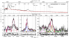 |
Fig. A.1. Top panel: calibrated rest-frame spectrum of SDSS000807.27-103942.7 before continuum substraction. Abscissa is rest-frame wavelength in Å, while ordinate is specific flux in units 10−15 erg s−1 cm−2 Hz−1. Global or local continuum are specified by a continuous line. Dot-dashed vertical lines identify the position at rest-frame of the strongest emission lines. Bottom panel: multicomponent fits after continuum subtraction for the Si IV |


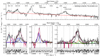 |
Fig. A.10. Same as Fig. A.1, for SDSSJ125659.79-033813.8. |
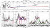 |
Fig. A.11. Same as Fig. A.1, for SDSSJ131132.92+052751.2. |
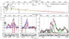 |
Fig. A.12. Same as Fig. A.1, for SDSSJ143525.31+400112.2. |
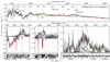 |
Fig. A.13. Same as Fig. A.1, for SDSSJ144412.37+582636.9. |
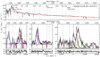 |
Fig. A.14. Same as Fig. A.1, for SDSSJ151258.36+352533.2. |
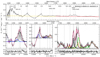 |
Fig. A.15. Same as Fig. A.1, for SDSSJ214009.01-064403.9. |
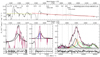 |
Fig. A.16. Same as Fig. A.1, for SDSSJ220119.62-083911.6. |
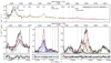 |
Fig. A.17. Same as Fig. A.1, for SDSSJ222753.07-092951.7. |
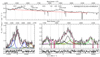 |
Fig. A.18. Same as Fig. A.1, for SDSSJ233132.83+010620.9. |
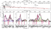 |
Fig. A.19. Same as Fig. A.1, for SDSSJ234657.25+145736.0 |
Appendix B:
Error estimates
Emission lines of the xA spectra are blended in almost all cases. For example, in the 1900 Å blend the emission of C III] 1909 and Fe IIIλ1914 cannot be deblended; or in the case of C IV the separation between broad and blue components is not obvious.We built Monte Carlo (MC) simulations to determine the error estimates, in order to consider the effects of blending. The MC method allows us to consider all emission components and include a variation of the flux and FWHM simultaneously. The method is based on minimizing the χ2 (Barlow 1989). A variation in parameters of the line properties causes changes in the χ2. Then, the parameters at 1σ confidence level are those that satisfy the constraint:
  (Andrae 2010).
The MC method is applied to the same spectral regions identified for the multicomponent fits with SPECFIT (Sect. 4.2). All line components considered in modeling the observed quasar emission spectrum were taken into account. For example, in the 1900 Å blend region variations in flux and FWHM of Al III, Si III], C III], Si II 1816, N III]
 1750, Fe II and Fe III are considered for each simulation. Parameters vary around the values given by the SPECFIT model without any constraint and the simulations are therefore totally independent of the SPECFIT model.
We ran 5000 simulations for each quasar in order to obtain good sampling. Left panels of Fig. B.1 show the distributions of χ2 for the flux of Al III (top) and for the total C IV profile (bottom), for the quasar SDSSJ222753.07-092951.7. Usually ∼1000–3000 simulations satisfy the criterion  . The total width of the distribution at
  is the 1σ error confidence level we consider for each parameter. The central panels of Fig. B.1 show the 1900 Å blend (top) and C IV (bottom) spectra, and the quasar emission associated with the 1σ confidence level derived from the MC simulations (gray shadow regions).
Strongest emission lines like Al III or the total emission of C IV show Gaussian distributions for the flux and FWHM MC replications (see right panels of Fig. B.1). However, for weak lines like C III] 1909, N III]
 1750 or He II
 1640BC, the distribution has an asymmetric or flat behavior. This is because faint lines are strongly affected by the presence of the stronger ones (e.g., Si II
 1816 affected by Al III). In these cases, we consider the flux found by SPECFIT as an upper limit. We report the FWHM values followed by a double colon to signify a high uncertain value (Tables 4–7).
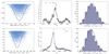 |
Fig. B.1. Left panels: distribution of χ2 as a function of the flux of Al III (top) and total C IV profile (bottom). Black continuous lines mark the normal distribution associated with simulations. Gray horizontal lines indicate the value at |


Appendix C:
FeII and FeIII
C.1 Identification of Fe and Fe transitions
In next lines are described the most important Fe II and Fe III transitions in the spectral range 1700–2100 Å. Table reports the approximate central wavelength of the Fe II and Fe III features, the multiplet identification, and the sources where they are prominent.
Fe II
-
[λ1715 Å] – This feature has not been identified previously as Fe II emission. Graham et al. (1996) suggest Al II associated with the 3p3Po − 3d3D transitions. However, the wavelength consistency is poor, the Al II transition is fairly high level, and its intensity is predicted negligible even for very low ionization parameter (∼10−3). We therefore ascribe the feature to Fe II UV multiplet #38 (associated with the transition between terms a4F−4Do), and specifically to the transition
 that has the higher oscillator strength among all Fe II lines listed by Kurucz & Bell (1995) loggf ≈ −0.395.
 -
[λ1785 Å] – The UV multiplet #191 is strong in several quasars, most notably I Zw 1 (Marziani et al. 1996; Laor et al. 1997; Vestergaard & Wilkes 2001). The emission is believed to be enhanced by a Ly
 fluorescence mechanism (Baldwin et al. 2004) also operating in symbiotic stars and in stars with chromospheric activity (Johansson & Hansen 1988; Johansson et al. 1995).
 -
[λ2020 Å] – This feature is never strong (≲2 Å), but is apparently detected in a few objects (Table ). The main feature could be associated with the line at 2020.739 Å and other two lines of Fe II multiplet UV #83.
-
[λ1914 Å] – The line of the Fe III UV multiplet #34 is included in the template. We added a component to take into account the possibility of extraordinary enhancement due to Ly
 fluorescence, as outlined in Marziani et al. (2010).
 -
[λ2005 Å & λ2045 Å] – These features have been identified as due to Fe III UV #55 (Graham et al. 1996; Vestergaard & Wilkes 2001).
-
[λ2080 Å] – This feature is perhaps the most prominent one among the Fe III features. Its identification Fe III UV #48 is supported by the consistency in wavelength of the three multiplet components. The peculiarity of the GTC-xA sources is that the feature is not reproduced well by the template: an additional component is needed. The analysis of the 2080 Å feature is reported in Sect. 6.4, and its origin is discussed in Appendix C.2 below.
-
[λ2093 Å] – We identify this feature as due to Fe III UV #77 (Vestergaard & Wilkes 2001). A previous identification as Fe I seems less likely, considering that Fe I features are predicted to be exceedingly weak (Sigut et al. 2004) even at the lowest ionization degrees.
-
[λ2115 Å] – Vestergaard & Wilkes (2001) associates this feature with Fe III UV #58.
C.2 On the origin of Fe III emission
The strength of Fe III emission is surprising, given that the overall appearance of the spectrum is suggestive of extremely low ionization. The Fe III features have also been observed in Pop. A sources or associated with extreme Pop. A (e.g., (Baldwin et al. 1996; Graham et al. 1996; Richards et al. 2011)). The Fe III lines
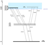 |
Fig. C.1. Partial Grotrian diagram showing the energy levels and the spectroscopic terms associated with the emission of Fe III multiplet #48, #118 (top left) and #119 (top right). Energy level separation is not drawn to scale for clarity. |
Identification of Fe II and Fe III features.
are mainly emitted in a region at the boundary between the fully and partially ionized zone. At ionization parameter logU ≳ −2, the region of Fe III line formation is usually a region where the opacity in the Lyman continuum grows to values τ912 ≳ 1 (i.e., a small fraction of the geometric depth of the emitting gas of slab). Deeper into the slab from its illuminated face, the dominant ionization stage is Fe+3. A significant fraction of Fe III is present at the illuminated face of the cloud within the H II zone, but only if the ionization parameter is very low (logU ≲ −3, Fig. 3 of Sigut et al. 2004). Fe+2 is ≲2% of Fe+1 in the partially-ionized zone (PIZ): Fe+1 still remains the dominant ionization stage of iron in the PIZ, as required by the strong optical Fe II emission required for these sources. In the spectral range between 1800 and 2100 Å, however, the dominant contribution may be due to Fe III, as predicted by the models of Sigut et al. (2004), which assumes logU ∼ −3.
The role of Ly fluorescence in explaining the UV and IR Fe II emission has been known since the late 1980s from photoionization simulations (e.g., (Sigut & Pradhan 1998; Verner et al. 2004; Sigut et al. 2004)) as well as from observational evidence (e.g., (Penston 1987; Marinello et al. 2016; Clowes et al. 2016) and references therein). As mentioned, a specific feature that is believed to be enhanced by Ly
 fluorescence is the Fe IIUV #191 multiplet at 1785 Å. Also the Fe III line at λ1914, ascribed to the transition of the Fe IIUV #34 multiplet z
 a7S3, is expected to be enhanced by Ly
 fluorescence. Although this is not a resonant line (the lower level is ∼3 eV above ground), the line appears often stronger than in the Vestergaard & Wilkes (2001) template, presumably because the upper level is populated by Ly
 fluorescence (Marziani et al. 2010). Figure 8 suggest a close association between the 2080 feature and the Fe II and Fe III features enhanced by Ly
 fluorescence.
Generally speaking, we expect that Ly fluorescence may be also relevant in the explanation of the overall Fe III spectrum, considering the large number of radiative transitions possible for the electronic configuration of the Fe++. The Fe III high ionic fraction in the H II zone and at the transition zone between H II and PIZ are expected to be conditions that make the fluorescent absorption of Lyman continuum photons by Fe III ions especially efficient. In the specific case of the 2080 feature, we suggest that a mechanism of enhancement is due to fluorescence with the Lyman continuum ionization edge. The Fe III UV #48 multiplet is radiatively linked to the multiplets #118 and #119 between the terms z5Po e5D and e5S, respectively. The energy difference between the lower level of the lower a5S term of multiplet #48 and the upper terms of #118 and 119, is 13.65 and 13.67 eV, respectively, slightly above the ionization potential of hydrogen (13.5984 eV). Figure schematically shows the energy levels associated with the spectroscopic terms. Even if the energy is not strictly coincident, the Lyman continuum emission (which is expected to decrease with ν−3) may act as a broadened pseudo-line.
If this mechanism is indeed operating, we expect Fe III emission from multiplets UV #118 and #119 in the range 1595–1610 Å. A faint hump present on the composite spectrum in the predicted range could be due to some Fe III emission as well as to the blueshifted component of He II 1640 blending with the red side of C IV
 1549. Considering the weakness of the features, and the severe blending with He II
 1640 and C IV
 1549, the prediction of Fe III emission around 1600 Å should be verified on high S/N spectra of sources with narrower lines.
All Tables
All Figures
|
Fig. 1. Top panel: rest-frame composite spectrum (see Sect. 5.1). Abscissa corresponds to vacuum rest-frame wavelength in Å, while ordinate is in arbitrary intensity. Dot-dashed vertical lines identify the position at rest-frame of the strongest emission lines. Bottom panels: multicomponent fits after continuum subtraction for the 1400 Å blend, C IV |
| In the text | |
|
Fig. 2. Relation between intensity ratios Al IIIλ1860/Si III |
| In the text | |
|
Fig. 3. Relation between the |
| In the text | |
|
Fig. 4. Relation between the FWHM Alλ1860 and FWHM C |
| In the text | |
|
Fig. 5. Rest-frame equivalent width distributions of the Al IIIλ1860, Si III |
| In the text | |
|
Fig. 6. From top to bottom, rest-frame composite spectra of the GTC-xA, FOS-xA, and S14-A. Intensity units are arbitrary flux. The GTC-xA and FOS-xA have been displaced by a constant value for clarity. |
| In the text | |
|
Fig. 7. Isocontours in the plane log of ionization parameter (U) versus log of hydrogen density ( |
| In the text | |
|
Fig. 8. Relation between intensity of the Fe III feature at 2080 Å with Fe UV 1785 Å (blue) and Fe IIIλ1914 (red). Squares, up and down triangles, and circles mark the normal, BAL, mini–BAL and RL quasars, respectively. The gray shaded area indicates an approximate detection limit. Blue and red lines mark the orthogonal fit for each case. |
| In the text | |
|
Fig. 9. Behavior of the centroid at 1/2 of total C |
| In the text | |
|
Fig. 10. Relation between rest-frame equivalent width of C IV |
| In the text | |
|
Fig. A.1. Top panel: calibrated rest-frame spectrum of SDSS000807.27-103942.7 before continuum substraction. Abscissa is rest-frame wavelength in Å, while ordinate is specific flux in units 10−15 erg s−1 cm−2 Hz−1. Global or local continuum are specified by a continuous line. Dot-dashed vertical lines identify the position at rest-frame of the strongest emission lines. Bottom panel: multicomponent fits after continuum subtraction for the Si IV |
| In the text | |
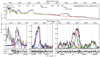 |
Fig. A.2. Same as Fig. A.1, for SDSSJ004241.95+002213.9. |
| In the text | |
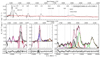 |
Fig. A.3. Same as Fig. A.1, for SDSSJ021606.41+011509.5. |
| In the text | |
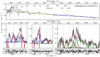 |
Fig. A.4. Same as Fig. A.1, for SDSSJ024154.42-004757.5. |
| In the text | |
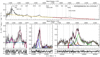 |
Fig. A.5. Same as Fig. A.1, for SDSSJ084036.16+235524.7. |
| In the text | |
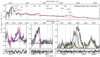 |
Fig. A.6. Same as Fig. A.1, for SDSSJ101822.96+203558.6. |
| In the text | |
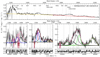 |
Fig. A.7. Same as Fig. A.1, for SDSSJ103527.40+445435.6. |
| In the text | |
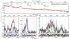 |
Fig. A.8. Same as Fig. A.1, for SDSSJ105806.16+600826.9. |
| In the text | |
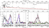 |
Fig. A.9. Same as Fig. A.1, for SDSSJ110022.53+484012.6. |
| In the text | |
|
Fig. A.10. Same as Fig. A.1, for SDSSJ125659.79-033813.8. |
| In the text | |
|
Fig. A.11. Same as Fig. A.1, for SDSSJ131132.92+052751.2. |
| In the text | |
|
Fig. A.12. Same as Fig. A.1, for SDSSJ143525.31+400112.2. |
| In the text | |
|
Fig. A.13. Same as Fig. A.1, for SDSSJ144412.37+582636.9. |
| In the text | |
|
Fig. A.14. Same as Fig. A.1, for SDSSJ151258.36+352533.2. |
| In the text | |
|
Fig. A.15. Same as Fig. A.1, for SDSSJ214009.01-064403.9. |
| In the text | |
|
Fig. A.16. Same as Fig. A.1, for SDSSJ220119.62-083911.6. |
| In the text | |
|
Fig. A.17. Same as Fig. A.1, for SDSSJ222753.07-092951.7. |
| In the text | |
|
Fig. A.18. Same as Fig. A.1, for SDSSJ233132.83+010620.9. |
| In the text | |
|
Fig. A.19. Same as Fig. A.1, for SDSSJ234657.25+145736.0 |
| In the text | |
|
Fig. B.1. Left panels: distribution of χ2 as a function of the flux of Al III (top) and total C IV profile (bottom). Black continuous lines mark the normal distribution associated with simulations. Gray horizontal lines indicate the value at |
| In the text | |
|
Fig. C.1. Partial Grotrian diagram showing the energy levels and the spectroscopic terms associated with the emission of Fe III multiplet #48, #118 (top left) and #119 (top right). Energy level separation is not drawn to scale for clarity. |
| In the text | |
Current usage metrics show cumulative count of Article Views (full-text article views including HTML views, PDF and ePub downloads, according to the available data) and Abstracts Views on Vision4Press platform.
Data correspond to usage on the plateform after 2015. The current usage metrics is available 48-96 hours after online publication and is updated daily on week days.
Initial download of the metrics may take a while.