| Issue |
A&A
Volume 618, October 2018
|
|
|---|---|---|
| Article Number | A79 | |
| Number of page(s) | 18 | |
| Section | Stellar structure and evolution | |
| DOI | https://doi.org/10.1051/0004-6361/201833401 | |
| Published online | 16 October 2018 | |
Insights into the inner regions of the FU Orionis disc⋆
1
Mount Suhora Observatory, Krakow Pedagogical University, ul. Podchorazych 2, 30-084 Krakow, Poland
e-mail: This email address is being protected from spambots. You need JavaScript enabled to view it.
2
Astronomical Observatory, Jagiellonian University, ul. Orla 171, 30-244 Krakow, Poland
3
Département de Physique, Université de Montréal, CP 6128, Succursale: Centre-Ville, Montréal, QC, H3C 3J7, Canada
4
Department of Astronomy and Astrophysics, University of Toronto, 50 George St., Toronto, Ontario, M5S 3H4, Canada
5
Department of Mathematics, Physics & Geology, Cape Breton University, 1250 Grand Lake Road, Sydney, NS, B1P 6L2, Canada
6
Canadian Coast Guard College, Dept. of Arts, Sciences, and Languages, Sydney, Nova Scotia, B1R 2J6, Canada
7
Department of Physics & Astronomy, University of British Columbia, 6224 Agricultural Rd, Vancouver, BC, V6T 1Z1, Canada
8
Universität Wien, Institut für Astrophysik, Türkenschanzstrasse 17, 1180
Wien, Austria
9
Institute for Computational Astrophysics, Department of Astronomy and Physics, Saint Marys University, Halifax, NS, B3H 3C3, Canada
10
Harvard-Smithsonian Center for Astrophysics, 60 Garden Street, Cambridge, MA, 02138, USA
Received:
9
May
2018
Accepted:
4
July
2018
Abstract
Context. We investigate small-amplitude light variations in FU Ori occurring in timescales of days and weeks.
Aims. We seek to determine the mechanisms that lead to these light changes.
Methods. The visual light curve of FU Ori gathered by the MOST satellite continuously for 55 d in the 2013–2014 winter season and simultaneously obtained ground-based multi-colour data were compared with the results from a disc and star light synthesis model.
Results. Hotspots on the star are not responsible for the majority of observed light variations. Instead, we found that the long periodic family of 10.5–11.4 d (presumably) quasi-periods showing light variations up to 0.07 mag may arise owing to the rotational revolution of disc inhomogeneities located between 16 and 20 R⊙. The same distance is obtained by assuming that these light variations arise because of a purely Keplerian revolution of these inhomogeneities for a stellar mass of 0.7 M⊙. The short-periodic (∼3 – 1.38 d) small amplitude (∼0.01 mag) light variations show a clear sign of period shortening, similar to what was discovered in the first MOST observations of FU Ori. Our data indicate that these short-periodic oscillations may arise because of changing visibility of plasma tongues (not included in our model), revolving in the magnetospheric gap and/or likely related hotspots as well.
Conclusions. Results obtained for the long-periodic 10–11 d family of light variations appear to be roughly in line with the colour-period relation, which assumes that longer periods are produced by more external and cooler parts of the disc. Coordinated observations in a broad spectral range are still necessary to fully understand the nature of the short-periodic 1–3 d family of light variations and their period changes.
Key words: accretion, accretion disks / stars: individual: FU Ori / stars: pre-main sequence
Tables A.1–A.21 are only available at the CDS via anonymous ftp to cdsarc.u-strasbg.fr (130.79.128.5) or via http://cdsarc.u-strasbg.fr/viz-bin/qcat?J/A+A/618/A79
© ESO 2018
1. Introduction
FU Orioni-type stars (FUors) were already recognised as classical T Tauri-type stars (CTTS) undergoing a phase of enhanced disc brightness by Herbig (1977). The light outburst is due to an increased mass accretion rate from 10−11 − 10−7M⊙ yr−1 typical in CTTS, up to 10−5 − 10−4M⊙ yr−1 in FUors (Hartmann & Kenyon 1985, 1996). During the FUor phase, the emission-line rich visual spectrum of the formerly quiet CTTS is dominated by the absorption features produced in the inner accretion disc. Its inner parts radiate as the photosphere of an F-G supergiant star, while the slightly colder and more distant parts of the disc produce a K-M type supergiant spectrum that can be observed in the near-infrared (Kenyon et al. 1988). In these circumstances disc radiation dominates stellar radiation (usually an early-M or late-K dwarf) by 100–1000 times. This makes FUors well suited for inner disc variability studies in visual bands in early stages of star formation, presumably during the first 0.3 Myr of evolution when discs are gravitationally unstable (Hartmann 1998; Liu et al. 2016).
In 1937, FU Ori , which is the prototype of FUors, increased its brightness from 15.5 ± 0.5 to 9.7 ± 0.1 mag (Clarke et al. 2005) in the photographic system, whose effective wavelength λ is similar to that of the Johnson B filter. The star still remains in a high state of brightness with only 1.3 mag decrease noticed until 2014 in the B filter (see Sect. 2.3). Our target was briefly described in our first paper of this series (Siwak et al. 2013) and also in Powell et al. (2012) and Audard et al. (2014); the latter authors presented a detailed review regarding eruptive young stars, both FUors and EX Lupi-type stars (EXors), emerging from observations obtained in a broad spectral range.
Most of the photometric and spectroscopic historical papers concern the variability of FU Ori occurring on timescales of months to years (see e.g. Clarke et al. 2005). In the pre-space telescope era nightly breaks and non-uniform weather patterns imposed severe limitations on light variability studies on a daily scale, occurring on top of the light plateau caused by enhanced accretion. The most in-depth though indirect study of this subject was made by Kenyon et al. (2000). After a careful consideration of several hypotheses the authors concluded that the disc likely shows flickering, occurring with a characteristic timescale of predominantly about one day, and that variations of the colour indices obtained in the Johnson filters point to the region extending between the stellar photosphere and the radius where the disc temperature reaches its maximum as the dominant source of the variability. We note that Kolotilov & Petrov (1985) and Ibragimov (1993) were also unable to find any stable periods in the data sets gathered during the 1980s. Instead the authors found quasi-periodic oscillations (QPOs) that appeared to evolve from 18.35 to 9.19 d in the course of the single 1984–1985 observing season. The 9.2 d QPO was also visible during 1987–1988 along with possible 9.8 and 11.4 d QPOs.
Having the advantage of contiguous monitoring of stars for a few weeks from space with the MOST satellite and with such photometric precision unavailable from the ground, we decided to use this space telescope for a direct search and characterisation of short-period, small-amplitude light variations in FU Ori during winter 2010–2011. Our first results (Siwak et al. 2013) can be summarised as follows:
The light curve itself and its Fourier and wavelet transform spectra reveal two major QPOs. The first has a larger amplitude and possibly changes its period in the range 8–9 d. The second, of a smaller amplitude, is apparently time coherent, and was initially observed at about 2.4 d, but drifted down to 2.2 d, well before the end of the run. The longer variation was less securely defined in the 28-day-long run to conclude that this was really a time-coherent QPO. Light changes occurring on the timescale of ≤1 d, predicted by the Monte Carlo model of Kenyon et al. (2000) to dominate in the light curve, were observed in the light curve for a very limited time only. Moreover, Zhu et al. (2007) investigated the spectral energy distribution in FU Ori and argued against the putative boundary layer extending towards the stellar photosphere (see Sect. 5.1 of their paper), i.e. the “energy release zone” (Luybarskii 1997) proposed to be responsible for the disc flickering by Kenyon et al. (2000). In these circumstances, assuming a stellar mass of 0.3 M⊙ (Zhu et al. 2007), we indisputably interpreted that variations observed by MOST were produced by the hot plasma condensations that develop in the magneto-rotationally unstable inner parts of the disc at distances of about 12 and 5 R⊙, respectively. The period shortening may be interpreted as spiralling-in or inward drifts in the inner disc. Assuming Keplerian rotation of the disc, we also temporarily proposed that the shortest observed period of 2.2 ± 0.1 d may define the inner edge of the disc at 4.8 ± 0.2 R⊙, which agrees with the  R⊙ result from the interferometric observations of Malbet et al. (2005).
Our two-colour Strömgren v and b filter ground-based observations of FU Ori at the Mount Suhora Observatory (MSO) substantially confirmed the (B − V) versus V relation obtained by Kenyon et al. (2000). However, we obtained a slightly redder colour index of the dominant 8 d variation, which we tentatively interpreted as due to a more outward location of the inhomogeneity causing this quasi-periodicity. This would agree with the interpretation of the colour-period relationship through different locations of the dominant variable flux with longer periods produced by more external and cooler parts of the disc. We decided to examine this relationship based on new MOST data collected as long as technically possible, and simultaneously obtained multi-colour observations from the ground during the 2013–2014 observing season.
We describe the MOST satellite and ground-based multi-colour observations of FU Ori obtained at the MSO and at the South African Astronomical Observatory (SAAO) in Sect. 2. Results from the data analyses are presented in Sect. 3. We discuss the obtained results in the context of recent theories proposed for CTTS and FUors in Sect. 4 and summarise in Sect. 5.
2. Observations
2.1. MOST observations
The pre-launch characteristics of the MOST satellite mission are described in Walker et al. (2003) and the initial post-launch performance in Matthews et al. (2004). The satellite observes in one broadband filter covering the spectral range from 370 nm to 750 nm with effective wavelength similar to that of the Johnson V filter.
The observations of FU Ori were made in the direct imaging data acquisition mode of the satellite. A run of length 54.93 d started on November 20, 2013 and lasted until January 15, 2014 (HJD = 2456616.5408–2456671.4662). Because of the slow temporal changes in the light curve noticed during the first MOST run in 2010–2011, and to permit alternate, multi-object observations, the star was observed during every second satellite orbit, i.e. with a typical cadence of 202.87 min. The individual exposures were 60 s long and typically ten to a few dozen exposures per orbit were obtained. The photometry (Fig. 1a and Table A.1) was extracted from the raw data and de-correlated with known instrumental effects using the dedicated pipeline introduced by Rowe et al. (2006). In spite of this advanced process, a significant systematic trend is visible in the primary and secondary targets; this trend is possibly owing to changing sensitivity of the electronic system. This affected all stars observed in the field, but affected each star in a slightly different way, preventing their use in removing the FU Ori light-curve trend. To eliminate the problem, we used our BVRcRIcI filter data for FU Ori obtained simultaneously at the SAAO and MSO (see in Fig. 1b, and next two Sections for details). In this process, the U-filter data had to be abandoned owing to their significantly higher scatter. The eight-degree polynomial fitted to the differences between the MOST and the BVRcRIcI averaged data (matching the bandwidth of the MOST satellite) was then subtracted from the MOST pipeline result giving variations as shown in Fig. 1c (Table A.2); the magnitude level is arbitrary in this panel. Finally, we calculated mean-orbital data points, as shown in Fig. 1d (Table A.3). Their median error (σ) is 0.0019 mag in the full range 0.0002–0.0078 mag. One can notice a few major gaps in the data acquisition at HJD-2 456 500 = 138.5–139.6, 142.4–143.5, 149.7–150.6, 158.5–159.9, 162.4–163.1 and 163.4–164.4 owing to observations of other, time-critical targets. These gaps were short in comparison to the variability timescales observed in this star and do not affect our conclusions.
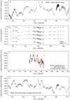 |
Fig. 1. First panel: 2013–2014 MOST light curve of FU Ori provided by the pipeline. The standardised SAAO UBVRcIc (filled circles) and aligned MSO BVRI light curves (open circles and crosses) are shown in the second panel. Third panel: averaged SAAO BVRcIc (filled circles) and MSO BVRI (open circles) observations used for correction of the instrumental trend in the original MOST data, as described in Sect. 2.1. The de-trended MOST data are plotted in the same panel. Fourth panel: de-trended MOST data in the form of orbital averages with error bars (σ). |
2.2. Observations by MSO uvyBVRI filters
In order to search for long-period light variations, which is not possible using MOST because of the technical limitation of a single run to about 55 d, we conducted time variability monitoring of FU Ori at the MSO. We started our observations on September 3, 2013, and continued the monitoring for 220 d, i.e. until April 11, 2014, when the altitude of the star amounted to only 30 deg at civil dusk. During this interval, useful data were obtained on 69 nights, out of which 20 coincided with the satellite run.
We used three different photometric systems on the 0.6 m telescope. During the first five nights of September, we used a SBIG ST10XME CCD camera equipped with the Johnson-Morgan BVRI filters provided by SBIG. The data obtained with this instrument are indicated as crosses in Fig. 1b. On September 30, 2013, the Apogee Alta U42 CCD camera, equipped with a different set of wide band BVRI Johnson (Bessell) filters manufactured by Custom Scientific, was installed on the telescope and the data are indicated by open circles. We decided to use only this uniform data set for further analyses, which limited the monitoring time to 194 d. Additionally, for 24 nights between November 12, 2013 and January 13, 2014 (18 nights during the MOST run), we observed the star with Strömgren uvy filters.
On each clear night typically 10–30 single exposures per filter for FU Ori were obtained. All frames were dark and flat-field calibrated in a standard way within the MIDAS package (Warmels 1991). The correction for bias was accomplished using the same exposure for dark as for science frames. The photometric data were extracted using the C-MUNIPACK programme (Motl 2011) using the DAOPHOT II package (Stetson 1987). A constant aperture of 12 pixels (corresponding to 13.44 arcsec on the sky for a scale of 1.12 arcsec per pixel) was used for FU Ori and the comparison stars. To avoid possible errors associated with the arc-like nebula surrounding FU Ori, relatively large annuli (from 20 to 30 pixels, i.e. 20 to 34 arcsec) were used for the sky background calculations.
The differential photometry used a mean comparison star that was formed from two stars (Table 1), following Siwak et al. (2013), both apparently stable to about 0.01 mag in all filters throughout the entire MSO run. We corrected our data for dominant colour extinction effects using the mean coefficients for this site. Since FU Ori turned out to be essentially constant during nightly monitoring sessions of about 20–30 min, nightly averages were calculated. The data obtained in Johnson filters were later manually aligned with the BVRcIc standardised SAAO light curves (see in Fig. 1b, and also in Table A.4–A.7). The data obtained in Strömgren filters were left in the instrumental system (Tables A.8–A.10).
2.3. Observations by SAAO UBVRcIc filters
FU Ori was observed at the SAAO on 25 nights from December 5, 2013 to January 14, 2014 using the 0.5 m Boller & Chivens telescope equipped with well-known for its reliability single-channel Modular Photometer. This photometer was equipped with a Hamamatsu R943-02 GaAs photomultiplier and a set of UBVRcIc Johnson–Cousins filters (see in Fig. 1b). For all observations, a 25 arcsec aperture was utilised; thereby a part of the associated arc-like nebulae light (however, negligibly small) was also recorded. The differential photometry of FU Ori utilised the same two comparison stars as those used at the MSO (Table 1). Performing all-sky absolute photometry, commonly practised at the SAAO with this instrument, was impossible owing to a large number of not fully photometric nights during the first two weeks of the run. We measured the target (var), comparison stars (comp1, comp2), and sky background (sky) in the sequence of sky-comp1-comp2-sky-var-sky-comp2-comp1-sky-comp2-comp1-sky-var-sky-comp1-comp2-sky, repeated two or three times. During the moonless nights (except for those with a high airglow activity) the sky sampling rate was reduced since the background level remained stable for about an hour. The rate of sky monitoring was considerably increased during the rising and setting of the Moon. The two full Moon passages through the field during the run forced us to discard observations of FU Ori during that time owing to strong background gradients, especially in the UB filters, and to rely entirely on simultaneous CCD observations at the MSO, which have the advantage that the sky level is individually calculated from pixels surrounding each star.
Colour equation coefficients determined for the SAAO UBVRcIc system during the night of January 11–12, 2014.
2.3.1. Determination of colour equations for the SAAO system
We observed a set of eight standard stars from the E400 region (Menzies et al. 1989) in the night of January 11–12, 2014, in excellent photometric conditions. Transformation equations to standard magnitudes  for each filter ft ∈ {U, B, V, Rc, Ic} took the following form:
 (1)
(1)
where  is the observed (instrumental) magnitude calculated from the dead-time and sky-level corrected counts, kft is the mean SAAO differential extinction, βft is the colour extinction evaluated for SAAO from Fukugita et al. (1996) and Mt. Palomar sites, μft is the system transformation coefficient, the constant Cft is the zero point in magnitude, and CI is the colour index defined as the magnitude difference of neighbouring filters. We present the obtained values and respective CI terms for every filter in Table 2, while the resulting magnitudes of the comparison stars are given in Table 1. This enabled the absolute calibration of the FU Ori UBVRcIc light curves, as show in Fig. 1b (Tables A.11–A.15). We did not derive colour equations for the MSO system; instead, the BVRI light curves were aligned to the SAAO BVRcIc data, using observations obtained simultaneously at both observatories (Tables A.4–A.7). We estimate the accuracy of this procedure to be about 0.002 mag.
2.3.2. Determination of colour indices from the SAAO data
Using single channel photometry, colour indices can be calculated in two ways: first, through subtraction of the two light curves obtained with the use of comparison stars (as for the MSO data); or second, using the variable star only, relating its sky- and dead-time-corrected measurements in two colours and using colour equations determined above in Sect. 2.3.1. The first method involved too large scatter into the final results owing to the accumulation of noise from the comparison stars. This is particularly the case when these stars are fainter than the target and the sequence of measurements given in Sect. 2.3 was not executed in the fully photometric conditions that prevailed during the first two weeks of our run. For that reason, we calculated the colour indices using the second method. For example, to obtain V − Ic colour indices, the flux ratios between the V-filter data points and the reference 1–3 deg polynomial (obtained from a fit to Ic-filter points) were transformed to the magnitude scale, corrected for differential and colour extinctions, and then transformed to the standard system using Eq. (1) and coefficients listed in Table 2. We plot the final results in Fig. 2 and show in electronic form in Tables A.16–A.20.
2.4. Spectroscopic SAAO observations
In the evening of March 11, 2017, we obtained a few low-resolution spectra of FU Ori at the SAAO using the SpUpNIC – Spectrograph Upgrade-Newly Improved Cassegrain (Crause et al. 2016), mounted on the 1.9 m Radcliffe telescope. Grating 6 was used to cover the wavelength range from 3904 Å to 6650 Å with a resolution of 1.35 Å pixel−1. Two spectroscopic standard stars LTT 2415 and LTT 3864 were observed immediately after our target using the same slit width of 3.59 arcsec. The spectra were extracted and then wavelength- and flux-calibrated within the IRAF package. Only these FU Ori and standard-star spectra, for which no telescope-guiding errors were noticed during the 120 s-long integrations, were selected for further analyses.
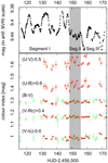 |
Fig. 2. New MOST light curve of FU Ori (top panel) and the ground-based U − V, U − B, B − V, V − Rc and V − Ic colour indices (lower panel) in standard magnitudes, with arbitrary offsets indicated. As mentioned in the text, the MSO data (open circles) were aligned to the standardised SAAO data (filled circles) with an accuracy of 0.002 mag. The grey-shaded area determines the approximate boundaries of Segment II data, as defined in Sect. 3. The Segment I data are shown on the left, while the Segment III data are shown on the right. |
3. Results of data analysis
3.1. General description of variability
The 2013–2014 MOST light curve (Fig. 1d) appears to consist of three segments, each defined by a characteristic pattern of the FU Ori variability. These patterns exist for some time and then disappear. The three segments, indicated in Fig. 2, have the following characteristics:
-
1.
We define as Segment I the part from the beginning of the MOST observations (at least) until HJD ≈ 2 456 647.8, which is dominated by consecutive peaks of different heights, i.e. 0.07 and 0.02 mag. Careful insight into the ground-based averaged data (Fig 1c) reveals that this variability pattern began in fact about 20 d earlier, at HJD ≈ 2 456 595, with the appearance of the broad local light maximum. The ground-based data also suggest that the height of the maximum observed by MOST as the smaller one (i.e. of 0.02 mag), could initially be higher. This variability pattern is very similar to what was observed by MOST in IM Lupi, which is visible at an inclination angle of 60 deg and where two stable polar hotspots played a major role in the observed light modulations (Siwak et al. 2016). This conclusion was inferred by utilising the numerical results of Romanova et al. (2004) and Kulkarni & Romanova (2008) for stars accreting in a stable regime, which more likely is the case for CTTS with low accretion rates. We note that stable polar hotspots were also found in EX Lupi (the prototype of EXors) during a quiescent phase using spectroscopic data (Sicilia-Aguilar et al. 2015). For geometrical reasons one may think that the same mechanism operates in FU Ori, which most likely is observed at an inclination of 55° (Malbet et al. 2005). Additionally, the characteristic re-appearance time for the observed peaks, both larger (∼0.07 mag) and smaller (∼0.02 mag) appears to be about 10–11 d, which is of the same order as the 7.2–7.6 d rotational period of IM Lupi, and 7.41 d in EX Lupi (Sipos et al. 2009). However, despite large observational errors, the U − V, U − B and B − V colour indices appear to be systematically slightly redder when the star is brighter, while the V − Rc and V − Ic light curves appear to be stable, as shown in Fig. 2 for the Segment I data. This seems to contradict the hotspot hypothesis and we return to this issue later in this paper. We note that the last maximum in Segment I centred at HJD-2 456 500 ≈ 146 is double-peaked. Starting from this place the present light variability pattern appears to smoothly transform into the next, which is defined below.
-
2.
Segment II of the light curve consists of small-amplitude sine-like variations, showing a period shortening of each successive oscillation. It is indicated by a grey-shaded area in Fig. 2. The sine-like wave lasted for at least eight days and ceased at HJD-2 456 500 ≈ 156 when its initial period of about 3 d shortened to 1.38 ± 0.04 d. The colour indices appear to be stable but this is not a very significant statement given the small 0.005–0.01 mag amplitude of these oscillations, which is comparable to the measurement errors of the ground-based data.
-
3.
Segment III of the light curve begins after HJD-2 456 500 ≈ 156, when the star brightness started to drop by about 0.05 mag (until the first minimum at HJD-2 456 500 ≈ 158.1) and then it rose by 0.06–0.07 mag in the MOST magnitude system. The symmetry of these light changes and a second, similar event at HJD-2 456 500 ≈ 169.5, appearing 11.4 d after the first, suggest their similar origin. Unfortunately, the MOST monitoring finished soon after the second deep light minimum event owing to technical limitations on the satellite run length. Furthermore, termination of our SAAO run and poor weather conditions over the MSO at the same time, shortened the photometric monitoring of this feature from the ground. Therefore, the question of whether we observed an initiation of a new QPO remains open. Its putative 11.4 d period might suggest the same physical mechanism that operated during Segment I, especially that also a secondary light drop occurred at HJD-2 456 500 ≈ 163. Interestingly, all but the U − V and U − B colour indices in Segment III appear to be stable during the first deep minimum, but during the second, at HJD-2 456 500 ≈ 169.5, two slightly redder points in the V − Rc and V − Ic light curves were found in the SAAO data.
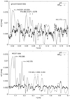 |
Fig. 3. Results of Fourier analysis of ground-based (upper panel) and MOST (lower panel) data in form of the amplitude a(f) vs. the frequency (f) are shown as continuous lines. The amplitude errors, determined from bootstrap sampling, are shown as dots. |
3.2. Frequency analysis of the FU Ori data
We performed frequency analyses of two data sets: the first utilised the long-term MSO BVRI and SAAO BVRcIc nightly-averaged data points, i.e. those that were previously used as a fiducial comparison star for the MOST data trend removal; the second utilised the MOST mean-orbital data points.
We used the procedure previously developed by Rucinski et al. (2008). The Fourier analysis was done by consecutive, in the frequency f space with a step of Δf = 0.001, least-squares fits of expressions of the form l(f)=c0(f)+c1(f) cos[2π(t − t0)f]+c2(f) sin[2π(t − t0)f]. The amplitude a(f) for each frequency was found as the modulus of the periodic component,  . The bootstrap sampling technique permitted evaluation of mean standard errors of the amplitudes from the spread of the coefficients ai.
The Fourier spectra of ground-based data (the upper panel in Fig. 3) shows two families of peaks above the noise level (of about 0.007 mag) in the ranges f = 0.021 − 0.024 c d−1 (48–42 d) and 0.060 − 0.078 c d−1 (16.6–12.9 d). Since the significance of the wide peaks is low, we have been unable to draw any firm conclusions on the existence of long-period QPOs in the combined MSO and SAAO data set.
The MOST data (lower panel in Fig. 3) reveal three families of periods above the noise level (of about 0.0025 mag): f = 0.095 c d−1 (10.5 d), 0.176 c d−1 (5.7 d) and 0.324 − 0.404 c d−1 (3.09–2.48 d). The period 5.7 d corresponds roughly to one-half of the dominant third periodicity in Segments I and III of the light curve; we note that a similar peak is also visible at f = 0.173 c d−1 in the ground-based data. We note an absence of 2.5–1.4 d peaks expected from the sine-like QPO observed in Segment II of the light curve, although this can be explained by a continuous period change of this wave train, as described in point 2 of Sect. 3.1.
The peaks in the amplitude-frequency spectra appear to scale as a flicker-noise ( ) and this fact was also noticed in our first paper about FU Ori. This may suggest that the observed variability may be intrinsic to the disc, for example a consequence of instabilities in the mass transfer leading to light variations either of quasi-periodic or irregular nature, typical for flickering (Luybarskii 1997). The same flicker-noise character is visible in the amplitude-frequency spectra of TW Hya (Rucinski et al. 2008; Siwak et al. 2011, 2014, 2018) and RU Lup (Siwak et al. 2016), whose variability is due to changing visibility of hotspots produced during moderately stable and unstable accretion regimes (Kulkarni & Romanova 2009; Blinova et al. 2016).
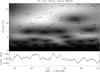 |
Fig. 4. Wavelet spectrum computed from the 2013–2014 MOST data. Edge effects are present beyond the white broken lines. |
3.3. Wavelet analysis of the MOST FU Ori data
To obtain a uniform data sampling required for the wavelet analysis of the star, we interpolated with splines the 344 mean-orbital data points into a grid of 389 equally spaced points at 0.14088 d intervals. We present the results obtained with the Morlet-6 wavelet in Fig. 4; it shows the spectrum for the relevant period range up to 17 d. The re-sampled light curve is plotted directly below the wavelet spectrum for clarity. The spectrum confirms primary characteristics of light curve segments, as defined in Sect. 3.1. The main reservation is that the 11.4 d modulation during Segment III is not present in the spectrum; instead we see a 5.5 d modulation; this discrepancy is most likely due to the finite length of the run. Similarly, we also observe a false ∼5 d periodicity during Segment I, which is roughly half of the major 10.5–11 d double-peaked quasi-periodicity.
To better illustrate the period shortening in Segment II and in the 2010 light curve (Table A.21), in Fig. 5 we additionally show fragments of both available MOST light curves with intervals P between consecutive minima and maxima of the sine-like waves. The new analysis reveals that the short-periodic oscillation seen in the 2010–2011 light curve is more complex than that which appeared in our first paper (Siwak et al. 2013). We now see a 1.08 d single wave that appeared in the middle of the wave train. It could be either due to two independent, overlapping wave trains of similar periods (the maximum at HJD-2 455 500 ≈ 48.5 may be double-peaked) or a single event in the disc or on the star. According to our previous interpretation (Siwak et al. 2013), the entire wave train showed period shortening from 2.4 to 2.2 d and this estimate was only based on the blurred wavelet spectrum. Currently, the light curve shows the period shortening from about 2.8 to 2.0–2.1 d, with some perturbations at about HJD-2 455 500 ≈ 53–56, as noticed above. It is also possible that the period shortening took place from 2.8 to 1.08 d, and later started to increase to 2.1 d.
We shortly conclude that these short-periodic sine-like oscillations were so far clearly observed in precise space-based light curves only for a limited time and they always showed clear instances of period changes, usually shortening. This suggests that they were not produced owing to the appearance of many independent flickering events in the disc, but were driven by a mechanism leading to coherent light variations.
3.4. Colour-magnitude relations from the ground-based data
To investigate the colour-magnitude relations for FU Ori, it is more convenient to utilise the Johnson V-filter standardised magnitudes, as obtained at SAAO and MSO. The effective wavelength of the V filter is similar to that of the MOST broadband filter and lies roughly in the middle of the investigated wavelength range. Although internally more accurate, the MOST magnitudes are linked to the BVRI data through the de-trending operation, as described in Sect. 2.1. The colour indices that we consider are U − V, B − V, V − Rc, V − R, V − Ic and V − I. Similar diagrams were also prepared for the MSO observations obtained in the Strömgren uvy filters, which were left in the instrumental system. Because of the similarity of the effective wavelengths, the Δy − Δ(u − y) and Δy − Δ(v − y) diagrams are closely related with the V − (U − V) and V − (B − V) colour-magnitude diagrams.
We do not show colour-magnitude diagrams prepared with the use of all data points as they contain a mix of effects from various light variability patterns that were observed at both observatories through different time spans. As announced in Sect. 1, to investigate colour-period relation we need to focus on colour-magnitude diagrams prepared for the pre-defined light curve segments; only such an approach allows us to make a link between variability patterns well defined in the MOST light curve and variability of their colour indices as a function of V and y-filter brightness. We show colour-magnitude diagrams constructed from SAAO (Figs. 6a,d,e,f) and (separately) from MSO data (Figs. 6b,c,g,h,i) to highlight distinct properties of the three individual segments; these distinct properties are best visible in V − (U − V), V − (B − V) and in corresponding Δy − Δ(u − y) and Δy − Δ(v − y) diagrams, which show that especially the points obtained during Segment I occupy separate regions. Whenever an unambiguous fit of a linear function (weighted by the V or y filter and colour index errors) was possible, we give numerical values of the slope coefficients s and Pearson’s correlation coefficients rp both for combined and separate MSO and SAAO data sets (Fig. 7). Although a limited number of data points cause the significance of each separate fit to be low, we stress that we obtained the same tendencies for each of the three independent photometric systems; only the slope for the V − (V − I) relation constructed from MSO data is negative (Fig. 7f), but this is mostly due to its non-uniform coverage with data points. We also note that the slopes obtained from our data are in qualitative accordance with the slopes obtained from the by far much more numerous multi-season data set by Kenyon et al. (2000). These authors found −0.40(14) for the V − (U − B), −0.12(2) for the V − (B − V), and 0.15(2) for the V − (V − R) relations.
Figures 7a–d prepared for Segment I of the light curve show evidence for negative slopes in the V − (U − V), Δy − Δ(u − y), Δy − Δ(v − y) and V − (B − V) diagrams. This tendency is seen both for the SAAO and for the MSO data. The V − (V − Rc) and V − (V − Ic) diagrams (Figs. 7e,f) show tendencies for zero and positive slopes, respectively. We note that the ground-based observations obtained at the MSO in two photometric systems cover the full range of Segment I variability, while at SAAO ground-based observations were only collected during the second half.
The colour-magnitude diagrams for Segment II do not show any dependency (and therefore they are not shown here). Although we made an attempt to remove the downward trend in V-filter data visible through this time interval by a parabolic fit, the large errors of the few ground-based measurements, in comparison with the mean amplitude of the sine-like variation of only 0.0055 mag (in the MOST system), exclude the possibility of finding any significant trends. We can only state that amplitudes in BVRcIcRI filters were roughly constant. We arrived at this conclusion just by looking in Figs. 8b–e, where we plot the arbitrarily shifted MOST and ground-based light curves. We note that the U-filter data show the signature of about a twice larger amplitude than observed by MOST and in the remaining Johnson filters (Figs. 8a,f).
The colour-magnitude diagrams for Segment III (Figs. 7g–i) show similar relations as those for Segment I. We consider the results obtained by the least-square fits to the combined data sets only because of the very limited number of measurements in each separate sample. The scatter in the V − (U − V) diagram (Fig. 6a) is very large and we were unable to determine any relation. The data points in the related Δy − Δ(u − y) and Δy − Δ(v − y) diagrams are slightly less scattered (Figs. 6b,c). They do not seem to contradict the statement that slopes in Segment III show similar wavelength dependency as in the Segment I diagrams.
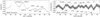 |
Fig. 5. Short-periodic fragments of 2013 and 2010 MOST light curves. In both cases maxima and minima were localised by eye to about 0.02 d, which leads to the 0.04 d uncertainty of each indicated temporal period P value. Modulations seen at the beginning are marked by “?” as they occurred prior the official start of Segment II. |
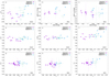 |
Fig. 6. Colour-magnitude diagrams for FU Ori prepared from data obtained during Segments I, II, and III, as defined in Sect. 3.1. |
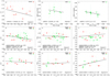 |
Fig. 7. Colour-magnitude diagrams for FU Ori specifically prepared for the first and the third Segment, as defined in Sect. 3.1. A linear least-squares weighted fit is shown and the numerical values of slopes with asymptotic standard error(s) in parentheses are given. Pearson correlation coefficients are also shown. |
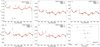 |
Fig. 8. Comparison of Segment II of the MOST light curve with UBVRcIcRI data obtained at ground-based observatories. Last panel: V − (U − V) diagram for this segment; the diagram indicates on larger variability amplitude in U- than in V filter. |
3.5. Search for origins of light variations using a disc and star light synthesis model
Apart from the phenomenological considerations presented above, we decided to construct a simple disc and star light synthesis model to pinpoint the source of light variations in FU Ori analytically. Our model (see in Appendixes A and B for full description), is similar to that constructed by Zhu et al. (2007). The major difference is that we use PHOENIX library of spectral intensities for ordinary supergiants (Husser et al. 2013). By means of our model we calculated synthetic amplitudes in Johnson filters for all light curve Segments, assuming that either hotspots on the star or disc inhomogeneities are responsible for observed light variations.
3.5.1. Testing the accretion hotspot scenario
According to the idea of Kenyon et al. (2000) and Audard et al. (2014), flux modulations induced by the changing visibility of hotspots on the star could potentially be noticed despite the prevailing disc light and lead to quasi-periodic variability, with amplitudes suppressed from 1 to 2 mag (as for CTTS), to a few hundredths of a magnitude (as for FU Ori). Though such a mechanism was excluded for past FU Ori data by Kenyon et al. (2000), it may occasionally operate in this star even though the magnetosphere in FU Ori is heavily compressed and much smaller than in typical CTTS (Königl et al. 2011). To check the hotspot scenario, we calculated synthetic amplitudes caused by rotation of a spotted star for each of the Johnson–Cousins filters to compare the results with our observations. We considered possible values of the stellar radius (R⋆) in the range 1.5–2.0 R⊙ along with several values (3500–4000 K) of effective temperatures of the stellar photosphere ( ), but finally we decided to fix the parameters at
  = 4000 K and R⋆ = 2 R⊙.
The hotspot was assumed to lie at 50 deg latitude to let the whole spot hide behind the star and lead to the variability shape observed in Segment I. The hotspot banana-shape was approximated in our model by a spherical rectangle with width of ∼8 deg in latitude and ∼60 deg in longitude, as suggested by the three-dimensional magnetohydrodynamical numerical simulations of Kulkarni & Romanova (2013). We stress that detailed values of these parameters, and whether the shape and position is typical for stable or unstable accretion regimes considered by the authors, do not impact our results in a significant way. We performed computations with typical hotspot temperatures in the range 7000–12 000 K using corresponding PHOENIX intensities, although a more detailed treatment should also include emission lines calculated by Dodin (2018). For each hotspot temperature, a corresponding set of linear limb darkening coefficients for Johnson filters was applied (Diaz-Cordoves et al. 1995; Claret et al. 1995).
Synthetic amplitudes of light variations for three selected hotspot temperature values Tspot are presented in Table 3. A strong wavelength-amplitude dependency is obvious for all considered cases. The amplitudes are highest for the U filter and decrease rapidly as the wavelength increases. This is in conflict with our observations (Figs. 1b, 2 and 6), which show similar amplitudes for almost all segments. Moreover, more detailed analysis revealed smaller amplitudes observed in ultraviolet and blue bands during Segments I and III (Figs. 7a–d,g). For this reason, we can firmly state that rotation of the stellar surface with hotspots on the photosphere is not responsible for the longer family of light variations observed in 2013–2014. This finding is also true for the eight day event observed in the first MOST light curve of FU Ori, where its MOST filter amplitude was found to be larger than that measured in the MSO Strömgren vb filters (Siwak et al. 2013).
The result obtained above may also suggest three other possibilities. First, hotspots are fairly uniformly distributed on the stellar surface, second they are not always formed on the star, and third their effective temperatures are only slightly larger than the effective temperature of the stellar photosphere. We think that the second possibility may be true for FU Ori. During Segment II the U-filter amplitude appears to be twice as large as in the remaining filters. Although the amplitudes in BVRcIc filters seem to be very similar, we state that these data are not accurate enough to exclude the hotspot scenario for this segment with full certainty; the significant elongation in y-axis seen in the V − (U − V) colour-magnitude diagram (Fig. 8f) may suggest the presence of hot radiation sources. We note that similar behaviour was also found in TW Hya. During March 9, 2016 some short-term hotspots appeared on the star as a consequence of inhomogeneous accretion. Whilst the V − (B − V) relation remained stable over the entire night, the corresponding V − (U − V) colour-magnitude diagram showed two separate relationships (see in Fig. 10 in Siwak et al. 2018).
Synthetic amplitudes in magnitudes predicted for the rotating spotted stellar surface for Johnson–Cousins filters for three selected hotspot temperatures Tspot.
3.5.2. Testing the disc inhomogeneity scenario
In the first paper of this series we proposed that given the visibility inclination of 55 deg, some surface and/or disc temperature inhomogeneities, which appear from the interactions of stellar magnetosphere with the disc plasma and then disappear within the disc dynamical timescale, may cause quasi-periodic flux modulations, as they revolve around the star. We also claimed that variation of their colour indices versus MOST (or e.g. V-filter) magnitude may depend on sizes and locations of the inhomogeneities in the disc and lead to the colour-period relation.
We propose to approximate these inhomogeneities by structures similar to spiral arms or rings, recently imaged in protoplanetary discs of young stars by ALMA (Pérez et al. 2016), VLT-SPHERE (Benisty et al. 2015; Stolker et al. 2016; Avenhaus et al. 2018), and Gemini-GPI and Magellan-MagAO (Follette et al. 2017). We believe that two different inhomogeneities on opposite sides of the inner disc, or a single inhomogeneity seen either behind or in front of the star, may lead to the double-peaked light features of various amplitudes, as observed in Segment I of the 2013–2014 MOST light curve. If this is the case, in the flat surface disc model presented in this work, the longitudinal flux distribution of disc annuli disturbed by such inhomogeneities could be parameterised by local declines and increases of its temperature with respect to the value Teff(R), predicted for a steadily accreting disc, and given by Eq. (A.2)1. Illumination of such disc inhomogeneities by the flux emerging from the innermost disc and even the central star may additionally increase their brightness contrast. Let us consider the revolution of one inhomogeneity around the star, as our multi-colour data are sensitive only to variability caused by the higher amplitude light modulation in Segment I; such a structure can be approximated assuming that the second half of the disturbed disc ring is brighter than the first half. This situation can be parameterised with the use of dimensionless factor ΔT = |T(R)−Teff(R)|/Teff(R) as follows: (2)
(2)
where  and
and  define the inner and outer radius of a disc ring, in which the real effective temperatures T(R) deviate by ΔT from these predicted by Eq. (A.2), while π is an a priori chosen azimuthal angle φ, where the temperature deviation sign changes. Rotation of the disc inhomogeneity around the star is controlled by variable phase, i.e. φ → φ + Δφ. By estimating the size of the inhomogeneous disc area (contained between
  and
and  ) for a set of small or moderate ΔT, it would be possible to obtain the observed amplitude in V filter and colour index variations with respect to the V-filter synthetic magnitudes, i.e. consistent with all colour-magnitude diagrams.
We searched the parameter space manually with step of 0.05 in ΔT for Segments I and III, and 0.01 for Segment II. The same ΔT was always assumed for all filters. A step of ΔR = 1 R⊙ was used to estimate  as well as an optimal width of the disc inhomogeneity
  . We obtained the following results for the three pre-defined light curve segments:
-
1.
To reproduce the largest 0.07 mag variations and colour-magnitude diagrams for Segment I, we found that effective temperatures in disc annuli between 16 and 20 R⊙ must deviate by ΔT ≈ 0.2. This distance is similar to the preliminary mid-inhomogeneity radius of 20 R⊙, which was obtained using blackbody approximation instead of model atmospheres, as briefly stated in Siwak et al. (2017). Degeneracy between ΔT and the position and size of the perturbed area did not turn out to be significant. An increase of the disc inhomogeneity size simultaneously with decrease of ΔT (and vice versa) results in colour-magnitude diagrams that do not match those observed. Similarly, attempts to set the inhomogeneous disc area either very close to the star (6–8 R⊙) or at a greater distance (25–30 R⊙) were also completely unsuccessful: they resulted in all positive or all negative values of slopes in synthetic colour-magnitude diagrams, respectively. We present synthetic colour-magnitude diagrams and their comparison with the best-defined SAAO observations in Fig. 9. We stress that they also match well most of the MSO and the combined SAAO and MSO colour-magnitude diagrams. We note that for this solution, synthetic amplitudes of V-filter light variations are also almost identical to those observed. The numerical values of slopes of synthetic colour-magnitude diagrams shown in Fig. 9 are as follows: −0.40 for V − (U − V), −0.16 for V − (B − V), +0.03 for V − (V − Rc), and +0.23 for V − (V − Ic). The theoretical values of the colour indices are also similar to those observed. The discrepancies, i.e. constant shifts in colour indicies (e.g. −0.10 mag for the V − (U − V) diagram), applied manually to match observations, are indicated in all four panels in Fig. 9. These discrepancies result from imperfections of the model such as the choice of spectral intensities for ordinary supergiants, zero-point calibration and interstellar extinction estimate errors, and limited availability of the stellar models below 2300 K.
-
2.
The similarity of amplitudes of MOST and ground-based UBVRcIc light curves in Segment II may also suggest their disc origin. Unfortunately, the lack of any trends in the colour-magnitude diagrams severely limits precision of localisation of the inhomogeneous plasma parcels by means of the light synthesis model. Therefore, we can rely on the coarse constancy of their amplitudes, as inferred from Fig. 8b to e. Even though most similar amplitudes in BVRcIc filters are obtained from our model for disc inhomogeneities located between 13 and 20 R⊙, the higher observed amplitude in U filter (Figs. 8a,f) may suggest a slightly closer location of between 12 and 15 R⊙. The observed amplitudes were roughly reproduced by our model for ΔT = 0.03 (Fig. 10). Although the lack of precise U-filter data seriously limits precision of this estimate, the location of the inhomogeneity at the inner disc rim, as expected from the short 3–1.38 d period of this wave train, can be excluded within the disc model of Zhu et al. (2007). Otherwise we would observe almost constant light in the Ic filter, and the amplitude would gradually increase with decreasing effective wavelengths of the remaining filters, as suggested by the first panel in Fig. 10.
-
3.
The same conclusion as for Segment I can also be true for Segment III. This is due to similarity of trends observed in respective colour-magnitude diagrams for Johnson–Cousins filters, as shown by the s values (Figs. 7g,h,i). The large scatter of U-filter data makes it impossible to find any firm relation from the V − (U − V) diagram (Fig. 6a), but the slope appears to be negative on the auxiliary Δy − Δ(v − y) diagram (Fig. 6c). Therefore we conclude that Segment III light variations could arise somewhere at the distance of 14–19 R⊙ from the star (for ΔT ≈ 0.15).
We did not consider disc inclinations other than 55 deg and temperature distributions corresponding to a range of MṀ values. For instance, the variability shape observed in Segments I and III could be fairly well reconstructed for disc inclinations closer to 70 deg, as derived for FU Ori by Gramajo et al. (2014); such extended computations may be meaningful when more precise multi-colour observations are available from future space telescopes.
The main conclusion of this model is not to pay too much attention to the exact numbers obtained, but rather to point out that long-periodic (10–11 d) families do not arise either very close (∼5 − 10 R⊙) or very far from the star (∼30 − 40 R⊙), but near 15–20 R⊙. More accurate modelling, including reliable three-dimensional approximation of disc inhomogeneity instead of its crude parameterisation by ΔT factor, will allow us to refine these results in the future. In this paper we assume that ΔT parameter automatically takes into account all phenomena related to the fact that real disc inhomogeneities probably have the form of waves or warps. Once illuminated by the inner disc, they may cast shadows on more distant parts of the disc.
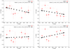 |
Fig. 9. Comparison of observed (circles, the SAAO data only) and synthetic (squares) colour-magnitude diagrams for Segment I. |
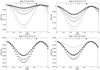 |
Fig. 10. Sample of synthetic light curves in UBVRcIc filters used during the localisation process of Segment II light variations. Most similar amplitudes in BVRcIc filters are obtained for disc inhomogeneities located between 13 and 20 R⊙, but the slightly higher amplitude in the U filter may suggest somewhat closer localisation, from 12 to 15 R⊙. The values used in a given model (ΔT, |


 |
Fig. 11. Picture proposed for a qualitative explanation of the Segment I variability. The lighter semi-ring represents the 16–20 R⊙ disc inhomogeneity in three rotational phases. The disc fluxes calculated for V filter are expressed in greyscales (as defined on respective bars) and are left in temporary model units; they are also slightly affected by limitations of our plotting software. The stellar flux is expressed arbitrarily; the stellar radius was set to 1.5 R⊙. |
4. Discussion
The new 2013–2014 MOST light curve of FU Ori was collected over a twice as long interval as the first, gathered in the 2010–2011 season. This enabled us to identify three families of light variations characterised by different quasi-periods and variability patterns: namely Segments I, II, and III, as defined in Sect. 3.1. The colour-magnitude diagrams for respective segments constructed from the uvyUBVRcIcRI data taken simultaneously from the ground were used to pinpoint mechanisms leading to the observed variability.
4.1. Results for long-periodic light variations
The light variations observed in Segment I and Segment III are probably driven by the same mechanism, as inferred from analysis of their colour-magnitude diagrams (Figs. 7 and 9). Using the disc and star light synthesis model, we ruled out the possibility that the QPOs seen in Segment I could be due to changing visibility of accretion hotspots on the star (Sect. 3.5.1). Instead, we argue that they could arise owing to revolution of the disc inhomogeneity located between 16 and 20 R⊙ (see in Sect. 3.5.2 and in Fig. 11). Our observations indicate that its lifetime does not exceed several revolutions around the star. We note that the average radius 18 R⊙ of the 4 R⊙ wide inhomogeneity obtained from the light synthesis model for the 10.75 d quasi-period is by 4.3 R⊙ larger than the Keplerian radius of 13.7 R⊙, expected for the stellar mass of 0.3 M⊙. This small disagreement disappears if we assume 0.7 M⊙ for the central star, in accordance with Gramajo et al. (2014). Assuming that Segment III was also due to Keplerian revolution, the stellar mass derived for average radius (16.5 R⊙) of the inhomogeneity (14–19 R⊙) would be smaller, i.e. about 0.45 M⊙. Nevertheless, no one can consider this particular result as significant owing to the doubts concerning the quasi-periodic nature of these light variations, as described in point 3 of Sect. 3.1.
The formation mechanism of disc inhomogeneities at the distance of 0.05–0.1 AU responsible for the ∼10 − 11 d oscillations is not clear to us. These inhomogeneities could perhaps be related to a mechanism leading to FUor outbursts themselves. Recently, Liu et al. (2016) presented Subaru Hi-CIAO differential linear-polarisation imaging observations, showing large-scale asymmetrical structures around FU Ori, Z CMa, V1735 Cyg, and V1057 Cyg. Their result supports the gravitational instability of the disc as a mechanism creating spirals and clumps falling towards the star and leading to accumulation of mass near the inner disc and to enhanced accretion (see also in Vorobyov & Basu 2005, 2006; Vorobyov et al. 2015). Once the matter is slowly accumulated owing to gravitational instabilities, it may trigger thermal instabilities in the inner disc. This also activates magneto-rotational instabilities leading to the FUor-type outburst (Zhu et al. 2009). These authors calculated light curves showing small-amplitude quasi-periodic light variations after the outburst, which might be caused by convective eddies formed in the high state-low state transition region. The convection is especially strong and even penetrates the mid-plane of the disc in the regions of 0.15–0.35 AU, but is still present although confined only to the disc surface for smaller disc radii.
It is not excluded that convection eddies may be responsible for the longer family of light variations observed by MOST and earlier from the ground, as mentioned in Sect. 1. Assuming this scenario is correct, our MSO observations, lasting 194 d, also had the potential to detect quasi-periods up to 65 d long and probe light variations occurring at 50–60 R⊙ (0.25 AU). Although periodograms presented in the first panel of Fig. 3 show two wide peaks at 13–17 and 42–48 d, their significance is very low. If these longest variations really arise owing to convection eddies that are persistent for a few revolutions around the star, then their amplitudes seen in infrared filters should be larger than in visual bands.
The FUor phenomenon could also be initiated by tidal disruption of a few Jupiter mass planet, as obtained by Lodato & Clarke (2004) and Nayakshin & Lodato (2012). These authors showed that before the disc gap is opened a planet can easily migrate to the distance of ∼0.1 AU from the star; this is similar to the inhomogeneity average radius estimated for Segments I and III. The material from the planet may feed the disc through Roche lobe overflow, leading to an enhanced mass accretion and a major disc brightness increase. It is not excluded that tidal disruption of a planet may create disc inhomogeneities in close vicinity of the star. However, in these circumstances permanent rather than quasi-periodic light variations should be observed. We note that also Powell et al. (2012) considered this scenario to explain the persistent 3.6 d periodic modulation found in cross-correlation function profiles of FU Ori; this periodicity is not visible as a constant feature in the MOST light curves.
The very interesting possibility is also offered by Romanova et al. (2013), who found waves induced in the disc plasma structure from interactions with a rotating tilted magnetosphere of a star. The authors obtained two major types of solutions:
-
1.
The first is for typical CTTS, where a magnetospheric radius is similar to the co-rotation radius (see Sect. 3.2 of their paper). In this case a strong warp is formed that rotates with the stellar frequency. This scenario can be applied to AA Tau-like stars, periodically obscured by a warped disc (Bouvier et al. 1999, 2007; McGinnis et al. 2015),
-
2.
The second solution is for the case in which the magnetospheric radius is much smaller than the co-rotation radius (see Sect. 3.3 of Romanova et al. 2013). Such a situation occurs in CTTS with enhanced mass accretion, when the disc plasma pressure compresses the magnetosphere. Our guess is that the latter solution could also apply to FU Ori, as suggested by Audard et al. (2014). Although Romanova et al. (2013) claimed in Sect. 4.1 of their paper that waves created in CTTS discs cannot be directly observed because of the large brightness contrast with the dominant star, it does not apply to FU Ori, where the disc overwhelms the stellar luminosity by a hundred times2. The authors found high-frequency inner bending waves, i.e. inhomogeneities whose rotational frequency around the star is almost equal to, or slightly lower than, the Keplerian velocity of the inner disc. The waves originate only during periods of unstable accretion and are located at the inner edge of the disc. In addition, the authors also found lower frequency waves that propagate to larger distances and are sometimes enhanced at the disc co-rotation radius. The major warp, causing AA Tau-type occultations, does not appear.
If the latter solution is applicable to FU Ori, then the 10–11 d light variations observed in Segments I and III could represent modulation in the visibility of the inhomogeneity caused by a locally enhanced lower frequency wave at (or near) the disc co-rotation radius and perhaps also the stellar rotational period. We note that stable over three seasons 14.8 d periodic modulation of P Cygni profiles by the disc wind found in FU Ori spectra by Herbig et al. (2003), and later confirmed (at 13.48 d) by Powell et al. (2012), was proposed by the first authors to be the rotational period of the star. So far, our preliminary attempts to explain Segment I and III variability by axially non-symmetrical dusty disc wind parameterised by means of single (1 − ΔT) term in Eq. (2) resulted in a non-physical solution; we obtained that the light emerging from the disc semi-ring between 11 and 16 R⊙ must be almost completely absorbed. This solution maintains both the colour-period relation for the stellar mass of 0.3 M⊙, observed amplitudes, and the same values of negative and positive slopes in consecutive colour-magnitude diagrams. However, such a mechanism would lead to significant modulations of the disc rotational profiles, which would certainly have been noticed by previous authors. Coordinated space-based photometric and ground-based high-resolution spectroscopic observations may enable the study of possible relationships in the future.
4.2. Results for short-periodic light variations
Segment II of the light curve is composed of a short-period, sine-like wave train of much smaller (∼0.01 mag) amplitude. A period shortening of each successive oscillation is seen directly in the light curve. This wave train became visible at the end of Segment I as the ∼3.5 d signal, and ceased after 8–9 d, when its period shortened down to 1.38 ± 0.04 d. If this light variability is driven by the Keplerian motion of disc inhomogeneities drifting to the inner disc parts, as previously deduced from its continuously decreasing period (Siwak et al. 2013), then for the stellar mass of 0.3 M⊙ we obtain the value of the inner disc radius of 3.5 R⊙ or 4.6 R⊙ for 0.7 M⊙. These values are also in accord with interferometric observations of Malbet et al. (2005), who obtained  R⊙, and with the value of the stellar radius of 3.6 R⊙ derived by Königl et al. (2011).
The short-periodic sine-like variability pattern revealed by MOST in the 2010–2011 light curve, was re-analysed in Sect. 3.3. The conclusions are somewhat different from the preliminary findings by Siwak et al. (2013). The lower values of periods obtained in Sect. 3.3 may be used for refinement of the inner disc radius value obtained in Siwak et al. (2013): if 2.1 d is the lower period limit then the change in inner disc radius value is small, from 4.8 to 4.5 R⊙ for 0.3 M⊙, or 6 R⊙ for 0.7 M⊙. Assuming that the 1.08 d value was due to the revolution of a plasma parcel with a local Keplerian speed at the inner disc radius, the respective radii would be equal to 3 R⊙ or 3.9 R⊙.
Unexpectedly, the above interpretation regarding the origin of (at least) the 2013–2014 short-periodic light variations was questioned by the disc and star light synthesis model. We found that similarity of the amplitudes observed in UBVRcIc filters (Figs. 8a–e) can only be explained by the changing visibility of the disc inhomogeneities parameterised by ΔT = 0.03 − 0.04 and located between 12 and 15 R⊙. This is in strong conflict with the location predicted with the assumption of purely Keplerian motion of the plasma parcels in the innermost disc region (∼3 − 8 R⊙), as discussed above. To avoid this conflict, we attempted to explain these light variations by assuming that they are caused by modulations of the innermost disc flux. For example, we made an attempt to explain these variations by a dusty disc wind, approximated by means of a single term in Eq. (2), i.e. (1 − ΔT) × Teff(R), and moderate-to-large values of ΔT; however this was also unsuccessful.
We conclude that these short-periodic light variations cannot be assigned to high-frequency waves (see in in point 2 of Sect. 4.1) assuming that the temperature distribution in the disc follows the model of Zhu et al. (2007). If these QPOs really arise between 12 and 15 R⊙, then they cannot be driven by Keplerian revolution of the disc inhomogeneities. In these circumstances our model obviously should not be used to describe short-periodic oscillations. Maybe a clue to the real mechanism is hidden in the fact that light variations observed in Segment I smoothly transfer into the Segment II sine-like wave with decreasing amplitude and period. This may suggest that these two light curve segments were in fact physically linked. It is not excluded that the first (Segment I) was due to the Keplerian revolution of a disc inhomogeneity around the star, while the second (Segment II) was the signature of some hypothetical disc plasma oscillations, excited during dissipation of the previously dominating major disc inhomogeneity.
We suppose, however, that a physically more consistent explanation can be offered by the assumption that the magnetospheric gap in FUors is not always devoid of visible light sources. The inclusion of this possibility would require proper modification of our light synthesis model in the future.
As mentioned in Sect. 1, to explain the observed colour-magnitude relations in UBVR filters, Kenyon et al. (2000) proposed that the light variations in FU Ori mostly arise in the narrow zone between the radius, where the disc temperature reaches its maximum, and the stellar photosphere (i.e. at 1.1–1.2 R⋆ in their model units). This was in accordance with their Monte Carlo computations indicating that random fluctuations of a characteristic timescale no longer than 1 d dominate in the light curve. However, our MOST observations do not necessarily confirm this view. Quasi-periods of 1–3 d are seen only during very limited time intervals and these variations appear to be time coherent. Moreover, the existence of a typical boundary layer zone in FU Ori was later questioned by Zhu et al. (2007). Instead, it turned out that in spite of enhanced mass transfer, FU Ori may possess a small magnetosphere. Assuming that the observationally determined inner disc radius of 5 R⊙ (Malbet et al. 2005; Zhu et al. 2007) is equal to the magnetospheric radius rm, the lower limit of rm/R⋆ ≈ 1.4 was derived by Königl et al. (2011). According to the authors this size is in accordance with the result of Donati et al. (2005), who measured the poloidal component of the inner disc magnetic field at 1 kG. In these circumstances short-lived unstable accretion tongues rotating with the inner disc rotational frequency can be formed (Kulkarni & Romanova 2008, 2009; Blinova et al. 2016) and are expected to transfer disc plasma towards the star. If plasma carried in these tongues would be cooler by 1500–2000 K than the maximum disc temperature (6420 K), then changing visibility of these tongues could lead to the short-periodic, small-amplitude light variations of similar amplitudes in Johnson filters, as observed in Segment II (Fig. 8).
FU Ori is not the only FUor, where short-periodic QPOs were observed. The shortest detected 1.28 d period in FU Ori-type star V2493 Cyg was also attributed to Keplerian rotation of plasma parcels emerging at the disc magnetospheric radius by Green et al. (2013). Similarly, about 1 d flux modulation due to the changing visibility of two antipodal accretion hotspots on the star was found in X-ray observations of the EXor/FUor star V1647 Ori (Hamaguchi et al. 2012). The hot X-ray component in FU Ori is also variable (at 0.8 d) and viewed through heavy absorption from a disc wind or accretion stream (Skinner et al. 2010). These results appear to be in agreement with the result of Blinova et al. (2016), who found that for small magnetospheres as in FU Ori, an ordered unstable regime may create one or two tongues and related hotspots that are not fixed on the star, but rotate with the inner disc rotational frequency. This scenario would also explain period shortening observed by MOST in Segment II, by assuming that the accretion rate inside a tongue increases, as predicted by Kulkarni & Romanova (2009).
It is a matter of debate, whether about twice greater amplitude observed in U filter during Segment II definitely speaks for the so-called hotspot mechanism, at least occasionally operating in FU Ori. Accurate flux-calibrated spectra obtained simultaneously with space-based photometric (and ideally also X-ray) observations may be helpful to catch signatures of these additional hot radiation sources at short wavelengths during future occurrences of ∼1 − 3 d light variations.
5. Summary
We observed FU Ori simultaneously from space and the ground in winter 2013–2014 with the aim to determine the mechanisms leading to light variations discovered by MOST during the first run in 2010–2011. Comparison of ground-based and synthetic colour-magnitude diagrams specifically prepared for each of three distinct oscillatory patterns identified in the new light curve indicates that the longer, ∼10–11 d QPOs are most likely due to the changing visibility of disc inhomogeneities localised at a distance of about 16–20 R⊙. These inhomogeneities could represent convection eddies in the disc (Zhu et al. 2009) and/or low-frequency waves caused by interactions of a tilted stellar magnetosphere with the disc plasma and enhanced at the disc co-rotation radius (Romanova et al. 2013).
The local Keplerian periodicity in the middle (18 R⊙) of the major inhomogeneity is 11 d if we assume a stellar mass of 0.7 M⊙. This result is in reasonable agreement with the colour-period relationship claimed in Sect. 1. However, no similar agreement was obtained for the short-periodic 3–1.38 d variability. According to our light synthesis model, this variability appears to arise somewhere between 12 and 15 R⊙. The mechanism engaging Keplerian revolution of a disc inhomogeneity on a spiral orbit, however suggests a gradual approach of the inhomogeneous plasma parcel towards the star from 5.9 to 3.5 R⊙ or from 7.8 to 4.6 R⊙ assuming reasonable stellar masses of 0.3 or 0.7 M⊙, respectively. This disagreement might be temporarily resolved by assuming that one or two unstable tongues, in which disc plasma of the temperature of about 4500–5000 K is transmitted towards the star, appear in the small magnetospheric gap at least for a short time. Our U-filter observations also indicate the possibility that these short-periodic light variations may also be driven by related hotspot(s), revolving on stellar surface with the local Keplerian velocity of related tongue(s).
Further accurate broadband simultaneous photometric and spectroscopic observations are needed to clarify the issues left with a question mark in this paper. With the end of the MOST satellite activity, the next possibility to observe FU Ori should appear during the TESS mission. However, TESS will still provide single-band observations only. Unfortunately, the apertures of the BRITE satellites fleet (Weiss et al. 2014), which provides six-month-long, blue- and red-band light curves, are too small to provide data on FU Ori. Two-colour, high-precision, space-based data may be provided by UVSat (Pigulski et al. 2017). This would eliminate the problems arising from the limited accuracy of ground-based observations in the ultraviolet band, and would be very suitable for exploration of disc dynamics of the brightest FUors.
One can question the approach adopted in this model because the approximation of the disc inhomogeneities by ΔT entails the use of Iλ, whose values are not necessarily appropriate for the disturbed plasma.
We also note that Flaherty et al. (2016) found a few dozen examples of such interactions in infrared Spitzer long-term observations of young stellar objects in Chamaleon I star forming region.
Acknowledgments
This study was based on (1) data from the MOST satellite, a Canadian Space Agency mission jointly operated by Dynacon Inc., the University of Toronto Institut of Aerospace Studies, and the University of British Columbia, with the assistance of the University of Vienna; (2) observations made at the Mount Suhora Astronomical Observatory, Cracow Pedagogical University; and (3) observations made at the South African Astronomical Observatory. This paper also made use of NASA’s Astrophysics Data System (ADS) Bibliographic Services. MS, MW, MD, and WO are grateful to the Polish National Science Centre for the grant 2012/05/E/ST9/03915. GS is grateful for the Polish National Science Centre for the grant 2011/03/D/ST9/01808. Polish participation in SALT is funded by grant No. MNiSW DIR/WK/2016/07. The Natural Sciences and Engineering Research Council of Canada supports the research of DBG, JMM, AFJM, and SMR. Additional support for AFJM was provided by FQRNT (Québec). CC was supported by the Canadian Space Agency. RK and WWW are supported by the Austrian Science Funding Agency (P22691-N16). MS acknowledges Dr. Francois van Wyk and the entire SAAO staff for their hospitality, as well as the observers, who obtained observations at the MSO during single nights, i.e. Dr. hab. Andrzej Baran, mgr. Michał Żejmo, and Dr. Jan Janik. Special thanks are also due to an anonymous referee for highly useful suggestions and comments on the previous version of the paper.
References
- Audard, M., Abraham, P., Dunham, M. M., et al. 2014, Protostars and Planets VI, eds. H. Beuther, R. S. Klessen, C. P. Dullemond, & T. Henning (Tucson: University of Arizona Press), 914, 387 [NASA ADS] [Google Scholar]
- Avenhaus, H., Quanz, S. P., Garufi, A., et al. 2018, ApJ, 863, 44 [NASA ADS] [CrossRef] [Google Scholar]
- Benisty, M., Juhasz, A., Boccaletti, A., et al. 2015, A&A, 578, L6 [NASA ADS] [CrossRef] [EDP Sciences] [Google Scholar]
- Bessel, M. S. 1990, PASP, 102, 1181 [NASA ADS] [CrossRef] [Google Scholar]
- Blinova, A. A., Romanova, M. M., & Lovelace R. V. E. 2016, MNRAS, 459, 2354 [NASA ADS] [CrossRef] [Google Scholar]
- Bouvier, J., Chelli, A., Allain, S., et al. 1999, A&A, 349, 619 [NASA ADS] [Google Scholar]
- Bouvier, J., Alencar, S. H. P., Boutelier, T., Dougados, C., & Balog, Z. 2007, A&A, 463, 1017 [NASA ADS] [CrossRef] [EDP Sciences] [Google Scholar]
- Cardelli, J. A., Clayton, G. C., & Mathis, J. S. 1989, AJ, 345, 245 [Google Scholar]
- Claret, A., Diaz-Cordoves, J., & Gimenez, A. 1995, A&AS, 114, 247 [NASA ADS] [Google Scholar]
- Clarke, C., Lodato, G., Melnikov, S. Y., & Ibrahimov, M. A. 2005, MNRAS, 361, 942 [Google Scholar]
- Crause, L. A., Carter, D., Daniels, A., et al. 2016, Proc. SPIE, 9908, 990827 [CrossRef] [Google Scholar]
- Diaz-Cordoves, J., Claret, A., & Gimenez A. 1995, A&AS, 110, 329 [NASA ADS] [Google Scholar]
- Dodin, A. 2018, MNRAS, 475, 4367 [NASA ADS] [CrossRef] [Google Scholar]
- Donati, J.-F., Paletou, F., Bouvier, J., & Ferreira, J. 2005, Nature, 438, 466 [NASA ADS] [CrossRef] [PubMed] [Google Scholar]
- Flaherty, K. M., DeMarchi, L., Muzerolle, J., et al. 2016, ApJ, 883, 104 [NASA ADS] [CrossRef] [Google Scholar]
- Follette, K. B., Rameau, J., Dong, R., et al. 2017, AJ, 153, 264 [NASA ADS] [CrossRef] [Google Scholar]
- Fukugita, M., Ichikawa, T., Gunn, J. E., et al. 1996, AJ, 111, 1748 [NASA ADS] [CrossRef] [Google Scholar]
- Gramajo, L. V., Rodón, J. A., & Gómez, M. 2014, AJ, 147, 140 [NASA ADS] [CrossRef] [Google Scholar]
- Green, J. D., Robertson, P., Baek, G., et al. 2013, AJ, 764, 22 [NASA ADS] [CrossRef] [Google Scholar]
- Hamaguchi, K., Grosso, N., Kastner, J. H., et al. 2012, ApJ, 754, 32 [NASA ADS] [CrossRef] [Google Scholar]
- Hartmann, L. 1998, Accretion Processes in Star Formation (Cambridge, UK: Cambridge University Press) [Google Scholar]
- Hartmann, L., & Kenyon, S. J. 1985, ApJ, 299, 462 [NASA ADS] [CrossRef] [Google Scholar]
- Hartmann, L., & Kenyon, S. J. 1996, ARA&A, 34, 207 [NASA ADS] [CrossRef] [EDP Sciences] [MathSciNet] [Google Scholar]
- Herbig, G. H. 1977, ApJ, 217, 693 [NASA ADS] [CrossRef] [Google Scholar]
- Herbig, G. H., Petrov, P. P., & Duemmler, R. 2003, ApJ, 595, 384 [NASA ADS] [CrossRef] [Google Scholar]
- Husser, T.-O., Wende-von Berg, S., Dreizler, S., et al. 2013, A&A, 553, A6 [NASA ADS] [CrossRef] [EDP Sciences] [Google Scholar]
- Ibragimov, M. A. 1993, Astrophysics, 35, 257 [NASA ADS] [CrossRef] [Google Scholar]
- Kenyon, S. J., Hartmann, L., & Hewett, R. 1988, ApJ, 325, 231 [NASA ADS] [CrossRef] [Google Scholar]
- Kenyon, S. J., Kolotilov, E. A., Ibragimov, M. A., & Mattei, J. A. 2000, ApJ, 531, 1028 [NASA ADS] [CrossRef] [Google Scholar]
- Kolotilov, E. A., & Petrov, P. P. 1985, Sov. Astron. Lett., 11, 385 [Google Scholar]
- Königl, A., Romanova, M. M., & Lovelace, R. V. E. 2011, MNRAS, 416, 757 [NASA ADS] [Google Scholar]
- Kulkarni, A. K., & Romanova, M. M. 2008, MNRAS, 386, 673 [NASA ADS] [CrossRef] [Google Scholar]
- Kulkarni, A. K., & Romanova, M. M. 2009, MNRAS, 398, 701 [NASA ADS] [CrossRef] [Google Scholar]
- Kulkarni, A. K., & Romanova, M. M. 2013, MNRAS, 433, 3048 [NASA ADS] [CrossRef] [Google Scholar]
- Liu, H. B., Takami, M., Kudo, T., et al. 2016, Sci. Adv., 2, e1500875 [Google Scholar]
- Lodato, G., & Clarke, C. J. 2004, MNRAS, 353, 841 [NASA ADS] [CrossRef] [Google Scholar]
- Luybarskii, Y. E. 1997, MNRAS, 292, 679 [NASA ADS] [CrossRef] [Google Scholar]
- Malbet, F., Lachaume, R., Berger, J.-P., et al. 2005, A&A, 437, 627 [Google Scholar]
- Matthews, J. M., Kusching, R., Guenther, D. B., et al. 2004, Nature, 430, 51 [NASA ADS] [CrossRef] [PubMed] [Google Scholar]
- McGinnis, P. T., Alencar, S. H. P., Guimaraes, M. M., et al. 2015, A&A, 577, A11 [NASA ADS] [CrossRef] [EDP Sciences] [Google Scholar]
- Menzies, J. W., Cousins, A. W. J., Banfield, R. M., & Laing, J. D. 1989, SAAO Circ., 13, 1 [NASA ADS] [Google Scholar]
- Motl, D. 2011, http://c-munipack.sourceforge.net [Google Scholar]
- Nayakshin, S., & Lodato, G. 2012, MNRAS, 426, 70 [NASA ADS] [CrossRef] [Google Scholar]
- Pérez, L. M., Carpenter, J. M., Andrews, S. M., et al. 2016, Science, 353, 1519 [NASA ADS] [CrossRef] [Google Scholar]
- Pigulski, A., Baran, A., Bzowski, M., et al. 2017, Proc. PAS, 2nd BRITE Sci. Conf., 5, 76 [Google Scholar]
- Powell, S. L., Irwin, M., Bouvier, J., & Clarke, C. J. 2012, MNRAS, 426, 3315 [NASA ADS] [CrossRef] [Google Scholar]
- Pueyo, L., Hillenbrand, L., Vasisht, G., et al. 2012, ApJ, 757, 57 [Google Scholar]
- Pringle, J. E. 1981, ARA&A, 19, 137 [NASA ADS] [CrossRef] [Google Scholar]
- Romanova, M. M., Ustyugova, G. V., Koldoba, A. V., & Lovelace, R. V. E. 2004, ApJ, 610, 920 [NASA ADS] [CrossRef] [Google Scholar]
- Romanova, M. M., Ustyugova, G. V., Koldoba, A. V., & Lovelace, R. V. E. 2013, MNRAS, 430, 699 [NASA ADS] [CrossRef] [Google Scholar]
- Rowe, J. F., Matthews, J. M., Seager, S., et al. 2006, ApJ, 646, 1241 [NASA ADS] [CrossRef] [Google Scholar]
- Rucinski, S. M., Matthews, J. M., Kuschnig, R., et al. 2008 MNRAS, 391, 1913 [NASA ADS] [CrossRef] [MathSciNet] [Google Scholar]
- Sicilia-Aguilar, A., Fang, M., Roccatagliata, V., et al. 2015, A&A, 580, A82 [NASA ADS] [CrossRef] [EDP Sciences] [Google Scholar]
- Sipos, N., Ábrahám, P., Acosta-Pulido, J., et al. 2009, A&A, 507, 881 [NASA ADS] [CrossRef] [EDP Sciences] [Google Scholar]
- Siwak, M., Rucinski, S. M., Matthews, J. M., et al. 2011, MNRAS, 410, 2725 [NASA ADS] [CrossRef] [Google Scholar]
- Siwak, M., Rucinski, S. M., Matthews, J. M., et al. 2013, MNRAS, 432, 194 [NASA ADS] [CrossRef] [Google Scholar]
- Siwak, M., Rucinski, S. M., Matthews, J. M., et al. 2014, MNRAS, 444, 327 [NASA ADS] [CrossRef] [Google Scholar]
- Siwak, M., Ogloza, W., Rucinski, S. M., et al. 2016, MNRAS, 456, 3972 [NASA ADS] [CrossRef] [Google Scholar]
- Siwak, M., Rucinski, S. M., Matthews, J. M., et al. 2017, Proc. PAS, 2nd BRITE Sci. Conf., 5, 214 [Google Scholar]
- Siwak, M., Ogloza, W., Moffat, A. F. J., et al. 2018, MNRAS, 478, 758 [NASA ADS] [CrossRef] [Google Scholar]
- Skinner, S. L., Güdel, M., Briggs, K. R., & Lamzin, S. A. 2010, ApJ, 722, 1654 [NASA ADS] [CrossRef] [Google Scholar]
- Stetson, P. B. 1987, PASP, 99, 191 [NASA ADS] [CrossRef] [Google Scholar]
- Stolker, T., Dominik, C., Avenhaus, H., et al. 2016, A&A, 595, A113 [NASA ADS] [CrossRef] [EDP Sciences] [Google Scholar]
- Vorobyov, E. I., & Basu, S. 2005, ApJ, 633, L137 [NASA ADS] [CrossRef] [Google Scholar]
- Vorobyov, E. I., & Basu, S. 2006, ApJ, 650, 956 [NASA ADS] [CrossRef] [Google Scholar]
- Vorobyov, E. I., & Basu, S. 2015, ApJ, 805, 115 [NASA ADS] [CrossRef] [Google Scholar]
- Walker, G. A. H., Matthews, J. M., Kuschnig, R., et al. 2003, PASP, 115, 1023 [NASA ADS] [CrossRef] [Google Scholar]
- Warmels, R. H. 1991, PASP Conf. Ser., 25, 115 [NASA ADS] [Google Scholar]
- Weiss, W. W., Rucinski, S. M., Moffat, A. F. J., et al. 2014, PASP, 126, 573 [NASA ADS] [CrossRef] [Google Scholar]
- Zhu, Z., Hartmann, L., Calvet, N., et al. 2007, ApJ, 669, 483 [NASA ADS] [CrossRef] [Google Scholar]
- Zhu, Z., Hartmann, L., Gammie, C., & McKinney, J. C. 2009, ApJ, 701, 620 [NASA ADS] [CrossRef] [Google Scholar]
Appendix A:
Description of the model
The disc geometry of the model is assumed as in Sect. 3 of Zhu et al. (2007), i.e. the disc vertical height H is a function of the disc radius R, measured from the central star, given by (A.1)
(A.1)
where the thickness of the inner disc, presumably truncated by the stellar magnetosphere at Rinn = 5 R⊙, is assumed to be H0 = 0.1 Rinn. The distribution of the disc effective temperature Teff as a function of disc radius R is assumed for the stationary accretion case (Pringle 1981)![Mathematical equation: $ \begin{aligned} T_\mathrm{eff}^{4}(R)= \frac{3GM{\dot{M}}}{8{\pi }{\sigma }R^{3}} \left[1-\left(\frac{R_\mathrm{inn}}{R}\right)^{\frac{1}{2}}\right], \end{aligned} $](/articles/aa/full_html/2018/10/aa33401-18/aa33401-18-eq20.gif) (A.2)
(A.2)
where G is the universal gravitation constant, M is the stellar mass, Ṁ is the mass accretion rate transferred from the disc onto the central star, and σ is the Boltzmann constant. In accordance with Zhu et al. (2007), we assume  and that the effective temperature of disc annuli located closer than 1.36 Rinn is equal to the maximum disc temperature value, calculated by Zhu et al. (2007) to be 6420 K.
The surfaces of consecutive disc annuli were approximated by surface areas of truncated cones. Subsequently, each disc annulus was divided into smaller elements, evenly distributed in azimuthal angle φ. The flux emerging from each fine element was computed taking into account its effective surface area dS = dφdR, which is a function of inclination, the orientation angle of a particular annulus with respect to the disc mid-plane, and the azimuthal angle (φ) of the centre of a surface element dS. In accord with previous works (Kenyon et al. 1988; Zhu et al. 2007), we assumed that atmospheres of consecutive disc annuli radiate in the same way as atmospheres of supergiant stars with the effective temperatures given by Eq. (3). Hence, for the flux calculations we used the emerging intensities (a full radiation field) of supergiant stars from the PHOENIX library (Husser et al. 2013). The theoretical intensities Iλ in this library are calculated for 78 values of μ = cos γ, where γ is the angle of view between the normal vector of the infinitely small element of the photosphere and the observer. The intensities are calculated with a resolution of 1 Å in wavelength and 100 K in effective temperature, starting from 500 Å and 2300 K, respectively. Special attention was given to the choice of intensities with a proper log g (in cgs units), which changed from 1.5 (6500–5300 K) through 1.0 (5200–4200 K), 0.5 (4100–3700 K), 0.0 (3600–3200 K), to −0.5 (3100–2300 K). Because of the lack of proper intensities for log g = −0.5 for the last temperature range in the library, we were forced to extrapolate the intensities for log g = 0.0 using coefficients estimated by comparison of intensities calculated for log g = −0.5 and 0.0 in the range 3200–3600 K; luckily the above operation has negligible significance for the final result. To obtain emergent intensities Iλ( μ) for each disc element dS, we interpolated the library intensities in μ and Teff to account for the full range of visibility angles γ = 46.5 − 63.6 deg and temperatures Teff = 2300 − 6420 K appropriate for our case. Finally we calculated the flux  emitted in a given direction from the disc by integration,
 (A.3)
(A.3)
where 0 ≤ φ < 2π, 5 ≤ R ≤ 44.6 R⊙. The upper limit of 44.6 R⊙ is imposed by the lack of theoretical models for temperatures lower than 2300 K in the PHOENIX library. This is fortunately not a serious limitation of our results, as the contribution of disc light emerging beyond this radius should be small. This amounted to only 2% for the I filter in the very first FU Ori disc model of Kenyon et al. (1988) and was practically equal to zero for other Johnson filters.
For the observed disc inclination of 55 deg and the inner disc radius of 5 R⊙ (Malbet et al. 2005; Zhu et al. 2007), the star can be slightly obscured by the front disc rim only for R⋆ larger than 2 R⊙. In spite that Königl et al. (2011) proposed R⋆ = 3.6 R⊙, we considered a range of smaller values between 1.5 and 2 R⊙ and effective temperatures  of 3500–4000 K, which are more typical of CTTS. The results turned out to be very weakly dependent on the parameters within the above ranges, and we finally chose the temperature of 4000 K and radius of 2 R⊙ for the central star in further calculations. To integrate the star flux (
 ), we used Iλ( μ = 1), calculated for solar metallicity [Fe/H] = 0 and log g = 4.0 from the respective PHOENIX model and then we applied the linear limb-darkening law using the coefficients from the Diaz-Cordoves et al. (1995) and the Claret et al. (1995) tables for UBVRI filters.
The emitted disc and star summed fluxes Fft in individual photometric pass bands ft ∈ {U, B, V, Rc, Ic} were determined using the transmission function profiles τλft from Bessel (1990), i.e. (A.4)
(A.4)
where λ varied within the wavelength range appropriate for the respective bandpass τλft.The fluxes Fft were later transformed to a magnitude scale. The published τλft profiles may not accurately represent the actual MSO RI-filter transmissions but are sufficient for our qualitative analyses.
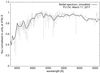 |
Fig. A.1. Comparison of the smoothed model spectrum (the continuous line) and the flux-calibrated and de-reddened FU Ori spectrum (the broken line) obtained on March 11, 2017, three years after our photometric campaign. |
Appendix B:
Model calibration and validation
Before we can carry out a serious application of this model we first need to calibrate and validate it. First, we estimated the zero points necessary for proper calculation of colour indices. For this purpose we used PHOENIX’s emerging intensity of a main sequence A0V star (9600 K, log g = 4.0, μ = 1) and the linear limb-darkening law. Obviously, the disc light was ignored during these calculations. The synthetic fluxes of the star in Johnson–Cousins filters were then properly added to meet the well-known requirement that colour indices of an A0V unreddened star are equal to almost zero.
In the second step, we made an estimate of the interstellar extinction to check whether the results obtained with zero points calculated above are in compliance with the historical results. The unreddened colour indices given by our model are as follows:  . Using the Cardelli et al. (1989) Eqs. (1), (3a), and (3b) for the mean RV-dependent extinction law, and assuming E(B − V) ≈ 0.57, estimated on the basis of results obtained from our model and our observations (B − V ≈ 1.29), we obtained AV = 1.77 for RV = 3.1. Integration of the stellar extinction curve over τλft in the respective wavelength ranges leads to the following values: E(U − V) ≈ 1.00, E(V − Rc) ≈ 0.34, E(V − Ic) ≈ 0.73. This in turn leads to the following, model-dependent colour indices: (U − V)m ≈ 2.20, (B − V)m ≈ 1.29, (V − Rc)m ≈ 0.74 and (V − Ic)m ≈ 1.66 mag. All values are in good agreement with the mean values calculated from all multi-colour observations obtained during the MOST run, i.e. 2.121, 1.291, 0.770, and 1.594 mag, respectively (see also in Table 1 for one particular night). The value AV ≈ 1.8 obtained in this work agrees well with estimates of Zhu et al. (2007) at
  and Pueyo et al. (2012) at
  .
.
In Fig. A.1 we show the final test of our model. The observed (Sect. 2.4) and model-synthesised FU Ori spectra were normalised to unity at the maximum, which for both spectra appear to exist near 4792 Å. Because of the large number of spectral lines in our model spectrum we decided to smooth it for easier comparison. The same E(B − V) value as above was assumed during the de-reddening process of the real FU Ori spectrum within the IRAF task deredden. Similarity of both spectra appears to be satisfactory and it practically does not depend on a particular FU Ori spectrum nor the standard star used for the flux calibration. However, one can note systematically lower observed flux in the region of ultraviolet and blue wavelengths. The observed flux appears to be slightly higher at red wavelengths. This suggests that the maximum disc temperature is currently slightly lower than one or two decades ago, when Zhu et al. (2007) performed their observations and should perhaps be updated. This is not an unexpected finding as the disc brightness, as it is now 81 years after the outburst, is constantly decreasing. Nevertheless, we decided to refrain from this task as this small discrepancy may also be caused by systematic errors in our flux calibration procedure.
One of our model imperfections is the inability to reproduce the shapes of the oscillations as observed in Segments I and III; only reproduction of sine-like wave trains as in Segment II is possible. This is likely due to simplified assumptions about the disc inhomogeneity structure. Additional weakness comes with the assumption that stellar atmosphere models closely match properties of the disc atmosphere as well as with the lack of Iλ for temperatures lower than 2300 K, which slightly influences our results obtained from colour-magnitude diagrams utilising near-infrared filters. We have also omitted the rotational broadening of the spectrum due to the Keplerian rotation of the disc as this effect is negligible for spectrum synthesis results in broadband filters.
All Tables
Colour equation coefficients determined for the SAAO UBVRcIc system during the night of January 11–12, 2014.
Synthetic amplitudes in magnitudes predicted for the rotating spotted stellar surface for Johnson–Cousins filters for three selected hotspot temperatures Tspot.
All Figures
|
Fig. 1. First panel: 2013–2014 MOST light curve of FU Ori provided by the pipeline. The standardised SAAO UBVRcIc (filled circles) and aligned MSO BVRI light curves (open circles and crosses) are shown in the second panel. Third panel: averaged SAAO BVRcIc (filled circles) and MSO BVRI (open circles) observations used for correction of the instrumental trend in the original MOST data, as described in Sect. 2.1. The de-trended MOST data are plotted in the same panel. Fourth panel: de-trended MOST data in the form of orbital averages with error bars (σ). |
| In the text | |
|
Fig. 2. New MOST light curve of FU Ori (top panel) and the ground-based U − V, U − B, B − V, V − Rc and V − Ic colour indices (lower panel) in standard magnitudes, with arbitrary offsets indicated. As mentioned in the text, the MSO data (open circles) were aligned to the standardised SAAO data (filled circles) with an accuracy of 0.002 mag. The grey-shaded area determines the approximate boundaries of Segment II data, as defined in Sect. 3. The Segment I data are shown on the left, while the Segment III data are shown on the right. |
| In the text | |
|
Fig. 3. Results of Fourier analysis of ground-based (upper panel) and MOST (lower panel) data in form of the amplitude a(f) vs. the frequency (f) are shown as continuous lines. The amplitude errors, determined from bootstrap sampling, are shown as dots. |
| In the text | |
|
Fig. 4. Wavelet spectrum computed from the 2013–2014 MOST data. Edge effects are present beyond the white broken lines. |
| In the text | |
|
Fig. 5. Short-periodic fragments of 2013 and 2010 MOST light curves. In both cases maxima and minima were localised by eye to about 0.02 d, which leads to the 0.04 d uncertainty of each indicated temporal period P value. Modulations seen at the beginning are marked by “?” as they occurred prior the official start of Segment II. |
| In the text | |
|
Fig. 6. Colour-magnitude diagrams for FU Ori prepared from data obtained during Segments I, II, and III, as defined in Sect. 3.1. |
| In the text | |
|
Fig. 7. Colour-magnitude diagrams for FU Ori specifically prepared for the first and the third Segment, as defined in Sect. 3.1. A linear least-squares weighted fit is shown and the numerical values of slopes with asymptotic standard error(s) in parentheses are given. Pearson correlation coefficients are also shown. |
| In the text | |
|
Fig. 8. Comparison of Segment II of the MOST light curve with UBVRcIcRI data obtained at ground-based observatories. Last panel: V − (U − V) diagram for this segment; the diagram indicates on larger variability amplitude in U- than in V filter. |
| In the text | |
|
Fig. 9. Comparison of observed (circles, the SAAO data only) and synthetic (squares) colour-magnitude diagrams for Segment I. |
| In the text | |
|
Fig. 10. Sample of synthetic light curves in UBVRcIc filters used during the localisation process of Segment II light variations. Most similar amplitudes in BVRcIc filters are obtained for disc inhomogeneities located between 13 and 20 R⊙, but the slightly higher amplitude in the U filter may suggest somewhat closer localisation, from 12 to 15 R⊙. The values used in a given model (ΔT, |
| In the text | |
|
Fig. 11. Picture proposed for a qualitative explanation of the Segment I variability. The lighter semi-ring represents the 16–20 R⊙ disc inhomogeneity in three rotational phases. The disc fluxes calculated for V filter are expressed in greyscales (as defined on respective bars) and are left in temporary model units; they are also slightly affected by limitations of our plotting software. The stellar flux is expressed arbitrarily; the stellar radius was set to 1.5 R⊙. |
| In the text | |
|
Fig. A.1. Comparison of the smoothed model spectrum (the continuous line) and the flux-calibrated and de-reddened FU Ori spectrum (the broken line) obtained on March 11, 2017, three years after our photometric campaign. |
| In the text | |
Current usage metrics show cumulative count of Article Views (full-text article views including HTML views, PDF and ePub downloads, according to the available data) and Abstracts Views on Vision4Press platform.
Data correspond to usage on the plateform after 2015. The current usage metrics is available 48-96 hours after online publication and is updated daily on week days.
Initial download of the metrics may take a while.