| Issue |
A&A
Volume 618, October 2018
|
|
|---|---|---|
| Article Number | A87 | |
| Number of page(s) | 16 | |
| Section | The Sun | |
| DOI | https://doi.org/10.1051/0004-6361/201833048 | |
| Published online | 16 October 2018 | |
Three-dimensional simulations of solar magneto-convection including effects of partial ionization⋆
1
Instituto de Astrofísica de Canarias, 38205 La Laguna, Tenerife, Spain
e-mail: khomenko@iac.es
2
Departamento de Astrofísica, Universidad de La Laguna, 38205 La Laguna, Tenerife, Spain
Received:
19
March
2018
Accepted:
9
July
2018
In recent decades, REALISTIC three-dimensional radiative-magnetohydrodynamic simulations have become the dominant theoretical tool for understanding the complex interactions between the plasma and magnetic field on the Sun. Most of such simulations are based on approximations of magnetohydrodynamics, without directly considering the consequences of the very low degree of ionization of the solar plasma in the photosphere and bottom chromosphere. The presence of a large amount of neutrals leads to a partial decoupling of the plasma and magnetic field. As a consequence, a series of non-ideal effects, i.e., the ambipolar diffusion, Hall effect, and battery effect, arise. The ambipolar effect is the dominant in the solar chromosphere. We report on the first three-dimensional realistic simulations of magneto-convection including ambipolar diffusion and battery effects. The simulations are carried out using the newly developed MANCHA3Dcode. Our results reveal that ambipolar diffusion causes measurable effects on the amplitudes of waves excited by convection in the simulations, on the absorption of Poynting flux and heating, and on the formation of chromospheric structures. We provide a low limit on the chromospheric temperature increase owing to the ambipolar effect using the simulations with battery-excited dynamo fields.
Key words: Sun: photosphere / Sun: chromosphere / Sun: magnetic fields / methods: numerical
The movies associated to Figs. 16 and 17 are available at https://www.aanda.org
© ESO 2018
1. Introduction
The solar chromosphere is a boundary layer between the interior and exterior of the Sun. The plasma in the solar photosphere and chromosphere is only partially ionized. In the past few years it has been repeatedly demonstrated that processes related to non-ideal plasma behavior due to the presence of a neutral plasma component may be key to solving the problem of chromospheric heating, dynamics, and fine structure (De Pontieu & Haerendel 1998; Goodman 2000, 2011; Judge 2008; Krasnoselskikh et al. 2010; Goodman & Kazeminezhad 2010; Song & Vasyliūnas 2011; Martínez-Sykora et al. 2012; Khomenko & Collados 2012a; Shelyag et al. 2016).
The chromosphere hosts shock waves and current layers. Magnetic field lines, rooted in the photosphere, are constantly perturbed by convective plasma motions, which serve as an energy reservoir. A significant part of energy of these motions is transported to the chromosphere in the form of various types of waves. However, not all wave types are able to reach and deposit their energy at the chromosphere. According to the mode conversion theory (Cally 2006; Cally & Goossens 2008), acoustic p-modes propagating in subsurface layers can be transformed into fast magneto-acoustic and Alfvén waves when reaching the magnetically dominated layers higher up. Alfvén waves created by this mechanism might be able to reach the chromosphere more easily. This mode transformation mechanism is confirmed by numerical simulations (Khomenko & Collados 2006; Khomenko & Cally 2012; Felipe 2012) and is recognized to be responsible for the formation of high-frequency acoustic halos surrounding active regions (Khomenko & Collados 2012a; Rijs et al. 2015, 2016).
Magnetic waves reaching the chromosphere may create perturbations in magnetic field, i.e., produce perturbations of currents. These currents can be dissipated via either classical Ohmic diffusion or ambipolar diffusion, related to the presence of neutrals. At chromospheric layers, as a consequence of incomplete collisional coupling, ions would move under the action of the magnetic Lorentz force and would be constantly disrupted by neutrals that do not sense this force directly, but only through collisions with ions. The magnetic field frozen in the charged plasma component would diffuse because of this differential motion between ions and neutrals. This friction creates dissipation and therefore makes it possible to transform magnetic energy into heat. Mathematically, when the single-fluid approximation is adopted, the above effect results in large ambipolar diffusion coefficients (Khomenko & Collados 2012a; Khomenko et al. 2014a) and the internal energy of the plasma would increase proportional to  . The ambipolar diffusion effect removes currents perpendicular to the magnetic field, approaching a force-free field in the relaxed state (Leake & Arber 2006; Arber et al. 2007).
The dissipation of static currents at the borders of chromospheric flux tubes has been shown to be efficient to balance the radiative losses of the chromosphere (Khomenko & Collados 2012a,b). However, currents created dynamically by waves and motions are found to be even more effective. There are theoretical works and idealized numerical simulations suggesting that dissipation of Alfvén waves due to effects of ion-neutral interactions is an important source of chromospheric heating (Goodman 2000, 2011; Shelyag et al. 2016,among the recent ones). In particular, Goodman (2000) concluded that the chromosphere is heated by flux tubes with photospheric magnetic field strength between 700 and 1500 G. Shelyag et al. (2016) considered a more complete model where acoustic waves were generated outside of a magnetic flux tube, then entered the flux tube, and double converted into the fast magnetic waves and then into Alfvén waves. In their example up to 80% of the magnetic Poynting flux of waves could be absorbed and converted to heat. In a continuation of this work Przybylski et al. (2018) demonstrated that this absorption depends non-trivially on the frequency and is a highly non-linear process in which the amount of absorption depends on the wave amplitude. Other studies concluded that compressible dissipation in shocks is as efficient (or more) as dissipation due to the ambipolar diffusion mechanism (Goodman & Kazeminezhad 2010; Arber et al. 2016).
Realistic numerical simulations are a necessary next step to provide quantitative conclusions about the importance of neutrals in the chromospheric energy balance and to evaluate the role of other mechanisms mentioned above, such as shocks. Realistic two-dimensional numerical simulations including ambipolar diffusion have been employed by Martínez-Sykora et al. (2012, 2016, 2017). Martínez-Sykora et al. (2012) showed that the temperature in cool chromospheric bubbles produced during the nearly adiabatic expansion of the material reaching upper layers does not drop to such low values as in the models without ambipolar diffusion. Martínez-Sykora et al. (2016, Martínez-Sykora et al. 2017) claimed that spicules can be produced from the effects of ambipolar diffusion by allowing the field lines to reach higher, and that chromospheric fibrils and the magnetic field can become visibly misaligned from the same effect. Apart from wave fronts, vortex motions have been recently identified as another mechanism of energy transport to the upper layers (Moll et al. 2011, 2012; Wedemeyer-Böhm et al. 2012; Shelyag et al. 2013; Kitiashvili et al. 2013; Wedemeyer & Steiner 2014). When three-dimensional simulations of magneto-convection are employed, it has been shown that vortices are formed differently and have different properties in non-magnetized and magnetized areas. Those in magnetized areas reach higher and can act as channels energetically connecting the photosphere and chromosphere.
The aim of the present work is to advance the investigation of ion-neutral effects on the energy balance of the solar chromosphere. To that aim, we have performed three-dimensional simulations of dynamo and magneto-convection including the effect of ambipolar diffusion (as a main non-ideal effect) using the generalized Ohm’s law. We statistically compare pairs of simulation runs with and without ambipolar diffusion. Results regarding the Poynting flux absorption as a function of frequency and magnetic structure are presented. We also study the formation of fine structures. The effects on the average chromospheric temperature increase are discussed.
2. Magneto-convection simulations by MANCHA3D
The simulations presented in this paper were carried out with the MANCHA3D code (Khomenko & Collados 2006; Felipe et al. 2010; González-Morales et al. 2018). MANCHA3Dsolves the non-ideal non-linear equations of single-fluid MHD, in which equilibrium is explicitly removed from the equations. The code treats the most important effects derived from the presence of neutral atoms in the solar plasma. These effects are ambipolar diffusion, the Hall effect, and battery effect (Khomenko & Collados 2012b), assuming that plasma is strongly colisionally coupled. In this approximation, well justified in the photosphere and low chromosphere, the non-ideal effects manifest themselves through additional terms in the generalized induction equation with the corresponding repercussion on the energy conservation equation (Eqs. (3) and (4) below), see Khomenko et al. (2014b) and Ballester et al. (2018). The numerical treatment of these terms is described in González-Morales et al. (2018).
In this work we neglect the Hall effect and therefore the only two non-ideal effects treated in this study are ambipolar diffusion and the battery effect. The following equations are solved in the code: (1)
(1)
![$ \begin{aligned}&\frac{\partial {\rho \mathbf{v }}}{\partial {t}}+ \mathbf{\nabla }\cdot \left[\rho \mathbf{v } \mathbf{v } + \left( p_{1} + \frac{\mathbf{B }_{1}^{2} + 2\mathbf{B }_{1} \cdot \mathbf{B }_{0}}{2 {\mu }_{0}} \right) \mathbf{I } \right]\nonumber \\&\quad \quad \quad \quad \,+\,\mathbf{\nabla }\cdot \left[\frac{1}{{\mu }_{0}} \left(\mathbf{B }_{0} \mathbf{B }_{1}-\mathbf{B }_{1} \mathbf{B }_{0}-\mathbf{B }_{1} \mathbf{B }_{1} \right) \right] \nonumber \\& \quad \quad \quad = \rho _{1} \mathbf g + \left(\frac{\partial {\rho \mathbf{v }}}{\partial {t}}\right)_{\mathrm{diff}}, \end{aligned} $](/articles/aa/full_html/2018/10/aa33048-18/aa33048-18-eq3.gif) (2)
(2)
![$ \begin{aligned} \frac{\partial {\mathbf{B }_{1}}}{\partial {t}}= \mathbf{\nabla } \times \left[\mathbf{v } \times \mathbf{B } + \frac{\mathbf{\nabla }p_{\mathrm{e}}}{e n_{\mathrm{e}}} + \frac{\left(\eta _{\mathrm{A}}\mathbf{J } \times \mathbf{B } \right) \times \mathbf{B } }{|B|^{2}} \right] + \left(\frac{\partial {B_{1}}}{\partial {t}}\right)_{\mathrm{diff}}, \end{aligned} $](/articles/aa/full_html/2018/10/aa33048-18/aa33048-18-eq4.gif) (3)
(3)
![$ \begin{aligned}&\frac{\partial {e_{1}}}{\partial {t}} + \nabla \cdot \left[ \mathbf{v }\left(e + p + \frac{|\mathbf{B }|^{2}}{2 \mu _0} \right) - \frac{\mathbf{B }(\mathbf{v } \cdot \mathbf{B }) }{\mu _0} \right] \nonumber \\&\quad = \rho \left(\mathbf g \cdot \mathbf{v }\right) + \mathbf{\nabla }\cdot \left[ \frac{\mathbf{B } \times (\eta _{\mathrm{A}} \mathbf J_\perp ) }{\mu _0} + \frac{\mathbf{\nabla }p_{\mathrm{e}} \times \mathbf{B }}{e n_{\mathrm{e}} \mu _0}\right] \nonumber \\&\quad \quad \,+\,Q_{\mathrm{R}} + \left( \frac{\partial {e_{1}}}{\partial {t}}\right)_{\mathrm{diff}}, \end{aligned} $](/articles/aa/full_html/2018/10/aa33048-18/aa33048-18-eq5.gif) (4)
(4)
where generally, ρ = ρ0 + ρ1, p = p0 + p1, B = B0 + B1, v = v1, and e = e0 + e1 = ( ρ0 + ρ1)v2/2 + (B0 + B1)2/2/μ0 + (eint0 + eint1) is the total energy. In the code we have freedom to set variables as background (index “0”) or perturbation (index “1”); the only requirement is that the background variables fulfill the condition of (M)HS equilibrium. In the experiments performed in this work the initial equilibrium was chosen to be purely hydrostatic, such that B0 = 0 and the entire magnetic field vector is contained in the variable B1. The terms subscripted with “diff” are numerical diffusion terms required for numerical stability. These terms are computed according to Vögler et al. (2005) and Felipe et al. (2010); see also the detailed description in the PhD Thesis of A. Vögler1.
The ambipolar diffusion coefficient is calculated in units of [ml3/tq2] according to the following expression: (5)
(5)
where the collisional parameter αn is defined as (6)
(6)
and the summation covers all available chemical species of neutrals and singly ionized ions. The collisional frequencies νe; bn, νai; bn are defined in Braginskii (1965), Draine (1986), Lifschitz (1989) and Rozhansky & Tsedin (2001); see also the review by Ballester et al. (2018).
The system of equations is closed with an equation of state (EOS) for the solar chemical mixture given by Anders & Grevesse (1989). The internal energy (eint), density ( ρ), and electron pressure (pe) are precomputed for a temperature (T) – pressure (p) grid following the algorithm of Mihalas (1967) based on the Saha equation. The EOS takes into account the effects of the first and second atomic ionization for all included elements (Z ≤ 92), and formation of hydrogen molecules. The ionization fraction is obtained self-consistently with the rest of thermodynamical variables providing all necessary variables to compute the neutral fraction, ξn = ρn/ρ and the ambipolar diffusion coefficient via Eq. (5). The EOS results are stored in lookup tables giving efficient conversion method between thermodynamic quantities and a possibility to use different EOS realization (with different chemical composition or including non-ideal terms such as electron degeneracy and pressure ionization) that are relevant for other simulations stretching deeper into the convection zone.
The radiative loss term QR is computed by solving the non-gray radiative transfer (RT) equation, assuming local thermodynamic equilibrium (LTE), using domain decomposition, as in Vögler et al. (2005). The wavelength dependence of the emission and absorption coefficients is discretized using the opacity binning method (Nordlund 1982). In the runs considered in this paper we used one single bin, i.e., the so-called gray approximation. The angle integration is done using quadrature with three rays per octant. The formal solver used in the RT module is based on the short-characteristics method by Olson & Kunasz (1987). The LTE approximation limits the accuracy of the RT module in simulations extending above the photosphere. In the optically thin corona, the code uses Newtonian cooling approximation. Nevertheless, keeping these limitations in mind, we computed models extending somewhat higher to the lower chromosphere, reaching approximately 1400 km above the solar surface, as detailed in the section below.
2.1. Details of the runs
We discuss four runs of magneto-convection simulations. To initiate the convection we started with a plane-parallel atmosphere that combines a model of solar convection zone by Spruit (1974) below the surface with the Harvard Smithsonian Reference atmosphere (HSRA) model (Gingerich et al. 1971) above the surface. The two models are joined in a smooth way imposing the hydrostatic equilibrium and consistency with the EOS used in the code. The box size is 5.8 × 5.8 × 2.35 Mm3 covered by 288 × 288 × 168 uniformly distributed grid points, i.e., with a horizontal sampling of 20 km and vertical sampling of 14 km. The height range includes approximately 0.95 Mm below the surface and about 1.4 Mm above the surface. Random noise was introduced to the internal energy to initiate the instability. The horizontal boundaries are periodic and the upper boundary is closed for mass flows. We set symmetric boundary conditions (zero gradient) in internal energy and density variables at the top boundary and the temperature is computed through the EOS. We do not set any specific condition to keep the temperature at a given value at the top boundary, allowing shock viscous dissipation, magnetic field related mechanisms, and radiative losses to set the structure of the atmosphere. The bottom boundary is open for the mass flow with automated control of the fluctuation of the total mass and total radiative output (similar to, Vögler et al. 2005) and with zero magnetic field inflow. This way the simulation maintains a required value of outgoing flux and keeps approximately constant the mass of the domain.
The initial equilibrium atmosphere is set in a way that the outgoing flux is equal to the mean solar value of 6.3 × 10⁷ J m−2 s−1. Since convection is not initially developed, it does not provide convective energy transport and there is only energy transport by radiation. Therefore, at the beginning of the simulation, the outgoing flux starts to decrease reaching a minimum of about 2.3 × 10⁷ J m−2 s−1 after about 9 min of solar time. The mean temperature in the simulation box, given by T = T0 + T1 drops down in this initial phase. At this stage, convection is developed enough and becomes efficient channel for energy transport. Also, the downflowing material has already reached the lower boundary. Altogether, convection leads to a smooth recovery of the value of the outgoing flux back to the solar value and also results in a temperature increase. In total, this initial phase takes about 20 min of solar time. We then run the purely hydrodynamical (HD) convection for another 3.4 h of solar time to make sure it reached a stationary regime.
At this point we take a snapshot of stationary HD convection and perform one of the following actions: first, switch on the battery term in Eqs. (3) and (4), and second, introduce a constant vertical unipolar field of 10 G strength into the simulation box. We refer to the first case as a dynamo (D) run and to the second case as unipolar (U) run.
The battery term in the D run generates the small-scale dynamo seeds with a strength of 10−6 G; see Khomenko et al. (2017). Its continuous action, together with dynamo amplification, provides the magnetization of the model with ∼102 G mean field strength at the τ5 = 1 surface, after reaching the saturated regime in about 2 h of solar time (see Fig. 3 in Khomenko et al. 2017). We run D simulation for 4.2 h of solar time in total after switching on the battery term with about 2 h in the stationary saturated dynamo regime.
In the U run, the field is quickly moved into intergranular lanes through flux expulsion, where it forms kG concentrations, as seen many times in the simulations reported in the literature (see, e.g., Vögler et al. 2005). We let the U simulation run for 82 min of solar time to reach a new stationary state.
Finally, we take a snapshot of either (1) stationary dynamo (D) run or (2) stationary unipolar (U) magneto-convection run, and switch on the ambipolar term (referred as AD later) in Eqs. (3) and (4). We then let the D simulation run for another 150 min of solar time with the ambipolar diffusion term on. During the last 50 min we saved snapshots every 20 s and used these for the analysis in the current paper. We label this simulation as D-AD; see Table 1. Similarly, we let the U simulation run 206 min with AD on, and saved snapshots every 20 s during the last 50 min. This simulation is labeled as U-AD; see Table 1.
In parallel, we kept running D and U simulations with exactly the same setup but with ambipolar diffusion switched off (D-noAD and U-noAD from Table 1). These runs are used for comparison purposes. Since our RT losses calculation for the chromosphere include several approximations (as LTE), we cannot make conclusions about the average temperature structure in the chromosphere from such runs. We rather do a statistical comparison between the temperature and other parameters in the runs with and without ambipolar diffusion.
The MANCHA3Dcode uses temperature fix based on internal energy to prevent the temperature in the domain from going below a certain limit (about 2000 K). The temperature in the D-AD run needs to be fixed in 0.0045% of points, while in the D-noAD run it is in 0.0057% of points. In the U runs the percentage of points to fix is similar in the AD and noAD case, 0.0004%.
Parameters of the simulation runs.
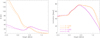 |
Fig. 1. Left panel: time- and space-averaged modulus of the magnetic field strength as a function of height in the four simulation runs. Right panel: time- and space-averaged magnetic field inclinations with respect to the vertical direction. Orange solid: D-AD; orange dashed: D-noAD; violet solid: U-AD; violet dashed: U-noAD. The time averaging interval is 50 min. |
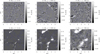 |
Fig. 2. Vertical magnetic field at three selected heights for a snapshot of the D-AD run (upper row) and U-AD run (bottom row). The heights are indicated at the title of each panel. Notice the complex structure of fields in the D run, and the expansion of the magnetic field structures with height in both runs. Contours indicate the locations with zero vertical velocity at z = 0, highlighting the structure of granulation. The horizontal black line marks the location of cuts shown in Fig. 3 below. |
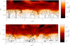 |
Fig. 3. Cuts through the simulation snapshots over horizontal x and vertical z directions. The locations of the cuts are marked in Fig. 2. The color image shows the temperature. The black lines are the projections of the magnetic field lines into the x − z plane. Only the field lines with the average field strength above 5 G are drawn. Top panel: D-AD run; bottom panel: U-AD run. |
2.2. Global properties of the simulations
The resulting distributions of the time-averaged magnetic field strength and inclination with height in all four runs are shown in Fig. 1. In the D runs (orange solid and dashed lines), the field smoothly decreases its strength with height from hG values below the photosphere to a few G in the chromosphere and has a secondary maximum around 0.5 Mm in the photosphere. This maximum is produced by strongly inclined fields, connecting complex bipolar structures produced in these simulations; see Fig. 3 and the corresponding discussion later on. The average inclination of the field in the D runs, shown at the right panel of Fig. 1 (orange curve), reflects this behavior. The field is on average more vertical at heights below the photosphere (average inclinations around 40–5°). Between about 0.2 and 1 Mm, the average inclination is 70–80°. The field strength becomes extremely weak in the D-runs above 1 Mm, and its inclination tends to the vertical again, imposed by the boundary condition in our simulations. In the U run, a similar tendency is observed with the field decreasing with height and with a more pronounced secondary maximum (violet solid and dashed lines in Fig. 1). The mean field in the U simulations is lower than in the D simulations in the subsurface layers and in the photosphere, but is larger in the chromosphere. This happens because more chaotic and complex fields produced in the dynamo simulations are connected and form loops at lower heights, compared to the relatively unipolar U runs. The field expands with height and becomes more horizontal in the U runs around 0.4–0.5 Mm (inclinations close to 80° in Fig. 1, right panel), but then it quickly becomes vertical again. The comparison between AD and noAD runs reveals that the mean field strength is slightly lower in noAD runs in the subsurface layers and in the low photosphere. In the chromosphere, the mean B in noAD run is higher than in the AD run for the dynamo simulations and there is no appreciable difference for the unipolar simulations.
The horizontal distribution of the vertical magnetic field component is shown in Fig. 2 for the D-AD and U-AD runs. As expected, the field has an extremely complex structuring in the D-AD run with an almost balanced mixture of positive and negative polarities. The magnetic structures are mostly rooted in intergranular lanes at photospheric level (z = 0 km) and are expanding with height. This expansion is more evident in the U runs. In the D runs, it is possible to observe the expansion comparing the field maps at 0 and 488 height (left and middle image in Fig. 2, top). At the lower chromosphere (z = 728 km) a layer of strongly inclined canopies is produced in both simulations. These canopies are evident from the rightmost panels of Fig. 2 by the presence of the fields filling a large amount of space, and not only intergranular zones, as in the photosphere. The differences in the overall structure of the field in both types of simulations are better visualized in Fig. 3, by showing the projections of the magnetic field lines in the x − z plane for the D-AD (top) and U-AD (bottom) simulation runs. The field lines form a layer of strongly inclined fields in the upper photosphere and connect at relatively low heights in the D-AD run. The field is mostly weak and horizontal at chromospheric heights. Unlike that, the field is extending into higher layers in the U-AD run and is more aligned with the vertical direction, forming classical flux-tube-like expanding structures.
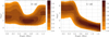 |
Fig. 4. Bidimensional histogram showing the number of occurrences of a given value of plasma β as a function of height in D-AD run (left panel) and U-AD run (right panel). Darker colors mean larger probability of occurrence in logaritmic scale, indicated by the color bar. |
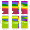 |
Fig. 5. Top panels: power spectra of flong (left), ffast (middle) and falf (right) as a function of height and frequency for the D-AD run. For better visualization, the maps are scaled with a factor ρ0, the density of the unperturbed atmosphere. Bottom panels: ratio of D-AD to D-noAD power maps. The power is shown in log 10 units of J m−5 Hz−1. |
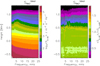 |
Fig. 6. Amplitude spectra of the vertical component of the Poynting flux, |

3. Statistical Fourier analysis
The patterns of convection and magnetic field distribution developed in the AD and noAD runs are different. Therefore their properties can only be compared in a statistical way. Below we perform a statistical analysis of various aspects of the simulations. We are primarily interested in the properties of waves generated in the simulations, and their dissipation at chromospheric heights. We also compare the amount of heating and thermal properties of the D and U simulations.
Convective motions, similar to any turbulent flow, generate waves. The generation of waves in convection simulations have been studied elsewhere (Stein & Nordlund 2001; Nordlund & Stein 2001). The high cadence and length of our simulated series allows us to study waves up to high frequencies. The wave properties are intrinsically related to the strength and topology of the magnetic field configuration in the medium in which they propagate. Therefore, to separate different wave modes as much as possible, we base our study on their physical properties and construct quantities serving as proxies for these modes. In a horizontally homogeneous plasma and in the cold plasma approximation, when no acoustic modes exist, Cally (2017) separated the fast magnetic and the Alfvén modes by calculating the divergence and curl of the wave velocity, correspondingly. This works well because the Alfvén mode is incompressible, and the only mode involving compressibility is the fast magnetic mode. In a warm and horizontally structured plasma, there are at least three wave modes to deal with (fast and slow magneto-acoustic and Alfvén), keeping in mind that none of these are pure modes as in a homogeneous plasma. In order to maximize the separation between these modes, we follow the strategy in Cally (2017) and construct the following quantities: (7)
(7)
 (8)
(8)
 (9)
(9)
We note that the quantities defined by Eqs. (7)–(9) are not velocities but their derivatives. Here, υ‖ = ê‖ ∙ v and v⊥ = v − ê‖υ‖ are the velocity components parallel and perpendicular to the magnetic field, and ê‖ is the field-aligned unit vector. A similar approach was also used by Przybylski et al. (2018) in a simpler situation for the study of waves in an isolated expanding flux tube, showing good results. Independent of the plasma β, falf gives an incompressible perturbation propagating along the field lines and separates the Alfvén waves. The quantity flong gives the compressible perturbation propagating along the field lines, and separates the slow mode (essentially acoustic) waves in β < 1. The remaining quantity, ffast gives the compressible perturbation in the direction perpendicular to the field lines, separating the fast mode (essentially magnetic) waves for β < 1.
The plasma β in the simulations vary strongly as a function of the spatial coordinates and time, depending on the evolution of magnetic structures. The bidimensional histograms of the plasma β as a function of height are given in Fig. 4. It can be seen that, for the weakest fields in the D runs, the lowest values of β are achieved between 600 and 800 km, and they are almost always above unity. In the U runs, a progressively larger part of the domain contains plasma with β < 1 starting from approximately 600 km height.
We constructed power maps of falf, ffast, and flong as a function of height and frequency. For that, we computed the temporal power spectra of these quantities at each spatial point and at every height. The spectra were then averaged over the two horizontal directions. These power maps are shown in Figs. 5 and 7 for D and U simulations, correspondingly.
We also consider the Poynting flux reaching the upper levels of the simulation domain. The total energy conservation equation can be rewritten in terms of the electro-magnetic Poynting flux as follows: (10)
(10)
where we removed the small artificial diffusivity term of Eq. (4), and have used the expression for the radiative flux, QR = −∇FR. The electromagnetic Poynting flux is defined as (11)
(11)
The contribution from the battery term to SEM is expected to be small, and the main difference between simulations with/without AD is expected to come from the presence of the ambipolar term, which is the first term on the right hand side of Eq. (11). Therefore, we neglect the contribution of the battery term and split SEM into ideal and ambipolar parts as (12)
(12)
The Fourier amplitude maps of the vertical component of the ideal part of the Poynting flux,  , are shown in Figs. 6 and 8 for the D and U simulations, correspondingly.
Before proceeding with the description of the results, it is interesting to check which velocities create the ideal part of the Poynting flux in the U and D simulations. For that we split  into horizontal and vertical parts, following Shelyag et al. (2012),
 (15)
(15)
 (16)
(16)
The horizontal part corresponds to horizontal motions along vertical flux tubes, while the vertical part corresponds to horizontal magnetic field perturbations transported by vertical plasma motions. In their paper, Shelyag et al. (2012) concluded that torsional motions in the magnetic flux tubes produce most of the ideal Poynting flux, i.e.,  , while earlier Steiner et al. (2008) claimed that the largest part of this flux is due to the vertical motions and magnetic field advection, i.e., the opposite is true. In our case, we get that for D simulations,
  is about an order of magnitude smaller than
  , similar to the results by Shelyag et al. (2012). In the U simulations the situation is not so straightforward. We obtain that
  below the surface and they are similar above the surface. This is an interesting behavior and will need a future detailed study.
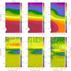 |
Fig. 7. Top panels: power spectra of flong (left), ffast (middle), and falf (right) as a function of height and frequency for the U-AD run. For better visualization, the maps are scaled with a factor ρ0, which is the density of the unperturbed atmosphere. Bottom panels: ratio of U-AD to U-noAD power maps. The power is shown in log 10 units of J m−5 Hz−1. |
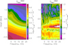 |
Fig. 8. Amplitude spectra of the vertical component of the Poynting flux, |

3.1. D runs
Figure 5 shows the power maps of the quantities defined by Eqs. (7)–(9) for the D-AD run (top), and the ratio of the D-AD to D-noAD power maps (bottom). We do not show the maps for the D-noAD case, since the differences from the D-AD maps cannot be appreciated well because of the logarithmic change of the power with height.
The power maps show the spectrum characteristic for convective motions below the photosphere (negative heights). There is hardly any difference in power between the D-AD and D-noAD cases for heights below 0 km; see the bottom panels of Fig. 5 (green colors marking values close to 1). The power distributions for flong, ffast, and falf show most differences in the atmospheric layers, where the magnetic field has an increasing influence.
The power maps of the flong and ffast look rather similar to each other. This is not surprising since both quantities select compressible waves, and the values of the plasma β in the D-AD run are not low enough to provide anisotropy in the compressible wave propagation along and across the magnetic field. The power of flong and ffast in the atmospheric layers reveals a spectrum that is typical for the solar 5 min oscillations with a broad maximum between 2 and 10 mHz. The length of the simulated series (40 min) does not allow us to resolve individual power peaks well. Still, the power maps ratios (left and middle bottom panels) show discrete vertical strips pattern at frequencies between 2 and 10 mHz, reflecting slight differences between power peaks locations in the D-AD and D-noAD runs, probably caused by differences in their average temperature structures.
The spectrum of the falf quantity (top right panel of Fig. 5) is different from that of flong and ffast, showing more power at low frequencies. The dominance of Alfvén waves (selected by the falf quantity) in the middle photosphere above 500 km can be explained by the presence of the layer with strongly inclined fields in the simulations at those heights (see Figs. 1 and 3), which produce favorable conditions for the fast to Alfvén mode transformation (Cally & Goossens 2008; Khomenko & Cally 2012).
The ratio of the power maps to the f-quantities, shown in the bottom panels of Fig. 5, tells us about the differences in the amount of wave energy present at a given height and at a given frequency, depending on whether the ambipolar term is operating or not. The power ratio maps remarkably show the presence of power depression layers, where the power of waves in the D-AD simulations is decreased compared to that of the D-noAD simulations; see the violet-purple-black strips at the bottom panels of Fig. 5. This decrease reaches up to 30–40% for the falf quantity. The location and extension of the power depression layers depends on the f-quantity and on the wave frequency. It is interesting to note that the depression is not a smooth function of frequency in any of the cases. Both flong and ffast have a power depression layer located between 400 and 800 km, roughly coinciding with the heights in which strongly inclined fields exist in the D-AD and D-noAD simulations (see Figs. 1 and 3). The height coverage (width) of the depression layer increases with increasing frequency. The strength of the depression also increases with frequency. There is a secondary power depression layer located higher up above 1.2 Mm as well.
It is remarkable that the power depression is significantly stronger for the falf quantity, representing incompressible perturbations. In the power depression layer located between 400 and 800 km, the amount of depression increases toward the high frequencies. In the secondary power depression layer located above 1 Mm, this behavior reverses; the amount of depression decreases with frequency, being largest for incompressible waves with the lowest frequencies.
There can be several alternative explanations for the power distributions. On the one hand, the structure of the field can be different in the D-AD and D-noAD simulations owing to the proper effect of the ambipolar diffusion on the field. In the AD simulations the field may reach higher heights by diffusing through the neutral chromospheric layers, as in Leake & Arber (2006) and Arber et al. (2007). This may displace the regions with maximum wave power at a given frequency to a different layer. On the other hand, the change of the average field structure can affect the mode transformation process, making the relative weight between the various wave modes change with height and frequency in a different way for the D-AD and D-noAD simulations. The efficiency of the mode transformation could also be affected directly by the presence of the ambipolar diffusion; see the recent study by Cally & Khomenko (2018).
Apart from the possible change in the average field structure and efficiency of the mode transformation process, real physical absorption and wave power conversion into heat can be taking place. Wave absorption due to dissipation of the ambipolar currents was studied recently by Shelyag et al. (2016) using idealized simulations of wave propagation in isolated flux tubes. There, waves at a single frequency of 25 mHz were studied. While the structure of the field was significantly different in the simulations by Shelyag et al. (2016), it is interesting that a similar effect is now confirmed in a more complex and realistic situation. Additionally, a similar non-smooth behavior of the wave power depression with frequency was found by Przybylski et al. (2018) in a work continuing the initial results by Shelyag et al. (2016). Fully understanding these effects would require more idealized simulations to be carried out. In particular, unlike in idealized cases, we observe a significant power depression for the longitudinal component of the velocity. This peculiarity may have to do with the particular field structure in the current simulation run (see next section).
The Poynting flux tells us about the propagation of wave energy, and not only about its amount at a given height. To check if there is physical absorption of the wave energy, Fig. 6 shows amplitude maps of the vertical component of the ideal part of the Poynting flux vector, Eq. (14). Similar to the velocity power maps, the Poynting flux in the deep layers is essentially the same in the D-AD and D-noAD runs (see the green colors of the right panel). It also shows the presence of a broad power maximum for frequencies characteristic for solar waves between 3 and 10 mHz above the surface. The most prominent feature, however, is the strong decrease of the SEM in the D-AD simulation compared to the D-noAD simulation in the upper layers. The absorption of the flux reaches up to 80–90% in the uppermost part of the simulation domain, being higher for lower frequencies. The amount of Poynting flux absorption coefficient agrees well with that reported by Shelyag et al. (2016) from idealized simulations.
3.2. U runs
The magnetic field is mostly unipolar in the U runs. Because of the granular motion, most of the magnetic field is moved into the intergranular lanes where it forms nearly vertical expanding flux tubes with a photospheric strength close to kG values; see Figs. 2 and 3. The average field strength in the atmospheric layers is larger in the U simulations compared to the D simulations; see Fig. 1. Because of this more regular and generally less chaotic field topology, the combination of wave modes developed in the U simulations is different to that of the D simulations. The power maps of the f-quantities, given in Fig. 7, reflect these changes.
Similar to the D runs, the power maps of the flong and ffast quantities show a broad power peak in the atmospheric layers between 2 and 10 mHz, characteristic for solar 5 min oscillations (upper left and middle panels). The spectrum of the flong (upper right) provides a smoother decrease of the power with frequency and an enhanced presence of low-frequency waves.
The most significant difference, however is in the power depression maps shown at the bottom panels of Fig. 7. Unlike the D runs, the amount of power depression is significantly less (10–15%) and there is no secondary depression band above 1 Mm for the flong and ffast quantities. In fact, the power of compressible waves, selected by flong and ffast, in the U-AD simulations is up to 20–25% higher above 0.5 Mm compared to the U-noAD case. The amount of power depression is still a function of frequency and it is increasing for higher frequencies.
The power ratio maps for the incompressible waves, selected by falf (bottom right) show a secondary extended power depression band above 800 km, where the maximum value of depression is still below 15%. There is about 20% power enhancement for highest frequencies at heights around 400 km.
Since the ambipolar diffusion coefficient, Eq. (5), is proportional to the magnetic field strength squared, one could intuitively expect that the wave dissipation should be larger in models with average larger field strengths, as we have in the U runs. However, our simulations show the opposite results. This brings us to the conclusion that the efficiency of the wave power absorption via AD mechanism is intimately related to the magnetic field structure. The eventual efficiency of the energy transfer will not only depend on the strength of ηA, but also on the strength and abundance of perpendicular currents to dissipate. The more chaotic and bi-polar field structures developed in the D simulations apparently provide a better source of perpendicular currents than the more regular and unipolar fields in the U runs.
The amplitude maps of the Poynting flux, shown in Fig. 8, confirm this conclusion. We observe that the Poynting flux contributes less at high frequencies in the U runs, compared to the D runs. There is a layer above 0.5 Mm in which the absorption due to the AD mechanism is present. However, the amount of absorption is significantly less in the U case, with up to 30%, compared to 90% in the D runs. There is also a layer around 0–0.2 Mm in which the Poynting flux in the U-AD case is about 50% larger compared to the U-noAD case (orange-red-white strip). The origin of this strip should be investigated further.
It is important to underline the difference between the power ratio maps of the f-quantities (bottom panels of Fig. 7) and the amplitude ratio map of the Poynting flux (right panel of Fig. 8). The locations of the strips in which the amount of the available kinetic energy is less in the U-AD runs compared to U-noAD runs do not coincide with the location of the strip in which the Poynting flux is absorbed, except for the upper depression band for falf. This happens because the quantities studied are fundamentally different. While the power maps in Fig. 7 indicate the amount of kinetic energy available, the Poynting flux indicates the amount of electromagnetic energy that propagates through the region. For example, the wave energy cannot propagate for waves that are evanescent, standing, or trapped by some mechanism; even if their ρv2 is large, their energy flux might be zero. The Poynting flux absorption maps, as in Fig. 8, indicate the amount of wave electromagnetic energy physically absorbed in a given layer.
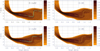 |
Fig. 9. Bidimensional histograms showing the logarithm of the number of points with a given value of temperature at a given height. The darker colors mean larger number of points, indicated at the bar in log10 scale. Upper left panel: D-noAD run; upper right panel: D-AD run; bottom left panel: U-noAD run; bottom right panel: U-AD run. Yellow and light blue lines follow the maximum value of the distribution at each height for AD/noAD runs, correspondingly. |
 |
Fig. 10. Bidimensional histograms showing the logarithm of the number of points with a given value of the heating term, |

4. Heating properties of the simulations
The absorption of Poynting flux allows us to convert wave energy into heat and should eventually be reflected on the average temperature structure in the simulations. Since we only have a simplified treatment of RT, using LTE in the chromospheric layers, we can only extract conclusions about the average temperature increase by comparing the AD and noAD cases statistically. Figure 9 shows bidimensional histograms of the temperature distribution as a function of height in the four simulation runs. The histograms include all spatial points and the whole temporal series duration. The figure only shows the height range from the photosphere upward where the difference due to the presence of the AD effect is expected to be important. While in general the temperature stratifications between the AD and noAD cases seem rather similar, there are also significant differences. The upper right panel of Fig. 9 demonstrates that there are more locations with higher chromospheric temperatures (heights between 0.8 and 1 Mm). The difference between AD and noAD cases is better appreciated by comparing the yellow and light blue curves that follow the maximum value of the distribution at every height. It can be seen that at heights between 0.8 and 1 Mm in the D run (upper panels), the maximum of the distribution is shifted toward 200–300 K higher values for the AD case. On average, the temperatures in the D run are about 50 K larger in the AD case at these heights. However, it should be noted that the temperature distributions at all heights are wide and have a complex shape, such that mean values are not the best quantities to characterize such distributions.
The average temperatures are still slightly larger in the U-AD case compared to the U-noAD case (low panels of Fig. 9), but the effect is significantly smaller than in D cases. In fact, the maximum values of the distribution are larger in the U-noAD case, showing just the opposite effect to the D cases. This can be a consequence of the lower amount of absorbed Poynting flux in the U simulations compared to the D simulations.
Figure 10 shows the histograms of the distribution of the heating term,  , as a function of height in the D-AD (left) and U-AD (right) simulations. The energy conservation equation, Eq. (4), can be rewritten in terms of conservation of internal energy only, by removing the kinetic and magnetic energy parts using the momentum and induction equations,
 (17)
(17)
The right-hand side of this equation contains the Ohmic heating term related to the ambipolar diffusion. This term gives the efficiency of conversion between the magnetic and thermal energies, see Khomenko & Collados (2012a), and is the quantity shown in Fig. 10. The efficiency of the energy conversion depends on the magnitude of the ambipolar diffusion coefficients, but also on the strength of the perpendicular currents, J⊥. While the first one (ηA) is essentially a function of temperature and density (through the collisional frequency), the latter (J⊥) is related to the magnetic field structure. Since ηA is inversely proportional to the collisional frequency, it gets larger in those areas with lower density. The J⊥ gets larger for a more complex field structure with mixed polarities at small spatial scales.
A comparison between the left and right panels of Fig. 10 demonstrates that the heights where  reaches the highest values are significantly different in the D-AD and U-AD cases. In the D-AD case, large values of the heating term are reached over most of the photosphere up to the chromosphere. The heating term is decreasing strongly above about 1.1 Mm heights since most horizontal fields in the D simulations do not reach that high (their strength significantly decreases in the chromosphere, see Fig. 3). Unlike that, the strong heating only starts above about 0.6 Mm in the U-AD case, but it continues over the whole chromosphere without significant decrease. The distributions of the heating term are consistent with the results of the Poynting flux absorption in Figs. 6 and 8. There a significant absorption starts at lower heights in the D-AD case (above 0.5 Mm) compared to the U-AD case (above 0.8 Mm), which roughly coincides with the heights at which the largest number of points have maximum values of the
  in both simulations.
Therefore, the conclusion that might be drawn is that, for producing an efficient heating by the AD mechanism, it is more important to have a complex mixed-polarity structuring of the field such as that present in quiet Sun regions. In that case, owing to the large amount of available currents, the efficient action of the heating term starts at lower heights and facilitates the eventual absorption of a larger amount of Poynting flux to give rise to a larger temperature increase compared to more regular and unipolar areas, even if structures (flux tubes) with larger strength are present in the latter. This conclusion is important, since the D-AD case may be considered as representative of local dynamo quiet Sun fields occupying most of the Sun’s surface at any time. The heating due to AD effects may be responsible for the average temperature increase in the relatively quiet Sun. The 10 G unipolar case shows a lower average Poynting flux absorption and a smaller temperature increase due to this effect, since less currents are present in this case and the structures are formed at larger scales implying slower timescales for heating.
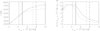 |
Fig. 11. Left panel: cuts through EOS table showing T(eint) for fixed ρ values. The solid line indicates densities corresponding to 600 km and dashed line indicates densities corresponding to 1100 km. The vertical solid and dashed thin lines indicate the values of eint corresponding to 600 and 1100 km. The vertical solid and dashed thick lines represent eint + ηAJ2, taking the same value for ηAJ2 = 107, as per Fig. 10. Right panel: same but for the gradient dT/deint. |
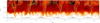 |
Fig. 12. Time series of vertical cuts showing the temperature structure (red colors), contours of log10( |

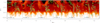 |
Fig. 13. Time series of vertical cuts showing the temperature structure (red colors), contours of log10( |

4.1. Spatial distribution of heating
In order to better understand why the average temperature increase is significantly lower in the U-AD simulations compared to the D-AD simulations, Figs. 12 and 13 show several vertical cuts of snapshots at different moments of the simulation with representative structures in both cases. Figure 12 shows the evolution of a typical vertical kG flux tube rooted in an intergranular lane and expanding with height. The structure of the flux tube can be followed by the evolution of plasma β contours (blue lines). The plasma inside these contours has β < 1 and is magnetically dominated. We note the good correlation between the locations of low plasma β regions and large heating term regions (yellow contours) in Fig. 12. The regions in which the heating term is large follow the borders of the flux tube. This is not surprising since currents are largest at these locations. Moreover, the contours of  correlate well with locations with low temperatures (dark red colors) at the tube borders. This correlation is especially evident in the upper layers of the simulation domain. The majority of these low-temperature regions are produced by longitudinal shocks and coincide with low density areas where the collisional coefficient αn entering Eq. (5) is small leading to large values of ηA. Therefore we conclude that in the U-AD simulations with smooth and unipolar fields, the contribution of temperature effects to the heating term,
  , dominates over the contribution of the effects of currents. The heating is produced essentially in areas with low temperature and has less impact on the mean temperature increase in the chromosphere.
Figure 13 gives the evolution of a typical magnetic structure in the D-AD simulation. The structure of the field is significantly different in this case and no well-formed flux tube is observed. We note that due to the generally weaker fields we do not plot the contours of log10 β = 0, but rather log10 β = 1, since the former regions are rather scarce in the photosphere. Nevertheless, it can be noticed that log10 β and log10  contours are still well correlated, i.e., the largest heating is related to areas with small β. At the same time, there is not so good correlation between the areas with large heating term and those with low temperature, as in the U-AD case. The highest heating is frequently located along the inclined canopies in the middle and upper photosphere. In the upper layers, there are still cases where low-temperature areas coincide with large
  , however it must be noted that the majority of these heating events are located in the upper photospheric regions, which agrees with Fig. 10. Therefore, since the heating is mainly produced at places that do not have significantly lower temperatures (and densities), we conclude that it is dominated by the distribution of currents rather than by temperature effects as in the U-AD case, and this makes the overall effect on the average temperature increase more efficient.
Yet another argument related to plasma ionization explains why adding the same amount of energy to the dense photospheric plasma results in larger effects on temperature, compared to the less dense chromospheric plasma. In the photosphere, the additional energy of the  term is employed essentially for increasing the temperature of the plasma. However, at chromospheric heights, the energy from
  is employed for both, increasing the plasma temperature, and ionization of the plasma. Therefore, the same amount of
  in the chromosphere results in significantly less temperature increase, compared to the photosphere. Figure 11 quantifies this argument using the EOS table employed in our code. It shows cuts through the EOS table T(eint, ρ) (left panel), and the derivative dT/deint(right panel) for fixed values of density ρ, corresponding to the typical values in the photosphere and chromosphere. Because the gradient dT/deint is about five times larger in the photosphere than in the chromosphere, the same amount of ηAJ2 leads to about five times larger temperature increase in the photosphere than in the chromosphere (720 versus 130 K in the case shown in the figure).
In order to further justify the above conclusions, Figs. 14 and 15 present correlations between the amplitudes of the flong and falf components and the heating term at a height of 1.1 Mm (for U-AD case) and at height 0.6 Mm (for D-AD case). In order to better visualize the presence or absence of correlation we computed a linear fit to the maxima of distributions for a given value of f, shown as light blue lines in the figure. This was carried out separately for the positive and negative values of f quantities. The behavior of the ffast is similar to flong, and is not shown in the figures.
There is only a weak correlation between the heating term and the falf quantity (selecting incompressible Alfvén waves) in the U-AD case, Fig. 14, right panel. The flong component (selecting compressible waves with velocities along the field) shows a correlation in a way that larger heating corresponds to larger negative values of flong. The longitudinal velocity at the studied heights has a well-developed non-linear behavior with shocks propagating along flux tubes. The negative values of flong spatially coincide with rarefactions produced by shocks, implying larger instantaneous ηA, i.e., the behavior discussed in the section above. We do not expect that this correlation changes even if non-instantaneous ionization is considered in the chromosphere, since the influence of density on the collisional parameter αn (and ηA) is significantly more pronounced than the influence of the ionization fraction, ξn. The parameter αn changes with density on an exponential scale while the ionization fraction, ξn in Eq. (5), changes on a linear scale. Therefore, we conclude that the areas with a large heating term due to the AD effect coincide with rarefactions produced by longitudinal shock waves in the unipolar U-AD simulation.
The bidimensional histograms for the D-AD case show a different behavior; see Fig. 15. The flong shows a more symmetric behavior with heating increasing with the absolute value of its amplitude. There is also a correlation for the falf quantity, showing an increase of the heating for positive values of falf (coinciding with upflows). This behavior is the opposite of the U-AD case. Locations with positive velocities do not correlate with the rarefaction sites, therefore the maximum heating is produced outside low density areas. This behavior confirms the visual impressions from Fig. 13.
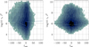 |
Fig. 14. Bidimensional histograms showing the correlation between the heating term and flong (left panel) and falf (right panel), for the U-AD runs. The color scale indicates the log10 of the number of points with a given combination of values at the axes. Inclined solid lines represent the linear fit to the distribution, done separately for positive and negative values. |
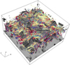 |
Fig. 16. Three-dimensional view of a simulation snapshot of the D-AD run. The grayscale image at the bottom shows the temperature at −0.5 Mm, below the surface. Colored lines are magnetic field lines; the colors indicate the vertical magnetic field strength, where blue represents negative polarity, red indicates positive polarity, and yellow represents horizontal field. The gray contours at the upper part of the domain follow regions with the heating term log10( |

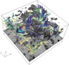 |
Fig. 17. Three-dimensional view of a simulation snapshot of the U-AD run. The grayscale image at the bottom shows temperature at −0.5 Mm, below the surface. Colored lines are magnetic field lines, the colors indicate the vertical magnetic field strength, where blue represents negative polarity, red indicates positive polarity, and yellow represents horizontal field. The gray contours at the upper part of the domain follow regions with the heating term log10( |

4.2. Three-dimensional view of the structures and heating events
Figures 16 and 17 present a three-dimensional view of the simulation domains for two selected snapshots of the D-AD and U-AD runs. The full picture of the complex interactions between the flows, magnetic field structures, and heating events can only be fully appreciated in three dimensions. The movies available online show this complexity.
The low-lying loops in the D-AD runs form a carpet of strongly inclined fields that determine the spatial structure of the locations with strong heating events. It can be appreciated in Fig. 16 that the contours with large values of  (dark gray) follow nearly horizontal fibril-like structures formed by the magnetic fields and connecting regions with opposite polarities. These fibrils are often located above areas with the strongest fields. The movies show that their typical lifetimes are on the order of minutes. No such fibrils are observed in the upper layers of the domain since the field lines essentially connect below and do not provide sufficient currents. This is also in agreement with what was previously concluded from Fig. 10. All in all, the structuring of the heating events in horizontal fibrils resembles the observed structure of the quiet solar chromosphere.
The three-dimensional evolution in both cases clearly shows that the heating due to the ambipolar diffusion effect is intimately related to the structures formed by the magnetic fields in the Sun. The presence of structuring down to small scales, together with the action of the ambipolar diffusion, causes a larger average effect on the temperature than with the presence of strong unipolar magnetic field concentrations. These initial conclusions will need further exploration in a more detailed study.
5. Discussion and conclusions
This work presents the first fully three-dimensional simulations of solar magneto-convection up to chromospheric heights including one of the most important non-ideal effects due to the presence of neutrals in the solar plasma, the ambipolar diffusion. The comparison of models obtained with exactly the same numerical setup but including/excluding the ambipolar diffusion, reveals that the latter causes appreciable effects on the dynamic and thermal structure of the chromosphere in several ways. The following paragraphs summarize our main results.
Our results show that waves, excited by convective motions in the simulations, and propagating to chromospheric heights, are significantly affected by the ambipolar diffusion. We observe height and frequency dependent variations of the wave amplitudes. The variations of the amplitudes also depend on the velocity projection related to the magnetic field vector, i.e., on the wave mode. In general, more complex and structured fields of the battery-generated dynamo D-AD run cause larger effects on the wave amplitudes.
We observe an appreciable absorption of the magnetic Poynting flux in the simulations where the ambipolar diffusion is switched on. This absorption reaches 90% in the D-AD simulations, and it is lower, reaching up to 30%, in the U-AD simulations. The absorption shows a weak frequency dependence and is appreciated at heights above 0.5 Mm where the heating term,  , is the largest.
The Poynting flux absorption profiles and the wave amplitude depression profiles generally do not coincide. While the amplitude maps give the amount of the available kinetic energy at a given height and frequency, the Poynting flux maps give information about the electromagnetic energy propagation and are fundamentally different physical quantities. There can be a different explanation for the wave amplitude variations between the AD and noAD runs, such as the change of the average structure of the magnetic field caused by the ambipolar diffusion or its influence on the mode transformation process. However, the Poynting flux decrease in the AD runs compared to the noAD runs clearly tells us that the magnetic energy of the waves has been converted into heat.
The average effect of the ambipolar diffusion on the temperature structure is more pronounced in the D-AD run compared to the U-AD run. Our analysis reveals that this is caused by the existence of fields that are highly structured on small scales in the D-AD runs producing a strong ambipolar heating over most of the photosphere already, where the plasma density is high. In the U-AD runs the strong heating only exists at chromospheric heights where the plasma density is low. At chromospheric heights, the additional energy from  term is employed not only for plasma temperature increase but also for plasma ionization, therefore its impact into the mean temperature structure is significantly less pronounced compared to the case when the same amount of energy is added in the photosphere.
In the U-AD runs, the locations of strong heating are spatially and temporally correlated with rarefactions caused by longitudinal shock waves. This causes the correlation between the amplitude of the downward longitudinal velocity and the amplitude of the heating term, ηAJ⊥. In the D-AD runs, the amplitude of the heating term is correlated with the amplitudes of the falf quantity (selecting incompressible waves). Therefore, the heating is produced mostly by variations of currents, J, rather than ηA, causing a larger average effect on the temperature increase. The locations with strong heating are very well correlated with low plasma β locations in the U-AD runs. This correlation is not so good for the D-AD runs with generally weaker fields.
The three-dimensional representation of the heating events reveals that they form fibril-like structures in the D-AD simulation, which has a carpet of horizontal fields in the upper photosphere and low chromosphere. The fibrils connect regions with fields of opposite polarities and the lifetime of such fibrils is very short, on the order of one minute. In contrast, the heating events form sheet-like structures in the U-AD simulation, following the rarefactions attached to chromospheric shocks. Their lifetimes are usually larger, on the order of several minutes.
Some of our conclusions above reveal similar features and reinforce the conclusions from previous studies of the effects of the ambipolar diffusion on chromospheric waves, current dissipation, and heating, as mentioned in the Introduction (Goodman 2000, 2011; Khomenko & Collados 2012a,b; Martínez-Sykora et al. 2012, 2016, 2017; Shelyag et al. 2016; Przybylski et al. 2018). In general, we observe the conversion of the magnetic energy into heat in terms of Poynting flux absorption and we confirm its effect on the average temperature structure of the chromosphere. Due to the simplicity of our chromospheric RT, our model does not allow us to make quantitative conclusions about the temperature increase. We can put a lower bound on the energization of the chromosphere due to AD effect. Our D-AD runs with battery-excited dynamo fields give the basal level of magnetization in the Sun. The ambipolar heating of those areas gives us a low bound to the heating in the quietest regions of the Sun. The fact that the ambipolar diffusion shows appreciable effects on the temperature structure of the atmosphere containing only this kind of weakest fields is encouraging. It confirms the potential significance of this effect for the solution of the problem of heating of the solar chromosphere.
The heating efficiency is proportional to the ambipolar diffusion coefficient, ηA, and to the current density perpendicular to the magnetic field, J⊥. The former, ηA, is a function of the ionization fraction, collisional frequency, and magnetic field strength. The dependence on the collision frequency is the strongest since it is proportional to density and changes exponentially with height in the solar atmosphere. Therefore, prior to analyzing the simulations presented in this work, we expected that the heating due to ambipolar diffusion effects would be larger in the model with stronger field structures, i.e., in the U-AD runs. Nevertheless, our analysis unexpectedly revealed the opposite. We obtain that the efficiency of the heating is more linked to the presence of currents structured at small scales than to the variations of the neutrals fraction and density (collisional frequency). Since the ambipolar diffusion is acting at small scales (see Khomenko et al. 2014b), the efficiency of the heating increases naturally when such currents are present, as happens in the D-AD run. In other words, the effects of small-scale currents are more important than the effects of the strength of the field itself or than the effects of the change of the thermodynamic structure. This means that, even if non-equilibrium ionization and more complex RT effects are included in further modeling, we do not expect that the main conclusions of our study will change.
Our simulations also reveal that the variation of the wave amplitude due to ambipolar diffusion is a sensible function of their frequency and wave mode. This result indirectly confirms the conclusions by Przybylski et al. (2018) obtained in a simpler controlled experiment. Overall our simulations reveal several effects that will need separate dedicated studies using less complicated and idealized modeling techniques, as for example the effect of ambipolar diffusion on wave transformation. The effect on the average structure of the field in the D-AD runs needs a separate dedicated study as well.
It is also interesting to note that heating locations form fibril-like structures in the D-AD run, resembling the structuring of the quiet chromosphere. The relation between the direction of chromospheric fibrils and the magnetic field was a subject of recent studies by de la Cruz Rodríguez & Socas-Navarro (2011) who revealed that they are not always aligned. Martínez-Sykora et al. (2016) confirmed such misalignment from two-dimensional simulations including the ambipolar diffusion effects. We observe a similar picture. While in the generally weaker areas with low-lying loops fibrils tend to be aligned with the fields, this is not the case where strong unipolar tubes are present. There, the heating locations follow the shock fronts and are in general not parallel to the fields. The relation between these elongated structures seen as heating events and the actual fibrils will also need a further study.
Movies
Movie of Fig. 16 Access here
Movie of Fig. 17 Access here
Acknowledgments
This work was supported by the Spanish Ministry of Science through the projects AYA2014-55078-P and AYA2014-60476-P, and by the European Research Council in the frame of the FP7 Specific Program IDEAS through the Starting Grant ERC-2011-StG 277829-SPIA. We acknowledge PRACE for awarding us access to resource MareNostrum based in Barcelona/Spain. EK acknowledges the support of the School of Mathematical Sciences at Monash University through the award of a Gordon Preston Sabbatical Fellowship.
References
- Anders, E., & Grevesse, N. 1989, Geochim. Cosmochim. Acta, 53, 197 [Google Scholar]
- Arber, T. D., Haynes, M., & Leake, J. E. 2007, ApJ, 666, 541 [NASA ADS] [CrossRef] [Google Scholar]
- Arber, T. D., Brady, C. S., & Shelyag, S. 2016, ApJ, 817, 94 [NASA ADS] [CrossRef] [Google Scholar]
- Ballester, J. L., Alexeev, I., Collados, M., et al. 2018, Space Sci. Rev., 214, A58 [NASA ADS] [CrossRef] [Google Scholar]
- Braginskii, S. I. 1965, Rev. Plasma Phys., 1, 205 [Google Scholar]
- Cally, P. S. 2006, Phil. Trans. R. Soc. London Ser. A, 364, 333 [Google Scholar]
- Cally, P. S. 2017, MNRAS, 466, 413 [NASA ADS] [CrossRef] [Google Scholar]
- Cally, P. S., & Goossens, M. 2008, Sol. Phys., 251, 251 [NASA ADS] [CrossRef] [Google Scholar]
- Cally, P. S., & Khomenko, E. 2018, ApJ, 856, 20 [NASA ADS] [CrossRef] [Google Scholar]
- de la Cruz Rodríguez, J., & Socas-Navarro, H. 2011, A&A, 527, L8 [NASA ADS] [CrossRef] [EDP Sciences] [Google Scholar]
- De Pontieu, B., & Haerendel, G. 1998, ApJ, 338, 729 [Google Scholar]
- Draine, B. T. 1986, MNRAS, 220, 133 [NASA ADS] [Google Scholar]
- Felipe, T. 2012, ApJ, 758, 96 [NASA ADS] [CrossRef] [Google Scholar]
- Felipe, T., Khomenko, E., & Collados, M. 2010, ApJ, 719, 357 [Google Scholar]
- Gingerich, O., Noyes, R. W., Kalkofen, W., & Cuny, Y. 1971, Sol. Phys., 18, 347 [NASA ADS] [CrossRef] [Google Scholar]
- González-Morales, P. A., Khomenko, E., Downes, T. P., & de Vicente, A. 2018, A&A, 615, A67 [NASA ADS] [CrossRef] [EDP Sciences] [Google Scholar]
- Goodman, M. L. 2000, ApJ, 533, 501 [NASA ADS] [CrossRef] [Google Scholar]
- Goodman, M. L. 2011, ApJ, 735, 45 [NASA ADS] [CrossRef] [Google Scholar]
- Goodman, M. L., & Kazeminezhad, F. 2010, ApJ, 708, 268 [NASA ADS] [CrossRef] [Google Scholar]
- Judge, P. 2008, ApJ, 683, L87 [NASA ADS] [CrossRef] [Google Scholar]
- Khomenko, E., & Cally, P. S. 2012, ApJ, 746, 68 [NASA ADS] [CrossRef] [Google Scholar]
- Khomenko, E., & Collados, M. 2006, ApJ, 653, 739 [Google Scholar]
- Khomenko, E., & Collados, M. 2012a, ApJ, 747, 87 [NASA ADS] [CrossRef] [Google Scholar]
- Khomenko, E., & Collados, M. 2012b, ASP Conf. Ser., 463, 281 [NASA ADS] [Google Scholar]
- Khomenko, E., Collados, M., Díaz, A., & Vitas, N. 2014a, Phys. Plasmas, 21, 092901 [NASA ADS] [CrossRef] [Google Scholar]
- Khomenko, E., Díaz, A., de Vicente, A., Collados, M., & Luna, M. 2014b, A&A, 565, A45 [NASA ADS] [CrossRef] [EDP Sciences] [Google Scholar]
- Khomenko, E., Vitas, N., Collados, M., & de Vicente, A. 2017, A&A, 604, A66 [NASA ADS] [CrossRef] [EDP Sciences] [Google Scholar]
- Kitiashvili, I. N., Kosovichev, A. G., Lele, S. K., Mansour, N. N., & Wray, A. A. 2013, ApJ, 770, 37 [NASA ADS] [CrossRef] [Google Scholar]
- Krasnoselskikh, V., Vekstein, G., Hudson, H. S., Bale, S. D., & Abbett, W. P. 2010, ApJ, 724, 1542 [NASA ADS] [CrossRef] [Google Scholar]
- Leake, J. E., & Arber, T. D. 2006, A&A, 450, 805 [NASA ADS] [CrossRef] [EDP Sciences] [Google Scholar]
- Lifschitz, A. E. 1989, Magnetohydrodynamics and Spectral Theory (Dordrecht: Kluwer Academic Publisher) [CrossRef] [Google Scholar]
- Martínez-Sykora, J., De Pontieu, B., & Hansteen, V. 2012, ApJ, 753, 161 [NASA ADS] [CrossRef] [Google Scholar]
- Martínez-Sykora, J., De Pontieu, B., Carlsson, M., & Hansteen, V. 2016, ApJ, 831, L1 [NASA ADS] [CrossRef] [Google Scholar]
- Martínez-Sykora, J., De Pontieu, B., Carlsson, M., et al. 2017, ApJ, 847, 36 [NASA ADS] [CrossRef] [Google Scholar]
- Mihalas, D. 1967, Meth. Comput. Phys., 7, 1 [Google Scholar]
- Moll, R., Cameron, R. H., & Schüssler, M. 2011, A&A, 533, A126 [NASA ADS] [CrossRef] [EDP Sciences] [Google Scholar]
- Moll, R., Cameron, R. H., & Schüssler, M. 2012, A&A, 541, A68 [NASA ADS] [CrossRef] [EDP Sciences] [Google Scholar]
- Nordlund, A. 1982, A&A, 107, 1 [NASA ADS] [Google Scholar]
- Nordlund, Å., & Stein, R. F. 2001, ApJ, 546, 576 [Google Scholar]
- Olson, G. L., & Kunasz, P. B. 1987, J. Quant. Spectr. Rad. Transf., 38, 325 [NASA ADS] [CrossRef] [Google Scholar]
- Przybylski, D., Shelyag, S., Khomenko, E., & de Vicente, A. 2018, ApJ, submitted [Google Scholar]
- Rijs, C., Moradi, H., Przybylski, D., & Cally, P. S. 2015, ApJ, 801, 27 [NASA ADS] [CrossRef] [Google Scholar]
- Rijs, C., Rajaguru, S. P., Przybylski, D., et al. 2016, ApJ, 817, 45 [NASA ADS] [CrossRef] [Google Scholar]
- Rozhansky, V. A., & Tsedin, L. D. 2001, Transport Phenomena in Partially Ionized Plasma (London and New York: Taylor& Francis) [Google Scholar]
- Shelyag, S., Mathioudakis, M., & Keenan, F. P. 2012, ApJ, 753, L22 [NASA ADS] [CrossRef] [Google Scholar]
- Shelyag, S., Cally, P. S., Reid, A., & Mathioudakis, M. 2013, ApJ, 776, L4 [NASA ADS] [CrossRef] [Google Scholar]
- Shelyag, S., Khomenko, E., de Vicente, A., & Przybylski, D. 2016, ApJ, 819, L11 [NASA ADS] [CrossRef] [Google Scholar]
- Song, P., & Vasyliūnas, V. M. 2011, J. Geophys. Res. Space Phys., 116, A09104 [Google Scholar]
- Spruit, H. C. 1974, Sol. Phys., 34, 277 [NASA ADS] [CrossRef] [Google Scholar]
- Stein, R. F., & Nordlund, Å. 2001, ApJ, 546, 585 [NASA ADS] [CrossRef] [Google Scholar]
- Steiner, O., Rezaei, R., Schaffenberger, W., & Wedemeyer-Böhm, S. 2008, ApJ, 680, L85 [NASA ADS] [CrossRef] [Google Scholar]
- Vögler, A., Shelyag, S., Schüssler, M., et al. 2005, A&A, 429, 335 [NASA ADS] [CrossRef] [EDP Sciences] [Google Scholar]
- Wedemeyer, S., & Steiner, O. 2014, PASJ, 66, S10 [NASA ADS] [CrossRef] [Google Scholar]
- Wedemeyer-Böhm, S., Scullion, E., Steiner, O., et al. 2012, Nature, 486, 505 [NASA ADS] [CrossRef] [PubMed] [Google Scholar]
All Tables
All Figures
|
Fig. 1. Left panel: time- and space-averaged modulus of the magnetic field strength as a function of height in the four simulation runs. Right panel: time- and space-averaged magnetic field inclinations with respect to the vertical direction. Orange solid: D-AD; orange dashed: D-noAD; violet solid: U-AD; violet dashed: U-noAD. The time averaging interval is 50 min. |
| In the text | |
|
Fig. 2. Vertical magnetic field at three selected heights for a snapshot of the D-AD run (upper row) and U-AD run (bottom row). The heights are indicated at the title of each panel. Notice the complex structure of fields in the D run, and the expansion of the magnetic field structures with height in both runs. Contours indicate the locations with zero vertical velocity at z = 0, highlighting the structure of granulation. The horizontal black line marks the location of cuts shown in Fig. 3 below. |
| In the text | |
|
Fig. 3. Cuts through the simulation snapshots over horizontal x and vertical z directions. The locations of the cuts are marked in Fig. 2. The color image shows the temperature. The black lines are the projections of the magnetic field lines into the x − z plane. Only the field lines with the average field strength above 5 G are drawn. Top panel: D-AD run; bottom panel: U-AD run. |
| In the text | |
|
Fig. 4. Bidimensional histogram showing the number of occurrences of a given value of plasma β as a function of height in D-AD run (left panel) and U-AD run (right panel). Darker colors mean larger probability of occurrence in logaritmic scale, indicated by the color bar. |
| In the text | |
|
Fig. 5. Top panels: power spectra of flong (left), ffast (middle) and falf (right) as a function of height and frequency for the D-AD run. For better visualization, the maps are scaled with a factor ρ0, the density of the unperturbed atmosphere. Bottom panels: ratio of D-AD to D-noAD power maps. The power is shown in log 10 units of J m−5 Hz−1. |
| In the text | |
|
Fig. 6. Amplitude spectra of the vertical component of the Poynting flux, |
| In the text | |
|
Fig. 7. Top panels: power spectra of flong (left), ffast (middle), and falf (right) as a function of height and frequency for the U-AD run. For better visualization, the maps are scaled with a factor ρ0, which is the density of the unperturbed atmosphere. Bottom panels: ratio of U-AD to U-noAD power maps. The power is shown in log 10 units of J m−5 Hz−1. |
| In the text | |
|
Fig. 8. Amplitude spectra of the vertical component of the Poynting flux, |
| In the text | |
|
Fig. 9. Bidimensional histograms showing the logarithm of the number of points with a given value of temperature at a given height. The darker colors mean larger number of points, indicated at the bar in log10 scale. Upper left panel: D-noAD run; upper right panel: D-AD run; bottom left panel: U-noAD run; bottom right panel: U-AD run. Yellow and light blue lines follow the maximum value of the distribution at each height for AD/noAD runs, correspondingly. |
| In the text | |
|
Fig. 10. Bidimensional histograms showing the logarithm of the number of points with a given value of the heating term, |
| In the text | |
|
Fig. 11. Left panel: cuts through EOS table showing T(eint) for fixed ρ values. The solid line indicates densities corresponding to 600 km and dashed line indicates densities corresponding to 1100 km. The vertical solid and dashed thin lines indicate the values of eint corresponding to 600 and 1100 km. The vertical solid and dashed thick lines represent eint + ηAJ2, taking the same value for ηAJ2 = 107, as per Fig. 10. Right panel: same but for the gradient dT/deint. |
| In the text | |
|
Fig. 12. Time series of vertical cuts showing the temperature structure (red colors), contours of log10( |
| In the text | |
|
Fig. 13. Time series of vertical cuts showing the temperature structure (red colors), contours of log10( |
| In the text | |
|
Fig. 14. Bidimensional histograms showing the correlation between the heating term and flong (left panel) and falf (right panel), for the U-AD runs. The color scale indicates the log10 of the number of points with a given combination of values at the axes. Inclined solid lines represent the linear fit to the distribution, done separately for positive and negative values. |
| In the text | |
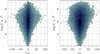 |
Fig. 15. Same as Fig. 14, but for D-AD runs. |
| In the text | |
|
Fig. 16. Three-dimensional view of a simulation snapshot of the D-AD run. The grayscale image at the bottom shows the temperature at −0.5 Mm, below the surface. Colored lines are magnetic field lines; the colors indicate the vertical magnetic field strength, where blue represents negative polarity, red indicates positive polarity, and yellow represents horizontal field. The gray contours at the upper part of the domain follow regions with the heating term log10( |
| In the text | |
|
Fig. 17. Three-dimensional view of a simulation snapshot of the U-AD run. The grayscale image at the bottom shows temperature at −0.5 Mm, below the surface. Colored lines are magnetic field lines, the colors indicate the vertical magnetic field strength, where blue represents negative polarity, red indicates positive polarity, and yellow represents horizontal field. The gray contours at the upper part of the domain follow regions with the heating term log10( |
| In the text | |
Current usage metrics show cumulative count of Article Views (full-text article views including HTML views, PDF and ePub downloads, according to the available data) and Abstracts Views on Vision4Press platform.
Data correspond to usage on the plateform after 2015. The current usage metrics is available 48-96 hours after online publication and is updated daily on week days.
Initial download of the metrics may take a while.