| Issue |
A&A
Volume 618, October 2018
|
|
|---|---|---|
| Article Number | A33 | |
| Number of page(s) | 16 | |
| Section | Planets and planetary systems | |
| DOI | https://doi.org/10.1051/0004-6361/201832867 | |
| Published online | 10 October 2018 | |
Super-Earth of 8 M⊕ in a 2.2-day orbit around the K5V star K2-216
1
Chalmers University of Technology, Department of Space, Earth and Environment, Onsala Space Observatory,
439 92
Onsala,
Sweden
e-mail: This email address is being protected from spambots. You need JavaScript enabled to view it.
2
Leiden Observatory, University of Leiden,
PO Box 9513,
2300
RA,
Leiden,
The Netherlands
3
Dipartimento di Fisica, Universitá di Torino,
via Pietro Giuria 1,
10125
Torino,
Italy
4
Department of Physics and Kavli Institute for Astrophysics and Space Research, MIT,
Cambridge,
MA
02139,
USA
5
Department of Astrophysical Sciences, Princeton University, 024B,
Peyton Hall, 4 Ivy Lane,
Princeton,
NJ
08544,
USA
6
Thüringer Landessternwarte Tautenburg,
07778
Tautenburg,
Germany
7
Department of Earth and Planetary Sciences, Tokyo Institute of Technology,
Meguro-ku,
Tokyo,
Japan
8
Rheinisches Institut für Umweltforschung an der Universität zu Köln,
Aachener Strasse 209,
50931
Köln,
Germany
9
Instituto de Astrofísica de Canarias (IAC),
38205
La Laguna,
Tenerife,
Spain
10
Departamento de Astrofísica, Universidad de La Laguna,
38206
La Laguna,
Tenerife,
Spain
11
Space Research Institute, Austrian Academy of Sciences,
Schmiedlstrasse 6,
8042
Graz,
Austria
12
Stellar Astrophysics Centre, Department of Physics and Astronomy, Aarhus University,
Ny Munkegade 120,
8000
Aarhus C,
Denmark
13
Department of Astronomy, The University of Tokyo,
7-3-1 Hongo,
Bunkyo-ku,
Tokyo
113-0033,
Japan
14
Institute of Planetary Research, German Aerospace Center (DLR),
Rutherfordstrasse 2,
12489
Berlin,
Germany
15
Department of Astronomy and McDonald Observatory, University of Texas at Austin,
2515 Speedway, Stop C1400,
Austin,
TX
78712,
USA
16
National Astronomical Observatory of Japan, NINS,
2-21-1 Osawa, Mitaka,
Tokyo
181-8588,
Japan
17
Landessternwarte Königstuhl, Zentrum für Astronomie der Universität Heidelberg,
Königstuhl 12,
69117
Heidelberg,
Germany
18
Astrobiology Center, NINS, 2-21-1 Osawa, Mitaka,
Tokyo
181-8588,
Japan
19
Center for Astronomy and Astrophysics, TU Berlin,
Hardenbergstr. 36,
10623
Berlin,
Germany
20
European Southern Observatory,
Alonso de Córdova 3107, Vitacura, Casilla,
19001
Santiago de Chile,
Chile
Received:
20
February
2018
Accepted:
28
June
2018
Abstract
Context. Although thousands of exoplanets have been discovered to date, far fewer have been fully characterised, in particular super-Earths. The KESPRINT consortium identified K2-216 as a planetary candidate host star in the K2 space mission Campaign 8 field with a transiting super-Earth. The planet has recently been validated as well.
Aims. Our aim was to confirm the detection and derive the main physical characteristics of K2-216 b, including the mass.
Methods. We performed a series of follow-up observations: high-resolution imaging with the FastCam camera at the TCS and the Infrared Camera and Spectrograph at Subaru, and high-resolution spectroscopy with HARPS (La Silla), HARPS-N (TNG), and FIES (NOT). The stellar spectra were analyzed with the SpecMatch-Emp and SME codes to derive the fundamental stellar properties. We analyzed the K2 light curve with the pyaneti software. The radial velocity measurements were modelled with both a Gaussian process (GP) regression and the so-called floating chunk offset (FCO) technique to simultaneously model the planetary signal and correlated noise associated with stellar activity.
Results. Imaging confirms that K2-216 is a single star. Our analysis discloses that the star is a moderately active K5V star of mass 0.70 ± 0.03 M⊙ and radius 0.72 ± 0.03 R⊙. Planet b is found to have a radius of 1.75−0.10+0.17 R⊕ and a 2.17-day orbit in agreement with previous results. We find consistent results for the planet mass from both models: Mp ≈ 7.4 ± 2.2 M⊕ from the GP regression and Mp ≈ 8.0 ± 1.6 M⊕ from the FCO technique, which implies that this planet is a super-Earth. The incident stellar flux is 2.48−48+220 F⊕.
Conclusions. The planet parameters put planet b in the middle of, or just below, the gap of the radius distribution of small planets. The density is consistent with a rocky composition of primarily iron and magnesium silicate. In agreement with theoretical predictions, we find that the planet is a remnant core, stripped of its atmosphere, and is one of the largest planets found that has lost its atmosphere.
Key words: planetary systems / stars: individual: K2-216 / techniques: photometric / techniques: radial velocities / planets and satellites: atmospheres / planets and satellites: composition
© ESO 2018
1 Introduction
The NASA K2 mission (Howell et al. 2014) is continuing the success of the Kepler space mission by targeting stars in the ecliptic plane through high-precision time-series photometry. Thousands of Kepler/K2 exoplanet candidates have been discovered to date and hundreds have been confirmed and characterised. One of the surprises was the vast diversity of planets, in particular planets with radii between Earth and Neptune (3.9 R⊕), with no counterparts in our solar system. Short-period super-Earth planets, Rp ≈ 1− 1.75 R⊕ (Lopez & Fortney 2014; Fulton et al. 2017) have been found to be very common based on planet occurrence rates and planet candidates discovered by Kepler (Burke et al. 2015), although the number of well-characterised super-Earths are still low. Only a few dozen have both measured radius and mass1 as of June 2018, and hence the composition and internal structure for the remaining super-Earths are unknown.
A bimodal radius distribution of small exoplanets at short orbital period was discovered by Fulton et al. (2017) using spectroscopic stellar parameters and by Van Eylen et al. (2018) using asteroseismic stellar parameters. These findings show that very few planets at P < 100 days have sizes between 1.5 and 2 R⊕. The gap is predicted by photo-evaporation models (Lopez & Fortney 2013, 2014; Owen & Wu 2013, 2017; Jin et al. 2014; Chen & Rogers 2016; Jin & Mordasini 2018), in which close-in planets (a < 0.1 AU) can lose their entire atmosphere within a few hundred Myr owing to intense stellar radiation. The mini-Neptunes and super-Earths thus appear to be two distinct classes with radii of ~ 2.5 R⊕ and ~ 1.5 R⊕, respectively.These predictions, however, need to be tested against well-characterised planets.
The work described in this paper is part of a larger programme performed by the international KESPRINT consortium2, which combine K2 photometry with ground-based follow-up observations in order to confirm and characterise exoplanetary candidates (e.g. Eigmüller et al. 2017; Guenther et al. 2017; Nowak et al. 2017; Niraula et al. 2017; Livingston et al. 2018; Hirano et al. 2018; Smith et al. 2018). When processing the K2 Campaign 8 light curves, we found a super-Earth candidate around K2-216 for which we proceeded with follow-up observations and characterisation described in this paper. During our work, planet b was recently validated by Mayo et al. (2018). In this paper, we confirm the planet and derive the previously unknown mass from radial velocity (RV) measurements.
The K2 photometry and transit detection are presented in Sect. 2. Ground-based follow-up observations (high resolution imaging and spectroscopy) are presented in Sect. 3. We analyze the star in Sect. 4 to obtain the necessary stellar mass and radius for the transit analysis performed in Sect. 5, and the RV analysis carried out in Sect. 6. We end the paper with a discussion and summary in Sects. 7 and 8, respectively.
2 K2 photometry and transit detection
Observations of the K2 Field 8 took place from January 4 to March 23, 2016. The telescope was pointed at the coordinates α = 01h05m21s and δ = +05°15′44′′ (J2000). A total of 24 187 long-cadence (29.4 min integration time) and 55 short-cadence (1 min integration time) targets were observed.
We downloaded the K2 Campaign 8 data from the Mikulski Archive for Space Telescopes3 (MAST). For the detection of transiting candidates, we searched the data using three different methods, optimised for space-based photometry: (i) the EXOTRANS (Grziwa et al. 2012) routines, (ii) the Détection Spécialisée de Transits (DST) software (Cabrera et al. 2012), and (iii) a method similar to that described by Vanderburg & Johnson (2014). The codes have been used extensively on CoRoT, Kepler and other K2 campaigns. The strategy of using different software has been shown to be successful, since both the false alarm and non-detections are model dependent.
The EXOTRANS and DST methods were applied to the pre-processed light curves by Vanderburg using the method described in Vanderburg& Johnson (2014). The EXOTRANS method is built on a combination of the wavelet-based filter technique VARLET (Grziwa & Pätzold 2016) and a modified version of the BLS (Box-fitting Least Squares; Kovács et al. 2002) algorithm to detect the most significant transit. When a significant transit is detected, the Advanced BLS removes a detected transit using a second wavelet based filter routine known as PHALET. This routine combines phase-folding and wavelet based approximation to recreate and remove periodic features in light curves. After removing a detected transit, the light curve is searched again for additional transits. This process is repeated 15 times to detect multi-planet systems. Since the detected features are completely removed, transits near resonant orbits are easily found. The DST method aims at a specialised detection of transits by improving the consideration of the transit shape and the presence of transit timing variations. The same number of free parameters as BLS are used, and the code implements better statistics with signal detection. In the third method, described in more detail by Dai et al. (2016) and Livingston et al. (2018), we extracted aperture photometry and image centroid position information from the K2 pixel-level data to decorrelate the flux variation from the rolling motion of the telescope to produce our own light curves.The transit detection routine utilises the standard BLS routine and an optimal frequency sampling (Ofir 2014).
A shallow transit signal was discovered by all three methods in the light curve of K2-216 (EPIC 220481411) with a period of ~ 2.2 days and a depth of ~0.05% consistent with a super-Earth orbiting a K5V star. We searched for even-odd transit depth variation and secondary eclipse, which would point to a binary scenario, but neither were detected within 1σ. K2-216 was proposed by programme GO8042 and observed in the long-cadence mode. The basic parameters of the star are listed in Table 1. The full pre-processed light curve by Vanderburg4 is shown in Fig. 1 in which 36 clear transits are denoted with dotted vertical lines.
Main identifiers, coordinates, optical and infrared magnitudes, parallax, and systemic velocity of K2-216.
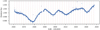 |
Fig. 1 Full pre-processed light curve of K2-216 by Vanderburg. The stellar activity is seen as the long period modulation. The narrow and shallow 36 planet transits used in the analysis are indicated with dotted vertical lines. |
3 Ground-based follow-up
Follow-up observations were performed to determine whether the signal is from a planet and to obtain further information on the planet properties. High-resolution imaging was used to check if the transit is a false positive from a fainter unresolved binary included in the K2 sky-projected pixel size of ~ 4′′ in Sects. 3.1–3.3. The presence of a binary can lead to an erroneous radius of the transiting object, which propagates into the density; this is important for distinguishing between rocky planets and those with an envelope (mini-Neptunes). The binary can be either an unrelated background system or a companion to the primary star. The planetary nature of the transit was then confirmed by our high-resolution RV measurements described in Sect. 3.4, which also allows a measure of its mass (Sect. 6). This data was also used to derive stellar fundamental parameters with spectral analysis codes (Sect. 4).
3.1 FastCam imaging and data reduction
We performed Lucky Imaging (LI) of K2-216 with the FastCam camera (Oscoz et al. 2008) at 1.55 m Telescopio Carlos Sánchez (TCS). The FastCam is a very low noise, high-speed electron-multiplying charge-coupled device (CCD) camera with 512 × 512 pixels, a physical pixel size of 16 μm, and a field of view of 21.′′2 × 21.′′2. On the night of September 6 (UT), 2016, 10 000 individual frames of K2-216 were collected in the Johnson-Cousins infrared I-band (880 nm) with an exposure time of 50 ms for each frame. The typical Strehl ratio in our observation varies with the percentage of the best-quality frames chosen in the reduction process as follows: from 0.05 for the 90% to 0.10 for 1% best images. In order to construct a high-resolution, long-exposure image, each individual frame was bias-subtracted, aligned and co-added, and then processed with the FastCam dedicated software developed at the Universidad Politécnicade Cartagena (Labadie et al. 2010; Jódar et al. 2013). The inset in Fig. 2 shows a high-resolution image, which was constructed by co-addition of the 30% best images, with a 150 s total exposure time. Figure 2 also shows the 5σ contrast curve, which quantitatively describes the detection limits of nearby possible companions that are computed based on the scatter within the annulus as a function of angular separation from the target centroid (Cortés-Contreras et al. 2017). As shown by the contrast curve, no bright companion was detectable within 8′′. Between 2′′ and 8′′ separation, we can exclude companions ≈6 × 10⁻³ times brighter than K2-216.
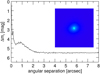 |
Fig. 2 I-band magnitude 5σ contrast curve as a function of angular separation up to 8′′ from K2-216 obtained with the FastCam camera at TCS. The inset shows the 8′′× 8′′ image. |
3.2 Subaru/IRCS AO imaging and data reduction
In order to further check for possible unresolved eclipsing binaries mimicking planetary transits, we imaged K2-216 with the Infrared Camera and Spectrograph (IRCS; Kobayashi et al. 2000) with the adaptive optics (AO) system (Hayano et al. 2010) on the Subaru 8.2 m telescope producing diffraction limited images in the 2− 5 μm range.
The high-resolution mode was selected at a pixel scale of 0.′′ 0206 per pixel, and a field of view of 21′′× 21′′. Adopting K2-216 itself as a natural guide star, we performed AO imaging on November 6, 2016 in the H-band (1630 nm) with two different exposures. The first sequence consists of a short exposure (0.4 s × 3 co-additions) with the five-point dithering to obtain unsaturated target images for the absolute flux calibration. We then repeated longer exposures (5 s ×3 co-additions) with the same five-point dithering for saturated images to look for faint nearby companions. The total scientific exposure time amounted to 225 s. We reduced the IRCS AO data following Hirano et al. (2016); we applied the dark subtraction, flat fielding, distortion correction, and aligned the frames, which were subsequently median-combined to obtain the final images for unsaturated and saturated frames, respectively.
We found that the full width at half maximum (FWHM) of K2-216 is 0.′′ 096, as measured from the combined unsaturated image. The inset of Fig. 3 shows the combined saturated image with a field of view of 4′′× 4′′. To estimate the contrast achieved by the IRCS imaging, we convolved the combined saturated image with the target’s FWHM and computed the scatter within the small annulus centred at the centroid of the target. The 5σ contrast curve as a function of angular separation from the target is drawn in Fig. 3. No bright nearby sources were found around K2-216. For instance, the contrast curve shows that at a separation of 0.′′ 5 (1.′′0), companions brighter than ΔmH ~ 5 mag (~ 7.5 mag) would have been detected with >5σ. Thus, we can exclude companions brighter than 1 × 10⁻³ of the target star at a separation of 1′′.
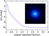 |
Fig. 3 H-band (1630 nm) 5σ magnitude contrast curve as a function of angular separation from K2-216 obtained with IRCS/Subaru. The inset shows the 4′′ × 4′′ saturated image. |
3.3 NESSI imaging
For comparison with our FastCam and IRCS imaging, we also show speckle imaging of K2-216 performed with the NASA Exoplanet Star and Speckle Imager (NESSI; Scott et al. 2016, Scott et al., in prep.) at the WIYN 3.5 m telescope in Fig. 4. The images were retrieved from ExoFop5 (with permission from the observers). The contrast curves based on the same data were also used in Mayo et al. (2018) to calculate the false-positive probabilities (FAP). The observations were conducted at 562 nm (r-narrowband) and 832 nm (z-narrowband) simultaneously on November 14, 2016. The data were collected and reduced following the procedures described by Howell et al. (2011). The resulting reconstructed images of the host star are 4.′′ 6 × 4.′′6 with a resolution close to the diffraction limit of the telescope (0.′′040 at 562 nm and 0.′′060 at 832 nm). No secondary sources were detected in the reconstructed images. We produced the 5σ detection limits from the reconstructed images using a series of concentric annuli as shown up to 1.′′ 2 in Fig. 4.
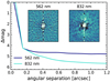 |
Fig. 4 Reconstructed images in the r- and z-narrowbands from NESSI/WIYN speckle interferometry and the resulting 5σ contrast curves. The inset images are 1.′′2 × 1.′′2. Northeast isup and to the left. |
3.4 High-resolution spectroscopy
We performed high-resolution spectroscopy to obtain RV measurements with three different instruments: FIES, HARPS, and HARPS-N. All RVs are listed in Table 2.
FIES: we started the RV follow-up of K2-216 with the FIbre-fed Échelle Spectrograph (FIES; Frandsen & Lindberg 1999; Telting et al. 2014) mounted at the 2.56 m Nordic Optical Telescope (NOT) of Roque de los Muchachos Observatory (La Palma, Spain). Eight high-resolution spectra (R ≈ 67 000) were gathered between September and November 2016, as part of our K2 follow-up programmes 53-016, 54-027, and 54-211. To account for the RV shift caused by the replacement of the CCD, which occurred on 30 September 2016, we treated the spectra taken in September 2016 and those acquired in October–November 2016 as two independent data sets. We set the exposure time to 3600 s and followed the same observing strategy described in Gandolfi et al. (2013, 2015), i.e. we traced the RV drift of the instrument by bracketing the science exposures with long-exposed ThAr spectra. The data reduction was performed using standard IRAF and IDL routines, which include bias subtraction, flat fielding, order tracing and extraction, and wavelength calibration. Radial velocities were extracted via multi-order cross-correlations using the stellar spectrum (one per CCD) with the highest signal-to-noise ratio (S/N) as a template.
HARPS and HARPS-N are fibre-fed, cross-dispersed, échelle spectrographs (R ≈ 115 000), which are designed to achieve a very high-precision and long-term RV measurements. We gathered nine spectra with the HARPS spectrograph (Mayor et al. 2003) mounted at the ESO 3.6 m telescope of La Silla observatory (Chile), between October 2016 and November2017, as part of the observing programmes 098.C-0860, 099.C-0491, and 0100.C-0808. We also collected 13 spectra with the HARPS-N spectrograph (Cosentino et al. 2012) attached at the Telescopio Nazionale Galileo (TNG) of Roque de los Muchachos Observatory (La Palma, Spain), between October 2016 and January 2018, during the observing programmes CAT16B_61, CAT17A_91, A36TAC_12, and OPT17B_59. We reduced the data using the dedicated off-line HARPS and HARPS-N pipeline and extracted the RVs via cross-correlation with a K5 numerical mask (Baranne et al. 1996; Pepe et al. 2002). The pipeline also provides the bisector inverse slope (BIS) and FWHM of the cross-correlation function (CCF), and the log  activity index of the Ca II H & K lines; these are all listed in Table 2. Since the pipelines do not derive the uncertainties for BIS and FWHM we have assumed error bars twice as large as the corresponding RV uncertainties in our analysis. The spectra haveS/N per pixel at 5500 Å in the range 20–45, except for one of the HARPS and two of the HARPS-N measurements with S/N < 20 that were not used in the RV analysis. In the sixth column, the RVs used in the Gaussian Process (GP) regression analysis (Sect. 6.1) are denoted, and in the seventh column we list the division of chunks used in the floating chunk offset (FCO) technique in Sect. 6.2.
FIES, HARPS, and HARPS-N RV measurements of K2-216.
4 Stellar analysis
The stellar mass and radius needed for the transit and RV analyses can be determined in a number of ways. In this paper we have used several different methods which requires stellar fundamental parameters as input (Teff, [Fe/H], log g⋆, ρ*, and distance).
4.1 Spectral analysis
In order to derive the stellar fundamental parameters Teff, log g⋆, and [Fe/H], we analyzed the co-added HARPS-N (S∕N = 89) and HARPS (S∕N = 94) spectra with the spectral analysis package Spectroscopy Made Easy (SME; Valenti & Piskunov 1996; Valenti & Fischer 2005; Piskunov & Valenti 2017). Utilising grids of stellar atmosphere models, based on pre-calculated 1D or 3D, local thermal equilibrium (LTE) or non-LTE models, SME calculates, for a set of given stellar parameters, synthetic spectra of stars and fits them to observed spectra using a χ2 -minimising procedure. We used the non-LTE SME version 5.2.2 and the ATLAS 12 model spectra (Kurucz 2013) to fit spectral features sensitive to different photospheric parameters. We followed the procedure in Fridlund et al. (2017). In summary, we used the profile of the line wings of the Hα and Hβ lines to determine the effective temperature, Teff (Fuhrmann et al. 1993, 1994). The line cores were excluded owing to its origin in layers above the photosphere. The stellar surface gravity, log g⋆, was estimated from the line wings of the Ca I λλ6102, 6122, 6162 triplet, and the Ca I λ6439 line. The Mg I λλ5167, 5172, 5183 triplet, which also can be used to determine log g⋆, was not used because of problems with the density of metal lines contaminating the shape of the wings of the Mg lines. The microturbulent velocity, Vmic, and the macroturbulent velocity, Vmac, were fixed to 0.5 and 1 km s−1, respectively (Doyle et al. 2014; Grassitelli et al. 2015). The projected stellar rotational velocity, V sini, and the metal abundances [Fe/H] and [Ca/H] (needed for the log g⋆ modelling) were estimated by fitting the profile of several clean and unblended metal lines between 6100 and 6500 Å. The model was also in agreement with Na doublet λλ5889 and 5896, which showed no signs of interstellar absorption. The results are listed in Table 3. We note that the spectral type of the star is at the lower end for accurate modelling with SME due to the weak line wings of the hydrogen and calcium lines, large amount of metal lines interfering with the line profiles, low S/N due to the faintness of the star, and uncertainties of model atmospheres of cool stars below ~ 4500 K.
In addition to modelling, we therefore also used the SpecMatch-Emp code (Yee et al. 2017). This code is an algorithm for characterising the properties of stars based on their optical spectra. The observed spectra are compared to a dense spectral library of 404 well-characterised stars (M5 to F1) observed by Keck/HIRES with high resolution (R ~ 55 000) and high S∕N (> 100). Since the code relies on empirical spectra, it performs particularly well for stars ~K4 and later, which are difficult to model with spectral synthesis models such as SME. However, in extreme cases, such as extremely metal poor or rich stars, the code could fail since the library includes very few such stars in each temperature bin. The SpecMatch-Emp code directly yields stellar radius rather than the surface gravity since the library stars typically have their radii calibrated using interferometry and other techniques. The direct output is thus Teff, R⋆, and [Fe/H]. We note that since the HARPS data suffers from a wavelength gap around 5320 Å because the spectrum is recorded on two separate CCD chips, the HARPS-N results should be more accurate. Following Hirano et al. (2018), prior to the analysis, we converted the co-added HARPS and HARPS-N spectra into the format of Keck/HIRES spectra that is used by SpecMatch-Emp. In doing so, we made certain that the edges of neighbouring échelle orders overlapped in wavelength. For the HARPS spectra, the gap region was replaced with a slowly varying polynomial function where each flux relative error is 100%. The validity of analysing spectroscopic data from HARPS, HARPS-N, NOT/FIES, and Subaru/HDS with SpecMatch-Emp has been tested by Hirano et al. (2018). The SpecMatch-Emp results and literature values agree with each other for Teff and stellar radii mostly within 1σ. The [Fe/H] values sometimes show a moderate disagreement, but are basically consistent within 2σ. The results are listed in Table 3 and 4.
The effective temperatures derived with SME and SpecMatch-Emp HARPS-N are in excellent agreement. The metallicities are in agreement within 1σ. Since the results are in such good agreement, and since we have no clear motivation of preferring one model over the other despite their respective possible issues, we adopted an average of the modelled effective temperatures and metallicities from SME and SpecMatch-Emp HARPS-N. Our adopted Teff is also consistent with the findings of Mayo et al. (2018; 4591 ± 50 K), whereas their metallicity (− 0.18 ± 0.08 dex) is lower than our average value, but is within 2σ. For log g⋆ we adopted the value from SpecMatch-Emp HARPS-N coupled with the Torres et al. (2010) calibration equations (see Sect. 4.2) owing to difficulties in modelling the Ca lines accurately with SME for this type of star. The log g⋆ from SpecMatch-Emp is also in perfect agreement with the adopted stellar mass and radius (Table 5) and with the results from PARAM 1.3 (Sect. 4.2). It is in addition in excellent agreement with the results from Mayo et al. (2018, log g⋆ = 4.59 ± 0.10). Within 1σ, our resulting Teff and [Fe/H] are also in agreement with the listed parameters in the Ecliptic Plane Input Catalog (EPIC; Huber et al. 2016), Teff = 4 653 ± 95 K and [Fe/H] = −0.02 ± 0.2 (dex). However, we find that the listed log g⋆ = 2.76 ± 0.43 (cgs), R⋆ = 6.9 ± 4.7 R⊙, and the stellar density of 3 × 10⁻³ g cm−3, which points to an evolved giant star at a distance of 1 159 ± 555 pc, are erroneous and in major disagreement with our spectral analysis, the Gaia distance by a factor of 10 (Sect. 4.2), and the stellar density derived by our transit modelling (Sect. 5). For the projected rotational velocity, V sini, we adopted the value determined with SME.
Using the Straizys & Kuriliene (1981) calibration scale for dwarf stars, the spectral type is defined as K5V. The adopted stellar parameters are listed in Table 5.
Spectroscopic parameters of K2-216 as derived from the co-added HARPS and HARPS-N spectra using SME and SpechMatch-emp.
Stellar mass and radius of K2-216 as derived from different methods.
Adopted stellar parameters of K2-216.
4.2 Stellar mass and radius
We calculated the stellar radius by combining the distance obtained from the Gaia DR26 parallax (8.6325 ± 0.0525 mas corresponding to a distance of 115.8 ± 0.7 pc) with our spectroscopically derived Teff and the apparent visual magnitude. We added 0.1 mas in quadrature to the parallax uncertainty to account for systematic errors of Gaia’s astrometry (Luri et al. 2018). We first calculated the luminosity from the relations MV⋆ = V − 5 × log10(d) + 5 + AV, Mbol⋆ = MV⋆ + BCv, and Mbol⋆ − Mbol,⊙ = −2.5 × log10(L⋆∕L⊙), where Mbol is the absolute bolometric magnitude, BCv is the temperature-only dependent bolometric correction of − 0.64 ± 0.02 (Cox 2000), AV is the visual extinction here assumed to be zero given the proximity of K2-216, and Mbol,⊙ = +4.74. The stellar luminosity was found to be 0.19 ± 0.01 L⊙. This value was then used to calculate thestellar radius with  , which was found to be 0.72± 0.03 R⊙ (Table 4). This value is in excellent agreement with the spectroscopic radius derived using SpecMatch-Emp (0.71 ± 0.07 R⊙), but larger than that found by Mayo et al. (2018; 0.67± 0.02 R⊙), although still within 1σ. An extinction close to zero is also supported by the absence of interstellar components in the Na I doublet at 5889 Å and by following the method outlined in Gandolfi et al. (2008). This method adopted the extinction law by Cardelli et al. (1989) and assumed RV = AV∕EB-V = 3.1. A spectral energy distribution was then fitted using synthetic colours calculated ad hoc from the BT-NEXTGEN low-resolution spectrum model (Allard et al. 2011) with the K2-216 parameters.
The stellar mass must be modelled and this is carried out with four different methods. These models also produce a stellar radius, which is, however, only used as a comparison with the radius derived above. Coupling the SpecMatch-Emp modelling with the Torres et al. (2010) calibration equations, we find a stellar mass and surface gravity of 0.70 ± 0.03 M⊙ and log g⋆ = 4.57 ± 0.09 (cgs), respectively.The Torres equations were calibrated with 95 eclipsing binaries where the masses and radii were known to better than 3%. The log g⋆ is in agreement with the PARAM 1.3 result below and with Mayo et al. (2018), but higher than obtained with SME, although still within 1σ. The corresponding stellar density is in agreement with the density found from the transit modelling in Sect. 5.
We have also used the Bayesian PARAM 1.37 (da Silva et al. 2006) online applet to obtain mass, radius, and age using the PARSEC isochrones from Bressan et al. (2012). The required input is parallax, Teff, [Fe/H], and apparent visual magnitude. The results were a stellar mass of 0.71 ± 0.02 M⊙, radius of 0.66± 0.02 R⊙, surface gravity of 4.63 ± 0.02 (cgs), and age of 5.0 ± 4.1 Gyr. The mass and radius were also estimated with the Southworth (2011) calibration equations built on the basis of 90 detached eclipsing binaries with masses up to 3 M⊙. The input parameters are the stellar density (derived from transit modelling in Sect. 5), together with the spectroscopically derived Teff and [Fe/H]. Since the derived density has large uncertainties, this is propagated to the mass ( M⊙) and radius (
 R⊙). This calibration method is thus not very useful for modelling K2-216, and is therefore not used for the mass estimate. Finally, we used the BAyesian STellar Algorithm (BASTA; Silva Aguirre et al. 2015). The BASTA model uses a Bayesian approach to isochrone grid-modelling and fits observables to a grid of BaSTi isochrones (Pietrinferni et al. 2004). We fit spectroscopic (Teff, log g⋆, [Fe/H]) and photometric (ρ⋆) constraints and find a stellar mass and radius of 0.70 ± 0.03 M⊙ and 0.65 ± 0.02 R⊙, respectively, and an age of
  Gyr.
Gyr.
All estimates of the stellar mass are in very good agreement and are listed in Table 4, along witha typical mass and radius for a K5V star for comparison. We choose to adopt a value of 0.70± 0.03 M⊙ since two of the models give this stellar mass, and the third (PARAM 1.3) only slightly higher. This mass is also in excellent agreement with Mayo et al. (2018; M⋆ = 0.70 ± 0.02 M⊙).
All adopted stellar parameters are listed in Table 5.
4.3 Stellar activity and rotation period
Before analysing the RV measurements, we need to check whether they are affected by stellar activity. Photometric variability in solar-like stars can be caused by stellar activity, such as spots and plages, on a timescale comparable to the rotationperiod of the star. The presence of active regions coupled to stellar rotation distorts the spectral line profile, inducing periodic and quasi-periodic apparent RV variation, which is commonly referred to as RV jitter.
The presence of active regions hampers our capability of detecting small planets using the RV method. This is because the expected RV wobble induced by small planets is of the same order of magnitude, or even smaller, than the activity-induced jitter. Nevertheless, if the orbital period of a planet is much smaller than the stellar rotation period, then the correlated noise due to stellar rotation can easily be distinguished from the planet-induced RV signal (Hatzes et al. 2011). An inspection of the K2 light curve shows quasi-periodic photometric variations with a typical peak-to-peak amplitude of ~ 0.4−0.5%. Given the spectral type of the star, the variability is very likely associated with the presence of spots on the photosphere of the star, combined with stellar rotation and/or its harmonics8. The light curve also shows that spots evolve with a timescale that is comparable to the duration of the K2 observations (about 80 days).
Inspecting the Ca II H & K lines in the HARPS-N spectra, we find that both lines are seen in emission as shown in Fig. 5. We measure an average Ca II chromospheric activity index,  in Table 2 of − 4.668 ± 0.059 and − 4.658 ± 0.069 from HARPS and HARPS-N, respectively, indicating that the star is moderately active.
Using the code SOAP2.09 (Dumusque et al. 2014) and adopting the stellar parameters reported in Table 5, an average peak-to-peak variation of 0.45%, the same limb-darkening coefficients (LDCs) used in the transit modelling in Sect. 5, and modelling two starspots with a size relative to the star of 0.07, we found that the expected RV jitter is ~ 4 m s−1.
The upper panel of Fig. A.1 represents the generalised Lomb-Scargle (GLS; Zechmeister & Kürster 2009) periodogram of the K2 light curve of K2-216. Prior to computing the periodogram, we removed the transit signals using the best-fitting transit model derived in Sect. 5. We also subtracted a linear fit to the K2 data to remove the flux drift often observed across many K2 stars, which is likely caused by slow changes in the spacecraft orientation and/or temperature. The remaining panels of Fig. A.1 show the GLS periodograms of the RV, BIS, FWHM, and  extracted from the FIES, HARPS, and HARPS-N data, which were first combined by subtracting the corresponding means of the data sets of each instrument (Table 2). The FAPs were determined following the bootstrap technique described in Kuerster et al. (1997).
The periodogram of the K2 light curve displays a very significant peak (FAP ≪ 1%) at 30 ± 5 days (vertical dashed blue line in Fig. A.1), which we interpreted as being the rotation period of the star (Prot). Assuming that the star is seen equator-on, this value is within the limits obtained from the stellar radius and the spectroscopically derived, projected rotational velocity V sini. We found that Prot = 2πR⋆∕V should be between 9 and 32 days, including the uncertainties on V sini and R⋆.
The dashed vertical red line in Fig. A.1 indicates the orbital frequency of the transiting planet, whereas the horizontal lines represent the 1% FAP. The periodogram of the RV measurements displays a peak at the orbital frequency of the transiting planet with a FAP of 1%, which has no counterparts in the periodograms of the activity indicators, suggesting that this signal is induced by the transiting planet. We note the presence of peaks in the periodograms of BIS and FWHM whose frequencies are close to the rotation frequency of the star.
 |
Fig. 5 Cores of the Ca II K (left panel) and H (right panel) lines are seen in emission indicating activity of K2-216. |
5 Transit modelling
We used the orbital period, mid-transit time, transit depth, and transit duration identified by EXOTRANS as input values for more detailed transit modelling with the publically available software pyaneti10 (Barragán et al. 2017), which is also used in, for example, Barragán et al. (2016), Gandolfi et al. (2017), and Fridlund et al. (2017). Pyaneti is a PYTHON/FORTRAN software that infers planet parameters using Markov chain Monte Carlo (MCMC) methods based on Bayesian analysis.
The Pyaneti software allows a joint modelling of the transit and RV data. Stellar activity can, however, only be modelled in pyaneti as a coherent signal, not changing in time or phase, which is only possible when the RV observational season is small compared to the evolution timescale of active regions (e.g. Barragán et al. 2018). Since this is not the case for K2-216 where the observations extend over 440 days, we only used pyaneti to model the transit data.
In orderto prepare the light curve for pyaneti and reduce the amplitude of any long-term systematic or instrumental flux variations, we used the exotrending (Barragán & Gandolfi 2017) code to detrend the Vanderburg transit light curve (Fig. 1) by fitting a second-order polynomial to the out-of-transit data. Input to the code is the mid-time of first transit, T0, and orbital period, Porb. Three hoursaround each of the 36 transits was masked to ensure that no in-transit data were used in the detrending process.
We followed the procedure in Barragán et al. (2016) for the pyaneti transit modelling. For the mid-time of first transit (T0), the orbital period, Porb, the scaled orbital distance (a∕R⋆), the planet-to-star radius ratio (Rp /R⋆), and the impact param- eter (b ≡ acos(i)∕R⋆), we set uniform priors meaning that we adopted rectangular distributions over given ranges of the param- eter spaces. The value T0 is measured relatively precise com- pared to the cadence of the light curve, and P is measured very precise because of the large number of transits (36), and the absence of measurable transit timing variations. The ranges are thus T0 = [7394.03887, 7394.05887] (BJDTDB – 2 450 000) days, P = [2.17249, 2.17649] days, a∕R⋆ = [1.1, 50], b = [0, 1], and Rp /R⋆ = [0, 0.1]. Circular orbit was assumed, hence the eccentricity (e) was fixed to zero, and the argument of periastron, ω, was set to 90°. The transit models were integrated over ten steps to account for the long integration time (29.4 min) of K2 (Kipping 2010). We adopted the quadratic limb darkening equation by Mandel & Agol (2002), which uses the linear and quadratic coefficients u1 and u2, respectively. We followed the parametrisation  and
and  from Kipping (2013). We first ran a fit using uniform priors for the LDCs and noticed that the LDCs were not well constrained by the light curve. This is because the LDCs are not well constrained for small planets using uniform priors (e.g. Csizmadia et al. 2013). Thus, we used the online applet11 written by Eastman et al. (2013) to interpolate the Claret & Bloemen (2011) limb darkening tables to the spectroscopic parameters of K2-216 to estimate u1 and u2. These values were used to set Gaussian priors to q1 and q2 LDCs with 0.1 error bars. The planetary and orbital parameters were consistent for both LDC prior selections. We used the model with Gaussian priors on LDC for the final parameter estimation.
We explored the parameter space with 500 independent chains created randomly inside the prior ranges. We checked for convergence each 5000 iterations. Once convergence was found, we used the last 5000 iterations with a thin factor of 10 to create the posterior distributions for the fitted parameters. This led to a posterior distribution of 250 000 independent points for each parameter. The posterior distributions for all parameters were smooth and unimodal. The final planet parameters are listed in Table 6, and the resulting stellar density is listed in Table 5. The folded light curve and best-fitted model (binned to the K2 integration time to allow comparison with the data) is shown in Fig. 6.
Final K2-216 b parameters.
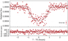 |
Fig. 6 Transit light curve folded to the orbital period of K2-216 and residuals. The red points indicate the K2 photometric data. The solid line indicates the pyaneti best-fitting transit model. |
6 Radial velocity modelling
6.1 Gaussian process regression
We used a GP regression model described by Dai et al. (2017) to simultaneously model the planetary signal and correlated noise associated with stellar activity. This code is able to fit a non-coherent signal, assuming that activity acts as a signal whose period is given by the rotation period of the star, and whose amplitude and phase change on a time scale given by the spot evolution timescale. Gaussian process describes a stochastic process as a covariance matrix whose elements are generated by user-specified kernel functions. With suitable choice of the kernel functions and the hyperparameters that specify these functions, GP can be used to model a wide range of stochastic processes. GP regression has been successfully applied to the RV analysis of several exoplanetary systems where correlated stellar noises cannot be ignored, for example, CoRoT-7 (Haywood et al. 2014), Kepler-78 (Grunblatt et al. 2015), and Kepler-21 (López-Morales et al. 2016).
Magnetic active regions on the host star, coupled with stellar rotation, result in quasi-periodic variations in both the measured RV and flux variation. Given their similar physical origin, both the quasi-periodic flux variation and correlated stellar noise in the RV measurements encode physical information about the host stars, for example the stellar rotation period and lifetime of starspots. This information is reflected in the hyperparameters of GP used to model these effects. In particular, there is a good correspondence between the stellar rotation period and the period of the covariance, T, while the correlation timescale, τ, and weighting parameter, Γ, together determine the lifetime of starspots. We can thus model both the rotational modulation in the light curve and the correlated noise in RV as GPs.
Since the K2 light curve was measured with a high-precision, high temporal sampling, and an almost continuous temporal coverage, wetrained our GP model on the K2 light curve after removal of the transits. The constraints on the hyperparameters were then used as priors in the subsequent RV analysis. We used the covariance matrix and the likelihood function described by Dai et al. (2017) and adopted a quasi-periodic kernel,
![Mathematical equation: \begin{equation*}C_{i,j} = h^2 \exp{\left[-\frac{(t_i-t_j)^2}{2\tau^2}-{\mathrm{\Gamma}} \sin^2{\frac{\pi(t_i-t_j)}{T}}\right]}+\left[\sigma_i^2+\sigma_{\text{jit}}(t_i)^2\right]\delta_{i,j} ,\end{equation*}](/articles/aa/full_html/2018/10/aa32867-18/aa32867-18-eq12.png) (1)
(1)
where Ci,j is an element of the covariance matrix, and δi,j is the Kronecker delta function. The hyperparameters of the kernel are the covariance amplitude h, T, τ, the time of ith observation, ti, and Γ which quantifies the relative importance between the squared exponential and periodic parts of the kernel. For the planetary signal, we assumed a circular Keplerian orbit. The corresponding parameters are the RV semi-amplitude, K, the orbital period, Porb, and the time of conjunction, tc. Since our data set consists of observations from several observatories, we included a separate jitter parameter, σjit, to account for additional stellar/instrumental noise, and a systematic offset, γ, for each of the instruments (Table 2). The orbital period and time of conjunction are much better measured using the transit light curve. We thus imposed Gaussian priors on Porb and tc as derived from the K2 transit modelling. We imposed a prior on T using the stellar rotation period measured from the periodogram (30 ± 5 days). The scale parameters h, τ, K, and the jitters were sampled uniformly in log space, basically imposing a Jeffrey’s priors. Uniform priors were imposed on the systematic offsets.
The likelihood function has the following form:
 (2)
(2)
where  is the likelihood, N is the number of data points, C is the covariance matrix, and r is the residual vector (the observed value minus the model value). The model includes the RV variation induced by the planet and a constant offset for each instrument.
We first located the maximum likelihood solution using the Nelder–Mead algorithm implemented in the Python package scipy. We sampled the posterior distribution using the affine-invariant MCMC implemented in the code emcee (Foreman-Mackey et al. 2013). We started 100 walkers near the maximum likelihood solution. We stopped after running the walkers for 5000 links. We checked for convergence by calculating the Gelman–Rubin statistics, which dropped below 1.03 indicating adequate convergence. We report the various parameters using the median and 16–84% percentiles of the posterior distribution. The hyperparameters were constrained to be τ =  days, Γ = 1.28 ± 0.63, and T = 28 ± 4 days. These were incorporated as priors in the subsequent GP analysis of the RV data.
We followed a similar procedure when analysing the RV data set. We first found the maximum likelihood solution and then sampled the posterior distribution with MCMC. We removed four isolated RV measurements, which were separated by more than approximately two τ from any neighbouring data points, from the GP modelling. Without neighbouring data points, the stellar variability component of these isolated data points are causally disconnected. As a result, GP tends to overfit these data points and thus underestimate the planetary signal. The removed RVs are listed in column six of Table 2. The RV semi-amplitude for planet K2-216 b was constrained to  m s−1. Using the stellar mass derived in Sect. 4.2 of 0.70 ± 0.03 M⊙, this translates to a planet mass of 7.4 ± 2.2 M⊕ with a precision in mass of 30%. The amplitude of the correlated stellar noise is hrv =
  m s−1, which agrees with the SOAP2.0 modelling in Sect. 4.3. The 95% upper bounds of the jitters were found to be < 5.1 m s−1 (FIES), < 4.7 m s−1 (FIES2), < 2.5 m s−1 (HARPS), and < 2.6 m s−1 (HARPS-N). As a comparison, keeping all the RVs with S∕N > 20, we obtain K =
  m s−1 corresponding to a planet mass of
  M⊕, and hrv =
  m s−1. Figure 7 shows the measured RV variation of K2-216 and the GP model. The folded RV diagram as a function of orbital phase is shown Fig. 8. The results are listed in Table 6.
 |
Fig. 7 Measured RV variation of K2-216 from HARPS-N (green stars), HARPS (purple diamonds), FIES (yellow circles), and FIES2 (blue triangles). The black solid line is the best fit from the GP regression model of the correlated stellar noise and the signal from K2-216 b. The signal from planet b is shown by the yellow dashed line, and the GP regression model of correlated stellar noise by the red dotted line. The lower panel shows residuals of the fit. |
 |
Fig. 8 Radial velocity curve of K2-216 phase folded to the orbital period of the planet using the GP regression model. The data are plotted with the same colour code as in Fig. 7. The resulting
K amplitude is |

6.2 Floating chunk offset technique
It is difficult to remove the influence of activity from RV measurements in a reliable way, particularly for sparse data. The GP method often gives good results, but in our case it is trained using the K2 light curve that was taken before the RV measurements. Possibly at that time the activity signal could have shown different characteristics. It is therefore important to use independent techniques, when possible, to determine the K amplitude of the orbit.
The FCO technique is another method for filtering out the effects of activity, but in a model independent way (Hatzes 2014). Basically, it fits a Keplerian orbit to RV data that have been divided into small time chunks, keeping the period fixed, but allowing the zero point offsets to float. The only assumption of the method is that the orbital period of the planet is less than the rotational period of the star or other planets. The RV variations in one time chunk is predominantly due to the orbital motion of the planet and all other variations constant. This method also naturally accounts fordifferent velocity offsets between different instruments or night-to-night systematic errors. As long as the timescales for these are shorter than the orbital period, their effects are absorbed in the calculation of the offset.
The FCO method is usually applied to ultra-short period planets (Porb < 1 day), where the orbital motion in one night can be significant (see Hatzes 2014). However, it can also be applied for planets on longer period orbits as long as these are shorter than say, the rotational period of the star. One also should have relatively high cadence measurements. In the case of K2-216, the orbital period of the planet is 2.17 days and the best estimate of the rotational period of the star is ≈ 30 days. Furthermore, we have high cadence measurement where observations were taken on several consecutive nights. The conditions are right for applying the FCO method.
The data were divided into six data sets or chunks. It is important to exclude isolated measurements, separated by more than several orbital periods, as these do not provide any shape information for the RV curve. We divided the RV data into six time chunks that were separated by no more than two days with the exception of chunk one and four, which covered time spans of three and four days, respectively. In particular, the HARPS data were divided into two chunks of which the last had only two RV measurements. In order to include these data points, but to have more shape information, the last RV value for chunk three was repeated in chunk four (and thus the time span for chunk four increased to five days). The seventh column in Table 2 shows the division of the RV chunks.
We firstchecked if the planet signal was present in our data using the so-called FCO periodogram (Hatzes 2014). For this, the RV chunks are fit using a different trial period. The resulting χ2 as a function of period is a form of a periodogram, and the χ2 should be minimised for the period that is present in the data. This was carried out with trial periods spanning 0.5–10 days. The reduced χ2 was minimised for a period of 2.17 days as shown in Fig. A.2. This confirms that the RV variations due to the planet are clearly seen in our data.
An orbital fit was then made to the chunk data using the program Gaussfit (Jefferys et al. 1988). The period and ephemeris were fixed to the transit values, but the zero point offsets for each chunk and the K amplitude were allowed to vary. The resulting K amplitude is 5.0 ± 1.0 m s−1, which corresponds to a planet mass of 8.0 ± 1.6 M⊕ (Table 6). The precision in mass is 20%. If we remove the double point in chunk four, we get essentially the same amplitude (K = 5.1 ± 1.0 m s−1). Figure 9 shows the phased orbit fit after applying the calculated offsets. Different symbols indicate the different chunks. This velocity amplitude is in very good agreement with the GP analysis. The very small differences merely reflect the variations due to a different treatment of the activity signal.
When using the FCO method, it is important to check that it can reliably recover an input K amplitude. The time sampling of the data or harmonics of the rotational period (e.g. Prot ∕2 ≈ 15 days) may effect the recovered K amplitude in a systematic way. This was explored through simulations. We first tried to account for any activity signal in a way independent of the GP model. To do this, we placed all the data on the same zero-point scale to account for the large relative offset between the HARPS and FIES data and then removed the planet signal. A Fourier analysis showed no significant peaks in the amplitude spectrum, but a weak one at 15 days with an amplitude of 3.5 m s−1. Assuming this could be the first harmonic of the rotational period we fit a sine wave to the data using this period and amplitude and took this as our activity signal. We note that a 15-day activity signal should have a much larger effect on the results of the FCO method. We then added the orbital signal of the planet to this activity signal using a range of K-amplitudes. The median error of our RV measurements is 2.8 m s−1, so we added random noise with σ =3 m s−1. We also added a large velocity offset (≈ −26 km s−1) between the simulated FIES and HARPS/N measurements. Finally, for good measure we added an additional random velocity component ranging between − 10 and + 8 m s−1 to the individual chunks to account for any additional activity jitter. For each input K-amplitude, a total of 50 sample data sets were generated using different random noise generated with different seed values. The mean and standard deviations were calculated for each. The K-amplitude was reliably recovered in the full amplitude range 1–6 m s−1. Figure A.3 shows the output K amplitude as a function of input K amplitude. The red square is the value for K2-216.
 |
Fig. 9 Radial velocity curve phase folded to the orbital period of the planet (2.17 days) using the FCO technique. The RV data from the different chunks from each spectrometer are indicated in a variety of colours and symbols. The double point used in both chunk three and four is plotted twice with a slight phase offset for clarity. Seven of the time isolated RVs have been removed from the fit. The resulting K amplitude is 5.0 ± 1.0 m s−1. The lower panel shows residuals of the fit. |
7 Discussion
Combining our mass and radius estimates of K2-216 b, we find mean densities of  g cm−3 and
  g cm−3 from the GP and FCO methods, respectively, in excellent agreement with each other. In Fig. 10, we show the position of planet b on a mass-radius diagram (FCO mass) compared to all small exoplanets (Rp ≤ 2 R⊕) with masses ≤ 30 M⊕ known to better than 20%, as listed in the NASA Exoplanet Archive. The insolation flux of the planets is colour coded. The figure also displays the Zeng et al. (2016) theoretical models of planet composition in different colours from 100% water to 100% iron. The density of K2-216 b is consistent with a rocky composition of primarily iron and magnesium silicate.
The radius of K2-216 b puts it in the middle, or just below the lower edge, of the bimodal radius distribution of small planets (Fulton et al. 2017), using the location and shape of the radius gap as estimated by Van Eylen et al. (2018) with
 (3)
(3)
where  and
and  . For a period of 2.17 days, the location of the centre of the valley is around 2.2 R⊕. This suggests that K2-216 b is a remnant core, stripped of its atmosphere.
To estimate the likelihood of K2-216 b having an extended atmosphere, we begin by considering that during the early phases of planet evolution, when a planet comes out of the proto-planetary nebula, it goes through a phase of extreme thermal Jeans escape, the so-called boil-off (Owen & Wu 2017). After this phase, the planet arrives at a more stable configuration in which the escape is driven by the stellar extreme-ultraviolet (XUV) flux (Fossati et al. 2017a). Whether a planet lies in the boil-off regime or not, can be determined on the basis of the restricted Jeans escape parameter, Λ, which is defined as (Fossati et al. 2017a)
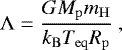 (4)
(4)
where G is the gravitational constant, mH is the hydrogen mass, kB is the Boltzmann constant, and Teq is the equilibrium temperature of the planet. When Λ ≤ 20−40, depending on the system parameters, a planet with a hydrogen-dominated atmosphere will lie in the boil-off regime (Fossati et al. 2017a). Considering the two derived planetary masses for K2-216 b, Λ ranges between 29 and 31. Assuming that the planet originally accreted a hydrogen-dominated atmosphere, following the boil-off phase, the planet will have a Λ value of about 20 (to be conservative). This value corresponds to a planetary radius of ≈ 2.6 R⊕. The right panel in Fig. 4 of Rogers et al. (2011) indicates that, following the boil-off phase K2-216 b had a hydrogen-dominated atmosphere with a mass of ≈0.1% planetary mass.
To examine whether this atmosphere would have escaped within the age of the system under the action of the high-energy (X-ray and EUV; XUV) stellar irradiation, we computed upper atmosphere models with the derived planet parameters employing the hydrodynamic code described by Kubyshkina et al. (2018). We estimated the stellar XUV flux starting from the  value derived from the spectra. We converted the measured
  value into Ca II H & K line core emission flux at 1 AU employing the equations listed in Fossati et al. (2017b), obtaining 18 erg cm−2 s−1. From this value and using the relations given by Linsky et al. (2013, 2014), we obtained a stellar Ly α flux at 1 AU of 20 erg cm−2 s−1 and an XUV flux at the planetary orbit of approximately 19 000 erg cm−2 s−1. Inserting this value and the planet parameters in the upper atmosphere code leads to mass-loss rates of 6− 9× 10⁻¹² M⊕ yr−1. This impliesthat the planet must have lost between 0.07 and 0.13% of its mass in one Gyr. Our estimated age of the system in Sect. 4.2 has very large uncertainties, but during a 5 Gyr main-sequence lifetime of the host star the planet would have lost between 0.35% and 0.65% of its mass, which is significantly larger than the predicted initial hydrogen-dominated envelope mass of 0.1%. In addition, the above mass-loss predictions should be considered to be lower limits, since the young star was significantly more active than taken into account above. Thus, even considering the large uncertainties in age, we conclude that K2-216 b likely has completely lost its primordial, hydrogen-dominated atmosphere, and is one of the largest planets found to have lost its atmosphere (see Fig. 7 in Van Eylen et al. 2018).
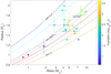 |
Fig. 10 Mass-radius diagram of all small exoplanets (Rp ≤ 2 R⊕ and Mp ≤ 30 M⊕) with a measured mass and radius to a precision better than 20% as listed in the NASA Exoplanet Archive. The colours of the planets indicate the insolation in units of log 10 (F⊕). Earth and Venus are plotted in red filled circles for comparison. The solid lines are theoretical mass-radius curves (Zeng et al. 2016); from top to bottom: 100% H2O (blue solid line), a mixture of 50% H2O and 50% MgSiO3 (cyan dashed line), 100% MgSiO3 (green solid line), a mixture of 75% MgSiO3 and 25% Fe (magenta dashed line), a mixture of 50% MgSiO3 and 50% Fe (brown solid line), a mixture of 25% MgSiO3 and 75% Fe(red dashed line), and 100% Fe (orange solid line). |
8 Summary
In this paper, we confirm the discovery of the super-Earth K2-216 b (EPIC 220481411 b) in a 2.17-day orbit transiting a moderately active K5V star at a distance of 115.8 ± 1.5 pc. We derive the mass of planet b using two different methods: first, a GP regression based on both the RV and photometric time series, and second, the FCO technique, based on RV measurements observed close in time with the assumption that the orbital period of the planet is much less than the rotational period of the star. The results are in very good agreement with each other: Mp ≈ 7.4 ± 2.2 M⊕ from the GP regression and Mp ≈ 8.0 ± 1.6 M⊕ from the FCO technique. The density is consistent with a rocky composition of primarily iron and magnesium silicate, although the uncertainties allow a range of planetary compositions. With a size of  R⊕, this planet falls within, or just below, the gap of the bimodal radius distribution where few planets are found. Our results indicate that the planet has completely lost its primordial hydrogen-dominated atmosphere, supporting the formation scenario of short-period super-Earths as remnants from mini-Neptune planets.
Acknowledgements
We thank the NOT, TNG, ESO, Subaru, and TCS staff members for their support during the observations. Based on observations obtained with (a) the Nordic Optical Telescope (NOT), operated on the island of La Palma jointly by Denmark, Finland, Iceland, Norway, and Sweden, in the Spanish Observatorio del Roque de los Muchachos (ORM) of the Instituto de Astrodísica de Canarias (IAC) (programmes 53-016, 54-027, and 54-211); (b) with the Italian Telescopio Nazionale Galileo (TNG) operated at the ORM (IAC) on the island of La Palma by the INAF Fundación Galileo Galilei (programmes CAT16B_61, CAT17A_91, A36TAC_12, and OPT17B_59); (c) the 3.6 m ESO telescope at La Silla Observatory (programmes 098.C-0860, 099.C-0491 and 0100.C-0808); (d) the Telescopio Carlos Sánchez (TCS) installed at IAC’s Observatorio del Teide, Tenerife; (e) the Subaru Telescope, operated by the National Astronomical Observatory of Japan; (f) NESSI, funded by the NASA Exoplanet Exploration Program and the NASA Ames Research Center. NESSI was built at the Ames Research Center by Steve B. Howell, Nic Scott, Elliott P. Horch, and Emmett Quigley; (g) the K2/Kepler mission. Funding for the K2/Kepler mission is provided by the NASA Science Mission Directorate. The K2 data presented in this paper were downloaded from the Mikulski Archive for Space Telescopes (MAST). STScI is operated by the Association of Universities for Research in Astronomy, Inc., under NASA contract NAS5-26555. Support for MAST for non-HST data is provided by the NASA Office of Space Science via grant NNX13AC07G and by other grants and contracts. This work has made use of SME package, which benefits from the continuing development work by J. Valenti and N. Piskunov and we gratefully acknowledge their continued support. This work has made use of the VALD database, operated at Uppsala University, the Institute of Astronomy RAS in Moscow, and the University of Vienna (Kupka et al. 2000; Ryabchikova et al. 2015). C.M.P. and M.F. gratefully acknowledge the support of the Swedish National Space Board. D.G. gratefully acknowledges the financial support of the Programma Giovani Ricercatori – Rita Levi Montalcini – Rientro dei Cervelli (2012) awarded by the Italian Ministry of Education, Universities and Research (MIUR). D.K. and L.F. acknowledge the Austrian Forschungs-förderungsgesellschaft FFG project “TAPAS4CHEOPS” P853993. Sz.C, A.P.H., M.P., and H.R. acknowledge the support of the DFG priority programme SPP 1992 “Exploring the Diversity of Extrasolar Planets” (HA 3279/12-1, PA525/18-1, PA525/19-1, PA525/20-1, and RA 714/14-1). Funding for the Stellar Astrophysics Centre is provided by the Danish National Research Foundation (grant agreement No. DNRF106). This project has received funding from the European Union’s Horizon 2020 research and innovation programme under grant agreement No. 730890. This material reflects only the authors views and the Commission is not liable for any use that may be made of the information contained therein. We thank the anonymous referee whose constructive comments led to an improvement of the paper.
Appendix A Additional figures
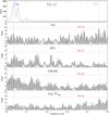 |
Fig. A.1 From top to bottom panels: generalised Lomb–Scargle periodograms of the K2 light curve, the RV measurements, BIS, FWFM of the correlation function, and the activity index |

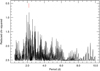 |
Fig. A.2 Floating chunk offset-periodogram over the range 0.5−10 days (χ2 vs. period). The y-axis is flipped so that a minimum appears as a peak, much like a standard periodogram. The best fit is at the planet period of 2.17 days. |
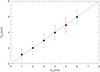 |
Fig. A.3 Output K amplitude as a function of input K amplitude using the FCO technique. |
References
- Allard, F., Homeier, D., & Freytag, B. 2011, in 16th Cambridge Workshop on Cool Stars, Stellar Systems, and the Sun, eds. C. Johns-Krull, M. K. Browning, & A. A. West, ASP Conf. Ser. 448, 91 [NASA ADS] [Google Scholar]
- Baranne, A., Queloz, D., Mayor, M., et al. 1996, A&AS, 119, 373 [NASA ADS] [CrossRef] [EDP Sciences] [Google Scholar]
- Barragán, O., & Gandolfi, D. 2017, Astrophysics Source Code Library [record ascl:1706.001] [Google Scholar]
- Barragán, O., Grziwa, S., Gandolfi, D., et al. 2016, AJ, 152, 193 [NASA ADS] [CrossRef] [Google Scholar]
- Barragán, O., Gandolfi, D., & Antoniciello, G. 2017, Astrophysics Source Code Library [record ascl:1707.003] [Google Scholar]
- Barragán, O., Gandolfi, D., Dai, F., et al. 2018, A&A, 612, A95 [NASA ADS] [CrossRef] [EDP Sciences] [Google Scholar]
- Bressan, A., Marigo, P., Girardi, L., et al. 2012, MNRAS, 427, 127 [NASA ADS] [CrossRef] [Google Scholar]
- Burke, C. J., Christiansen, J. L., Mullally, F., et al. 2015, ApJ, 809, 8 [NASA ADS] [CrossRef] [Google Scholar]
- Cabrera, J., Csizmadia, S., Erikson, A., Rauer, H., & Kirste, S. 2012, A&A, 548, A44 [NASA ADS] [CrossRef] [EDP Sciences] [Google Scholar]
- Cardelli, J. A., Clayton, G. C., & Mathis, J. S. 1989, ApJ, 345, 245 [NASA ADS] [CrossRef] [Google Scholar]
- Chen, H., & Rogers, L. A. 2016, ApJ, 831, 180 [NASA ADS] [CrossRef] [Google Scholar]
- Claret, A., & Bloemen, S. 2011, A&A, 529, A75 [NASA ADS] [CrossRef] [EDP Sciences] [Google Scholar]
- Cortés-Contreras, M., Béjar, V. J. S., Caballero, J. A., et al. 2017, A&A, 597, A47 [NASA ADS] [CrossRef] [EDP Sciences] [Google Scholar]
- Cosentino, R., Lovis, C., Pepe, F., et al. 2012, in Ground-based and Airborne Instrumentation for Astronomy IV, Proc. SPIE, 8446, 84461V [Google Scholar]
- Cox, A. N. 2000, Allen’s Astrophysical Quantities (New York: Springer) [Google Scholar]
- Csizmadia, S., Pasternacki, T., Dreyer, C., et al. 2013, A&A, 549, A9 [NASA ADS] [CrossRef] [EDP Sciences] [Google Scholar]
- Dai, F., Winn, J. N., Albrecht, S., et al. 2016, ApJ, 823, 115 [NASA ADS] [CrossRef] [Google Scholar]
- Dai, F., Winn, J. N., Gandolfi, D., et al. 2017, AJ, 154, 226 [NASA ADS] [CrossRef] [Google Scholar]
- da Silva, L., Girardi, L., Pasquini, L., et al. 2006, A&A, 458, 609 [NASA ADS] [CrossRef] [EDP Sciences] [Google Scholar]
- Doyle, A. P., Davies, G. R., Smalley, B., Chaplin, W. J., & Elsworth, Y. 2014, MNRAS, 444, 3592 [NASA ADS] [CrossRef] [Google Scholar]
- Dumusque, X., Boisse, I., & Santos, N. C. 2014, ApJ, 796, 132 [NASA ADS] [CrossRef] [Google Scholar]
- Eastman, J., Gaudi, B. S., & Agol, E. 2013, PASP, 125, 83 [NASA ADS] [CrossRef] [Google Scholar]
- Eigmüller, P., Gandolfi, D., Persson, C. M., et al. 2017, AJ, 153, 130 [NASA ADS] [CrossRef] [Google Scholar]
- Foreman-Mackey, D., Hogg, D. W., Lang, D., & Goodman, J. 2013, PASP, 125, 306 [CrossRef] [Google Scholar]
- Fossati, L., Erkaev, N. V., Lammer, H., et al. 2017a, A&A, 598, A90 [NASA ADS] [CrossRef] [EDP Sciences] [Google Scholar]
- Fossati, L., Marcelja, S. E., Staab, D., et al. 2017b, A&A, 601, A104 [NASA ADS] [CrossRef] [EDP Sciences] [Google Scholar]
- Frandsen, S., & Lindberg, B. 1999, in Astrophysics with the NOT, eds. H. Karttunen, & V. Piirola, 71 [Google Scholar]
- Fridlund, M., Gaidos, E., Barragán, O., et al. 2017, A&A, 604, A16 [NASA ADS] [CrossRef] [EDP Sciences] [Google Scholar]
- Fuhrmann, K., Axer, M., & Gehren, T. 1993, A&A, 271, 451 [NASA ADS] [Google Scholar]
- Fuhrmann, K., Axer, M., & Gehren, T. 1994, A&A, 285, 585 [NASA ADS] [Google Scholar]
- Fulton, B. J., Petigura, E. A., Howard, A. W., et al. 2017, AJ, 154, 109 [NASA ADS] [CrossRef] [Google Scholar]
- Gandolfi, D., Alcalá, J. M., Leccia, S., et al. 2008, ApJ, 687, 1303 [NASA ADS] [CrossRef] [Google Scholar]
- Gandolfi, D., Parviainen, H., Fridlund, M., et al. 2013, A&A, 557, A74 [NASA ADS] [CrossRef] [EDP Sciences] [Google Scholar]
- Gandolfi, D., Parviainen, H., Deeg, H. J., et al. 2015, A&A, 576, A11 [NASA ADS] [CrossRef] [EDP Sciences] [Google Scholar]
- Gandolfi, D., Barragán, O., Hatzes, A. P., et al. 2017, AJ, 154, 123 [NASA ADS] [CrossRef] [Google Scholar]
- Grassitelli, L., Fossati, L., Langer, N., et al. 2015, A&A, 584, L2 [NASA ADS] [CrossRef] [EDP Sciences] [Google Scholar]
- Grunblatt, S. K., Howard, A. W., & Haywood, R. D. 2015, ApJ, 808, 127 [NASA ADS] [CrossRef] [Google Scholar]
- Grziwa, S., & Pätzold, M. 2016, ArXiv e-prints [arXiv:1607.08417] [Google Scholar]
- Grziwa, S., Pätzold, M., & Carone, L. 2012, MNRAS, 420, 1045 [NASA ADS] [CrossRef] [Google Scholar]
- Guenther, E. W., Barragán, O., Dai, F., et al. 2017, A&A, 608, A93 [NASA ADS] [CrossRef] [EDP Sciences] [Google Scholar]
- Hatzes, A. P. 2014, A&A, 568, A84 [NASA ADS] [CrossRef] [EDP Sciences] [Google Scholar]
- Hatzes, A. P., Fridlund, M., Nachmani, G., et al. 2011, ApJ, 743, 75 [NASA ADS] [CrossRef] [Google Scholar]
- Hayano, Y., Takami, H., Oya, S., et al. 2010, in Adaptive Optics Systems II, Proc. SPIE, 7736, 77360N [CrossRef] [Google Scholar]
- Haywood, R. D., Collier Cameron, A., Queloz, D., et al. 2014, MNRAS, 443, 2517 [NASA ADS] [CrossRef] [Google Scholar]
- Hirano, T., Fukui, A., Mann, A. W., et al. 2016, ApJ, 820, 41 [NASA ADS] [CrossRef] [Google Scholar]
- Hirano, T., Dai, F., Gandolfi, D., et al. 2018, AJ, 155, 127 [NASA ADS] [CrossRef] [Google Scholar]
- Howell, S. B., Everett, M. E., Sherry, W., Horch, E., & Ciardi, D. R. 2011, AJ, 142, 19 [NASA ADS] [CrossRef] [EDP Sciences] [Google Scholar]
- Howell, S. B., Sobeck, C., Haas, M., et al. 2014, PASP, 126, 398 [NASA ADS] [CrossRef] [Google Scholar]
- Huber, D., Bryson, S. T., Haas, M. R., et al. 2016, ApJS, 224, 2 [NASA ADS] [CrossRef] [Google Scholar]
- Jefferys, W. H., Fitzpatrick, M. J., & McArthur, B. E. 1988, Celest. Mech., 41, 39 [NASA ADS] [CrossRef] [Google Scholar]
- Jin, S., & Mordasini, C. 2018, ApJ, 853, 163 [NASA ADS] [CrossRef] [Google Scholar]
- Jin, S., Mordasini, C., Parmentier, V., et al. 2014, ApJ, 795, 65 [NASA ADS] [CrossRef] [Google Scholar]
- Jódar, E., Pérez-Garrido, A., Díaz-Sánchez, A., et al. 2013, MNRAS, 429, 859 [NASA ADS] [CrossRef] [Google Scholar]
- Kipping, D. M. 2010, MNRAS, 408, 1758 [NASA ADS] [CrossRef] [Google Scholar]
- Kipping, D. M. 2013, MNRAS, 435, 2152 [Google Scholar]
- Kobayashi, N., Tokunaga, A. T., Terada, H., et al. 2000, in Optical and IR Telescope Instrumentation and Detectors, eds. M. Iye & A. F. Moorwood, Proc. SPIE, 4008, 1056 [NASA ADS] [CrossRef] [Google Scholar]
- Kovács, G., Zucker, S., & Mazeh, T. 2002, A&A, 391, 369 [NASA ADS] [CrossRef] [EDP Sciences] [Google Scholar]
- Kubyshkina, D., Lendl, M., Fossati, L., et al. 2018, A&A, 612, A25 [NASA ADS] [CrossRef] [EDP Sciences] [Google Scholar]
- Kuerster, M., Schmitt, J. H. M. M., Cutispoto, G., & Dennerl, K. 1997, A&A, 320, 831 [NASA ADS] [Google Scholar]
- Kupka, F. G., Ryabchikova, T. A., Piskunov, N. E., & Stempels, H. C., & [Google Scholar]
- Kurucz, R. L. 2013, Astrophysics Source Code Library [record ascl:1303.024] [Google Scholar]
- Labadie, L., Rebolo, R., Femenía, B., et al. 2010, in Ground-based and Airborne Instrumentation for Astronomy III, Proc. SPIE, 7735, 77350X [CrossRef] [Google Scholar]
- Linsky, J. L., France, K., & Ayres, T. 2013, ApJ, 766, 69 [NASA ADS] [CrossRef] [Google Scholar]
- Linsky, J. L., Fontenla, J., & France, K. 2014, ApJ, 780, 61 [NASA ADS] [CrossRef] [Google Scholar]
- Livingston, J. H., Dai, F., Hirano, T., et al. 2018, AJ, 155, 115 [NASA ADS] [CrossRef] [Google Scholar]
- Lopez, E. D., & Fortney, J. J. 2013, ApJ, 776, 2 [NASA ADS] [CrossRef] [Google Scholar]
- Lopez, E. D., & Fortney, J. J. 2014, ApJ, 792, 1 [NASA ADS] [CrossRef] [Google Scholar]
- López-Morales, M., Haywood, R. D., Coughlin, J. L., et al. 2016, AJ, 152, 204 [NASA ADS] [CrossRef] [Google Scholar]
- Luri, X., Brown, A. G. A., Sarro, L. M., et al. 2018, A&A, 616, A9 [NASA ADS] [CrossRef] [EDP Sciences] [Google Scholar]
- Mandel, K., & Agol, E. 2002, ApJ, 580, L171 [NASA ADS] [CrossRef] [Google Scholar]
- Mayo, A. W., Vanderburg, A., Latham, D. W., et al. 2018, AJ, 155, 136 [NASA ADS] [CrossRef] [Google Scholar]
- Mayor, M., Pepe, F., Queloz, D., et al. 2003, The Messenger, 114, 20 [NASA ADS] [Google Scholar]
- Niraula, P., Redfield, S., Dai, F., et al. 2017, AJ, 154, 266 [NASA ADS] [CrossRef] [Google Scholar]
- Nowak, G., Palle, E., Gandolfi, D., et al. 2017, AJ, 153, 131 [NASA ADS] [CrossRef] [Google Scholar]
- Ofir, A. 2014, A&A, 561, A138 [NASA ADS] [CrossRef] [EDP Sciences] [Google Scholar]
- Oscoz, A., Rebolo, R., López, R., et al. 2008, in Ground-based and Airborne Instrumentation for Astronomy II, Proc. SPIE, 7014, 701447 [CrossRef] [Google Scholar]
- Owen, J. E., & Wu, Y. 2013, ApJ, 775, 105 [Google Scholar]
- Owen, J. E., & Wu, Y. 2017, ApJ, 847, 29 [NASA ADS] [CrossRef] [Google Scholar]
- Pepe, F., Mayor, M., Galland, F., et al. 2002, A&A, 388, 632 [NASA ADS] [CrossRef] [EDP Sciences] [Google Scholar]
- Pietrinferni, A., Cassisi, S., Salaris, M., & Castelli, F. 2004, ApJ, 612, 168 [NASA ADS] [CrossRef] [Google Scholar]
- Piskunov, N., Valenti, J. A., 2017, A&A, 597, A16 [NASA ADS] [CrossRef] [EDP Sciences] [Google Scholar]
- Rogers, L. A., Bodenheimer, P., Lissauer, J. J., & Seager, S. 2011, ApJ, 738, 59 [NASA ADS] [CrossRef] [Google Scholar]
- Ryabchikova, T., Piskunov, N., Kurucz, R. L., et al. 2015, Phys. Scr, 90, 054005 [NASA ADS] [CrossRef] [Google Scholar]
- Scott, N. J., Howell, S. B., & Horch, E. P. 2016, in Optical and Infrared Interferometry and Imaging V, Proc. SPIE, 9907, 99072R [CrossRef] [Google Scholar]
- Silva Aguirre, V., Davies, G. R., Basu, S., et al. 2015, MNRAS, 452, 2127 [NASA ADS] [CrossRef] [Google Scholar]
- Smith, A. M. S., Cabrera, J., Csizmadia, S., et al. 2018, MNRAS, 474, 5523 [NASA ADS] [CrossRef] [Google Scholar]
- Southworth, J. 2011, MNRAS, 417, 2166 [NASA ADS] [CrossRef] [Google Scholar]
- Straizys, V., & Kuriliene, G. 1981, Ap&SS, 80, 353 [NASA ADS] [CrossRef] [Google Scholar]
- Telting, J. H., Avila, G., Buchhave, L., et al. 2014, Astron. Nachr., 335, 41 [NASA ADS] [CrossRef] [Google Scholar]
- Torres, G., Andersen, J., & Giménez, A. 2010, A&ARv, 18, 67 [Google Scholar]
- Valenti, J. A., & Fischer, D. A. 2005, ApJS, 159, 141 [NASA ADS] [CrossRef] [MathSciNet] [Google Scholar]
- Valenti, J. A., & Piskunov, N. 1996, A&AS, 118, 595 [NASA ADS] [CrossRef] [EDP Sciences] [Google Scholar]
- Vanderburg, A., & Johnson, J. A. 2014, PASP, 126, 948 [NASA ADS] [CrossRef] [Google Scholar]
- Van Eylen, V., Agentoft, C., Lundkvist, M. S., et al. 2018, MNRAS, 479, 4786 [NASA ADS] [CrossRef] [Google Scholar]
- Yee, S. W., Petigura, E. A., & von Braun K. 2017, ApJ, 836, 77 [NASA ADS] [CrossRef] [Google Scholar]
- Zechmeister, M., & Kürster, M. 2009, A&A, 496, 577 [NASA ADS] [CrossRef] [EDP Sciences] [Google Scholar]
- Zeng, L., Sasselov, D. D., & Jacobsen, S. B. 2016, ApJ, 819, 127 [NASA ADS] [CrossRef] [Google Scholar]
During 2016, the KESPRINT team was formed from a merger of two teams: the “K2 Exoplanet Science Team” (KEST), and the “Equipo de Seguimiento de Planetas Rocosos Intepretando sus Transitos” (ESPRINT) team; http://www.iac.es/proyecto/kesprint.
Publicly available at https://www.cfa.harvard.edu/~avanderb/k2c8/ep220481411.html.
The presence of active regions at different longitudes can induce photometric signals at rotation period harmonics.
All Tables
Main identifiers, coordinates, optical and infrared magnitudes, parallax, and systemic velocity of K2-216.
Spectroscopic parameters of K2-216 as derived from the co-added HARPS and HARPS-N spectra using SME and SpechMatch-emp.
All Figures
|
Fig. 1 Full pre-processed light curve of K2-216 by Vanderburg. The stellar activity is seen as the long period modulation. The narrow and shallow 36 planet transits used in the analysis are indicated with dotted vertical lines. |
| In the text | |
|
Fig. 2 I-band magnitude 5σ contrast curve as a function of angular separation up to 8′′ from K2-216 obtained with the FastCam camera at TCS. The inset shows the 8′′× 8′′ image. |
| In the text | |
|
Fig. 3 H-band (1630 nm) 5σ magnitude contrast curve as a function of angular separation from K2-216 obtained with IRCS/Subaru. The inset shows the 4′′ × 4′′ saturated image. |
| In the text | |
|
Fig. 4 Reconstructed images in the r- and z-narrowbands from NESSI/WIYN speckle interferometry and the resulting 5σ contrast curves. The inset images are 1.′′2 × 1.′′2. Northeast isup and to the left. |
| In the text | |
|
Fig. 5 Cores of the Ca II K (left panel) and H (right panel) lines are seen in emission indicating activity of K2-216. |
| In the text | |
|
Fig. 6 Transit light curve folded to the orbital period of K2-216 and residuals. The red points indicate the K2 photometric data. The solid line indicates the pyaneti best-fitting transit model. |
| In the text | |
|
Fig. 7 Measured RV variation of K2-216 from HARPS-N (green stars), HARPS (purple diamonds), FIES (yellow circles), and FIES2 (blue triangles). The black solid line is the best fit from the GP regression model of the correlated stellar noise and the signal from K2-216 b. The signal from planet b is shown by the yellow dashed line, and the GP regression model of correlated stellar noise by the red dotted line. The lower panel shows residuals of the fit. |
| In the text | |
|
Fig. 8 Radial velocity curve of K2-216 phase folded to the orbital period of the planet using the GP regression model. The data are plotted with the same colour code as in Fig. 7. The resulting
K amplitude is |
| In the text | |
|
Fig. 9 Radial velocity curve phase folded to the orbital period of the planet (2.17 days) using the FCO technique. The RV data from the different chunks from each spectrometer are indicated in a variety of colours and symbols. The double point used in both chunk three and four is plotted twice with a slight phase offset for clarity. Seven of the time isolated RVs have been removed from the fit. The resulting K amplitude is 5.0 ± 1.0 m s−1. The lower panel shows residuals of the fit. |
| In the text | |
|
Fig. 10 Mass-radius diagram of all small exoplanets (Rp ≤ 2 R⊕ and Mp ≤ 30 M⊕) with a measured mass and radius to a precision better than 20% as listed in the NASA Exoplanet Archive. The colours of the planets indicate the insolation in units of log 10 (F⊕). Earth and Venus are plotted in red filled circles for comparison. The solid lines are theoretical mass-radius curves (Zeng et al. 2016); from top to bottom: 100% H2O (blue solid line), a mixture of 50% H2O and 50% MgSiO3 (cyan dashed line), 100% MgSiO3 (green solid line), a mixture of 75% MgSiO3 and 25% Fe (magenta dashed line), a mixture of 50% MgSiO3 and 50% Fe (brown solid line), a mixture of 25% MgSiO3 and 75% Fe(red dashed line), and 100% Fe (orange solid line). |
| In the text | |
|
Fig. A.1 From top to bottom panels: generalised Lomb–Scargle periodograms of the K2 light curve, the RV measurements, BIS, FWFM of the correlation function, and the activity index |
| In the text | |
|
Fig. A.2 Floating chunk offset-periodogram over the range 0.5−10 days (χ2 vs. period). The y-axis is flipped so that a minimum appears as a peak, much like a standard periodogram. The best fit is at the planet period of 2.17 days. |
| In the text | |
|
Fig. A.3 Output K amplitude as a function of input K amplitude using the FCO technique. |
| In the text | |
Current usage metrics show cumulative count of Article Views (full-text article views including HTML views, PDF and ePub downloads, according to the available data) and Abstracts Views on Vision4Press platform.
Data correspond to usage on the plateform after 2015. The current usage metrics is available 48-96 hours after online publication and is updated daily on week days.
Initial download of the metrics may take a while.