| Issue |
A&A
Volume 699, July 2025
|
|
|---|---|---|
| Article Number | A185 | |
| Number of page(s) | 15 | |
| Section | Planets, planetary systems, and small bodies | |
| DOI | https://doi.org/10.1051/0004-6361/202452620 | |
| Published online | 11 July 2025 | |
The TOI-2427 system: Two close-in planets orbiting a late K-dwarf star★
1
Rheinisches Institut für Umweltforschung an der Universität zu Köln, Department Planetary Science,
50674
Cologne,
Germany
2
Thüringer Landessternwarte Tautenburg,
Sternwarte 5,
07778
Tautenburg,
Germany
3
Dipartimento di Fisica, Università degli Studi di Torino,
via Pietro Giuria 1,
10125
Torino,
Italy
4
Department of Space, Earth and Environment, Chalmers University of Technology,
Onsala Space Observatory,
439 92
Onsala,
Sweden
5
Astrobiology Center,
2-21-1 Osawa,
Mitaka,
Tokyo
181-8588,
Japan
6
National Astronomical Observatory of Japan,
2-21-1 Osawa,
Mitaka,
Tokyo
181-8588,
Japan
7
Astronomical Science Program, The Graduate University for Advanced Studies, SOKENDAI,
2-21-1 Osawa,
Mitaka,
Tokyo
181-8588,
Japan
8
Astrophysics Group, Keele University,
Keele ST5 5BG,
UK
9
Max-Planck-Institut für Astronomie,
Königstuhl 17,
69117
Heidelberg,
Germany
10
Department of Astronomy and Astrophysics, University of California,
Santa Cruz,
CA,
USA
11
Instituto de Astrofísica de Canarias (IAC),
38205
La Laguna,
Tenerife,
Spain
12
Departamento de Astrofísica, Universidad de La Laguna (ULL),
38206
La Laguna,
Tenerife,
Spain
13
Institute of Astronomy, Faculty of Physics, Astronomy and Informatics, Nicolaus Copernicus University,
Grudziądzka 5,
87-100
Toruń,
Poland
14
McDonald Observatory and Center for Planetary Systems Habitability, The University of Texas,
Austin,
TX,
USA
15
Department of Astronomy & Astrophysics, University of Chicago,
Chicago,
IL
60637,
USA
16
Université Paris-Saclay, Université Paris Cité, CEA, CNRS, AIM,
91191
Gif-sur-Yvette,
France
★★ Corresponding author: This email address is being protected from spambots. You need JavaScript enabled to view it.
Received:
15
October
2024
Accepted:
22
May
2025
Abstract
Using high-precision photometry, NASA’s TESS space mission has discovered many intriguing transiting planet candidates. These discoveries require ground-based follow-up observations, including high-precision Doppler spectroscopy, to rule out false positive scenarios and measure the mass of the transiting planets. In this study, we present an intensive Doppler follow-up campaign of the TESS object of interest TOI-2427, carried out with the High Accuracy Radial velocity Planet Searcher (HARPS) spectrograph to determine the mass of the previously validated transiting planet (TOI-2427 b) and search for additional orbiting companions. By analyzing TESS transit photometry alongside our HARPS radial velocity measurements, we spectroscopically confirmed the transiting planet TOI-2427 b, which orbits its host star every ∼ 1.3 d. We also discovered the presence of a second non-transiting planetary companion with an orbital period of ∼ 5.15 d, which is very close to four times the orbital period of the inner transiting planet. We found that TOI-2427 b is a short-period, high-density super-Earth with a mass of Mb = 5.69−0.50+0.51 M⊕ and a radius of Rb = 1.64−0.11+0.12 R⊕, implying a mean density of ρb = 7.1−0.4+0.8 g cm−3. Its interior seems to be composed of a predominantly iron core and a silicate mantle and crust. Despite its high density, it is unlikely that TOI-2427 b can sustain any atmosphere composed of lighter gases; however, it could still retain heavier gases. The outer non-transiting planet TOI-2427 c has a minimum mass of Mc sin ic = 6.46−0.78+0.79 M⊕. Assuming that TOI-2427 b and c are coplanar, a statistical analysis suggests that planets with a mass of ∼ 6.5 M⊕ tend to have radii around 2.7−0.8+1.1 R⊕. This would place TOI-2457 c near the sub-Neptune regime, while also leaving open the possibility of it being a super-Earth.
Key words: instrumentation: photometers / techniques: radial velocities / planets and satellites: atmospheres / planets and satellites: detection / planets and satellites: interiors
Based on observations performed with the 3.6 m telescope at the European Southern Observatory (La Silla, Chile) under program 106.21TJ.001.
NHFP Sagan Fellow
© The Authors 2025
 Open Access article, published by EDP Sciences, under the terms of the Creative Commons Attribution License (https://creativecommons.org/licenses/by/4.0), which permits unrestricted use, distribution, and reproduction in any medium, provided the original work is properly cited.
This article is published in open access under the Subscribe to Open model. This email address is being protected from spambots. You need JavaScript enabled to view it. to support open access publication.
1 Introduction
Since the beginning of the 21st century, the number of exoplanets discovered each year has steadily increased, surpassing 5000 by mid-2024. This surge in discoveries was enabled by the development of increasingly powerful and precise instruments, including space-based telescopes such as CoRoT (Baglin et al. 2009), Kepler (Borucki et al. 2011), K2 (Howell et al. 2014), TESS (Ricker et al. 2015), and CHEOPS (Benz et al. 2021), as well as ground-based facilities such as HARPS (Mayor et al. 2003), HARPS-N (Cosentino et al. 2012), and ESPRESSO (Pepe et al. 2021). In addition, even more powerful instruments have been or are being developed, such as the James Webb Space Telescope (JWST), which began its observations in July 2022 (Gardener et al. 2006), and the upcoming Extremely Large Telescope (ELT), which is set to begin commissioning in 2027 (Colussi et al. 2020).
Although thousands of exoplanets have been discovered, many lack determinations of their fundamental properties, such as masses, radii, and bulk densities. A comprehensive understanding of planetary formation, evolution, and composition requires as much information as possible about both the currently known planets and those that will be discovered in the future (Seager & Lissauer 2010; Fulton et al. 2017). In particular, systems hosting short-period planets, super-Earths, or sub-Neptunes within the radius valley, or planets orbiting small stars provide unique insights into key processes such as planetary migration, atmospheric escape, and composition diversity (see, e.g., Fulton et al. 2017; Winn et al. 2018; Mordasini 2020; Venturini et al. 2020; Affolter et al. 2023; Ment & Charbonneau 2023).
Using ground-based observations and two vetting tools, Giacalone et al. (2022) have statistically validated TOI-2427.01 (hereafter also referred to as TOI-2427 b), a short period small planet (Pb = 1.3 d) transiting a late K-dwarf star previously discovered by the TESS space mission (Guerrero et al. 2021). The 1.3-d orbital period places TOI-2427 b close to the class of ultra-short period (USP) planets, i.e., planets with orbital period Porb ≤ 1 d. Such planets are rare (Winn et al. 2018) and offer a unique opportunity to explore how extreme stellar irradiation affects planetary atmospheres and interiors.
The position of TOI-2427 b near the radius valley (Fulton et al. 2017) makes it a compelling target for investigating the transition between rocky super-Earths and gaseous sub-Neptunes. The interplay between extreme stellar irradiation, planetary migration, and interior composition, particularly for USP planets, may shed light on atmospheric evolution and mass-loss processes. This provides key elements for studying the so-called Neptunian desert, a region in period-radius parameter space where there is a relative dearth of Neptune-sized exoplanets on short-period orbits (see, e.g., Mazeh et al. 2016). Strong stellar irradiation is believed to play an important role in shaping the Neptunian desert by rapidly stripping away planetary atmospheres or preventing the accretion of significant envelopes (Castro-González et al. 2024).
In this work, we present an intensive radial velocity campaign to follow-up TOI-2427, carried out with the high-precision HARPS spectrograph to (1) spectroscopically confirm the planetary nature of the transit signal detected by TESS and validated by Giacalone et al. (2022); (2) determine the mass, and hence the mean density of the planet; (3) search for additional planetary companions in the system. We present the observations in Sect. 2 and refine the stellar parameters of the host star TOI-2427 (also known as CD-31 1415) in Sect. 3. We determine the fundamental system parameters of the planetary system by jointly analyzing the TESS transit light curves and the HARPS Doppler measurements, as described in Sect. 4. In Sect. 5, we analyze the broader implications of the derived parameters. The last Sect. 6 summarizes and discusses our findings in greater detail.
2 Observations
The present section describes the observations and analyses that were conducted using three instruments. Section 2.1 details the TESS observations, while Sect. 2.2 provides a description of the WASP-South ground-based photometry. Section 2.3 describes our HARPS radial velocity follow-up.
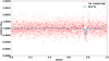 |
Fig. 1 Box Least Squares (BLS) detection of TOI-2427 b by the EXOTRANS pipeline. The light curve of the PDC-SAP flux measured by TESS, binned by approximately 10 minutes, and phase-folded at the period of 1.3067 d, shows a clear transit signal. |
2.1 TESS photometry
NASA’s TESS space telescope observed TOI-2427 in its 31st sector, between 22 October and 16 November 2020, using camera 2 and CCD 1, as part of its all-sky survey during the first year of the extended mission. The photometric data has a cadence of 120 s. We note that the star will be reobserved by TESS1 in sectors 105, 106, and 107 from June to August 2026.
The processing and calibration of the TESS target pixel files were conducted by the Science Processing Operations Center (SPOC; Jenkins et al. 2016) located at NASA Ames Research Center. The extraction of the light curve was performed by SPOC using simple aperture photometry (SAP; Twicken et al. 2010; Morris et al. 2020), followed by processing through the presearch data conditioning (PDC) algorithm, which uses a Bayesian maximum a posteriori approach to mitigate most instrumental artifacts and systematic trends (Smith et al. 2012; Stumpe et al. 2012, 2014). We downloaded the PDC-SAP TESS light curve of TOI-2427 from the Mikulski Archive for Space Telescope2 (MAST) and utilized it for the analyses presented in this paper. To assess potential contamination in the TESS aperture, we examined the contamination ratio (CROWDSAP keyword) provided in the TESS data products. The CROWDSAP value for TOI-2427 is 0.9998, indicating that 99.98% of the flux in the aperture originates from the target star itself, and that the contamination from nearby sources is negligible.
The Science Processing Operations Center searched the TESS sector 31 light curve for transit-like signals and, on 11 Dec. 2020, reported on the detection of a ∼ 550 ppm-deep transit signal occurring every 1.3 d on the TESS input catalog object (TIC; Stassun et al. 2018) 142937186. The planet candidate met all criteria of the automatic validation tests, such as those assessing odd-even transit depth variation and ghost diagnostic evaluations, and it was given the designation TOI-2427.01. We independently searched the TOI-2427 PDC-SAP light curve for transit signals using the EXOTRANS pipeline (Grziwa & Pätzold 2016), which employs a box least squares (BLS) algorithm (Kovács et al. 2006) to identify transit events. We significantly recovered the transit events detected by SPOC (Fig. 1) and did not identify any other significant transit signals.
In addition, we investigated the TESS light curve to search for rotational modulation, using the SAP flux from the Quick Look Pipeline (QLP; Huang et al. 2020), corrected with the Kepler Asteroseismic Data Calibration Software (KADACS; García et al. 2011). Applying the A2Z pipeline (Mathur et al. 2010; Ceillier et al. 2017; García et al. 2014), we found no significant rotation period below 10 d. However, the data revealed a possible long-period modulation (>21 d) that cannot be definitively constrained by the limited TESS coverage.
In 2021, high-resolution imaging, ground-based photometry, and reconnaissance spectroscopy were carried out to validate the planetary nature of the transit signal detected by TESS. These observations were analyzed using the validation tools TRICERATOPS and DAVE (Giacalone et al. 2022). The TRICERATOPS algorithm calculates the Bayesian probability that a candidate signal is an astronomical false positive (FP). The resulting FP probability for TOI-2427.01 was found to be below 1%, validating it as a planet with an orbital period of 1.3 d. The initial analysis by Giacalone et al. (2022) yielded the following planetary parameters for TOI-2427 b: an orbital period of ∼ 1.3 d, a radius of 1.80 ± 0.12 R⊕, a semimajor axis of 0.0202 ± 0.0002 AU, and an equilibrium temperature of 1117 ± 46 K.
However, because most exoplanets are detected using indirect techniques, objects identified by only a single indirect method are typically not considered confirmed. Another detection using a different technique is required to elevate the planet’s status from “validated” to “confirmed”, which is one of the aims of this paper.
2.2 WASP-South photometry
The ground-based Wide Angle Search for Planets survey in the southern hemisphere (WASP-South; Pollacco 2005) collected 123000 photometric data points of TOI-2427, from 2006 to 2014. During these observations, WASP-South was equipped with Canon 200 mm f/1.8 lenses and a broadband filter covering 400 – 700 nm. The setup included 2048 × 2048 CCDs with a plate scale of 13.7′′/pixel (Pollacco et al. 2006). Because we were unable to determine the exact stellar rotation period from TESS photometry alone owing to the relatively short baseline (Sect. 2.1), we applied the methods outlined by Maxted et al. (2011) to each year’s WASP light curves in order to search for periodic and quasi-periodic modulations caused by active regions corotating with the star. As representative examples, Fig. 2 shows periodograms from three different years, each covering about 150 nights.
The periodograms (Fig. 2, left-hand panels) show significant power at a period of 28 ± 1 d, and at its first harmonic (14 ± 1 d), with modulation amplitudes of up to 10 mmag. Since the 28-d period is close to the Moon’s orbital period, we verified that this signal was not due to moonlight contamination. This was performed by analyzing several neighboring stars in the same field, none of which show a similar 28-d modulation. Therefore, we conclude that the 28-d periodicity is intrinsic to TOI-2427. When folding the light curve data at the 28-d period, phase gaps remain due to WASP-South’s observation scheduling, which deliberately avoided the Moon to minimize potential contamination (Fig. 2, right-hand panels).
2.3 HARPS Doppler follow-up
In September 2021, we started an intensive Doppler follow-up of TOI-2427 using the High Accuracy Radial Velocity Planet Searcher (HARPS; Mayor et al. 2003) spectrograph mounted on the 3.6 m telescope of the European Southern Observatory (ESO), La Silla, Chile. The observations were performed as part of the high-precision radial velocity (RV) program3, carried out by the KESPRINT4 consortium with the HARPS spectrograph to spectroscopically confirm and determine the fundamental parameters of TESS transiting planets (see, e.g., Esposito et al. 2019; Fridlund et al. 2020; Luque et al. 2021; Serrano et al. 2022; Goffo et al. 2023; Osborne et al. 2024; Šubjak et al. 2025).
Over nearly six months, we acquired a total of 100 highresolution (R ≈ 115 000) HARPS spectra, each with an exposure time of 1800 s, and a median signal-to-noise ratio (S/N) of ∼ 67 per pixel at 550 nm, resulting in a total open-shutter time of 50 hours. The spectra were reduced using the dedicated HARPS data reduction software (DRS; Pepe et al. 2002; Lovis & Pepe 2007) available at the telescope. Absolute RV measurements were extracted by cross-correlating the Echelle spectra with a K5 binary mask (Baranne et al. 1996). The DRS provides three profile diagnostics of the cross-correlation function (CCF), namely the full width at half-maximum (FWHM), the bisector inverse slope (BIS), and the contrast.
We also used the codes TERRA (Anglada-Escudé & Butler 2012) and SERVAL (Zechmeister et al. 2018) to extract relative RV measurements, along with additional activity indicators, such as the Mount Wilson Ca II H & K S-index, the H α, the NaD1 & D2 indexes, the differential line width (dLW) and the chromatic index (crx). Both TERRA and SERVAL are based on template matching algorithms and have been proven to be better suited to derive precise RVs for M and K dwarfs than the CCF technique (see, e.g., Luque et al. 2021). Generally, there is no reason to prefer SERVAL over TERRA, since the results derived from both codes are consistent. However, for the analyses presented in this work, we used the relative RV dataset extracted with the SERVAL pipeline.
To spectroscopically confirm the planetary nature of the 1.3d transit signal detected by TESS, we started by performing a frequency analysis of the HARPS SERVAL RV measurements, CCF profile diagnostics, and activity indicators. This analysis also provides an opportunity to detect additional signals induced by other planets and/or stellar magnetic activity. For this purpose, we used the generalized Lomb-Scargle (GLS) periodogram (Lomb 1976; Scargle 1982; Zechmeister & Kürster 2009) and assessed the significance of a given signal by estimating its false alarm probability (FAP). The latter is defined as the probability that noise may produce a power greater than the power of a given signal detected in the periodogram of the data, within a certain frequency range (Hatzes 2019). Following Murdoch et al. (1993) and Kuerster et al. (1997), we determined the FAP using the bootstrap method by randomly shuffling the HARPS data 106 times, while keeping the time stamps fixed. A peak was deemed significant if its bootstrap FAP was less than 0.1%.
During the analysis of the HARPS SERVAL RV time series, we used the pre-whitening procedure to iteratively identify significant signals in the periodogram of the Doppler time series and remove them from the RV time series via a fit with sinusoidal functions (see, e.g., Hatzes et al. 2010). At each step of the process, when a significant peak was detected in the periodogram of the RV data, we kept its frequency fixed to that identified in the power spectrum and fitted for the amplitude, phase, and offset. The best fitting sine curve was then subtracted from the time series, and the periodogram of the residuals was recomputed. This process was iteratively repeated to identify additional significant signals in the Doppler time series until the noise level was reached, i.e., until none of the peaks have a power greater than the power corresponding to our FAP threshold of 0.1%.
The first panel of Fig. 3 shows the GLS periodogram of the HARPS SERVAL RVs in the frequency range 0.0 – 1.0 d−1. The highest peak is found at fb ≈ 0.766 d−1, corresponding to a period of Pb ≈ 1.306 d, which matches the transit period detected by TESS. We note the presence of the 1−d alias at 1− 0.766=0.234 d−1, as well as the presence of symmetric peaks with respect to half the median sampling frequency at 0.5 d−1. That itself is attributed to the 1-d data sampling. The signal at fb does not have a counterpart in the periodograms of the activity indicators and CCF profile diagnostics, as shown in Fig. 4. Although its false alarm probability (FAP) is 0.16%, i.e., higher than our significance threshold level (FAP=0.1%), the detection of a peak at a known frequency strongly suggests that this signal is due to TOI-2427 b.
To quantitatively reassess the significance of the TOI-2427 b’s RV signal, the FAP was estimated at the known frequency fb ≈ 0.766 d−1. Following the windowing bootstrap method described in Hatzes (2019), the false alarm probability was first estimated over a 0.1-d−1-wide window centered around fb, and then the window was iteratively narrowed down by 0.01 d−1 for nine times, with the FAP being recomputed at each step. The fit to FAPs versus window sizes, extrapolated to the intercept (that is, the zero window length), yields a FAP < 0.001% at fb, spectroscopically confirming the transit signal detected by TESS.
The periodogram of the HARPS RV residuals, after subtracting the Doppler reflex motion induced by the transiting planet TOI-2427 b, displays a significant peak at frot=0.036 d−1 (Prot ≈ 28 d) with a FAP < 0.1% (Fig. 3, second panel). A similar peak is detected in the power spectra of most activity indicators and CCF profile diagnostics, the signal being significant (FAP < 0.1%) in the dLW, Na D1, and Na D2 (Fig. 4). We note that this signal is consistent with the periodic photometric modulation of 28 ± 1 d independently detected in the WASP-South photometry (Sect. 2.2).
After removing the 28-d signal, a third significant peak was identified at fc=0.194 d−1 (Pc ≈ 5.15 d), with an amplitude of about 3.6 m s−1 and a FAP < 0.1% (Fig. 3, third panel). This signal remains undetected in the periodograms of the activity indicators and CCF profile diagnostics (Fig. 4), suggesting that it is likely due to the presence of a second low-mass planet in the system, hereafter referred to as TOI-2427 c.
A further iteration of the pre-whitening procedure led to the detection of a significant peak at 2 × frot ≈ 0.071 d−1 (Prot/2 ≈ 14 d), which is the first harmonic of frot (Fig. 3, fourth panel). This signal is also found in the WASP-South photometry (Sect. 2.2) and is significantly detected in the periodograms of the dLW and BIS (Fig. 4). Given the spectral type of the star (K 7 V), the 28−d and 14−d signals are very likely caused by the presence of spots and plages carried around by stellar rotation (see, e.g., McQuillan et al. 2014). The 28-d signal was interpreted as the rotation period of the star. The 14−d period peak is likely a signature of inhomogeneities in spot coverage of the stellar photosphere in combination with visual effects at the stellar limb (see, e.g., Vanderburg & Johnson 2014). No additional significant signals were detected in the RV residuals (Figure 3, lower panel).
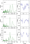 |
Fig. 2 Periodograms of the WASP-South data for TOI-2427, showing strong peaks at the 28-d rotational period and its 14-d first harmonic. The horizontal line is the estimated 1% false-alarm probability. The right-hand panels show the data folded at the rotational period of 28 d. |
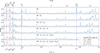 |
Fig. 3 Generalized Lomb-Scargle periodograms of the HARPS SERVAL Doppler measurements and residuals. From top to bottom: RV data (upper panel); RV residuals following the subtraction of the Doppler signal of TOI-2427 b (second panel), TOI-2427 b plus the star rotation signal at 28 d (third panel), TOI-2427 b & c plus the star rotation signal at 28 d (fourth panel), TOI-2427 b & c plus the star rotation signals at 28 and 14 d (lower panel). The horizontal dotted lines mark the FAP at 0.1%, as derived using the bootstrap method. The vertical dashed blue and green lines mark the orbital frequencies of TOI-2427 b and c, respectively. The vertical dashed red lines mark the stellar rotation frequency at 1/28=0.036 d−1 and its first two harmonics (1/14=0.071 d−1. and.1/9.3=0.108 d−1). |
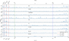 |
Fig. 4 Generalized Lomb-Scargle periodograms of the HARPS CCF profile diagnostics and activity indicators. From top to bottom: BIS (upper panel); FWHM (second panel), contrast (third panel); crx (fourth panel); dLW (fifth panel); Hα (sixth panel); S-index (seventh panel); Na D1 (eighth panel); Na D2 (lower panel). The horizontal dotted lines mark the FAP at 0.1%, as derived using the bootstrap method. The vertical dashed blue and green lines mark the orbital frequencies of TOI-2427 b and c, respectively. The vertical dashed red lines mark the stellar rotation frequency at 1/28=0.036 d−1 and its first two harmonics (1/14=0.071 d−1 and 1/9.3=0.108 d−1). |
3 The host star TOI-2427
The main identifiers and equatorial coordinates, along with the proper motion, parallax, absolute radial velocity, and optical and infrared magnitudes of the host star TOI-2427 (CD-31 1415) are listed in Table 1. With a distance of ∼ 25.6 pc (Gaia Collaboration 2023), TOI-2427 is one of the Sun’s closest neighbors. It has an apparent visual magnitude of V=10.385 ± 0.018 (Henden et al. 2015), which makes the star relatively bright and thus amenable to detailed follow-up observations, including highprecision radial velocities.
We start with the determination of the fundamental parameters of the host star in Sect. 3.1. We then derive its age in Sect. 3.2, and discuss its galactic population membership in Sect. 3.3.
3.1 Host star photometric parameters, radius, and mass
To determine the photospheric parameters needed for deriving the stellar mass, radius, and age of the star, we analyzed the co-added high-resolution (R ≈ 115 000) HARPS spectrum, which has a signal-to-noise (S/N) ratio per pixel at 550 nm of ∼ 600. We used two different methods: Spectroscopy Made Easy5 (SME; Valenti & Piskunov 1996; Piskunov & Valenti 2017) and the SpecMatch-Emp software (Yee et al. 2017). SME computes synthetic spectra based on atomic and molecular line data from VALD3 (Ryabchikova et al. 2015) and fits them to the observed spectrum to determine the photospheric parameters. SpecMatch-Emp compares the observed spectrum with template spectra of well-characterized FGKM stars. For the SME modeling, we chose the MARCS model atmosphere (Gustafsson et al. 2008) and checked our results against the Atlas 12 atmosphere grid (Kurucz 2013). We fixed the macro- and micro-turbulent velocities (vmac and vmic) to 1.5 km s−1 and 0.5 km s−1, respectively (Gray 2008), and refer to Fridlund et al. (2017) and Persson et al. (2018) for a detailed description of the modeling schematic. From the SME analysis, we found an effective temperature of Teff=4203 ± 110 K, a surface gravity of log g*=4.62 ± 0.12 (cgs), iron and calcium abundances of [Fe/H]=−0.210 ± 0.093 and [Ca/H]=−0.160 ± 0.088, respectively, and a projected rotational velocity of v sin i*=2.80 ± 0.93 km s−1 (Table 1). The SME and SpecMatch-Emp results are in good agreement within 1.0 – 1.5 σ, as shown in Table 2.
Main identifiers, equatorial coordinates, optical and infrared magnitudes, and fundamental parameters of CD-31 1415.
Comparison table of the TOI-2427 spectroscopic parameters derived with SME (first row), SpecMatch-Emp (second row), and astroARIADNE (third row). The last row reports the effective temperature retrievied from Gaia DR2 (Gaia Collaboration 2018).
We derived the stellar radius with the spectral energy distribution (SED) fitting software astroARIADNE6 (Vines & Jenkins 2022) using spectroscopic priors from the analysis we performed with SME (Table 2). We utilized the Gaia DR3 parallax together with photometry from the following bandpasses (Table 1): Johnson B and V (APASS; Henden et al. 2015); G, GBP, GRP (Gaia DR3; Gaia Collaboration 2023); J, H, Ks (2MASS; Cutri et al. 2003), W1 and W2 (AllWISE; Cutri 2014). astroARIADNE uses four different atmospheric models from BtSettl (Allard et al. 2012) and Phoenix v2, one of which is shown in Fig. 5 together with the spectroscopy and computes the final radius with Bayesian Model Averaging based on the relative probabilities of each model, taking into account different model-specific systemic biases (Fragoso et al. 2018; Vines & Jenkins 2022). To be conservative, we chose the errors computed with a sampling method as described in Vines & Jenkins (2022). The final stellar radius was found to be  . The stellar mass was computed by astroARIADNE interpolating on the MIST (Choi et al. 2016) isochrones and was found to be
  . The stellar luminosity is L*=0.110 ± 0.012 L⊙, and the visual extinction is consistent with zero (
 ). All our results are listed in Table 1.
For completeness, in Table 2 we report the effective temperature from Gaia DR2 (Gaia Collaboration 2018), along with results extracted from the posterior distributions of the astroARIADNE SED modeling. The effective temperature and surface gravity of the star are indicative of a K7 V spectral type (Pecaut et al. 2012; Pecaut & Mamajek 2013), with standard values7 for mass and radius being roughly 0.64 M⊙ and 0.63 R⊙, respectively, in very good agreement with our results.
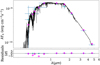 |
Fig. 5 Spectral energy distribution (SED) of TOI-2427. This figure displays the model with the highest probability from Allard et al. (2012, BT-Settl) in black. The magenta colored diamonds and the blue points mark the synthetic and the observed photometry, respectively. The 1σ uncertainties are shown with vertical error bars; the horizontal bars mark the effective width of the bandpasses. The residuals are normalized to the errors of the photometry. |
3.2 Stellar age
We estimated the age of TOI-2427 using various methods. Isochrone fitting (PARAM; da Silva et al. 2006), based on the stellar parameters listed in Table 2, yields a poorly constrained age estimate of 6.7 ± 6.0 Gyr. For main-sequence stars with temperatures cooler than the Sun, isochrones can be degenerate, making precise age determinations challenging (Lachaume et al. 1999).
To refine this estimate, we searched the HARPS co-added spectrum for additional age indicators. Lithium (Li) abundance was found to be fully depleted, with an upper limit of log N(Li) < −0.5, suggesting that the star is at least 500-Myrold (Soderblom 2010). The  index, a measure of chromospheric activity extracted from the Ca II H & K lines, was found to be −4.86 ± 0.06, indicating a moderate level of activity. Using the empirical relation from Suárez Mascareño et al. (2015),
  implies a rotation period of ∼ 24 d, which is consistent with the periodicity detected in the WASP-South photometry (Sect. 2.2) and HARPS activity indicators (Sect. 2.3).
Using the derived 28 ± 1 d stellar rotation period as a starting point for the empirical period-age relation (Suárez Mascareño et al. 2015), we derived an age of approximately  , whereas the calculated upper limit is, in fact, even higher but limited by the 13.8 Gyr age of the universe. This relation provides reliable estimates for stars older than 1.5 Gyr, but becomes less constrained for early M-type and cooler K-type stars. Given the limitations of current methods, we emphasize that age determinations for such stars inherently carry significant uncertainties.
Although the star is classified as a K-type star, it’s effective temperature is not much higher than that of M-type stars. Therefore, we also applied the rotation-age relationship from Engle & Guinan (2023) for hotter M-type stars, which yields an age of 1.58 ± 0.14 Gyr. This estimate matches the younger end of the age range from the Suárez Mascareño et al. (2015) relation. As a result, the system is likely to be on the younger side within the given uncertainties.
3.3 Galactic population membership
The measured [Fe/H] and age for this star (Table 1) could place the star within the age and metallicity distributions of either the galactic thin- or thick-disk. To investigate the galactic stellar population membership of TOI-2427, we applied the techniques of Reddy et al. (2006) to compute the U, V, W stellar LSR velocities. Using Gaia DR3 astrometric measurements and absolute radial velocity (Gaia Collaboration 2023), we computed U=−28.25 ± 0.07 km s−1, V=−20.31 ± 0.06 km s−1, W=−18.55 ± 0.10 km s−1, and P(thin disk)=0.9874 ± 0.005, P(thick disk)=0.0126 ± 0.0001, and P(halo)=0.0002 ± 0.0001. Thus, TOI-2427 is firmly established as a kinematic member of the galactic thin disk. This is further supported by the stellar [Ca/H] measurement failing to show any enhancement of this alpha-capture element.
4 Planetary characterization
To determine the parameters of the two planets orbiting TOI-2427, we modeled the HARPS SERVAL RV measurements, first alongside two of the activity indicators (Sect. 4.1) and then jointly with the TESS transit light curves (Sect. 4.2). Lastly, we investigated the long-term stability of the system in Sect. 4.3. As a basis for the analysis of the system, we adopted the stellar parameters derived in Sect. 3 and listed in Table 1.
4.1 Radial velocity modeling
We used the software suite pyaneti (Barragán et al. 2019, 2022a) to derive the planetary parameters. pyaneti is based on Bayesian statistics combined with Markov chain Monte Carlo (MCMC; Brooks et al. 2011) sampling to explore the parameter space of planetary systems. One of the key features of the code is its built-in multidimensional Gaussian process (GP) approach to jointly model radial velocity and activity indicator time series (Rajpaul et al. 2015).
The HARPS RVs and activity indicators display periodic and quasi-periodic variations at the stellar rotation period (∼ 28 d) and its first harmonic (∼ 14 d; see Sect. 2.3). The same signals are also significantly detected in the WASP-South light curve (Sect. 2.2) and are ascribable to the presence of active regions combined with stellar rotation. To account for the Doppler signal induced by stellar activity, we applied the multidimensional GP approach, as implemented in pyaneti. Briefly, we modeled the HARPS SERVAL RVs along with the time series of the activity indicators, assuming that the same function G(t) can describe both sets of data. This function G(t) represents the projected area of the visible stellar disk covered by active regions at a given time. For the analysis of the TOI-2427 HARPS data, we selected the two activity indicators that show the strongest power in their periodograms, namely dLW and Na D2, and modeled them alongside the RVs. We used a three-dimensional GP defined as:
 (1)
(1)
 (2)
(2)
 (3)
(3)
where the amplitudes ARV, BRV, AdLW, and ANaD2 are coefficients that relate G(t) to the observables. We modeled the HARPS SERVAL RV measurements as a function of G(t) and its time derivative , since both depend on the fraction of the stellar surface covered by active regions and how these regions evolve over time on the disk. The signal of the activity indicators, on the other hand, almost exclusively depends on the size of the active regions and can therefore be modeled using only G(t) (Rajpaul et al. 2015). We used the following quasi-periodic kernel:
![Mathematical equation: $\gamma\left(t_{i}, t_{j}\right)=\exp \left[-\frac{\sin ^{2}\left[\pi\left(t_{i}-t_{j}\right)/P_{\mathrm{GP}}\right]}{2 \lambda_{\mathrm{p}}^{2}}-\frac{\left(t_{i}-t_{j}\right)^{2}}{2 \lambda_{\mathrm{e}}^{2}}\right].$](/articles/aa/full_html/2025/07/aa52620-24/aa52620-24-eq23.png) (4)
(4)
The hyper-parameters in Eq. (4) are:
PGP, the characteristic period of the GP, interpreted as Prot;
λp, the inverse of the harmonic complexity;
λe, the long-term evolution timescale of active regions.
We performed multidimensional GP regression under two different scenarios. For the first scenario, we modeled the HARPS time series assuming that the only two signals present in the data are those due to stellar activity and the validated transiting planet TOI-2427 b. The periodogram of the RV residuals – after subtracting the median derived model of the fitted parameters — shows a significant power at 5.15 d, in agreement with the results presented in Sect. 2.3. Consequently, we added a second Keplerian to account for the Doppler reflex motion induced by the second planet. pyaneti computes two model selection metrics, the Bayesian information criterion (BIC) and the Akaike information criterion (AIC). We compared BIC and AIC for the one-planet and two-planet models. The single-planet model provides a BIC of −17772.8 and an AIC of −17 892.9, while the two-planet model calculates a BIC equal to −17809.7 and an AIC of −17 946.1. In pyaneti, lower values of BIC and AIC indicate a more favorable model. We find that Δ BIC=36.9 and Δ AIC=35.8, both of which comfortably exceed the usual threshold of 10 (Liddle 2007). Moreover, the power spectra of both the activity indicators and the CCF profile variation diagnostics reveal no significant signals at 5.15 d. Together, these results provide compelling evidence for the presence of TOI-2457 c.
4.2 Radial velocity and light curve joint analysis
We used the code pyaneti to model the TESS transit light curves from sector 31 together with the HARPS SERVAL RV measurements and the dLW and NaD2 activity indicators. The TESS data included in the analysis are 2.5−hr segments of the PDC-SAP light curve centered around the respective transits. We detrended each segment of the light curve by fitting a second-order polynomial to the out-of-transit data.
The RV model includes two Keplerians to describe the Doppler reflex motions induced by TOI-2427 b and c, and the GP model presented in Sect. 4.1 to account for the activity-induced signals. The eccentricity (e) and the argument of periastron (ω*) of the stellar orbit were modeled following the parametrization proposed by Anderson et al. (2010), i.e.,  and
and  . We fitted the TESS transits of TOI-2427 b with the limb-darkened quadratic model of Mandel & Agol (2002) and followed the Kipping (2013)’s parametrization q1 and q2 for the linear and quadratic limb-darkening coefficients u1 and u2. We constrained u1 and u2 using Gaussian priors on q1 and q2 based on the values derived by Claret (2017) for the TESS passband, imposing conservative error bars of 0.1 (Table 3). We fitted a photometric and an RV jitter term to account for any instrumental noise not captured by the nominal uncertainties and possible sources of Doppler variations (e.g., stellar activity and/or additional planets) not included in our RV model. We sampled the stellar density ρ* using a Gaussian prior on the stellar mass and radius, as derived in Sect. 3 (see Table 1), and recovered the scaled semimajor axis via Kepler’s third law. For all the remaining parameters, as well as for the multidimensional GP hyper-parameters and amplitudes (Sect. 4.1), we adopted uniform priors and added a jitter term to the diagonal of the covariance for each time series.
We sampled the parameter space with 500 Markov chains and created the posterior distributions using the last 5000 iterations of the converged chains with a thin factor of 10, leading to a distribution of 250000 data points for each sampled parameter. The posterior values for the modeled parameters, along with their priors, and derived parameters are listed in Tables 3 and 4, respectively. For each parameter, the estimated value and its uncertainty are defined as the median and the 68.3% region of the credible interval of the marginalized parameter distribution, respectively. Figure 6 displays the time series of the HARPS SERVAL RVs, dLW, and Na D2 activity indicators, along with the median models and the 68.3% and 95.5% credible intervals. Figures 7 and 8 show the RV curves of TOI-2427 b and c phase-folded at the orbital period of the two planets, once the other Doppler signals have been removed. The phase-folded transit light curve of TOI-2427 b and the median model are shown in Fig. 9.
The HARPS RVs provide a semi-amplitude of Kb=4.47 ± 0.39 m s−1 for the ultra-short period planet TOI-2427 b, which yields a planetary mass of  (∼9% relative precision). From the modeling of the TESS transit light curves we derived a planetary radius of
  . The mass and radius imply a mean bulk density of
  , with an overall precision of ∼ 25%. For the outer planet at 5.15 d (TOI-2427 c), we measured an RV semi-amplitude variation of
  , which translates into a minimum mass of
  . We found that the eccentricities of both planets are consistent with zero within less than 1.5 σ (Table 4), as expected given the compact architecture of the planetary system (Weiss et al. 2023).
Our results reveal that the GP period of  effectively characterizes the rotation period of the star, as it is consistent with the result of the WASP-South photometric time series (Prot=28 ± 1 d). The hyper-parameter
  is comparable to PGP, suggesting that the same active regions on the stellar photosphere survive for slightly more than one stellar rotation. The inferred hyper-parameter
  suggests a high degree of harmonic complexity inherent to the underlying mechanisms that govern the stellar signal (Barragán et al. 2022b). This finding indicates the existence of multiple groups of active regions on the stellar photosphere, which would contribute to the complex patterns observed in our spectroscopic time series (Fig. 6).
Based on the parameters we obtained for the two planets, we considered performing a transit timing variation (TTV; see, e.g., Korth et al. 2023) analysis, as this method can often be used in resonant systems. However, even though the planets are in a 4:1 period commensurability, in this case a TTV analysis was deemed not applicable, since TOI-2427 was observed in only one TESS sector at the time of writing. This means that there were not enough observations to perform a meaningful TTV analysis.
Model parameters of the transit and RV joint analysis of TOI-2427 b and c.
4.3 Dynamical analysis
While a TTV analysis is not possible due to the insufficient monitoring of planet b with TESS, the 4: 1 near-resonant configuration of both planets renders the TOI-2427 planetary system highly intriguing for a detailed dynamical analysis. To determine the dynamical stability of the solution presented in Table 4 we employed the Reversibility Error Method (REM; Panichi et al. 2017), which has been shown to be a close analog of the Maximum Lyapunov Exponent (MLE). In the analysis of multi-body systems, it relies on numerical integration schemes that are time-reversible, in particular symplectic algorithms. This method is based on the calculation of the difference between the initial-state vector and the final-state vector, which is obtained by integrating the system of equations at a specific time and returning to the initial epoch. The difference thus defined will depend on the dynamic nature of the system.  or
or  means that the difference reaches the size of the orbit.
We tested the dynamical stability of the solution using the whfast integrator with the 17th order corrector (with a fixed time step of 0.08 d) as implemented within the REBOUND package (Rein & Liu 2012; Rein & Spiegel 2015) for 50 000 orbital periods of the farthest planet. As illustrated in Fig. 10, we obtained  , indicating that the solution is stable. The ± 3 σ uncertainty of the orbital period of planet c, placed on the dynamical map, shows a safe distance from the 4: 1 resonant structure. The additional information about the ± 3 σ eccentricity uncertainty in the model with the eccentricities set as free parameters is consistent with the results of the circular model. The set of initial conditions used for the analysis describing the TOI-2427 system represents a non-resonant case.
Derived parameters for the TOI-2427 planetary system.
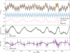 |
Fig. 6 Time-series of the HARPS SERVAL RV measurement (upper panel, orange circles), dLW (middle panel, green circles), and Na D2 (lower panel, violet circles). The thick lines mark the models as derived from the medians of the marginalized distributions of the inferred parameters. The dashed gray areas mark the 68.3%(1 σ) and 95.5%(2 σ) credible intervals. |
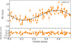 |
Fig. 7 HARPS radial velocity curve for TOI-2427 b phase-folded at a period of 1.3 d, along with the model derived from the medians of the marginalized posterior distributions of the inferred Keplerian parameters (thick line). |
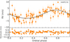 |
Fig. 8 HARPS radial velocity curve for TOI-2427 c phase-folded at a period of 5.15 d, along with the model derived from the medians of the marginalized posterior distributions of the inferred Keplerian parameters (thick line). |
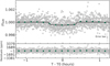 |
Fig. 9 TESS transit light curve phase-folded at the orbital period of TOI-2427 b (gray dots), 10−min binned light curve (green dots), and model derived from the medians of the marginalized posterior distributions of the inferred transit parameters (thick line). |
5 Results
Here, we present our results with a focus on planetary and orbital parameters, including the bulk density as a basis for classification (Sect. 5.1). The interior structure of the transiting planet TOI-2427 b is examined in Sect. 5.2. We explore possible atmospheric compositions and escape processes in Sect. 5.3, and discuss prospects for atmospheric characterization in Sect. 5.4.
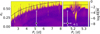 |
Fig. 10 Dynamical map for the solution presented in Table 4 for a wide range of orbital periods and eccentricities of the outer non-transiting planet c. The narrow right panel presents a close-up of the scan for the 3 σ region around the orbital period of the planet c in the circular model (black filled circle with a white rim) and for the 3 σ region around the orbital period and eccentricity of planet c in a model with eccentricities as free parameters (filled black square with white rim). Small values of the fast indicator |

5.1 Planetary parameters
Planet b has a high density of  , indicating that it is primarily composed of rock and iron. Figure 11 displays the position of TOI-2427 b in the mass-radius diagram, along with those of known transiting exoplanets8. The solid and dashed lines mark different composition models from Zeng et al. (2016). TOI-2427 b falls within the expected range for planets with a significant iron and rock composition, and its position is comparable to that of an Earth-like composition within the 1σ uncertainty level.
Given that the RV method provides only the minimum mass Mc sin ic for TOI-2427 c (Table 3), we estimated the true mass under the assumption that the planet’s orbit is coplanar with that of TOI-2427 b. This assumption is reasonable for compact systems like TOI-2427, since most are coplanar (Fang & Margot 2012; Weiss et al. 2023). The maximum inclination that planet c can have to avoid producing transit events is calculated by imax = arccos (R*/ac)=86.57 ± 0.19 deg, which exceeds by ∼4 deg the measured orbital inclination of planet  ). Therefore, a coplanar scenario would account for the non-transiting nature of planet c. This suggests that the true mass of TOI-2427 c is likely close to the measured minimum mass of
  , which could mean that the planet is a member of the small sub-Neptune category.
We assumed that the planets are coplanar to estimate the radius of TOI-2427 c. We used the inferred mass and applied the probabilistic forecasting tool Forecaster (Chen & Kipping 2017), which estimates the radius of planet c at  . The colored area in Fig. 11 marks the possible position of TOI-2427 c in the mass-radius diagram.
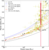 |
Fig. 11 Mass-radius diagram showing the positions of TOI-2427 b (red dot) along with all exoplanets alongside all exoplanets with mass and radius measurements known to within 30% relative precision or better (yellow points with error bars; source: NASA Exoplanet Archive), and solar system planets (colored dots). The light-red region denotes the minimum mass of TOI-2427 c, and the darker red region indicates its statistically inferred radius range from Forecaster when assuming coplanar orbits with planet b. Composition models (solid and dashed lines) are taken from Zeng et al. (2016). |
5.2 Interior structure
To derive possible interior structures and compositions for the inner planet TOI-2427 b, we used the interior structure model described in Brugger et al. (2016, 2017); Acuña et al. (2021). This forward interior structure model solves a set of differential equations to obtain the pressure, temperature, density, and gravity as a function of the planetary radius, which is represented by a one-dimensional grid. The interior structure is divided into three layers: a Fe-rich core, a mantle dominated by silicate compounds (including enstatite MgSiO3), and a hydrosphere. Then, we performed a retrieval of the observed mass and radius from Table 4 with an adaptive MCMC (Dorn et al. 2015; Director et al. 2017; Acuña et al. 2023) for an efficient sampling of the compositional parameters. Rocky planets that may present a thin volatile layer tend to be compatible within uncertainties with the pure MgSiO3 composition curve in the mass-radius diagram (Fig. 11). For rocky planets in this region of the mass-radius diagram, a degeneracy exists between the core and envelope mass fractions. TOI-2427 b is denser than a pure MgSiO3 planet, which means that it likely has no volatiles and has a significant iron content. Therefore, in the analysis of the interior structure of TOI-2427 b, the water mass fraction (WMF) was constant and set equal to zero. The other compositional parameter in our interior model, the core mass fraction (CMF), was the only free parameter in our retrieval. The retrieval was then performed considering the planetary mass and radius as observables (see Table 4).
Fig. 12 shows the corner plot of the posterior distribution functions of the parameters. TOI-2427 b presents an iron-to-silicon mole ratio of  and a CMF 1σ confidence interval ranging from 24% to 74%, which is compatible with both the Fe content of Earth (CMF=0.32) and that of Mercury (CMF=0.68). This range in CMF is partially compatible with the CMF distribution of a sample of super-Earths obtained from a similar MCMC interior analysis, whose typical CMF spans between 10% and 50% (Plotnykov & Valencia 2020). Hence, we can conclude that TOI-2427 b is most likely a super-Earth with no volatiles, although the possibility that it could be a super-Mercury (CMF > 0.68) cannot be completely ruled out.
We considered a similar analysis for planet c, but, due to the large uncertainties associated with having only an estimation of its radius, this analysis was deemed not to provide convincing results. Breaking this degeneracy would require an independent constraint on the planet’s radius, which is challenging for a non-transiting planet. However, future improvements in empirical mass-radius relations or secondary eclipse measurements might offer insights into its size and composition.
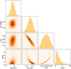 |
Fig. 12 Corner plot of the planetary parameters retrieved by our MCMC analysis on the interior structure of TOI-2427 b. |
5.3 Possible atmospheric escape
Given the high equilibrium temperature of TOI-2427 b (Table 4), it is very likely that any gas with low molecular weight (such as H2 or He) has escaped. This is the case for Earth, where the lack of hydrogen and helium in the atmosphere is attributed to Jeans escape (Jeans 1926). Since TOI-2427 b is compatible with an Earth-like interior, the restricted Jeans escape parameter was computed as Λp=Rp/H (Fossati et al. 2017), where H is the scale height of the planet’s atmosphere. It was found that Λp=29 ± 7, a value comparable to the Jeans escape parameter of Earth: Λ⊕=27. However, the Jeans escape rate for the Earth is very low, and can only impact the composition of extremely thin atmospheres.
A more efficient mechanism to remove primordial H2-He gas is photoevaporation, i.e., the loss by X-ray and extreme ultraviolet (XUV) driven stellar winds. To analyze this hypothesis, we evaluated theoretical atmospheric escape rates for TOI-2427 b. The photoevaporation mass-loss rate from the atmosphere in the energy-limited regime is (Erkaev et al. 2007; Owen & Wu 2013):
 (5)
(5)
where FXUV is the XUV flux received by the planet, G the gravitational constant, and ε is an efficiency parameter. The XUV flux from the star is not constant in time, and its value was approximated by the analytical fit obtained by (Sanz-Forcada et al. 2011). Furthermore, ε ∼eq 0.05 from (Owen & Jackson 2012) was estimated. The XUV flux is decreasing in time, which means that most of the photoevaporation happens during the first Gyr of the planet’s evolution. Following the approach of Aguichine et al. (2021), we estimate the total mass of H/He lost by photoevaporation by integrating the mass-loss rate  , assuming that Mp, Rp, and Teq remained roughly constant and that only the XUV flux decreased during the evolution of the planet. We found that TOI-2427 b could have lost ∼ 0.10 M⊕ of H/He, i.e., ∼ 1.9% of its initial mass. The initial amount of hydrogen can be estimated by theoretical predictions; giving a value of ∼ 0.5% (Ginzburg et al. 2016). This suggests that any primordial hydrogen is lost from the atmosphere of TOI-2427 b. Our results are in line with the findings of Rogers et al. (2023), who use a more elaborate photoevaporation model than the simple prescription presented here.
Heavier molecules such as H2O can also be subject to photoevaporation, but the efficiency of the process is a few orders of magnitude lower (Ito & Ikoma 2021), making the problem extremely fine-tuned. In addition to that, it should be noted that only a pure helium atmosphere would have a non-negligible size when compared to the planetary radius: H/Rp ≃ 0.85%. Therefore, our conclusion is that TOI-2427 b has either no atmosphere or a thin secondary atmosphere made of gas with a high mean molecular weight such as H2O, N2 or CO2.
5.4 Prospects for atmospheric characterization of TOI-2427 b
In order to assess the viability of characterizing the atmosphere of TOI-2427 b with the JWST, we calculated the transmission spectroscopy metric (TSM) and the emission spectroscopy metric (ESM) as defined by Kempton et al. (2018). With a radius of  , TOI-2427 b is situated precisely at the border of two classes of planets defined by Kempton et al. (2018) as Terrestrials (Ter; Rp < 1.5 R⊕) and Small sub-Neptunes (SSN; 1.5 < Rp < 2.75 R⊕). Consequently, we calculated the TSM and ESM of TOI-2427 b for both scenarios using planet radius values with 1 σ above and below the nominal value presented in Table 4. For the Terrestrial scenario, this value is Rb=1.5 R⊕, while for the Small sub-Neptune scenario, it is Rb=1.7 R⊕. The remaining planetary parameters used for the calculation of TSM and ESM in both scenarios are identical and were retrieved from Table 4 (Mb and Teq). The stellar parameters, namely the near-infrared magnitudes J and Ks, the effective temperature Teff, and the stellar radius R*, were drawn from Table 1. In the case of the Small sub-Neptunes scenario, we obtained TSMSSN=79 ± 20 and ESMSSN=15.7 ± 2.5. In the Terrestrials scenario, the corresponding values are TSMTer=8.1 ± 2.3 and ESMTer=12.2 ± 2.1. Given that Kempton et al. (2018) propose a threshold of TSM > 10 and ESM > 7.5 for Terrestrial planets and a threshold of TSM > 90 for Small sub-Neptunes, the atmospheric characterization of TOI-2427 b using transmission spectroscopy would present a significant challenge for JWST. Nevertheless, with an ESM value exceeding 7.5, TOI-2427 b represents a compelling target for atmospheric characterization through emission spectroscopy.
6 Summary and conclusions
In this paper, we present an intensive high-precision Doppler follow-up of the K7 dwarf star TOI-2427 carried out with the HARPS spectrograph. We spectroscopically confirmed the transiting planet TOI-2427 b, which was previously validated by Giacalone et al. (2022). We jointly modeled the HARPS RV measurements and TESS transit light curves to derive the fundamental parameters of the planet. Our work provides precise determinations of the planetary mass, radius, and mean density, along with detailed information on the possible internal structure and atmospheric escape of the planet. We also discovered an additional periodic signal in the HARPS RV data associated with the presence of a second low-mass planet, TOI-2427 c.
We find that TOI-2427 b has a mass of  , a radius of
  , and a high mean density of
  , consistent with a rocky, iron-rich super-Earth. This planet orbits extremely close to its host star, with a semimajor axis of ∼ 0.02 AU and an orbital period of ∼ 1.3 d. Although ultra-short-period (USP) planets are typically defined as those with orbital periods shorter than one day, the period of TOI-2427 b places it just above the 1-d limit. Nonetheless, its high density and proximity to the star are reminiscent of USP planets, aligning with previous findings suggesting that many USP planets have an Earth-like composition and that they are not fundamentally distinct from planets with slightly longer orbital periods (Dai et al. 2018; Deeg et al. 2023).
Due to its proximity to the star, TOI-2427 b is likely tidally locked and experiences intense stellar irradiation, resulting in an equilibrium temperature exceeding 1100 K (Table 4). This extreme environment may sustain molten rock on the dayside, forming a partial magma ocean (Dorn & Lichtenberg 2021; Boukrouche et al. 2021). The high radiation flux (Table 4) also makes it unlikely that the planet can retain a stable primary atmosphere. However, heavier gases such as C2 O and N2 could form a secondary atmosphere, similar to those of Venus or Mars. Comparisons with other tidally locked planets, such as those in the TRAPPIST-1 and K2-141 systems (Greene et al. 2023; Zieba et al. 2022), suggest that detecting such an atmosphere would be challenging due to the small scale heights involved (Sect. 5.3).
Our derived parameters place TOI-2427 b near the lower boundary of the so-called Neptune desert, a region in the mass-period parameter space where Neptune-sized planets are notably scarce, which is probably due to significant atmospheric loss induced by intense stellar irradiation (Mazeh et al. 2016; Castro-González et al. 2024). The location of the planet at the edge of this desert suggests that it may once have possessed a more substantial envelope that was stripped away, leaving behind a dense, rocky core. As such, TOI-2427 b represents an intriguing target for investigating both atmospheric erosion processes and planet formation pathways within this sparsely populated region.
In addition to the detailed characterization of planet b, we discovered the presence of a second planet in the system, namely TOI-2427 c, with an orbital period of ∼ 5.15 d and a minimum mass of ∼ 6.5 M⊕. The analysis of the TESS light curve revealed the absence of transit signals from the second planet, preventing measurements of its radius and therefore its true mass. Given that the two planets are likely coplanar, we infer that the minimum mass of TOI-2427 c is probably close to the true mass of the planet. A statistical estimate of its size suggests a radius of 1.9-3.8 R⊕ (1 σ confidence interval) that possibly places it above the radius valley, which lies at ∼ 2 R⊕ for a period of ∼ 5 d (Fulton et al. 2017; Van Eylen et al. 2018).
With a harmonic period ratio of 4:1, TOI-2427 b and c also exhibit the ≳ 4 ratio between the innermost and the next planet’s period. A pattern that has been found in many USP systems (Winn & Fabrycky 2015; Winn et al. 2018; Pu & Lai 2019; Murgas et al. 2022), which could be an indicator of a specific formation pathway typical for USPs. With its compact architecture and high-density inner planet, the TOI-2427 system offers valuable insights into the composition of high-density super-Earths, the atmospheric evolution of USPs, and the limits of the Neptune desert. Future observations, particularly with high-precision follow-up instruments such as JWST, could further constrain the atmospheric properties and formation history of both planets in this intriguing system.
Data availability
The HARPS data products are available at the CDS via anonymous ftp to cdsarc.cds.unistra.fr (130.79.128.5 or via https://cdsarc.cds.unistra.fr/viz-bin/cat/J/A+A/699/A185.
Acknowledgements
We are very grateful to the ESO staff members for their unique and superb support during the observations. This paper includes data collected by the TESS mission. Funding for the TESS mission is provided by NASA’s Science Mission Directorate. We acknowledge the use of public TOI Release data from pipelines at the TESS Science Office and at the TESS Science Processing Operations Center. This work has made use of data from the European Space Agency (ESA) mission Gaia (https://www.cosmos.esa.int/Gaia), processed by the Gaia Data Processing and Analysis Consortium (DPAC, https://www.cosmos.esa.int/web/Gaia/dpac/consortium). Funding for the DPAC has been provided by national institutions, in particular the institutions participating in the Gaia Multilateral Agreement. The Gaia mission website is https://www.cosmos.esa.int/Gaia, https://www.cosmos.esa.int/Gaia. The Gaia archive website is https://archives.esac. esa.int/Gaia. This publication makes use of data products from the Two Micron All Sky Survey, which is a joint project of the University of Massachusetts and the Infrared Processing and Analysis Center/California Institute of Technology, funded by the National Aeronautics and Space Administration and the National Science Foundation. This work has made use of the Mikulski Archive for Space Telescopes (MAST). MAST is a NASA funded project to support and provide to the astronomical community a variety of astronomical data archives, with the primary focus on scientifically related data sets in the optical, ultraviolet, and near-infrared parts of the spectrum. This research has made use of the SIMBAD database, operated at CDS, Strasbourg, France. H.S. acknowledges the support of the DFG priority program SPP 1992 “Exploring the Diversity of Extrasolar Planets (PLA25/XX)”. D.G. gratefully acknowledges the financial support from the grant for internationalization (GAND_GFI_23_01) provided by the University of Turin (Italy). H.J.D. acknowledges support from the Spanish Research Agency of the Ministry of Science, Innovation and Universities (AEI-MCIU) under grant PID2019-107061GB-C66, DOI: 10.13039/501100011033. G.N. thanks for the research funding from the Ministry of Science and Higher Education programme the “Excellence Initiative — Research University” conducted at the Centre of Excellence in Astrophysics and Astrochemistry of the Nicolaus Copernicus University in Toruń, Poland. This paper makes use of data from the first public release of the WASP data (Butters et al. 2010) as provided by the WASP consortium and services at the NASA Exoplanet Archive, which is operated by the California Institute of Technology, under contract with the National Aeronautics and Space Administration under the Exoplanet Exploration Program. This material is based upon work supported by NASA’S Interdisciplinary Consortia for Astrobiology Research (NNH19ZDA001N-ICAR) under award number 19-ICAR19_2-0041. We are gratefully acknowledges the Centre of Informatics Tricity Academic Supercomputer and networK (CI TASK, Gdańsk, Poland) for computing resources (grant no. PT01187). The authors thank for the research funding from the Ministry of Science and Higher Education programme the “Excellence Initiative — Research University” conducted at the Centre of Excellence in Astrophysics and Astrochemistry of the Nicolaus Copernicus University in Toruń, Poland. D.B.P., R.A.G., acknowledge the support from Centre National D’Etudes Spatiales (CNES) PLATO grant. R.A.G. and S.M. acknowledge funding from the Programme National de Planétologie. S.M. acknowledges support by the Spanish Ministry of Science and Innovation with the grant no. PID2019-107061GB-C66 and through AEI under the Severo Ochoa Centres of Excellence Programme 2020-2023 (CEX2019-000920-S).
References
- Acuña, L., Deleuil, M., Mousis, O., et al. 2021, A&A, 647, A53 [NASA ADS] [CrossRef] [EDP Sciences] [Google Scholar]
- Acuña, L., Deleuil, M., & Mousis, O., 2023, A&A, 677, A14 [NASA ADS] [CrossRef] [EDP Sciences] [Google Scholar]
- Affolter, L., Mordasini, C., Oza, A. V., Kubyshkina, D., & Fossati, L., 2023, A&A, 676, A119 [NASA ADS] [CrossRef] [EDP Sciences] [Google Scholar]
- Aguichine, A., Mousis, O., Deleuil, M., & Marcq, E., 2021, ApJ, 914, 84 [NASA ADS] [CrossRef] [Google Scholar]
- Allard, F., Homeier, D., & Freytag, B., 2012, Philos. Trans. R. Soc., 370, 2765 [Google Scholar]
- Anderson, D. R., Cameron, A. C., Hellier, C., et al. 2010, ApJ, 726, L19 [Google Scholar]
- Anglada-Escudé, G., & Butler, R. P., 2012, ApJS, 200, 15 [Google Scholar]
- Baglin, A., Auvergne, M., Barge, P., et al. 2009, in Transiting Planets, eds. F. Pont, D. Sasselov, & M. J. Holman, IAU Symposium, 253, 71 [NASA ADS] [Google Scholar]
- Baranne, A., Queloz, D., Mayor, M., et al. 1996, A&AS, 119, 373 [NASA ADS] [CrossRef] [EDP Sciences] [Google Scholar]
- Barragán, O., Gandolfi, D., & Antoniciello, G., 2019, MNRAS, 482, 1017 [Google Scholar]
- Barragán, O., Aigrain, S., Rajpaul, V. M., & Zicher, N., 2022a, MNRAS, 509, 866 [Google Scholar]
- Barragán, O., Armstrong, D. J., Gandolfi, D., et al. 2022b, MNRAS, 514, 1606 [CrossRef] [Google Scholar]
- Benz, W., Broeg, C., Fortier, A., et al. 2021, Exp. Astron., 51, 109 [Google Scholar]
- Borucki, W. J., Koch, D. G., Basri, G., et al. 2011, ApJ, 736, 19 [Google Scholar]
- Boukrouche, R., Lichtenberg, T., & Pierrehumbert, R. T., 2021, ApJ, 919, 130 [NASA ADS] [CrossRef] [Google Scholar]
- Brooks, S., Gelman, A., Jones, G., & Meng, X.-L., 2011, Handbook of Markov Chain Monte Carlo (CRC press) [Google Scholar]
- Brugger, B., Mousis, O., Deleuil, M., & Lunine, J. I., 2016, ApJ, 831, L16 [NASA ADS] [CrossRef] [Google Scholar]
- Brugger, B., Mousis, O., Deleuil, M., & Deschamps, F., 2017, ApJ, 850, 93 [NASA ADS] [CrossRef] [Google Scholar]
- Butters, O., West, R. G., Anderson, D., et al. 2010, A&A, 520, L10 [NASA ADS] [CrossRef] [EDP Sciences] [Google Scholar]
- Castro-González, A., Bourrier, V., Lillo-Box, J., et al. 2024, A&A, 689, A250 [NASA ADS] [CrossRef] [EDP Sciences] [Google Scholar]
- Ceillier, T., Tayar, J., Mathur, S., et al. 2017, A&A, 605, A111 [NASA ADS] [CrossRef] [EDP Sciences] [Google Scholar]
- Chen, J., & Kipping, D., 2017, ApJ, 834, 17 [Google Scholar]
- Choi, J., Dotter, A., Conroy, C., et al. 2016, ApJ, 823, 102 [Google Scholar]
- Claret, A., 2017, A&A, 600, A30 [NASA ADS] [CrossRef] [EDP Sciences] [Google Scholar]
- Colussi, M., Colussi, L., Ninane, N., et al. 2020, in Modeling, Systems Engineering, and Project Management for Astronomy IX, 11450, SPIE, 190 [Google Scholar]
- Cosentino, R., Lovis, C., Pepe, F., et al. 2012, Proc. SPIE, 8446, 84461V [Google Scholar]
- Cutri, R. M., 2014, VizieR On-line Data Catalog: II/328 [Google Scholar]
- Cutri, R., Skrutskie, M., Van Dyk, S., et al. 2003, The IRSA 2MASS All-Sky Point Source Catalog, NASA/IPAC Infrared Science Archive [Google Scholar]
- da Silva, L., Girardi, L., Pasquini, L., et al. 2006, A&A, 458, 609 [NASA ADS] [CrossRef] [EDP Sciences] [Google Scholar]
- Dai, F., Masuda, K., & Winn, J. N., 2018, ApJ, 864, L38 [NASA ADS] [CrossRef] [Google Scholar]
- Deeg, H., Georgieva, I., Nowak, G., et al. 2023, A&A, 677, A12 [NASA ADS] [CrossRef] [EDP Sciences] [Google Scholar]
- Director, H. M., Gattiker, J., Lawrence, E., & Wiel, S. V., 2017, J. Stat. Comput. Simul., 87, 3521 [CrossRef] [Google Scholar]
- Dorn, C., & Lichtenberg, T., 2021, ApJ, 922, L4 [NASA ADS] [CrossRef] [Google Scholar]
- Dorn, C., Khan, A., Heng, K., et al. 2015, A&A, 577, A83 [NASA ADS] [CrossRef] [EDP Sciences] [Google Scholar]
- Engle, S. G., & Guinan, E. F., 2023, ApJ, 954, L50 [NASA ADS] [CrossRef] [Google Scholar]
- Erkaev, N. V., Kulikov, Y. N., Lammer, H., et al. 2007, A&A, 472, 329 [NASA ADS] [CrossRef] [EDP Sciences] [Google Scholar]
- Esposito, M., Armstrong, D. J., Gandolfi, D., et al. 2019, A&A, 623, A165 [NASA ADS] [CrossRef] [EDP Sciences] [Google Scholar]
- Fang, J., & Margot, J.-L., 2012, ApJ, 761, 92 [Google Scholar]
- Fossati, L., Erkaev, N. V., Lammer, H., et al. 2017, A&A, 598, A90 [NASA ADS] [CrossRef] [EDP Sciences] [Google Scholar]
- Fragoso, T. M., Bertoli, W., & Louzada, F., 2018, ISR, 86, 1 [Google Scholar]
- Fridlund, M., Gaidos, E., Barragán, O., et al. 2017, A&A, 604, A16 [NASA ADS] [CrossRef] [EDP Sciences] [Google Scholar]
- Fridlund, M., Livingston, J., Gandolfi, D., et al. 2020, MNRAS, 498, 4503 [NASA ADS] [CrossRef] [Google Scholar]
- Fulton, B. J., Petigura, E. A., Howard, A. W., et al. 2017, AJ, 154, 109 [Google Scholar]
- Gaia Collaboration (Brown, A. G. A., et al.,) 2018, A&A, 616, A1 [NASA ADS] [CrossRef] [EDP Sciences] [Google Scholar]
- Gaia Collaboration (Vallenari, A., et al.,) 2023, A&A, 674, A1 [NASA ADS] [CrossRef] [EDP Sciences] [Google Scholar]
- García, R., Hekker, S., Stello, D., et al. 2011, MNRAS, 414, L6 [Google Scholar]
- García, R., Ceillier, T., Salabert, D., et al. 2014, A&A, 572, A34 [NASA ADS] [CrossRef] [EDP Sciences] [Google Scholar]
- Gardener, J. P., Mather, J. C., Clampin, M., et al. 2006, Space Sci. Rev., 123, 750 [Google Scholar]
- Giacalone, S., Dressing, C. D., Hedges, C., et al. 2022, AJ, 163, 99 [NASA ADS] [CrossRef] [Google Scholar]
- Ginzburg, S., Schlichting, H. E., & Sari, R., 2016, ApJ, 825, 29 [Google Scholar]
- Goffo, E., Gandolfi, D., Egger, J. A., et al. 2023, ApJ, 955, L3 [NASA ADS] [CrossRef] [Google Scholar]
- Gray, D. F., 2008, The Observation and Analysis of Stellar Photospheres (Cambridge University Press) [Google Scholar]
- Greene, T. P., Bell, T. J., Ducrot, E., et al. 2023, Nature, 618, 39 [NASA ADS] [CrossRef] [Google Scholar]
- Grziwa, S., & Pätzold, M., 2016, arXiv preprint [arXiv:1607.08417] [Google Scholar]
- Guerrero, N. M., Seager, S., Huang, C. X., et al. 2021, ApJS, 254, 39 [NASA ADS] [CrossRef] [Google Scholar]
- Gustafsson, B., Edvardsson, B., Eriksson, K., et al. 2008, A&A, 486, 951 [NASA ADS] [CrossRef] [EDP Sciences] [Google Scholar]
- Hatzes, A. P., 2019, The Doppler Method for the Detection of Exoplanets (IoP Publishing) [Google Scholar]
- Hatzes, A. P., Dvorak, R., Wuchterl, G., et al. 2010, A&A, 520, A93 [NASA ADS] [CrossRef] [EDP Sciences] [Google Scholar]
- Henden, A. A., Levine, S., Terrell, D., & Welch, D. L., 2015, in American Astronomical Society Meeting Abstracts, 225, 336.16 [Google Scholar]
- Howell, S. B., Sobeck, C., Haas, M., et al. 2014, PASP, 126, 398 [Google Scholar]
- Huang, C. X., Vanderburg, A., Pál, A., et al. 2020, RNAAS, 4, 206 [NASA ADS] [Google Scholar]
- Ito, Y., & Ikoma, M., 2021, MNRAS, 502, 750 [NASA ADS] [CrossRef] [Google Scholar]
- Jeans, J. H., 1926, Nature, 117, 299 [Google Scholar]
- Jenkins, J. M., Twicken, J. D., McCauliff, S., et al. 2016, SPIE Conf. Ser., 9913, 99133E [Google Scholar]
- Kempton, E. M. R., Bean, J. L., Louie, D. R., et al. 2018, PASP, 130, 114401 [Google Scholar]
- Kipping, D. M., 2013, MNRAS, 435, 2152 [Google Scholar]
- Korth, J., Gandolfi, D., Šubjak, J., et al. 2023, A&A, 675, A115 [NASA ADS] [CrossRef] [EDP Sciences] [Google Scholar]
- Kovács, J., Koroknai, Z., Futó, I., & Kovács-Székely, I., 2006, Acta Geod. Geophys. Hung., 41, 45 [Google Scholar]
- Kuerster, M., Schmitt, J. H. M. M., Cutispoto, G., & Dennerl, K., 1997, A&A, 320, 831 [Google Scholar]
- Kurucz, R. L., 2013, ATLAS12: Opacity sampling model atmosphere program, Astrophysics Source Code Library [record asc1:1303.024] [Google Scholar]
- Lachaume, R., Dominik, C., Lanz, T., & Habing, H., 1999, A&A, 348, 897 [NASA ADS] [Google Scholar]
- Liddle, A. R., 2007, MNRAS, 377, L74 [NASA ADS] [Google Scholar]
- Lomb, N. R., 1976, Astrophys. Space Sci., 39, 447 [Google Scholar]
- Lovis, C., & Pepe, F., 2007, A&A, 468, 1115 [NASA ADS] [CrossRef] [EDP Sciences] [Google Scholar]
- Luque, R., Serrano, L. M., Molaverdikhani, K., et al. 2021, A&A, 645, A41 [NASA ADS] [CrossRef] [EDP Sciences] [Google Scholar]
- Mandel, K., & Agol, E., 2002, ApJ, 580, L171 [Google Scholar]
- Mathur, S., Garcia, R. A., Régulo, C., et al. 2010, A&A, 511, A46 [NASA ADS] [CrossRef] [EDP Sciences] [Google Scholar]
- Maxted, P. F. L., Anderson, D. R., Collier Cameron, A., et al. 2011, PASP, 123, 547 [NASA ADS] [CrossRef] [Google Scholar]
- Mayor, M., Pepe, F., Queloz, D., et al. 2003, ESO Messenger, 114, 20 [Google Scholar]
- Mazeh, T., Holczer, T., & Faigler, S., 2016, A&A, 589, A75 [NASA ADS] [CrossRef] [EDP Sciences] [Google Scholar]
- McQuillan, A., Mazeh, T., & Aigrain, S., 2014, ApJSS, 211, 24 [Google Scholar]
- Ment, K., & Charbonneau, D., 2023, AJ, 165, 265 [NASA ADS] [CrossRef] [Google Scholar]
- Mordasini, C., 2020, A&A, 638, A52 [NASA ADS] [CrossRef] [EDP Sciences] [Google Scholar]
- Morris, R. L., Twicken, J. D., Smith, J. C., et al. 2020, Kepler Data Processing Handbook: Photometric Analysis, Kepler Science Document KSCI-19081003 [Google Scholar]
- Murdoch, K. A., Hearnshaw, J. B., & Clark, M., 1993, ApJ, 413, 349 [CrossRef] [Google Scholar]
- Murgas, F., Nowak, G., Masseron, T., et al. 2022, A&A, 668, A158 [NASA ADS] [CrossRef] [EDP Sciences] [Google Scholar]
- Osborne, H. L. M., Van Eylen, V., Goffo, E., et al. 2024, MNRAS, 527, 11138 [Google Scholar]
- Owen, J. E., & Jackson, A. P., 2012, MNRAS, 425, 2931 [Google Scholar]
- Owen, J. E., & Wu, Y., 2013, ApJ, 775, 105 [Google Scholar]
- Panichi, F., Goździewski, K., & Turchetti, G., 2017, MNRAS, 468, 469 [Google Scholar]
- Pecaut, M. J., & Mamajek, E. E., 2013, ApJS, 208, 9 [Google Scholar]
- Pecaut, M. J., Mamajek, E. E., & Bubar, E. J., 2012, ApJ, 746, 154 [Google Scholar]
- Pepe, F., Mayor, M., Galland, F., et al. 2002, A&A, 388, 632 [NASA ADS] [CrossRef] [EDP Sciences] [Google Scholar]
- Pepe, F., Cristiani, S., Rebolo, R., et al. 2021, A&A, 645, A96 [NASA ADS] [CrossRef] [EDP Sciences] [Google Scholar]
- Persson, C. M., Fridlund, M., Barragán, O., et al. 2018, A&A, 618, A33 [NASA ADS] [CrossRef] [EDP Sciences] [Google Scholar]
- Piskunov, N., & Valenti, J. A., 2017, A&A, 597, A16 [NASA ADS] [CrossRef] [EDP Sciences] [Google Scholar]
- Plotnykov, M., & Valencia, D., 2020, MNRAS, 499, 932 [CrossRef] [Google Scholar]
- Pollacco, D., 2005, A&G, 46, 1 [Google Scholar]
- Pollacco, D. L., Skillen, I., Collier Cameron, A., et al. 2006, PASP, 118, 1407 [NASA ADS] [CrossRef] [Google Scholar]
- Pu, B., & Lai, D., 2019, MNRAS, 488, 3568 [NASA ADS] [CrossRef] [Google Scholar]
- Rajpaul, V., Aigrain, S., Osborne, M. A., Reece, S., & Roberts, S., 2015, MNRAS, 452, 2269 [Google Scholar]
- Reddy, B. E., Lambert, D. L., & Allende Prieto, C., 2006, MNRAS, 367, 1329 [Google Scholar]
- Rein, H., & Liu, S. F., 2012, A&A, 537, A128 [NASA ADS] [CrossRef] [EDP Sciences] [Google Scholar]
- Rein, H., & Spiegel, D. S., 2015, MNRAS, 446, 1424 [Google Scholar]
- Ricker, G. R., Winn, J. N., Vanderspek, R., et al. 2015, J. Astron. Telesc. Instrum. Syst., 1, 014003 [Google Scholar]
- Rogers, J. G., Schlichting, H. E., & Owen, J. E., 2023, ApJ, 947, L19 [NASA ADS] [CrossRef] [Google Scholar]
- Ryabchikova, T., Piskunov, N., Kurucz, R. L., et al. 2015, Phys. Scr, 90, 054005 [Google Scholar]
- Sanz-Forcada, J., Micela, G., Ribas, I., et al. 2011, A&A, 532, A6 [NASA ADS] [CrossRef] [EDP Sciences] [Google Scholar]
- Scargle, J. D., 1982, ApJ, 263, 835 [Google Scholar]
- Seager, S., & Lissauer, J. J., 2010, Introduction to Exoplanets (The University of Arizona Press), 3 [Google Scholar]
- Serrano, L. M., Gandolfi, D., Mustill, A. J., et al. 2022, Nat. Astron., 6, 736 [NASA ADS] [CrossRef] [Google Scholar]
- Smith, J. C., Stumpe, M. C., Van Cleve, J. E., et al. 2012, PASP, 124, 1000 [Google Scholar]
- Soderblom, D. R., 2010, Annu. Rev. A&A, 48, 581 [Google Scholar]
- Stassun, K. G., Oelkers, R. J., Pepper, J., et al. 2018, AJ, 156, 102 [Google Scholar]
- Stassun, K. G., Oelkers, R. J., Paegert, M., et al. 2019, AJ, 158, 138 [Google Scholar]
- Stumpe, M. C., Smith, J. C., Van Cleve, J. E., et al. 2012, PASP, 124, 985 [Google Scholar]
- Stumpe, M. C., Smith, J. C., Catanzarite, J. H., et al. 2014, PASP, 126, 100 [Google Scholar]
- Suárez Mascareño, A., Rebolo, R., González Hernández, J. I., & Esposito, M., 2015, MNRAS, 452, 2745 [Google Scholar]
- Suárez Mascareño, A., Rebolo, R., González Hernández, J., & Esposito, M., 2015, MNRAS, 452, 2745 [CrossRef] [Google Scholar]
- Šubjak, J., Gandolfi, D., Goffo, E., et al. 2025, A&A, 693, A235 [NASA ADS] [CrossRef] [EDP Sciences] [Google Scholar]
- Twicken, J. D., Chandrasekaran, H., Jenkins, J. M., et al. 2010, SPIE Conf. Ser., 7740, 77401U [Google Scholar]
- Valenti, J. A., & Piskunov, N., 1996, A&AS, 118, 595 [NASA ADS] [CrossRef] [EDP Sciences] [Google Scholar]
- Van Eylen, V., Agentoft, C., Lundkvist, M. S., et al. 2018, MNRAS, 479, 4786 [Google Scholar]
- Vanderburg, A., & Johnson, J. A., 2014, PASP, 126, 948 [Google Scholar]
- Venturini, J., Guilera, O. M., Haldemann, J., Ronco, M. P., & Mordasini, C., 2020, A&A, 643, L1 [NASA ADS] [CrossRef] [EDP Sciences] [Google Scholar]
- Vines, J. I., & Jenkins, J. S., 2022, MNRAS, 513, 2719 [NASA ADS] [CrossRef] [Google Scholar]
- Weiss, L. M., Millholland, S. C., Petigura, E. A., et al. 2023, in Protostars and Planets VII, eds. S. Inutsuka, Y. Aikawa, T. Muto, K. Tomida, & M. Tamura, Astronomical Society of the Pacific Conference Series, 534, 863 [Google Scholar]
- Winn, J. N., & Fabrycky, D. C., 2015, Annu. Rev. A&A, 53, 409 [Google Scholar]
- Winn, J. N., Sanchis-Ojeda, R., & Rappaport, S., 2018, New A Rev., 83, 37 [Google Scholar]
- Yee, S. W., Petigura, E. A., & von Braun, K., 2017, ApJ, 836, 77 [Google Scholar]
- Zechmeister, M., & Kürster, M., 2009, A&A, 496, 577 [CrossRef] [EDP Sciences] [Google Scholar]
- Zechmeister, M., Reiners, A., Amado, P. J., et al. 2018, A&A, 609, A12 [NASA ADS] [CrossRef] [EDP Sciences] [Google Scholar]
- Zeng, L., Sasselov, D. D., & Jacobsen, S. B., 2016, ApJ, 819, 127 [Google Scholar]
- Zieba, S., Zilinskas, M., Kreidberg, L., et al. 2022, A&A, 664, A79 [NASA ADS] [CrossRef] [EDP Sciences] [Google Scholar]
PI: Gandolfi; ID: 106.21TJ.001.
Retrieved from the NASA Exoplanet Archive available at https://exoplanetarchive.ipac.caltech.edu/, as of October 2024.
All Tables
Main identifiers, equatorial coordinates, optical and infrared magnitudes, and fundamental parameters of CD-31 1415.
Comparison table of the TOI-2427 spectroscopic parameters derived with SME (first row), SpecMatch-Emp (second row), and astroARIADNE (third row). The last row reports the effective temperature retrievied from Gaia DR2 (Gaia Collaboration 2018).
All Figures
|
Fig. 1 Box Least Squares (BLS) detection of TOI-2427 b by the EXOTRANS pipeline. The light curve of the PDC-SAP flux measured by TESS, binned by approximately 10 minutes, and phase-folded at the period of 1.3067 d, shows a clear transit signal. |
| In the text | |
|
Fig. 2 Periodograms of the WASP-South data for TOI-2427, showing strong peaks at the 28-d rotational period and its 14-d first harmonic. The horizontal line is the estimated 1% false-alarm probability. The right-hand panels show the data folded at the rotational period of 28 d. |
| In the text | |
|
Fig. 3 Generalized Lomb-Scargle periodograms of the HARPS SERVAL Doppler measurements and residuals. From top to bottom: RV data (upper panel); RV residuals following the subtraction of the Doppler signal of TOI-2427 b (second panel), TOI-2427 b plus the star rotation signal at 28 d (third panel), TOI-2427 b & c plus the star rotation signal at 28 d (fourth panel), TOI-2427 b & c plus the star rotation signals at 28 and 14 d (lower panel). The horizontal dotted lines mark the FAP at 0.1%, as derived using the bootstrap method. The vertical dashed blue and green lines mark the orbital frequencies of TOI-2427 b and c, respectively. The vertical dashed red lines mark the stellar rotation frequency at 1/28=0.036 d−1 and its first two harmonics (1/14=0.071 d−1. and.1/9.3=0.108 d−1). |
| In the text | |
|
Fig. 4 Generalized Lomb-Scargle periodograms of the HARPS CCF profile diagnostics and activity indicators. From top to bottom: BIS (upper panel); FWHM (second panel), contrast (third panel); crx (fourth panel); dLW (fifth panel); Hα (sixth panel); S-index (seventh panel); Na D1 (eighth panel); Na D2 (lower panel). The horizontal dotted lines mark the FAP at 0.1%, as derived using the bootstrap method. The vertical dashed blue and green lines mark the orbital frequencies of TOI-2427 b and c, respectively. The vertical dashed red lines mark the stellar rotation frequency at 1/28=0.036 d−1 and its first two harmonics (1/14=0.071 d−1 and 1/9.3=0.108 d−1). |
| In the text | |
|
Fig. 5 Spectral energy distribution (SED) of TOI-2427. This figure displays the model with the highest probability from Allard et al. (2012, BT-Settl) in black. The magenta colored diamonds and the blue points mark the synthetic and the observed photometry, respectively. The 1σ uncertainties are shown with vertical error bars; the horizontal bars mark the effective width of the bandpasses. The residuals are normalized to the errors of the photometry. |
| In the text | |
|
Fig. 6 Time-series of the HARPS SERVAL RV measurement (upper panel, orange circles), dLW (middle panel, green circles), and Na D2 (lower panel, violet circles). The thick lines mark the models as derived from the medians of the marginalized distributions of the inferred parameters. The dashed gray areas mark the 68.3%(1 σ) and 95.5%(2 σ) credible intervals. |
| In the text | |
|
Fig. 7 HARPS radial velocity curve for TOI-2427 b phase-folded at a period of 1.3 d, along with the model derived from the medians of the marginalized posterior distributions of the inferred Keplerian parameters (thick line). |
| In the text | |
|
Fig. 8 HARPS radial velocity curve for TOI-2427 c phase-folded at a period of 5.15 d, along with the model derived from the medians of the marginalized posterior distributions of the inferred Keplerian parameters (thick line). |
| In the text | |
|
Fig. 9 TESS transit light curve phase-folded at the orbital period of TOI-2427 b (gray dots), 10−min binned light curve (green dots), and model derived from the medians of the marginalized posterior distributions of the inferred transit parameters (thick line). |
| In the text | |
|
Fig. 10 Dynamical map for the solution presented in Table 4 for a wide range of orbital periods and eccentricities of the outer non-transiting planet c. The narrow right panel presents a close-up of the scan for the 3 σ region around the orbital period of the planet c in the circular model (black filled circle with a white rim) and for the 3 σ region around the orbital period and eccentricity of planet c in a model with eccentricities as free parameters (filled black square with white rim). Small values of the fast indicator |
| In the text | |
|
Fig. 11 Mass-radius diagram showing the positions of TOI-2427 b (red dot) along with all exoplanets alongside all exoplanets with mass and radius measurements known to within 30% relative precision or better (yellow points with error bars; source: NASA Exoplanet Archive), and solar system planets (colored dots). The light-red region denotes the minimum mass of TOI-2427 c, and the darker red region indicates its statistically inferred radius range from Forecaster when assuming coplanar orbits with planet b. Composition models (solid and dashed lines) are taken from Zeng et al. (2016). |
| In the text | |
|
Fig. 12 Corner plot of the planetary parameters retrieved by our MCMC analysis on the interior structure of TOI-2427 b. |
| In the text | |
Current usage metrics show cumulative count of Article Views (full-text article views including HTML views, PDF and ePub downloads, according to the available data) and Abstracts Views on Vision4Press platform.
Data correspond to usage on the plateform after 2015. The current usage metrics is available 48-96 hours after online publication and is updated daily on week days.
Initial download of the metrics may take a while.