| Issue |
A&A
Volume 618, October 2018
|
|
|---|---|---|
| Article Number | A95 | |
| Number of page(s) | 18 | |
| Section | Interstellar and circumstellar matter | |
| DOI | https://doi.org/10.1051/0004-6361/201832635 | |
| Published online | 17 October 2018 | |
First core properties: from low- to high-mass star formation
1
Max-Planck-Institut für Astronomie,
Königstuhl 17,
69117 Heidelberg,
Germany
e-mail: This email address is being protected from spambots. You need JavaScript enabled to view it.
2
Institut für Astronomie und Astrophysik,
Universität Tübingen,
Auf der Morgenstelle 10,
72076 Tübingen,
Germany
3
Physikalisches Institut,
Universität Bern,
Sidlerstr. 5,
3012 Bern,
Switzerland
Received:
13
January
2018
Accepted:
16
July
2018
Abstract
Aims. In this study, the main goal is to understand the molecular cloud core collapse through the stages of first and second hydrostatic core formation. We investigate the properties of Larsons first and second cores following the evolution of the molecular cloud core until the formation of Larson’s cores. We expand these collapse studies for the first time to span a wide range of initial cloud masses from 0.5 to 100 M⊙.
Methods. Understanding the complexity of the numerous physical processes involved in the very early stages of star formation requires detailed thermodynamical modelling in terms of radiation transport and phase transitions. For this we used a realistic gas equation of state via a density- and temperature-dependent adiabatic index and mean molecular weight to model the phase transitions. We used a grey treatment of radiative transfer coupled with hydrodynamics to simulate Larsons collapse in spherical symmetry.
Results. We reveal a dependence of a variety of first core properties on the initial cloud mass. The first core radius and mass increase from the low-mass to intermediate-mass regime and decrease from the intermediate-mass to high-mass regime. The lifetime of first cores strongly decreases towards the intermediate- and high-mass regimes.
Conclusions. Our studies show the presence of a transition region in the intermediate-mass regime. Low-mass protostars tend to evolve through two distinct stages of formation that are related to the first and second hydrostatic cores. In contrast, in the high-mass star formation regime, collapsing cloud cores rapidly evolve through the first collapse phase and essentially immediately form Larson’s second cores.
Key words: stars: formation / methods: numerical / hydrodynamics / radiative transfer / gravitation / equation of state
Member of the International Max-Planck Research School for Astronomy and Cosmic Physics at the University of Heidelberg (IMPRS-HD), Germany.
© ESO 2018
1 Introduction
Stars are formed by the gravitational collapse of dense, gaseous, and dusty cores within magnetized molecular clouds. Details of the earliest epochs of star formation and protostellar evolution however remain far from fully understood because of the complexity of the physical processes involved such as hydrodynamics, radiative transfer, and magnetic fields. Understanding how stars form has thus been one of the most fundamental questions raised for several decades (see detailed reviews by Larson 2003; McKee & Ostriker 2007; Inutsuka 2012). Owing to the optically thick regime, it is still very challenging to obtain reliable observational constraints during the earliest phases of star formation (e.g. Nielbock et al. 2012; Launhardt et al. 2013; Dunham et al. 2014). Numerical studies by Larson (1969) were among the first to indicate the presence of two quasi-hydrostatic cores that are formed during a non-homologous collapse of the molecular cloud. They investigated the faster collapse of the denser inner region in comparison to the less dense outer region with one-dimensional (1D) hydrodynamic simulations using the diffusion approximation for radiative transfer. Since then there have been detailed numerical investigations using both grid-based (Bodenheimer & Sweigart 1968; Winkler & Newman 1980a,b; Stahler et al. 1980a,b, 1981; Masunaga et al. 1998; Masunaga & Inutsuka 2000; Tomida et al. 2010b; Commer et al. 2011a; Vaytet et al. 2012, 2013; Tomida et al. 2013; Vaytet & Haugblle 2017, and references therein) and smoothed particle hydrodynamics (SPH) simulations (Whitehouse & Bate 2006; Stamatellos et al. 2007; Bate et al. 2014) to better understand the isolated collapse scenario. The early phases of low- and intermediate-mass star formation can briefly be summarized as follows.
Initially, the optically thin cloud collapses isothermally under its own gravity due to the efficient thermal emission from dust grains during this phase. The collapse may be initiated either by ambipolar diffusion of magnetic fields that once supported the cloud against gravitational collapse (e.g. Shu et al. 1987) or by dissipation of turbulence, which reduces the effective speed of sound in cloud cores (e.g. Nakano 1998). This collapse can start from a contracting, marginally stable Bonnor–Ebert sphere or the collapse can be triggered by an external shock wave running over the previously stable cloud (Masunaga & Inutsuka 2000).
As the density increases, the optical depth becomes greater than unity and radiation cooling becomes inefficient. As the cloud compresses further, the temperature in this dense central region gradually increases. This almost halts the collapse and leads to the formation of the first hydrostatic core, which subsequently contracts adiabatically with an adiabatic index γ ≈ 5/3. With a rise in temperature, the rotational degrees of freedom of the diatomic gas get excited and the adiabatic index changes to ≈7/5. Once the temperature inside the first core reaches ~2000 K, H2 molecules begin to dissociate. Gravity wins over pressure since H2 dissociation is a strongly endothermic process. The core thus becomes unstable which leads to the second collapse phase. Once most of the H2 has been dissociated, it is followed by the formation of the second hydrostatic core. The second core forms almost instantaneously and hence the second collapse phase lasts only for a few years, in comparison to the first collapse phase, which lasts for about 104 yr for an initially 1 M⊙ cloud. The collapse is then stopped by an increase in thermal pressure. The surrounding envelope continues to fall onto the central core as the core grows in mass through the main accretion phase with a further increase in temperature. A star is born when the core reachesignition temperatures for nuclear reactions.
In the studies presented in this paper, we simulate the gravitational collapse for isolated gas spheres with a uniform temperatureand initial Bonnor–Ebert density profile. Thermodynamical modelling in terms of radiation transport and phase transitions is crucial to better understand the complex physical mechanisms involved. Hence, we use grey flux-limited diffusion (FLD) radiative transfer (Levermore & Pomraning 1981) coupled with hydrodynamics to simulate Larson’s collapse. Using 1D spherically symmetric collapse simulations, we investigate properties of Larson’s first and second core. One-dimensional studies haveproven to be of importance in understanding the role of different physical processes involved while 3D studies can still be computationally very expensive. In this work, we focus on properties of the hydrostatic cores governed bygravity and thermal pressure and not of the environment. Since the thermal pressure is isotropic, a 1D approach is a good approximation for these objects, even though the collapsing environment is not described accurately.
Different chemical species affect gas hydrodynamics via heat capacity, line cooling, and chemical energy and radiation via gas and dust opacities. In order to take into account effects such as dissociation, ionization, rotational, and vibrational degrees of freedom for the molecules in our studies, we use a realistic gas equation of state (EOS) with a density- and temperature-dependent adiabatic index and mean molecular weight to model phase transitions. Using a non-constant adiabatic index is particularly important since it has a strong influence on the thermal evolution of the gas and in general also on the stability of the gas against gravitational collapse (Stamatellos & Whitworth 2009). The specific heat and mean molecular weight are computed as a function of temperature by solving partition functions for rotational, vibrational, and translational energy levels of H 2 instead of using a constant value.
The main goal of this paper is to understand the entire collapse phase through the stages of first and second core formation by incorporating a realistic gas EOS and appropriate opacity tables for a wide range of initial cloud masses from 0.5 to 100.0 M⊙. In doing so, wequantify the dependence of the first core properties on the initial cloud mass.
The paper is organized as follows. The microphysics used in our studies is detailed in Sect. 2. We describe our numerical scheme and initial setup in Sect. 3. The evolution of the cloud through various stages until the formation of the second hydrostatic core is presented in Sect. 4. We first provide a detailed description of the collapse of an initial 1.0 M⊙ cloud in Sect. 4.1 and then extend this explanation to all other cases for different initial cloud masses from 0.5 up to 100 M⊙ in Sect. 4.2. We further discuss the dependence of the first core properties on the initial cloud mass in Sect. 4.3. In Sect. 4.4 we extend our parameter space to study the influence of initial cloud properties on the first core properties. Our results are in good agreement with previous work and comparisons are provided in Sect. 4.5. We note the limitations of our method and discuss the outlook in Sect. 4.6. Section 5 summarizes the results presented herein.
2 Equations of radiation hydrodynamics
Gas thermodynamics is considered under the approximation of local thermodynamic equilibrium (LTE) and a two-temperature approach (2T), for the gas and radiation. The basic hydrodynamics equations that account for the conservation of mass, momentum, and energy, i.e. the continuity, Euler’s, and energy equation, respectively, are given as
 (1)
(1)
 (2)
(2)
 (3)
(3)
where ρ is the density, u is the dynamical velocity, P is the thermal pressure, and a denotes the acceleration source term due to self-gravity given by
 (4)
(4)
where Φsg is the gravitational potential determined using Poisson’s equation, expressed as
 (5)
(5)
The total energy E = Eint + E kin is the sum of internal and kinetic energy. The kinetic energy density  , whereas the internal energy density is calculated by taking into account the contributions from various hydrogen and helium species. This is described in Sect. 2.1.
The time-dependent radiation transport equation in case of locally isotropic radiation when neglecting small contributions due to scattering can be written as
 (6)
(6)
where Erad is the radiation energy density, Frad is the radiation energy flux, c is the speed of light, χabs is the coefficient of absorption, and Brad is the integral of the black-body Planck spectrum. The flux of radiation energy density F rad in the FLD approximation is determined as
 (7)
(7)
where κR is the Rosseland mean opacity and the flux limiter λ is chosen following Levermore & Pomraning (1981). The flux limiter recovers the limiting cases of diffusion and free streaming, respectively.
Using Eq. (7) in the conservation, Eq. (6) gives the time evolution of radiation energy density as
 (8)
(8)
The two unknowns in Eq. (8), namely, the radiation energy density Erad and the local temperature of the medium Brad = aT4, where a is the radiation constant are coupled to each other via heating and cooling processes. The time evolution of the local internal energy is given by
 (9)
(9)
For the 2T model, the coupled Eqs. (8) and (9) can be reduced to a single equation using a linearization approach in which the radiation and medium temperatures evolve as two different quantities (Commer et al. 2011b). Additionally, the specific heat capacity is taken to be constant over the course of a single main iteration.
A detailed description of the numerical code in use can be found in Mignone et al. (2007, 2012) for the hydrodynamics, Vaidya et al. (2015) and Marleau et al. (in prep.) for the gas EOS (see also the following section), Kuiper et al. (2010a, 2018) for the radiation transport, and Kuiper et al. (2010b, 2011) for the self-gravity.
2.1 Gas equation of state
We use the gas EOS of D’Angelo & Bodenheimer (2013) to account for effects such as ionization of atomic hydrogen and helium, dissociation of molecular hydrogen (H2), and molecular vibrations and rotations. This is a realistic approach for modelling the second collapse phase where H 2 begins to dissociate depending on the pressure, temperature, and density. This EOS has been implemented in the PLUTO code by Vaidya et al. (2015) and we now updated the radiation transport module to make use of this (see details in Marleau et al., in prep.).
The adiabatic index or ratio of specific heats γ, which takes into account the translational, rotational, and vibrational degrees of freedom, is defined as
 (10)
(10)
Figure 1 shows the mean molecular weight μ and γ as a function of temperature and also indicates the dependence on gas density. The mean molecular weight μ has an upper limit of ~2.3 and a lower limit of ~0.6. The first transition (i.e. the plateau region) indicates the dissociation of H 2 , whereas thesecond transition shows the ionization phase. In the plot showing γ as a function of temperature, the gas behaves as a monatomic ideal gas with γ ≈ 5/3 at lower temperatures. The transition from a monatomic gas γ ≈ 5/3 (where rotational degrees of freedom of H2 are frozen) to a diatomic gas γ ≈ 7/5 and further to the dissociation phase where γ ≈ 1.1 is also seen as dips in γ. Following the curve to higher temperatures, the other dips occur at the ionization of hydrogen and at the first and second ionization of helium. Increasing density raises the temperature at which these processes occur. Since the range in log T over which they occur widens and the γ dips become shallower, the dips gradually blend. This is clear when comparing the curves at ρ = 10−19 g cm−3 and at ρ = 10−3 g cm−3.
In our studies, we assume the ortho:para ratio of molecular hydrogen to be in thermal equilibrium at all temperatures. Vaytet et al. (2014) showed that the ortho:para ratio influences the thermal evolution of the first core but has negligible effects on the core properties. An appropriate ortho:para ratio as initial conditions for star formation still remains unclear.
Considering LTE, the ionization–recombination and dissociation processes for hydrogen are respectively given by
 (11)
(11)
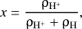
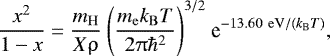
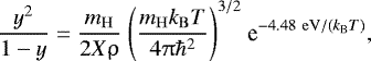
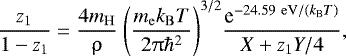
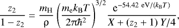
The degree of ionization of atomic hydrogen x, the degree ofdissociation of molecular hydrogen y, and the degrees of single z1 and double z2 ionization ofhelium are defined from D’Angelo & Bodenheimer (2013) as
 (12)
(12)
 (13)
(13)
 (14)
(14)
 (15)
(15)
Following the Boltzmann law of the energy distribution, the ionization and dissociation degrees using Saha equations are given as (see e.g. Black & Bodenheimer 1975)
 (16)
(16)
 (17)
(17)
 (18)
(18)
 (19)
(19)
where me is the electron mass, mH is the hydrogen mass, kB is the Boltzmann constant, ℏ is the Planck’s constant divided by 2π, and ρ = nμmu is the total gas density. The hydrogen and helium mass fractions are taken as X = 0.711 and Y = 0.289, respectively.
For a gas mixture mainly consisting of hydrogen (atoms, molecules, and ions), helium, and a negligible fraction of metals, the mean molecular weight μ is given as (e.g. Black & Bodenheimer 1975)
![Mathematical equation: \begin{align*} {\dfrac{\upmu}{4} = [2X (1 + y + 2xy) + Y (1 + z_1 + z_1 z_2)]^{-1}}, \end{align*}](/articles/aa/full_html/2018/10/aa32635-18/aa32635-18-eq21.png) (20)
(20)
and the gas internal energy density  is given by
 (21)
(21)
The quantity mu is the atomic mass unit and contributions from various species in the parenthesis are dimensionless and can be obtained using an appropriate partition function ζ by taking into account the translational, rotational, and vibrational degrees of freedom as detailed in D’Angelo & Bodenheimer (2013).
The stability condition needed for numerical calculations requires an estimate of the sound speed cs , which relates pressure and density and is defined as
 (22)
(22)
The parameter Γ1 is the first adiabatic index, which has a functional dependence on temperature and density, given as
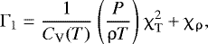 (23)
(23)
where CV(T) is obtained by taking the derivative of the specific gas internal energy e(T) with respect to temperature at a constant volume and the temperature χT and density χρ exponents (see D’Angelo & Bodenheimer 2013) are defined by
 (24)
(24)
 (25)
(25)
We note that for an ideal gas where phase transitions are ignored, i.e. with constant μ and γ , Γ 1 is equal to the adiabatic index γ.
With all of the above considerations, the thermal EOS (relating pressure, temperature, and volume) and the caloric EOS (relating internal energy, volume, and temperature) can be expressed as
 (26)
(26)
where the mean molecular weight μ(X) depends on the gas composition. The chemical fractions are not solved independently and can be expressed as X = X(T, ρ) under equilibrium assumptions. Thus, the thermal and caloric EOS can also be expressed as a function of temperature and density, P = P(ρ, T) and e = e(T, ρ), respectively. Owing to the explicit temperature dependence, the conversion between pressure and internal energy density and vice versa is preceded by computing temperatures using the thermal EOS and pre-computed lookup tables of pressure and internal energy density. Further details on the implementation of lookup tables can be found in Vaidya et al. (2015).
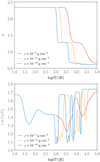 |
Fig. 1 Mean molecular weight μ and adiabatic index γ as a functionof temperature for three different gas densities (ρ = 10−3, 10−11, and 10−19 g cm−3). |
2.2 Opacities
We make use of tabulated dust opacities from Ossenkopf & Henning (1994) and tabulated gas opacities from Malygin et al. (2014). At lower temperatures the contribution from dust dominates, whereas at higher temperatures this is negligible since the dust is evaporated.
Code-wise, we updated the evaporation and sublimation module to consider a time-dependent evolution of the dust. The dust is treated asbeing perfectly coupled to the gas, i.e. the dust is moving with the gas flow, but the dust content is allowed ts1o change in time owing to evaporation and sublimation of dust grains. Hence, we store, in addition to the gas mass density, the local dust-to-gas mass ratio R(t) = Mdust∕Mgas.
The evaporation temperature Tevap is computed based on Pollack et al. (1994) utilizing the power-law formula by Isella & Natta (2005, their Eq. (16)):
 (27)
(27)
where β1 = 2000 K and β2 = 1.95 × 10⁻². In the sublimation regime Tdust < Tevap, the temporal evolution of the dust-to-gas mass ratio R(t) is described by
 (28)
(28)
where dT = |Tevap − Tdust|∕Tevap and d R = (Rmax − R(t))∕Rmax. In the evaporation regime Tdust > Tevap, the temporal evolution of the dust-to-gas mass ratio is described by
 (29)
(29)
The value ω serves as a lower limit to the dR term, which prevents the dR−1 term from diverging.
In a nutshell, evaporation and sublimation become more efficient for higher temperature differences between dust and evaporation temperature. Furthermore, the evaporation efficiency decreases towards lower dust-to-gas mass ratios, and the sublimation efficiency decreases towards the maximum dust-to-gas mass ratio allowed. For all simulations performed, we used Rmax = 0.01, tsubl = 10 yr, tevap = 100 yr, and ω = 0.01.
3 Numerics and initial setup
In this study, 1D spherically symmetric collapse simulations are performed using the (magneto) hydrodynamic code PLUTO (Mignone et al. 2007) combined with the grey FLD radiation transport module MAKEMAKE. The theory and numerics of the radiation transfer scheme are described and tested in Kuiper et al. (2010a, 2018).
Vaytet et al. (2012, 2013) have indicated slight differences in the core properties between grey and multi-group methods. However, they argued that the grey method proves sufficient for the 1D case and the multi-group radiative transfer may be more important in the later evolutionary stages of the protostar. The hydrodynamic equations are solved using a shock capturing Riemann solver within a conservative finite volume scheme, whereas the FLD equation is solved in an implicit way using the generalized minimal residual solver (GMRES). We used the Harten-Lax-VanLeer approximate Riemann solver that restores with the middle contact discontinuity (hllc), a monotonized central difference (MC) flux limiter using piecewise linear interpolation and a Runge–Kutta 2 (RK2) time integration.
As an initial density distribution, we used a stable Bonnor–Ebert (Bonnor 1956; Ebert 1955) sphere like density profile. Comparisons to an initially uniform density cloud are described in Appendix A.
Given an initial cloud mass M0 and outer radius Rout, the initial sound speed cs0 is computed as
 (30)
(30)
where G is the gravitational constant. The initial cloud masses range from 0.5 to 100.0 M⊙ .
The temperature TBE for the stable sphere is calculated as
 (31)
(31)
where μ = 2.353, γ = 5/3, and ℜ is the universal gas constant.
The initial outer ρo and central ρc densities aredetermined by
 (32)
(32)
The density contrast between the centre and edge of the sphere corresponds to a dimensionless radius of ξ = 6.45, where ξ is defined as
 (33)
(33)
where Rcloud is the cloud radius. The integrated mass of the cloud is the same as that of a critical Bonnor–Ebert sphere. The thermal pressure is computed using Eq. (26) for a fixed lower temperature T0 in comparison to the stable Bonnor–Ebert sphere setup, which causes gravity to dominate and initiates the collapse. This temperature T0 varies from 5 to 100 K. The radiation temperature is initially in equilibrium with the gas temperature and the dust and gas temperatures are closely coupled.
For the first set of numerical calculations (see Table 1), the inner radius is fixed to 10−4 au and the outer radius is fixed to 3000 au. This setup implies that the central density of the different Bonnor–Ebert spheres scales as a function of initial cloud mass.
The computational grid for these simulations is comprised of 4416 cells. We used 320 uniformly spaced cells from 10−4 to 10−2 au and 4096 logarithmically spaced cells from 10−2 to 3000 au. We made sure that the last uniform cell and the first logarithmic cell are identical in size. The integration time step in the inner dense core regions becomes very small if a logarithmic binning is used throughout, which would become computationally very expensive. Therefore, we chose a linear grid in the very inner part of the computational domain. We performed convergence tests using different resolutions (see Appendix B.1) and different inner radii Rin (see Appendix B.2) in order to test our approach. These tests show that the applied resolution is fully sufficient and hence there is no need to use higher resolution in the inner parts.
Additionally, in order to investigate the dependence on the initial cloud properties, we explored a range of initial conditions by performing three different set of simulations using a different constant stability parameter MBE∕M0 for the low-mass (0.5–10 M⊙), intermediate-mass (8–20 M⊙) and high-mass regimes (30–100 M⊙), respectively.For these runs, we fixed the outer radius to 3000 au but varied the initial cloud temperature from 5 to 100 K. The initial cloud properties for the selected parameter space are listed in Table 3 and the implications on the first core properties are described in Sect. 4.4. We also perform a set of simulations detailed in Table C.1 with an outer radius of 5000 au and a constant initial temperature of 10 K for initial cloud masses ranging from 1 to 100 M⊙.
At the inner edge Rin we used a reflective boundary condition for the hydrodynamics as well as for radiation transport (no radiative flux should cross the inner boundary interface). At the outer edge Rout, we used a Dirichlet boundary condition on the radiation temperature with a constant boundary value of T0 and an outflow-no-inflow condition for the hydrodynamics that includes a zero-gradient (i.e. no-force) boundary condition for the thermal pressure given as
 (34)
(34)
Initial cloud properties.
4 Results: from clouds to cores
4.1 Fiducial 1 M⊙case
In this section, we present a general overview of the collapse evolution and its effects on various properties for an initial 1 M⊙ cloud. Figure 2 shows the radial profiles of the density, pressure, gas temperature, velocity, enclosed mass, optical depth, Mach number, mean molecular weight μ, and the thermal structure at a time step right after second core formation. We consider an initial Bonnor–Ebert sphere like density profile (as described in Sect. 3), where the initial central density is ρc ≈ 10−17 g cm-3. The evolution of the cloud through its first and second collapse phases can be understood as follows:
Initially the optically thin cloud collapses isothermally with γactual ≈ 1 under its own gravity, where γactual is the change in the slope of the temperature evolution with density (see Fig. 3).
During the first collapse phase, as the density and pressure increases, the optical depth becomes greater than unity (Masunaga & Inutsuka 1999) and the cloud compresses adiabatically. The cloud starts absorbing the thermal radiation and heats up leading to an adiabatic collapse phase.
These conditions lead to the formation of the first hydrostatic core after about 104 yr with initial values of Rfc ≈ 2 au, Mfc ≈10−3M⊙ which subsequently contracts adiabatically with γactual ≈ 5/3.
The strong compression leads to the first shock at the border of the first core as seen in the velocity profile (Fig. 2d). Comparing this to the temperature profile (Fig. 2c), the first shock is supercritical, i.e. pre- and post-shock temperatures are similar as discussed in Commer et al. (2011a).
The first core mainly consists of H2 molecules and neutral He and has a constant mean molecular weight μ of 2.353.
With a rise in temperature, the adiabatic index γ changes from its initial monatomic value γ = 5∕3 to the value for a diatomic gas, γ = 7∕5, once the gas is warm enough to excite the rotational degrees of freedom. As Fig. 3 indicates,γactualundergoes the same evolution.
Once the temperature inside the first core reaches ~2000 K, H2 molecules begin to dissociate, which leads to the second collapse phase. During this phase, γactual changes roughly to 1.1, which is well below the critical value of 4/3 for stability of a self-gravitational sphere.
As the molecular hydrogen and neutral helium concentration changes and the fraction of atomic hydrogen increases duringthe dissociation phase, μ gradually decreases in the inner regions, as seen in Fig. 2h.
Once most of the H2 has been dissociated, it is followed by the formation of the second hydrostatic core with initial values of Rsc ≈ 1.8 × 10⁻² au ≈ 3.9 R⊙, Msc ≈ 4.6 × 10⁻³ M⊙.
-
The second shock at the border of the second core is seen in the velocity profile (Fig. 2d). Comparing this to the temperature profile, the second shock is seen to be subcritical, i.e. the pre-shock temperature being higher than the post-shock temperature, suggesting that the accretion energy is transferred onto the second core and not radiated away.
-
The central density rapidly rises up to ρc ≈ 10−1 g cm-3 at the end of the second collapse phase, which lasts only for a few years since the second hydrostatic core forms almost instantaneously.
At later times when ρc ≈ 10−1 g cm-3, the outer layers tend to have higher temperatures due to the effects of shock heating and absorption of radiation from the hot central region. Differences in the thermal evolution of the central region (black line) and the thermal structure at a timewhen ρc ≈ 10−1 g cm-3 (bluish purple line) can be seen in Fig. 2i.
Finally (not simulated here), once the temperature inside the second core reaches ignition temperatures (≥106 K) for nuclear reactions, it eventually leads to the birth of a star.
Figure 3 summarizes the different evolutionary stages that the molecular cloud undergoes to form the first and second Larson’s cores and indicates the phase transition from monatomic to diatomic gas, i.e. the change in the adiabatic index γ actual.
 |
Fig. 2 Collapse of a 1 M⊙cloud. Radial profiles (across and down) of density (panel a), pressure (panel b), gas temperature (panel c), velocity (panel d), enclosed mass (panel e), optical depth (panel f), Mach number (panel g), mean molecular weight (panel h), and thermal structure (panel i) are shown at the snapshot after second core formation. The black line in panel i shows the temporal evolution of the central temperature and density. The initial profile is shown by the black dot-dashed line, the first collapse phase is indicated by the black dashed line, and the bluish purple line describes the structure after formation of the second hydrostatic core. |
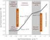 |
Fig. 3 Thermal evolution showing the first and second collapse phases for a 1 M⊙ cloud. The change in adiabatic index γactual indicates the importance of using a realistic gas EOS. |
4.2 Effect of different initial cloud masses
In this section, we discuss the core collapse scenario for different initial cloud masses. We span a wide range of initial cloud masses from 0.5 to 100 M⊙ . The clouds with different initial masses M0 and central densities ρc at the same initial temperature of 10 K and an outer radius of 3000 au follow a similar evolution as seen in Fig. 4. Most significant differences are seen outwards from the first shock as a horizontal spread.
The thermal structure for cases with different initial cloud masses (Fig. 4f) shows that the clouds begin with the same isothermal phase but eventually heat up at different densities. This difference in thermal evolution can have a significant effect on the properties of the first and second cores since for the intermediate- and high-mass clouds (M0 ≥ 8 M⊙ ) the dissociation temperature is reached earlier when the cloud is at a comparatively lower density, which in turn affects the lifetime of the first and second cores. The change in optical depth shown in Fig. 4j as the cloud evolves is mainly governed by the balance between radiative cooling and compressional heating. The sharp dissociation front seen in Fig. 4l indicates that most of the H2 is dissociated at the second core accretion shock.
The first core radius Rfc, defined by the position of the outer discontinuity in the density profile or shock position in velocity profile, is seen to increase with an increase in the initial cloud mass up to around 8–10 M⊙ after which there is a decrease in the first core radius with an increase in the cloud mass (see inset in the radial density profile).
For the initial clouds of mass 40, 60, 80, and 100 M⊙, the first core barely forms and the evolution proceeds rapidly to the second collapse phase. For these cases, since the ram pressure Pram = ρu2 is always higher than the thermal pressure Pgas both above and below the first core radius (see Fig. 4h), gravity acts as a dominant force that prevents a strong first accretion shock. These high-mass clouds also have the highest accretion rate and are the most unstable, which is why they evolve faster. In summary, in the high-mass regime, first cores do not exist.
For comparison with the low- and intermediate-mass regimes, the shock-like velocity structure is still referred to as an “accretion shock” and the first core-like structure is referred to as a “first core” even in the high-mass regime.
The second core radius Rsc is defined by the position of the inner discontinuity in the density profile or inner shock position in the velocity profile. The main properties of the first and second cores for each of the different cases are listed in Table 2. These are the first core mass Mfc , temperature Tfc , and accretion rate Ṁ fc calculated at the first core radius Rfc as well as the second core mass Msc, temperature Tsc, and accretion rate Ṁsc calculated at the second core radius Rsc.
 |
Fig. 4 Shown above are the radial profiles (across and down) of density (panel a), pressure (panel b), gas temperature (panel c), velocity (panel d), and enclosed mass (panel e) as well as the thermal structure (panel f), Mach number (panel g), ratio of gas to ram pressure (panel h), internal energy density as a function of temperature (panel i), optical depth (panel j), Rosseland mean opacity (panel k), and dissociation fraction at the snapshot after second core formation (panel l). Different colours indicate clouds with different initial masses as seen in the colour bar. The grey lines in the thermal structure plot show the 50% dissociation and ionization curves according to Eqs. (16) and (17). |
Properties of the first and second cores estimated at the snapshot after second core formation for different initial cloud masses M0 with a fixed outer radius Rout = 3000 au and initial temperature T0 = 10 K.
4.3 First core properties
In this section we focus on the dependence of the core properties on the initial cloud mass. Our results indicate slight differences (within an order of magnitude) in the first core radius and mass for the collapse simulations with different initial cloud masses. In our studies, since we span a wide range from 0.5 to 100 M⊙, we are able to see a transition region around 8–10 M⊙. Hence, although the differences in the first core properties are within an order of magnitude, we would like to draw more attention to the diminishing first core lifetimes for higher initial cloud masses. This in turn affects the size and mass of the first core.
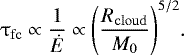
As already noted, the first core radius increases with an increase in the cloud mass until around 8–10 M⊙ after which it decreases. Figure 5a shows the mean first core radius as a function of the initial cloud mass where the mean radius is calculated over time from the onset of the first core formation until the second core formation. The vertical lines span the minimum to maximum first core radius as the core evolves. The transition around 8–10 M⊙ is also seen forthe first core mass (see Fig. 5b), whereas the first core temperature always increases with an increase in the initial cloud mass (see Fig. 5c).
The evolution of the first core radius from the onset of the first core formation until the second core formation is shown in Fig. 6. The first core undergoes an initial contraction phase followed by a rapid expansion and a second contraction phase.
Figure 7 shows the onset of the first core formation as a function of initial cloud mass. In the low-mass range (M0 ≤ 8 M⊙), the cloud is seen to undergo a comparatively slower collapse hence initiating the first core formation after ≈ 5000–18 000 yr. On the other hand, in the intermediate- and high-mass regimes, the collapse is seen to be much faster with the first core forming after a few thousand years (≤5000 yr) followed by an instantaneous second collapse phase that prevents the first core from growing.
Figure 8 shows the first core lifetime as a function of initial cloud mass. The first core lifetime is defined as the time between the onset of formation of the first core until the onset of the second core formation. Since currently we stop our simulations a few years after the second core formation, the total simulation time minus the first core formation time is almost equivalent to that of the first core lifetime.
As seen in all the previous studies, we also note that in the low-mass regime (≤ 8 M⊙ ) the first core lifetime scales as M−0.5 as seen in Fig. 8.
In the intermediate- and high-mass regimes due to the vanishing thermal pressure support, this dependence changes to M−2.5 (see Fig. 8), which can be analytically derived as follows. The accretion energy Ė is given as
 (35)
(35)
where Mfc is the mass enclosed within the first core, Rfc is the first coreradius, τfc is the first core lifetime, and Ṁfc is the accretion rate. The internal energy profiles seen in Fig. 4i look strikingly similar at the onset of the second collapse phase (i.e. at T ≈ 2000 K) for all the different initial cloud masses. This indicates that indeed the internal energy of the first core Efc , at the onset of the second collapse phase, is independent of the initial cloud mass.
Now, we consider the ratio Mfc∕Rfc and multiply and divide by the velocity ufc as follows:
 (36)
(36)
Inserting this into the expression for the accretion energy Ė yields
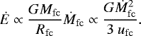 (37)
(37)
In the intermediate- and high-mass regimes, we assume the whole cloud to be in free fall and hence we can relate the local properties to the large scale properties. The accretion rate Ṁ fc is then definedas
 (38)
(38)
where tff is the free fall time. We then assume that the accretion is constant in space (and time), which is valid only for a ρ ∝ R−2 profile, seen in the outer parts of a Bonnor–Ebert sphere like density profile. In this case, the mean velocity ufc can be estimated as
 (39)
(39)
Now, the free-fall time of a collapsing cloud is given by
 (40)
(40)
Using theserelations in the expression for accretion energy Ė , Eq. (37) yields
 (41)
(41)
Furthermore, from Eq. (35)
 (42)
(42)
Thus, in the intermediate- and high-mass regimes, the first core lifetime scales as M−2.5 as seen in Fig. 8. The dependence on the cloud radius is seen in Fig. C.2 and discussed in Appendix C.
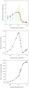 |
Fig. 5 Dependence of the first core properties on initial cloud mass. Panel a: mean first core radius (mean radius is calculated over the time from the onset of the first core formation until the second core formation). The vertical lines span the minimum to maximum first core radius as the core evolves. Panel b: first core mass. Panel c: outer shock temperature as a function of initial cloud mass as estimated at a time after the second core formation when the first core is stable and no longer evolves. A transition region is seen around 8–10 M⊙ indicating the diminishing first core radius and mass towards the high-mass regime. |
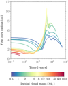 |
Fig. 6 Time evolution of the first core radius showing an initial contraction phase followed by a rapid expansion and a second contraction phase. The colours indicate the different initial cloud masses ranging from 0.5 to 100 M⊙ as shown in the colour bar. |
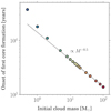 |
Fig. 7 Onsetof formation of the first core for different initial cloud masses. Initially higher mass clouds tend to collapse faster in comparison to the low-mass regime. |
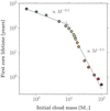 |
Fig. 8 First core lifetime, i.e. time between the onset of formation of the first and second cores for different initial cloud masses. |
4.4 Dependence on initial conditions
In order to assess the robustness of the transition region seen in properties of the first core, we performed three additional set of simulations using a different constant stability parameter MBE∕M0 for the low-mass (0.5–10 M⊙ ), intermediate-mass (8–20 M⊙), and high-mass regimes (30–100 M⊙), respectively, with some overlap between the low and intermediate masses. This implies a change in the initial temperature for the different cases, which now varies from 5 to 100 K. We used three different stability parameters to avoid extremely high initial cloud temperatures in the intermediate- and high-mass regimes. The outer radius for the various simulations is fixed to 3000 au. The different runs with constant stability parameters are listed in Table 3.
We finda transition region in the intermediate-mass regime similar to that described in Sect. 4.3. The mean first core radius increases with an increase in the initial cloud mass until around 5–8 M⊙ and then decreases towards the intermediate- and high-mass regimes. We compare this to the previously described runs with a fixed initial cloud temperature of 10 K in Fig. 9.
Figure 10 shows the dependence of the first core lifetime on the initial cloud mass. It is very similar to that previously seen in Fig. 8, thereby confirming that the first cores are non-existent in the high-mass regime. These results also indicate that the first core properties do not have a very strong dependence on the initial cloud properties.
We also investigated the dependence of the first core properties on the outer cloud radius by performing a set of simulations for the various cases from 1–100 M⊙ using an outer radius of 5000 au. The initial temperature for these runs was kept constant at 10 K. We see a similar transition region in the intermediate-mass regime. The initial cloud properties and first core properties for these runs are described in Appendix C.
Initial cloud properties.
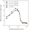 |
Fig. 9 Mean first core radius as a function of initial cloud mass. The mean radius is calculated over the time from the onset of the first core formation until the second core formation. The circles indicate results from the simulation runs with a constant initial temperature of 10 K, whereas the diamonds, triangles, and crosses indicate results from the simulation runs with constant stability parameters MBE ∕M0 of 5.27e-01, 5.27e-02, and 5.27e-03 for the low-, intermediate-, and high-mass regimes, respectively. |
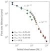 |
Fig. 10 First core lifetime, i.e. time between the onset of formation of the first and second cores for different initial cloud masses. The circles indicate results from the simulation runs with a constant initial temperature of 10 K, whereas the diamonds, triangles, and crosses indicate results from the simulation runs with constant stability parameters MBE ∕M0 of 5.27e-01 , 5.27e-02, and 5.27e-03 for the low-, intermediate-, and high-mass regimes, respectively. |
4.5 Comparison to previous results
In this paper, we expand the collapse simulations for the first time, to cover a wide range of initial cloud masses from 0.5 to 100 M⊙. Figure 11 shows comparisons from our run for an initial 1 M⊙ cloud (bluish purple line) to those by Vaytet & Haugblle (2017; dashed red lines). Both the simulations use an initial Bonnor–Ebert density profile with an outer boundary Rout ≈ 3000 au, ρc ≈ 10−17 g cm-3, and initial temperature of 10 K.
We notethat since the temporal evolution is slightly different in both our studies owing to the differences in the gas EOS (Saumon et al. 1995, used by Vaytet & Haugblle 2017 versus D’Angelo & Bodenheimer 2013 used in this work), opacities, and griding scheme (Lagrangian versus Eulerian), the comparisons are not made at the exact same time but when the central density ρc in both simulations reaches ~10−1 g cm−3.
Vaytet & Haugblle (2017) reported a first core radius of roughly 2 au at the time of formation, which then expands to about 5 au and stays roughly constant for a few hundred years and undergoes a second expansion phase, which increases the core radius to ~8 au. In our simulations, the radius is also roughly 2 au at the time of formation, which then grows to about 5 au and gradually contracts back to ~3 au. Some earlier studies also estimate a first core radius of roughly 3 au, however the core is seen only to be contracting with time (Masunaga et al. 1998; Tomida et al. 2013). The first core lifetime is ~450 yr in comparison to ~415 yr obtained by Vaytet & Haugblle (2017) and ~650 yr by Masunaga & Inutsuka (2000) and Tomida et al. (2013).
For an initial 1 M⊙ cloud, at the end of our simulation, the second core radius is ~3.95 R⊙ in agreement with Masunaga & Inutsuka (2000; ~4 R⊙) and still expanding as seen by Tomida et al. (2013; ~10 R⊙). We note an initial contraction phase followed by expansion due to heating or mass accumulation as also seen by earlier studies (Larson 1969; Masunaga & Inutsuka 2000; Tomida et al. 2013). In comparison, Vaytet & Haugblle (2017) obtained a much smaller second core of roughly 1 R⊙ but they expect the core to expand to larger radii.
We note that Masunaga & Inutsuka (2000) supposed an initial uniform density profile with ρ = 1.415 × 10⁻¹⁹ g cm-3, an outer boundary Rout = 104 au, and initial temperature T0 of 10 K, whereas Tomida et al. (2013) adopted an initial Bonnor–Ebert density profile with ρc = 1.2 × 10⁻¹⁸ g cm-3, an outer boundary Rout ≈ 8800 au, and T0 = 10 K.
Since the studies by Vaytet & Haugblle (2017) are closest to our approach, we further investigated the differences between our results for the collapse of an initial 1 M⊙ cloud using the same temperature-dependent opacities instead of opacity tables (see Appendix D).
All of the previous 1D spherically symmetric radiation hydrodynamic (RHD) studies using frequency-dependent (Masunaga et al. 1998; Masunaga & Inutsuka 2000) and grey FLD approximation (Vaytet & Haugblle 2017) as well as 3D radiation magnetohydrodynamic (RMHD) simulations without rotation and magnetic fields (Tomida et al. 2013) were limited to the low-mass regime (M0 ≤ 10 M⊙). The thermal evolution and properties of the first and second cores from our low-mass runs are in good agreement with these previous works.
In their collapse calculations for the low-mass regime, Vaytet & Haugblle (2017) showed comparisons for different initial cloud masses (M0 ≤ 8 M⊙) at a time after the formation of the second core, which indicates that most significant differences in the radial profiles of different core properties are seen outwards from the first shock as a horizontal spread (see their Fig. 4) that is similar to our results presented in Sect. 4.2.
Baraffe et al. (2012), Vaytet et al. (2013), and Vaytet & Haugblle (2017) found the first core radius and mass to be similar within an order of magnitude for their collapse simulations with different initial cloud masses similar to the results presented herein for the low-mass regime (see Sect. 4.3). Masunaga et al. (1998) noted that the first core radius and mass are independent of the initial cloud mass and density profile, but are weakly dependent on initial cloud temperature and opacity. We also find this weak dependence on initial cloud temperature as discussed in Sect. 4.4.
Tomida et al. (2010a) suggested that the thermal evolution may depend on the initial conditions such as cloud mass, opacities, and temperature. In our studies, since we span a wide range of initial cloud masses beyond 10 M⊙, we find a transition region in the intermediate-mass regime, which indicates a dependence on the initial cloud mass as discussed in Sect. 4.3. We also find a linear dependence of this transition region on the initial cloud radius (see Appendix C).
 |
Fig. 11 Comparisons of our results for an initial 1 M⊙ cloud indicated in bluish purple to those by Vaytet & Haugblle (2017) shown using dashed red line. Radial profiles (across and down) of the density (panel a), pressure (panel b), gas temperature (panel c), velocity (panel d), enclosed mass (panel e), and thermal structure (panel f) are shown at the time when central density ρc in both simulations reach roughly 10−1 g cm-3. |
4.6 Limitations
In our studies, we use spherically symmetric models that neglect the effects of rotation and turbulence. It is however important to take into account effects due to non-negligible internal motions in molecular clouds. Rotation and magnetic fields are expected to have a significant effect on the evolution of the cloud and properties of hydrostatic cores. These effects will be investigated in our future work.
In comparison to pure RHD simulations without rotation, depending on an ideal or a resistive magnetohydrodynamics model and how slow or fast the rotation is, Tomida et al. (2013) found significant differences mostly in the first core lifetime and second core radius (see their Table 2). Tomida et al. (2013) and Vaytet et al. (2013) suggested that the first core lifetime increases slightly in the presence of rotation since it would slow down the collapse.
The lifetimes estimated in our studies can thus be considered as lower limits. Despite the absence of rotation and magnetic fields, our results can still be used as initial conditions in stellar evolution simulations.
5 Summary
We performed 1D radiation hydrodynamic simulations to model the gravitational collapse of a molecular cloud through the formation of the first and second hydrostatic cores. As carried out by some previous studies, we emphasize the importance of using a realistic gas EOS, which takes into account effects such as dissociation, ionization, rotational, and vibrational degrees of freedom for the molecules and which also plays a significant role in accounting for the phase transitions from the monatomic to diatomic gas.
Using an initial constant cloud temperature ranging from 5 to 100 K and an outer radius of 3000 and 5000 au, we model clouds with different initial masses spanning a range from 0.5 to 100 M⊙. For each of these cases, we trace the evolution through an initial isothermal collapse phase, first core formation, adiabatic contraction, H 2 dissociation, second collapse phase, and the second core formation. The thermal evolution of the cloud for the 1 M⊙ cloud is summarized in Fig. 3.
First, we varied the initial cloud mass, keeping a constant initial temperature of 10 K and an outer radius of 3000 au. We note the differences (within an order of magnitude) in the first core properties (listed in Table 2), although the clouds with different initial masses follow a similar evolution. We examine the dependence of the first core properties on the initial cloud mass and find a transition region in the intermediate-mass regime. Our results indicate an increase in the first core radius with an increase in the initial cloud mass until around 8–10 M⊙, after which the first core radius decreases towards the higher initial cloud masses. This trend is also observed when comparing the first core mass for different initial cloud masses.
We would like to draw more attention to the diminishing first core lifetimes for higher initial cloud masses, which in turn affects the size and mass of the first core. It is also highly unlikely to observe first cores with such small lifetimes. Massive clouds have the highest accretion rate and are the most unstable, which is why they evolve faster. For these cases, since the ram pressure is higher than the gas pressure, gravity acts as a dominant force that prevents a strong accretion shock. Hence, we predict that the first cores are non-existent in the high-mass regime.
We confirmed the presence of the transition region in the intermediate-mass regime by performing an additional set of simulations. We use a different constant stability parameter MBE∕M0 for the low-mass (0.5–10 M⊙ ), intermediate-mass (8–20 M⊙), and high-mass regimes (30–100 M⊙), respectively.This implies that the initial cloud temperatures range from 5 to 100 K. The outer cloud radius for these runs is always fixedto 3000 au. We also investigated the influence of the outer cloud radius on the first core properties by performing simulations with a cloud radius of 5000 au for a constant initial temperature of 10 K. We found a similar transition region in the intermediate-mass regime. These results also indicate the weak dependence of the first core properties on the initial cloud temperatureand outer radius.
We note that the results for the first core lifetimes presented in this work should be treated as lower bounds on the core properties since we neglect the effects of rotation and magnetic fields, which could slow down the collapse and in turn affect the core properties. These effects will be taken into account in future studies.
Acknowledgements
We thank the referee for the constructive comments that helped improve this work. A.B. would like to thank Neil Vaytet for useful discussions during this work and for performing dedicated comparison simulations discussed in Appendix D. We would also like to thank Mykola Malygin for providing us with the gas opacity tables. Simulations shown here were run on the Isaac cluster at the Rechenzentrum Garching (RZG) of the Max Planck Society. We further acknowledge computing time on the BinAC cluster from the bwHPC-C5 initiative, funded by the Ministry of Science, Research and the Arts of the State of Baden-Württemberg, Germany. R.K. and A.K. acknowledge financial support via the Emmy Noether Research Group on Accretion Flows and Feedback in Realistic Models of Massive Star Formation funded by the German Research Foundation (DFG) under grant No. KU 2849/3-1. G.D.M. acknowledges support from the Swiss National Science Foundation under grant BSSGI0_155816 “PlanetsInTime” and from the DFG priority programme SPP 1992 “Exploring the Diversity of Extrasolar Planets” (KU 2849/7-1). Parts of this work have been carried out within the frame of the National Centre for Competence in Research PlanetS supported by the SNSF. The authors acknowledge support by the High Performance and Cloud Computing Group at the Zentrum fr Datenverarbeitung of the University of Tübingen, the State of Baden-Württemberg through bwHPC, and the German Research Foundation (DFG) through grant No. INST 37/935-1 FUGG.
Appendix A Comparisons to a uniform density cloud
There have been previous collapse studies using a uniform density cloud as an initial setup instead of the Bonnor–Ebert sphere as considered in this work. However, the uniform density cloud eventually evolves into a Bonnor–Ebert-like profile (Larson 1969; Masunaga et al. 1998). We compare the effect of a uniform density and Bonnor–Ebert-like density profile on the core properties. Figure A.1 shows the radial profiles of the density and velocity and the ratio of gas to ram pressure for collapse of a 1 M⊙ cloud for three different cases, using an initial Bonnor–Ebert sphere at 10 K (blue) and a uniform cloud at 10 K (dashed red) and 30 K (dashed yellow).
For the 30 K uniform density cloud and the 10 K Bonnor–Ebert sphere clouds, we note that the initial density profile does not have a significant effect on evolution of the cloud as also seen by Vaytet & Haugblle (2017). However, in comparison to the Bonnor–Ebert sphere setup, the evolution of a uniform density cloud is much slower (~ 3 × 10⁴ yr). In contrast, Masunaga & Inutsuka (2000) argued that the initial density profile does affect the protostellar evolution due to different dynamics. Since there are no significant differences between the two density profiles, in our studies we used a Bonnor–Ebert sphere as an initial density profile. Vaytet & Haugblle (2017) also suggested that a Bonnor–Ebert sphere is a better representation of the collapsing cloud.
In case of a 10 K uniform density cloud, we note a different behaviour. In this case, the strong ram pressure due to the high infall velocities is always higher than the gas pressure as seen in Fig. A.1. This may be because the clouds are highly unstable and gravity acts as the dominant force and there is little effect due to pressure forces, which prevents the formation of the first hydrostatic core. A similar case devoid of the first accretion shock is seen by Vaytet & Haugblle (2017). They used an initial uniform density setup for a 4 M⊙ cloud collapse at an initial temperature of 5 K. This behaviour of the 10 K uniform density cloud does not invalidate the previousstudies that used initial uniform density, since the clouds were not unstable to skip the first core formation.
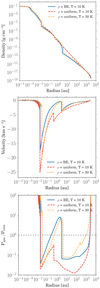 |
Fig. A.1 Radial profiles of the density, velocity, and the ratio of gas to ram pressure for collapse of a 1 M⊙ cloud for three different cases, using an initial Bonnor–Ebert sphere (blue) at 10 K, uniform cloud at 10 K (dashed red), and uniform cloud at 30 K (dashed yellow) are shown at a time step after the second core formation. |
Appendix B Numerical convergence
B.1 Resolution tests
Resolution plays an important role especially when treating regions near accretion shocks. For an initial 1 M⊙ cloud, we performed core collapse simulations with the exact same initial conditions but using different resolutions. The simulations using different resolutions have no significant effects on the evolution seen in Fig. B.1, which indicates the numerically convergence for our studies. As expected for the lowest resolution, owing to fewer grid cells in the inner region, we see slight differences at the second shock position. These differences probably increase for even lower resolutions. There seems to be a convergence around 4400 cells and above. This indicates a minimum resolution of around 4400 cells required for our simulations.
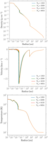 |
Fig. B.1 Radial profiles of the density, velocity, and gas temperature for an initial 1 M⊙ cloud at an initial temperature T0 of 10 K are shown at a time step after the second core formation. The different lines indicate the results using various grid resolutions. |
B.2 Comparisons for different inner radii
In order to ensure that the inner radius does not affect the second shock position, we ran some tests with different inner radii. As seen in Fig. B.2, all of the runs evolve in a similar manner. We note the differences for the simulations with Rin = 3 × 10⁻⁴ au and Rin = 10−3 au. However, there seems to be a convergence for an inner radius around 10−4 au. For our studies, we chose an inner radius of 10−4 au to avoid the boundary being too close to the second shock.
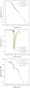 |
Fig. B.2 Radial profiles of the density, velocity, and gas temperature for an initial 1 M⊙ cloud are shown at a time step after the second core formation. The different lines indicate the results each using a different inner radius of the cloud. The dashed blue line indicates 10−5 au, the red line indicates 10−4 au, the dashed green line indicates 3 × 10⁻⁴ au, and the dashed yellow line indicates 10−3 au. |
Appendix C Dependence on initial cloud radius
In order to test the robustness of the transition region seen in the first core properties as described in our results, we performed an additional set of simulations spanning initial cloud masses from 1–100 M⊙ at a constant initial temperature of 10 K, but with a larger outer radius Rout of 5000 au. The computational grid for these simulations comprises of 4568 cells. We use 320 uniformly spaced cells from 10−4 to 10−2 au and 4248 logarithmically spaced cells from 10−2 to 5000 au. We again made sure that the last uniform cell and the first logarithmic cell are identical in size as described previously in Sect. 3.
Figure C.1 shows an increase in the mean first core radius until around 12–14 M⊙ beyond which it decreases towards the high-mass regime. Figure C.2 indicates a shorter first core lifetime towards intermediate- and high-mass regimes. In this figure, we compare the mean first core radius and first core lifetime from the runs with an outer radius of 3000 au (shown as circles) to those with an outer radius of 5000 au (shown as diamonds). We see that the lifetime scales as M−2.5 in the intermediate- and high-mass regimes. In this case, the fit (dashed line) also incorporates the radial dependence of R−2.5 as derived in Sect. 4.3.
Initial cloud properties.
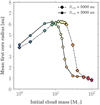 |
Fig. C.1 Mean first core radius as a function of initial cloud mass. The mean radius is calculated over the time from the onset of the first core formation until the second core formation. Comparisons from two different set of simulations with an outer cloud radius of 3000 au (circles) and 5000 au (diamonds) are shown. |
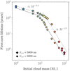 |
Fig. C.2 First core lifetime, i.e. time between the onset of formation of the first and second cores for different initial cloud masses. Comparisons from two different set of simulations with an outer cloud radius of 3000 au (circles) and 5000 au (diamonds) are shown. |
We thusconfirm the presence of a transition region in the intermediate-mass regime seen in the first core radius and lifetime, which indicates that first cores are non-existent in the high-mass regime. We find a linear dependence of the transition mass on the initial cloud radius.
Appendix D Effect of opacities
We present comparison studies between our simulations and those kindly provided by N. Vaytet (2017, priv. comm.) mainly focussing onthe effect of opacities.
As described in Sect. 4.5, since the studies by Vaytet & Haugblle (2017) are closest to our approach we compared our results for the collapse of a 1 M⊙ cloud at an initial temperature of 10 K. We note the discrepancies owing to the differences in the gas EOS (Saumon et al. 1995 used by Vaytet & Haugblle 2017 versus D’Angelo & Bodenheimer 2013 used in this work), opacity tables, and griding scheme (Lagrangianversus Eulerian) as seen in Fig. 11.
In order to investigate the effect of opacities, we compared our simulation for the collapse of a 1 M⊙ cloud using a temperature-dependent opacity  to the simulation provided by N. Vaytet (2017, priv. comm.) performed for an identical initial setup using the same temperature-dependent opacity. In both these runs, T0 = 10 K. As seen in Fig. D.1, although his simulations (dashed red line) still tend to produce a bigger first core radius, the difference is smaller compared to using different opacity tables (see Fig. 11). The second core does not contract as much in our simulations (bluish purple line), however as predicted the second core in his simulation may expand to obtain a value close to ours. These comparisons indicate that opacities play a role in determining the core properties but only provide some fine-tuning. Thus, the main properties derived herein are still robust.
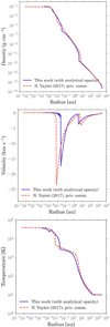 |
Fig. D.1 Radial profiles of the density, velocity, and gas temperature of an initial 1 M⊙ cloud at an initial temperature T0 of 10 K are shown at the time when central density ρc in both simulations reach roughly 10−1 g cm-3. The bluish purple solid lines show results from simulations described in Sect. 3, while the dashed red line represents results from simulations provided by N. Vaytet (2017, priv. comm.). We note that for this comparison both codes use the same temperature-dependent opacity |
In addition, the different treatment of the gas EOS and griding scheme may also contribute to the differences. We note that since the temporal evolution is slightly different in both our studies owing to these differences, the comparisons are not made at the exact same time but when the central density ρc in both simulations reaches ~10−1 g cm-3.
References
- Baraffe, I., Vorobyov, E., & Chabrier, G. 2012, ApJ, 756, 118 [NASA ADS] [CrossRef] [Google Scholar]
- Bate, M. R., Tricco, T. S., & Price, D. J. 2014, MNRAS, 437, 77 [NASA ADS] [CrossRef] [Google Scholar]
- Black, D. C., & Bodenheimer, P. 1975, ApJ, 199, 619 [NASA ADS] [CrossRef] [Google Scholar]
- Bodenheimer, P., & Sweigart, A. 1968, ApJ, 152, 515 [NASA ADS] [CrossRef] [Google Scholar]
- Bonnor, W. B. 1956, MNRAS, 116, 351 [CrossRef] [Google Scholar]
- Commer, B., Audit, E., Chabrier, G., & Chi, J.-P. 2011a, A&A, 530, A13 [NASA ADS] [CrossRef] [EDP Sciences] [Google Scholar]
- Commer, B., Teyssier, R., Audit, E., Hennebelle, P., & Chabrier, G. 2011b, A&A, 529, A35 [NASA ADS] [CrossRef] [EDP Sciences] [Google Scholar]
- D’Angelo, G., & Bodenheimer, P. 2013, ApJ, 778, 77 [NASA ADS] [CrossRef] [Google Scholar]
- Dunham, M. M., Stutz, A. M., Allen, L. E., et al. 2014, Protostars and Planets VI, 195 [Google Scholar]
- Ebert, R. 1955, Z. Astrophys., 37, 217 [NASA ADS] [Google Scholar]
- Inutsuka, S.-i. 2012, Prog. Theor. Exp. Phys., 2012, 01A307 [Google Scholar]
- Isella, A., & Natta, A. 2005, A&A, 438, 899 [NASA ADS] [CrossRef] [EDP Sciences] [Google Scholar]
- Kuiper, R., Klahr, H., Dullemond, C., Kley, W., & Henning, T. 2010a, A&A, 511, A81 [NASA ADS] [CrossRef] [EDP Sciences] [Google Scholar]
- Kuiper, R., Klahr, H., Beuther, H., & Henning, T. 2010b, ApJ, 722, 1556 [CrossRef] [Google Scholar]
- Kuiper, R., Klahr, H., Beuther, H., & Henning, T. 2011, ApJ, 732, 20 [NASA ADS] [CrossRef] [Google Scholar]
- Kuiper, R., Yorke, H. W., & Mignone, A. 2018, A&A, submitted [Google Scholar]
- Larson, R. B. 1969, MNRAS, 145, 271 [NASA ADS] [CrossRef] [Google Scholar]
- Larson, R. B. 2003, Rep. Prog. Phys., 66, 1651 [NASA ADS] [CrossRef] [Google Scholar]
- Launhardt, R., Stutz, A. M., Schmiedeke, A., et al. 2013, A&A, 551, A98 [NASA ADS] [CrossRef] [EDP Sciences] [Google Scholar]
- Levermore, C. D., & Pomraning, G. C. 1981, ApJ, 248, 321 [NASA ADS] [CrossRef] [Google Scholar]
- Malygin, M. G., Kuiper, R., Klahr, H., Dullemond, C. P., & Henning, T. 2014, A&A, 568, A91 [NASA ADS] [CrossRef] [EDP Sciences] [Google Scholar]
- Masunaga, H., & Inutsuka, S.-i. 1999, ApJ, 510, 822 [NASA ADS] [CrossRef] [Google Scholar]
- Masunaga, H., & Inutsuka, S.-i. 2000, ApJ, 531, 350 [NASA ADS] [CrossRef] [Google Scholar]
- Masunaga, H., Miyama, S. M., & Inutsuka, S.-i. 1998, ApJ, 495, 346 [Google Scholar]
- McKee, C. F., & Ostriker, E. C. 2007, ARA&A, 45, 565 [NASA ADS] [CrossRef] [Google Scholar]
- Mignone, A., Bodo, G., Massaglia, S., et al. 2007, ApJS, 170, 228 [Google Scholar]
- Mignone, A., Zanni, C., Tzeferacos, P., et al. 2012, ApJS, 198, 7 [Google Scholar]
- Nakano, T. 1998, ApJ, 494, 587 [NASA ADS] [CrossRef] [Google Scholar]
- Nielbock, M., Launhardt, R., Steinacker, J., et al. 2012, A&A, 547, A11 [NASA ADS] [CrossRef] [EDP Sciences] [Google Scholar]
- Ossenkopf, V., & Henning, T. 1994, A&A, 291, 943 [NASA ADS] [Google Scholar]
- Pollack, J. B., Hollenbach, D., Beckwith, S., et al. 1994, ApJ, 421, 615 [NASA ADS] [CrossRef] [Google Scholar]
- Saumon, D., Chabrier, G., & van Horn, H. M. 1995, ApJS, 99, 713 [NASA ADS] [CrossRef] [Google Scholar]
- Shu, F. H., Adams, F. C., & Lizano, S. 1987, ARA&A, 25, 23 [Google Scholar]
- Stahler, S. W., Shu, F. H., & Taam, R. E. 1980a, ApJ, 241, 637 [NASA ADS] [CrossRef] [Google Scholar]
- Stahler, S. W., Shu, F. H., & Taam, R. E. 1980b, ApJ, 242, 226 [NASA ADS] [CrossRef] [Google Scholar]
- Stahler, S. W., Shu, F. H., & Taam, R. E. 1981, ApJ, 248, 727 [NASA ADS] [CrossRef] [Google Scholar]
- Stamatellos, D., & Whitworth, A. P. 2009, MNRAS, 400, 1563 [NASA ADS] [CrossRef] [Google Scholar]
- Stamatellos, D., Whitworth, A. P., Bisbas, T., & Goodwin, S. 2007, A&A, 475, 37 [NASA ADS] [CrossRef] [EDP Sciences] [Google Scholar]
- Tomida, K., Machida, M. N., Saigo, K., Tomisaka, K., & Matsumoto, T. 2010a, ApJ, 725, L239 [NASA ADS] [CrossRef] [Google Scholar]
- Tomida, K., Machida, M. N., Saigo, K., Tomisaka, K., & Matsumoto, T. 2010b, ApJ, 714, L58 [NASA ADS] [CrossRef] [Google Scholar]
- Tomida, K., Tomisaka, K., Matsumoto, T., et al. 2013, ApJ, 763, 6 [NASA ADS] [CrossRef] [Google Scholar]
- Vaidya, B., Mignone, A., Bodo, G., & Massaglia, S. 2015, A&A, 580, A110 [NASA ADS] [CrossRef] [EDP Sciences] [Google Scholar]
- Vaytet, N., & Haugblle, T. 2017, A&A, 598, A116 [NASA ADS] [CrossRef] [EDP Sciences] [Google Scholar]
- Vaytet, N., Audit, E., Chabrier, G., Commer, B., & Masson, J. 2012, A&A, 543, A60 [NASA ADS] [CrossRef] [EDP Sciences] [Google Scholar]
- Vaytet, N., Chabrier, G., Audit, E., et al. 2013, A&A, 557, A90 [NASA ADS] [CrossRef] [EDP Sciences] [Google Scholar]
- Vaytet, N., Tomida, K., & Chabrier, G. 2014, A&A, 563, A85 [NASA ADS] [CrossRef] [EDP Sciences] [Google Scholar]
- Whitehouse, S. C., & Bate, M. R. 2006, MNRAS, 367, 32 [NASA ADS] [CrossRef] [Google Scholar]
- Winkler, K.-H. A., & Newman, M. J. 1980a, ApJ, 236, 201 [NASA ADS] [CrossRef] [Google Scholar]
- Winkler, K.-H. A., & Newman, M. J. 1980b, ApJ,238, 311 [NASA ADS] [CrossRef] [Google Scholar]
All Tables
Properties of the first and second cores estimated at the snapshot after second core formation for different initial cloud masses M0 with a fixed outer radius Rout = 3000 au and initial temperature T0 = 10 K.
All Figures
|
Fig. 1 Mean molecular weight μ and adiabatic index γ as a functionof temperature for three different gas densities (ρ = 10−3, 10−11, and 10−19 g cm−3). |
| In the text | |
|
Fig. 2 Collapse of a 1 M⊙cloud. Radial profiles (across and down) of density (panel a), pressure (panel b), gas temperature (panel c), velocity (panel d), enclosed mass (panel e), optical depth (panel f), Mach number (panel g), mean molecular weight (panel h), and thermal structure (panel i) are shown at the snapshot after second core formation. The black line in panel i shows the temporal evolution of the central temperature and density. The initial profile is shown by the black dot-dashed line, the first collapse phase is indicated by the black dashed line, and the bluish purple line describes the structure after formation of the second hydrostatic core. |
| In the text | |
|
Fig. 3 Thermal evolution showing the first and second collapse phases for a 1 M⊙ cloud. The change in adiabatic index γactual indicates the importance of using a realistic gas EOS. |
| In the text | |
|
Fig. 4 Shown above are the radial profiles (across and down) of density (panel a), pressure (panel b), gas temperature (panel c), velocity (panel d), and enclosed mass (panel e) as well as the thermal structure (panel f), Mach number (panel g), ratio of gas to ram pressure (panel h), internal energy density as a function of temperature (panel i), optical depth (panel j), Rosseland mean opacity (panel k), and dissociation fraction at the snapshot after second core formation (panel l). Different colours indicate clouds with different initial masses as seen in the colour bar. The grey lines in the thermal structure plot show the 50% dissociation and ionization curves according to Eqs. (16) and (17). |
| In the text | |
|
Fig. 5 Dependence of the first core properties on initial cloud mass. Panel a: mean first core radius (mean radius is calculated over the time from the onset of the first core formation until the second core formation). The vertical lines span the minimum to maximum first core radius as the core evolves. Panel b: first core mass. Panel c: outer shock temperature as a function of initial cloud mass as estimated at a time after the second core formation when the first core is stable and no longer evolves. A transition region is seen around 8–10 M⊙ indicating the diminishing first core radius and mass towards the high-mass regime. |
| In the text | |
|
Fig. 6 Time evolution of the first core radius showing an initial contraction phase followed by a rapid expansion and a second contraction phase. The colours indicate the different initial cloud masses ranging from 0.5 to 100 M⊙ as shown in the colour bar. |
| In the text | |
|
Fig. 7 Onsetof formation of the first core for different initial cloud masses. Initially higher mass clouds tend to collapse faster in comparison to the low-mass regime. |
| In the text | |
|
Fig. 8 First core lifetime, i.e. time between the onset of formation of the first and second cores for different initial cloud masses. |
| In the text | |
|
Fig. 9 Mean first core radius as a function of initial cloud mass. The mean radius is calculated over the time from the onset of the first core formation until the second core formation. The circles indicate results from the simulation runs with a constant initial temperature of 10 K, whereas the diamonds, triangles, and crosses indicate results from the simulation runs with constant stability parameters MBE ∕M0 of 5.27e-01, 5.27e-02, and 5.27e-03 for the low-, intermediate-, and high-mass regimes, respectively. |
| In the text | |
|
Fig. 10 First core lifetime, i.e. time between the onset of formation of the first and second cores for different initial cloud masses. The circles indicate results from the simulation runs with a constant initial temperature of 10 K, whereas the diamonds, triangles, and crosses indicate results from the simulation runs with constant stability parameters MBE ∕M0 of 5.27e-01 , 5.27e-02, and 5.27e-03 for the low-, intermediate-, and high-mass regimes, respectively. |
| In the text | |
|
Fig. 11 Comparisons of our results for an initial 1 M⊙ cloud indicated in bluish purple to those by Vaytet & Haugblle (2017) shown using dashed red line. Radial profiles (across and down) of the density (panel a), pressure (panel b), gas temperature (panel c), velocity (panel d), enclosed mass (panel e), and thermal structure (panel f) are shown at the time when central density ρc in both simulations reach roughly 10−1 g cm-3. |
| In the text | |
|
Fig. A.1 Radial profiles of the density, velocity, and the ratio of gas to ram pressure for collapse of a 1 M⊙ cloud for three different cases, using an initial Bonnor–Ebert sphere (blue) at 10 K, uniform cloud at 10 K (dashed red), and uniform cloud at 30 K (dashed yellow) are shown at a time step after the second core formation. |
| In the text | |
|
Fig. B.1 Radial profiles of the density, velocity, and gas temperature for an initial 1 M⊙ cloud at an initial temperature T0 of 10 K are shown at a time step after the second core formation. The different lines indicate the results using various grid resolutions. |
| In the text | |
|
Fig. B.2 Radial profiles of the density, velocity, and gas temperature for an initial 1 M⊙ cloud are shown at a time step after the second core formation. The different lines indicate the results each using a different inner radius of the cloud. The dashed blue line indicates 10−5 au, the red line indicates 10−4 au, the dashed green line indicates 3 × 10⁻⁴ au, and the dashed yellow line indicates 10−3 au. |
| In the text | |
|
Fig. C.1 Mean first core radius as a function of initial cloud mass. The mean radius is calculated over the time from the onset of the first core formation until the second core formation. Comparisons from two different set of simulations with an outer cloud radius of 3000 au (circles) and 5000 au (diamonds) are shown. |
| In the text | |
|
Fig. C.2 First core lifetime, i.e. time between the onset of formation of the first and second cores for different initial cloud masses. Comparisons from two different set of simulations with an outer cloud radius of 3000 au (circles) and 5000 au (diamonds) are shown. |
| In the text | |
|
Fig. D.1 Radial profiles of the density, velocity, and gas temperature of an initial 1 M⊙ cloud at an initial temperature T0 of 10 K are shown at the time when central density ρc in both simulations reach roughly 10−1 g cm-3. The bluish purple solid lines show results from simulations described in Sect. 3, while the dashed red line represents results from simulations provided by N. Vaytet (2017, priv. comm.). We note that for this comparison both codes use the same temperature-dependent opacity |
| In the text | |
Current usage metrics show cumulative count of Article Views (full-text article views including HTML views, PDF and ePub downloads, according to the available data) and Abstracts Views on Vision4Press platform.
Data correspond to usage on the plateform after 2015. The current usage metrics is available 48-96 hours after online publication and is updated daily on week days.
Initial download of the metrics may take a while.