| Issue |
A&A
Volume 616, August 2018
|
|
|---|---|---|
| Article Number | A78 | |
| Number of page(s) | 30 | |
| Section | Interstellar and circumstellar matter | |
| DOI | https://doi.org/10.1051/0004-6361/201731778 | |
| Published online | 22 August 2018 | |
Structure and fragmentation of a high line-mass filament: Nessie⋆
1
Max-Planck-Institut für Radioastronomie, Auf dem Hügel 69, 53121 Bonn, Germany
e-mail mmattern@mpifr-bonn.mpg.de
2
Max-Planck-Institut für Astronomie, Königstuhl 17, 69117 Heidelberg, Germany
3
Department of Space, Earth and Environment, Chalmers University of Technology, Onsala Space Observatory, 439 92 Onsala, Sweden
Received:
15
August
2017
Accepted:
29
March
2018
Context. An increasing number of hundred-parsec-scale, high line-mass filaments are being detected in the Galaxy. Their evolutionary path, including fragmentation towards star formation, is virtually unknown.
Aims. We characterize the fragmentation within the hundred-parsec-scale, high line-mass Nessie filament, covering size-scales in the range ~0.1–100 pc. We also connect the small-scale fragments to the star-forming potential of the cloud.
Methods. We combine near-infrared data from the VISTA Variables in the Via Lactea (VVV) survey with mid-infrared Spitzer/GLIMPSE data to derive a high-resolution dust extinction map for Nessie. We then apply a wavelet decomposition technique on the map to analyze the fragmentation characteristics of the cloud. The characteristics are then compared with predictions from gravitational fragmentation models. We compare the detected objects to those identified at a resolution approximately ten times lower from ATLASGAL 870 μm dust emission data.
Results. We present a high-resolution extinction map of Nessie (2″ full-width-half-max, FWHM, corresponding to 0.03 pc). We estimate the mean line mass of Nessie to be ~627 M⊙ pc−1 and the distance to be ~3.5 kpc. We find that Nessie shows fragmentation at multiple size scales. The median nearest-neighbor separations of the fragments at all scales are within a factor of two of the Jeans’ length at that scale. However, the relationship between the mean densities of the fragments and their separations is significantly shallower than expected for Jeans’ fragmentation. The relationship is similar to the one predicted for a filament that exhibits a Larson-like scaling between size-scale and velocity dispersion; such a scaling may result from turbulent support. Based on the number of young stellar objects (YSOs) in the cloud, we estimate that the star formation rate (SFR) of Nessie is ~371 M⊙ Myr−1; similar values result if using the number of dense cores, or the amount of dense gas, as the proxy of star formation. The star formation efficiency is 0.017. These numbers indicate that by its star-forming content, Nessie is comparable to the Solar neighborhood giant molecular clouds like Orion A.
Key words: stars: formation / infrared: ISM / ISM: clouds / dust, extinction
The extinction map (Fig. 5, FITS file) is only available at the CDS via anonymous ftp to cdsarc.u-strasbg.fr (130.79.128.5) or via http://cdsarc.u-strasbg.fr/viz-bin/qcat?J/A+A/616/A78
© ESO 2018
1. Introduction
Star formation is an important process in the evolution of galaxies and the Universe. It plays a crucial role in gas-to-stars conversion through parameters such as star-forming rate (SFR) and star-formation efficiency (SFE), and the initial mass function (e.g., McKee & Ostriker 2007; Hennebelle & Falgarone 2012; Padoan et al. 2014). Star formation takes place in dense regions of molecular clouds, which appear to be commonly composed of filamentary structures (Schneider & Elmegreen 1979; Arzoumanian et al. 2011; Hacar et al. 2013; Schisano et al. 2014; Li et al. 2016; Kainulainen et al. 2017; Stutz & Gould 2016, see André et al. 2014 for a review). Filaments are observationally defined as any elongated structures with an aspect ratio larger than approximately five and a clearly higher density than their surroundings (Myers 2009). Given the link between filamentary structures and star formation, the processes driving the formation and evolution of filaments are linked with SFR and SFE. However, these processes are still not well understood.
Specifically, the physics of filament fragmentation is not well known. This is mostly because determining the basic characteristics of filaments is observationally challenging, as the cold molecular hydrogen is invisible to observations. Therefore, different tracers and techniques are needed to determine its distribution and properties (e.g., Lombardi & Alves 2001; Goldsmith et al. 2008; Goodman et al. 2009; André et al. 2014). Each of the techniques is sensitive to different density regimes and has different spatial resolution. For studies of the structures related to star formation, the resolution should clearly resolve the Jeans’ length. This is about 0.1 pc for typical conditions of a molecular cloud (gas temperature T = 15 K, average density n̄(H) = 105 cm−3). This currently limits the observations to mostly nearby (<500 pc) clouds. Interferometric observations can increase this resolution further, but they have their own caveats (e.g., spatial filtering, slow mapping speed).
However, the nearby clouds that can be systematically mapped in high-enough resolution are mainly low-mass clouds, containing mostly low line-mass filaments (mass per unit length of (M/l) ≲ a few ×10 M⊙) forming almost exclusively low-mass stars. An exception to this is the integral shaped filament in the Orion A cloud (at distance 414 pc, Menten et al. 2007) whose fragmentation has been analyzed in high resolution using interferometric data (e.g., Takahashi et al. 2013; Teixeira et al. 2016; Kainulainen et al. 2017). In general, however, our current observational picture of filaments is mostly built by data on low-mass clouds. Filaments that have much higher line masses ((M/l) ≫ 100 M⊙), and may also be able to form high-mass stars, have been identified in numbers, but they are typically located at farther distances (e.g., Jackson et al. 2010; Hernandez et al. 2012; Busquet et al. 2013; Kainulainen et al. 2013; Ragan et al. 2014; Wang et al. 2014, 2016; Beuther et al. 2015; Abreu-Vicente et al. 2016; Henshaw et al. 2016; Li et al. 2016). Modern facilities are only just approaching the ability to study them systematically at a resolution that resolves the Jeans’ scale.
Recently, Kainulainen & Tan (2013) developed a dust-extinction-based method that allows studying infrared dark molecular clouds at a resolution of ~2″ over a wide dynamic range of column densities, using a combination of near- and mid-infrared observations (see also Lombardi & Alves 2001; Kainulainen et al. 2011; Butler & Tan 2012). This method allows us to analyze the internal structure of clouds up to several kpc distance at ~0.1 pc resolution, enabling fragmentation studies of high line-mass filaments.
With the high-resolution mapping technique in hand, we can address a basic question related to filament fragmentation: What are the fragmentation characteristics of massive filaments and are they in agreement with gravitational fragmentation models?
In this paper, we take advantage of the high resolution provided by the Kainulainen & Tan (2013) extinction-mapping technique and analyze the fragmentation characteristics of a ~100 pc-long, high line-mass filamentary cloud known as “Nessie” (Jackson et al. 2010). It is supposedly located within the Scutum-Centaurus Arm of the Milky Way (Goodman et al. 2014; Ragan et al. 2014; Zucker et al. 2015; Abreu-Vicente et al. 2016). The high resolution allows us to characterize the cloud structure and to gauge the fragmentation processes over a wide range of scales (~0.1–100 pc). We use the dust extinction mapping technique in conjunction with the near-infrared (NIR) data from the ESO/VISTA telescope and mid-infrared (MIR) data from the Spitzer satellite. We subsequently analyze the derived column density map with a hierarchical structure-identification technique and examine the fragmentation of the cloud over multiple size-scales. The results are then compared with theoretical models and other clouds in the literature. Finally, we compare our identified small-scale structures to clumps identified in low-resolution (~20″) dust emission maps by Csengeri et al. (2014). This demonstrates how structures identified from data with ten times lower resolution are seen to fragment when viewed in finer detail.
2. Data
2.1. Infrared data and data reduction
We employ NIR imaging data from the VISTA Variables in the Via Lactea (VVV) survey (Saito et al. 2012) at the 4.1 m VISTA telescope of the Paranal Observatory. The calibrated and reduced data are publicly available in the ESO archive. Specifically, we used the J, H, KS spectral bands of the tiles d069 and d068. For each filter band there are two texp = 80 s exposures and additionally there are 8 and 12 texp = 16 s exposures of tiles d069 and d068 in the KS band, respectively. The pixel size of the images is 0.34″ × 0.34″. Detailed information about the observations can be found in Table A.1 in the appendix. We stacked the observations and performed point-spread-function (PSF) photometry with the daophot package (Stetson 1987) using the Image Reduction and Analysis Facility (IRAF) software. The PSF model was created from bright isolated stars with the model radius of rPSF = 1.5″. The different spatial resolutions of the single-observation epochs has no significant effect on the photometry as we show in Appendix B. The daophot algorithm identifies and extracts extended sources and cosmic rays, and we expect only a very low contamination of the data by galaxies because we are looking through the galactic mid-plane. The zero-point magnitudes were defined by comparing the resulting magnitudes of the stars with the corresponding stars of 2MASS, that are flagged as good photometric quality (Cutri et al. 2003; Skrutskie et al. 2006). This resulted in zero-points Jzpt = 21, 21 mag, Hzpt = 21, 22 mag, and KS,zpt = 20, 88 mag. The resulting data show the expected shape in the NIR color-color scatter plot (Fig. 1), with a bump for the main sequence stars and an elongated distribution for stars with varying reddening. We also tested the photometry measurements for completeness by adding artificial stars. We could identify all artificial stars up to a magnitude of about Jcom = 16.5 mag, Hcom = 15.5 mag, and KS,com = 15.0 mag.
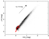 |
Fig. 1. NIR color-color diagram of all sources in the mapped area extracted from the VVV survey with the photometric errors lower than 0.02 mag. The blue crosses indicate non-reddened intrinsic colors of stars (Bessell & Brett 1998). The arrow shows the reddening for an extinction of AV = 10 mag. |
We also employ MIR 8 μm imaging data from the Spitzer/GLIMPSE survey, data release 5 (Benjamin et al. 2003; Churchwell et al. 2009). The pipeline-reduced (S13.2.0 1v04) images were retrieved from the IRSA1 database and used as such. The 8 μm image has a spatial resolution of 2.4″ and a pixel size of 1.2″ times 1.2″. The used tile is centered around RA = 16:43:14.08, Dec = −16:00:15.92. The effective integration time of the tile is 1.2 s.
2.2. ATLASGAL data
We also use data from the APEX telescope large area survey of the galaxy (ATLASGAL, Schuller et al. 2009) for a comparison with our extinction data. The survey was obtained by the Millimeter and Submillimeter Group of the Max-Planck-Institut für Radioastronomie from 2007 to 2010 at the Atacama Pathfinder Experiment (APEX) located on Chajnantor in Chile. The survey instrument was the Large APEX Bolometer Camera (LABOCA) observing at 870 μm, which traces the thermal dust emission. The resolution of the survey is Ω = 19.2″ with a sensitivity in the range of 40–70 mJy/beam. The maps covering the Nessie filament are centered at l = −22.5°, b = 0.0° and l = −19.5°, b = 0.0° and were observed on August 18 and 21 of 2007. The flux per beam, Fν of the ATLASGAL map can be used to estimate the hydrogen column density N(H2) under the assumptions of a constant gas-to-dust ratio of R = 100 and a dust opacity of κ345 GHz = 1.85 cm2 g−1, which was extrapolated by Schuller et al. (2009) based on the work of Ossenkopf & Henning (1994),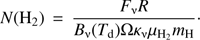 (1)
(1)
Bν(Td) is the Planck function at the dust temperature Td, mH is the mass of a hydrogen atom, and μH2 the mean molecular weight of the interstellar medium with respect to hydrogen molecules, which is 2.8 (Kauffmann et al. 2008).
Csengeri et al. (2014) have identified clump-like structures from the ATLASGAL data using two-dimensional (2D) Gaussian fitting (Gauss Clump Source Catalog, GCSC). It provides the position, peak flux  and integrated flux Sν, the half maximum major and minor axes and the position angle of the clumps. We then calculated the masses of the clumps from Schuller et al. (2009):
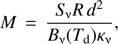 (2)
(2)
where R is the gas-to-dust ratio and d the distance towards the clump.
3. Extinction mapping technique
We employ the technique from Kainulainen & Tan (2013), which is based on combining extinction maps made at two wavelength regimes: in NIR using NICER (Near-Infrared Color Excess Revisited, Lombardi & Alves 2001) and in MIR using the absorption against the Galactic background (e.g., Peretto & Fuller 2009; Butler & Tan 2012). Below, the implementation of the two techniques is explained in detail.
3.1. NICER method
We use the NICER method in conjunction with JHKS photometric data of the VVV survey. The method is based on NIR color measurements of stars shining through the molecular cloud and comparison of those with stars of a reference field that is (optimally) free from extinction. The observed reddening towards the cloud region is used to estimate the extinction by adopting a wavelength dependent reddening law. The extinction values towards each star are then used to derive a spatially smoothed dust extinction map.
This method is straightforward when applied for nearby clouds (d < 500 pc, e.g., Lombardi et al. 2006; Froebrich et al. 2007; Juvela et al. 2008; Goodman et al. 2009; Kainulainen et al. 2009), where the contamination due to stars between the cloud and the observer is small. The extinction towards more distant clouds might be underestimated because of these (mostly unreddened) foreground stars, especially in high-extinction regions where the fraction of foreground sources is high (Lombardi 2005). The foreground stars do not trace the dust reddening caused by the cloud, but only the reddening along the line of sight until the cloud. Therefore, foreground sources should be removed as accurately as possible, which is challenging in practice because of the degeneracy between the intrinsic colors of stars and reddening caused by extinction.
The subtraction of the foreground is also necessary for the reference field (see, Kainulainen et al. 2011). Due to diffuse dust in the Galactic plane, stars in the reference field, located at the same distance as stars behind the cloud, are redder than the ones at closer distance. Therefore, foreground stars shift the mean color of the reference field towards blue, which leads to an overestimation of the extinction. For the implementation of the NICER method we have to find a reliable way to remove the effect of the foreground stars. This is described in the following.
First, we derive a “dirty” extinction map using arbitrary reference colors and use this map to identify low- and high-extinction regions. The low-extinction region (Fig. 2; 338.39° < l < 338.58°; −0.36° < b < −0.21°) is then used as a control field to estimate the reference colors, indicating the average star colors without dust reddening by the cloud. In the regions of high extinction, identifying foreground stars is simple: they appear as a distinct feature in the frequency distribution of individual extinction measurements (cf., Kainulainen et al. 2011). For regions of lower extinction the feature is less distinct, but under the assumption of uniformly distributed foreground stars the position and width of the frequency distribution remains the same; this fact can be used to statistically subtract the contribution of foreground stars to the reference field colors. To do this, we fit a Gaussian function, Gfg, to the peak of the foreground stars in the extinction histogram H(AV) (Fig. 3) and subtract these stars in a statistical sense from the distribution. To achieve this, we add a weighting term ( , see Fig. 3) into the original NICER method. This weighting term suppresses the contribution of stars that might be foreground stars, and it is calculated in the following way
 |
Fig. 2. Extinction maps of Nessie derived using the NIR data of the VVV survey (top), MIR data of the Spitzer Space Telescope (center) and their combination (bottom). The black areas indicate regions of bright MIR emission that hampers extinction mapping. The red rectangle marks the area used for estimating the reference colors for the NICER method. The white circle marks the high-extinction region used to estimate the MIR foreground emission. |
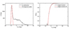 |
Fig. 3. Left: the black line shows a histogram of the calculated extinction from a high-extinction region. The red line marks the Gaussian fitted to the peak of foreground stars. Right: the black line shows the empirical weighting function, which is derived as shown in Eq. (3). The red line shows the fitted function, which is then introduced into the weighting function of the NICER method (Eq. (4)). |
 (3)
(3)
The weighting term is introduced into Eq. (15) of Lombardi & Alves (2001) as shown here: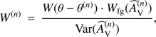 (4)
(4)
where W(n) is the weighting of the nth star, W(θ − θ(n)) is the weight for the distance between the actual location θ and the location of the nth star θ(n),  is the foreground weight based on the estimated extinction of the nth star, and Var(
 ) is variance of the estimated extinction of the nth star.
With this method the contribution of foreground stars was subtracted statistically from the mean color of the reference field to calculate an estimate of the mean color of the stars in the background of the cloud. The statistical subtraction is done in the JHK-color-color space, where the density of foreground stars was subtracted from the density of the reference field stars in each color-color bin. Subsequently, the foreground-corrected number of stars per bin was calculated from the resulting density in the reference field. The foreground-corrected mean color was calculated from this sample of stars, which is also the estimate of the background color. The JHK-color-color histograms of the reference field before and after correction are shown in Appendix C.
With the foreground-corrected reference color and the method for extracting foreground sources, the “true” NIR extinction map was calculated. The spatial resolution of the map is given by the width of the Gaussian smoothing function that is used to smooth the pencil-beam measurements towards the stars onto the map grid. The pixel size is chosen following the surface number density of background sources so that even in high-extinction regions, where the density is lower, each pixel covers at least two stars. For the VVV data we concluded that a pixel size of 24″ is sufficient, which leads to a beam width of 48″.
3.2. Mid-infrared extinction measurement
We use the MIR imaging data from the GLIMPSE survey to estimate extinction through the cloud at 8 μm. Generally, the technique is based on the extinction of the diffuse MIR emission from the Galactic plane by the dust of the cloud (see, e.g., Johnstone et al. 2003; Peretto & Fuller 2009; Butler & Tan 2012). If we consider a simplistic geometry in which the intensity of radiation behind the cloud is I0, the intensity right in front of the cloud is I1 = I0e−τ8, in which τ8 refers to the optical depth at the Spitzer 8 μm band. An observer detects the intensity Iobs,1, which in addition to I1 contains the intensity Ifg that is emitted from between the cloud and the observer, that is, Iobs,1 = I1 + Ifg. A line-of-sight off the cloud does not exhibit extinction and the observed intensity is Iobs,0 = I0 + Ifg. Combining these relations, one can solve the optical depth (5)
(5)
Thus, the optical depth along the line of sight can be estimated through measurements of the off-cloud and foreground intensities.
Various approaches have been used in the past to estimate the off-cloud and foreground intensities (see, e.g., Johnstone et al. 2003; Peretto & Fuller 2009; Ragan et al. 2009; Butler & Tan 2012). We follow an approach similar to Butler & Tan (2012) to which we refer for a thorough description and discussion; we describe here only the implementation of the technique in our case. The off-cloud intensity is estimated using a median-filtered 8 μm map. Prior to the filtering, the most prominent dark features are masked from the map by using a threshold intensity of 46 MJy sr−1. The filter size defines the upper limit of the structures the map is sensitive to. However in our case, we will later combine the MIR-derived map with the NIR-derived map that probes spatial scales larger than 24″. Therefore, the filter function width is not a crucial choice for us, as long as there is some overlap of scales probed by the MIR and NIR maps. Following the discussion in Ragan et al. (2009), we chose the filter width of 3′.
The foreground intensity is estimated with the help of the pixels with lowest intensities (i.e., highest extinctions) in the 8 μm data. If several independent high-extinction regions show similar intensities, one can assume that such locations are opaque and the intensity towards them is a reasonable estimate of the foreground intensity. The smallest intensities detected in the cloud area are Iobs,1 = 24.6 MJy sr−1. There are three independent locations in the cloud where the intensity is within 2σrms of this value (the rms noise, σrms, of the GLIMPSE data is ~0.6 MJy sr−1, Reach et al. 2005). One of them (l, b = 337.895°, −0.563°) is extended, containing tens of pixels, which indicates that the region is indeed saturated. The number of saturated regions is relatively low given the large extent of the cloud on the sky; it would be preferable to have numerous saturated regions along the cloud. Regardless, we adopt the value of 24 MJy sr−1 for the foreground intensity. We note that the resulting fraction of foreground emission, that is, Ifg/Iobs,0 ≈ 45%, well in the range of the foreground intensities typically determined for IRDCs (e.g., Butler & Tan 2012).
Following the estimation of the off-cloud and foreground intensities, Eq. (5) is used to compute an optical depth map for Nessie. Finally, the map is converted into units of visual extinction by adopting the ratio between 8 μm and V band optical depths (based on Cardelli et al. 1989; Ossenkopf & Henning 1994, see Kainulainen & Tan 2013)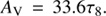 (6)
(6)
The resulting extinction map is shown in Fig. 2.
3.3. Combined near- and mid-infrared extinction measurement
We have now derived the NIR and MIR extinction maps; both show some advantages and disadvantages. The NIR data are sensitive to low column densities, but are at low resolution. The MIR data are at good resolution, but are much less sensitive. Therefore, we now want to combine them and use the NIR data to recalibrate the MIR data, thus gaining high spatial resolution of the MIR data while imposing the good calibration of the NIR data on them. The combination of NIR and MIR extinction maps follows the scheme described in Kainulainen & Tan (2013). The combined maps deliver a higher dynamic range of extinction compared to maps computed from NIR or MIR data alone (Fig. 2). The correlation between the two maps is shown in Appendix D.
The combined map is then converted to molecular hydrogen column density by applying the conversion of Savage et al. (1977), Bohlin et al. (1978), Rachford et al. (2002): (7)
(7)
using a typical reddening constant of RV = 3.1 (Schultz & Wiemer 1975) and assuming all hydrogen atoms are in molecular form.
4. Results
4.1 Distance determination
The foreground star density measurements (see Sect. 3.1) allow us to estimate the distance of Nessie independently of previous, kinematic distance estimates. We can compare the measured surface density of foreground stars with a distance-dependent stellar surface density model of the Galaxy. We used the Besançon Galactic stellar distribution model (Robin et al. 2003) to estimate the distance; see Fig. 4. For a more detailed description of the method see Kainulainen et al. (2011) and Ioannidis & Froebrich (2012). The most important input parameter of the stellar distribution model is the extinction caused by diffuse interstellar dust. We used the measurements by Marshall et al. (2006) to estimate the mean extinction along the line of sight towards Nessie. For an estimate of the uncertainty we also estimated the minimum and maximum extinction, which indicate the upper and lower limits of the surface density (Fig. 4). We neglected other, potentially significant uncertainties in our distance calculations such as the uncertainty of the measured number surface density of the foreground stars or of the stellar distribution model. Therefore, the uncertainty of the distance is underestimated and it is more likely to be on the order of 15 % corresponding to Δd ≈ 0.5 kpc (Kainulainen et al. 2011).
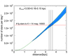 |
Fig. 4. Predicted stellar surface density based on the Besançon stellar distribution model (Robin et al. 2003). The blue area indicates the uncertainty arising from the scatter in the diffuse extinction measurements. The horizontal line represents the measured foreground star surface density and the vertical lines the resulting estimates of the distance and its uncertainty. |
The result of our distance estimate is dextinction = 3.5 ± 0.5 kpc, which is in agreement with the kinematic distance estimations of Jackson et al. (2010), dHCN = 3.1 kpc. We find also dynamical distance measurements from Wienen et al. (2015) for 14 ATLASGAL sources likely embedded in the Nessie cloud. Their distances range between 3.0 kpc and 3.5 kpc, which is also in agreement with our estimate. The distance of ~3.5 kpc suggests that Nessie is associated with the Scutum-Centaurus spiral-arm of the Milky Way as suggested by Goodman et al. (2014) and Ragan et al. (2014).
4.2. The large-scale structure
The combined NIR and MIR extinction map of the Nessie cloud is shown in Fig. 5 and zoom-ins in Figs. 6–8. For comparison, Fig. 2 shows the NIR-based map, MIR-based map, and their combination.
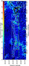 |
Fig. 5. Column density map of the Nessie filament. The white polygon marks the area chosen for the mass estimate of the cloud. The green rectangles show the positions of the zoom-ins shown in Figs. 6–8. |
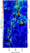 |
Fig. 6. Zoom-in number one of the column density map (Fig. 5). The black contours indicate the levels of 5, 10, 20, 30, 40, 50, 60 × 1021 cm−2. The white contour indicates the smoothed AV = 3 mag level. Additionally, the Class1 (“×”) and Class2 (“+”) YSOs are marked in white. |
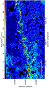 |
Fig. 7. Zoom-in number two of the column density map (Fig. 5). The black contours indicate the levels of 5, 10, 20, 30, 40, 50, 60 × 1021 cm−2. The white contour indicates the smoothed AV = 3 mag level. Additionally, the Class1 (“×”) and Class2 (“+”) YSOs are marked in white. |
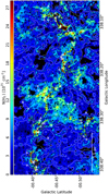 |
Fig. 8. Zoom-in number three of the column density map (Fig. 5). The black contours indicate the levels of 5, 10, 20, 30, 40, 50, 60 × 1021 cm−2. The white contour indicates the smoothed AV = 3 mag level. Additionally, the Class1 (“×”) and Class2 (“+”) YSOs are marked in white. |
The filament has a length of ~1.1° following the central, dense main axis (neglecting inclination) and a perpendicular width of ~0.05°. This corresponds to a physical size of 67 pc × 3 pc at a distance of d = 3.5 kpc. The width of the extinction structures, defined at the column density contours of about AV = 3 mag, varies along the filament. This can be seen in the zoomed-in map of Nessie (Fig. 6). In the region in the range 338.57° < l < 338.95° the low-column-density material is located only towards the south of the dense main axis, in the range 338.23° < l < 338.30° towards north and south, and the rest of the filament shows almost no surrounding low column density material. These two low-column-density regions also show some less dense structures, which are mainly orientated almost perpendicular to the main filament.
We need to identify which structures that we see in the map are actually part of Nessie. This is difficult because we miss information about the line-of-sight velocities of the structures. However, the Nessie filament was confirmed as a velocity coherent structure by Jackson et al. (2010). Additionally, some areas lack the MIR extinction data and cannot be used in the further analysis, such as the HII-bulb at (l; b) = (337.95°; −0.46°) (Fig. 5), which is part of Nessie in Jackson et al. (2010). Therefore, the map needs to be cropped to the Nessie filament. To do this, we introduce a polygon around the cloud (see Fig. 5). The area selection is mainly based on physical inspection of the derived column density map with orientation on the AV = 3 mag contour and the observations published by Jackson et al. (2010).
We derive an estimate of the total cloud mass from the column density map, given by: (8)
(8)
where N(H2)i,j is the column density of the (i, j) pixel of the map, p = tan (1.2″) × dNessie is the physical size of a pixel, mH is the mass of the hydrogen atom, and μH2 = 2.8 the mean molecular weight of the interstellar medium (Kauffmann et al. 2008). The total mass of the Nessie cloud within the polygon (Fig. 5) is MNessie = 4.2 × 10⁴M⊙.
From the length and mass, we calculate the mean linemass of the filament (mass per unit length along the main axis of the filament). The mean line-mass of Nessie is (M/l) = 627 M⊙ pc−1. As we neglected an inclination of the filament, which would increase its length, the derived line-mass is an upper limit. We note that there are variations in the line mass along the filament, both at large scales due to the varying amount of diffuse extinction and at small scales due to the substructure of the cloud.
4.3. Fragmentation analysis
We analyzed fragmentation of Nessie simultaneously over a wide range of spatial scales using an algorithm explained in Kainulainen et al. (2014), which employs wavelet filtering to identify structures at various spatial scales. In short, the algorithm uses a spatial filtering algorithm based on the ã Trous wavelet transform (Starck & Murtagh 2002) to decompose the column density map into scale-maps that describe structure at different scales. The different scales are defined as 2i pixels, with 2 ≤ i ≤ 8, where the limits are given by the pixel size for small scales and the cloud size for large scales. Individual structures are then identified from each scale map using the clumpfind-2D algorithm (Williams et al. 1994). This provides the position, the size in x and y direction, and the total amount of column density of the structures N(H)tot.
For reliable detection of structures, it is necessary to estimate the noise level of each scale map. The noise level is estimated as the standard deviation σ of an (almost) extinction-free area. The size of the area corresponds to the size-scale of the largest scale map. To test the robustness of the structure identification, we tested the clumpfind-2D algorithm for contour level separations of 1.5σ, 3σ, 4σ and 5σ with the lowest level at 3σ. The results do not show a significant difference and we chose the level separation of 3σ.
The numbers of structures identified at each scale using the chosen technique are listed in Table 1. The number of structures increases towards smaller scales, but drops significantly for the smallest scales (i = 2, see Table 1). This behavior was seen for all tested algorithm parameters and therefore is not likely to be an artifact. In the data these smallest structures trace only the densest clumps, which are predominantly located along the dense spine of the filament, but not in the surrounding low-column-density gas. This suggests that only in the densest parts is the filament able to fragment into the smallest scales.
Table 1 shows the properties of structures at each scale i: the total number of identified structures Nstrc, the total mass of these structures Σ (Mstrc), the median hydrogen number density ñ(H), and the median separation s̃. The sum of the masses over all scales, including scale i > 8, results in a total cloud mass of about 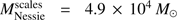 . This is slightly higher than the mass derived from the combined column density map (see Sect. 4.2). The difference is a consequence of the spatial filtering algorithm used, which may not accurately reproduce the true shapes of the structures.
We include in the fragmentation analysis all structures identified at scales i = 2–8 and only include structures within the Nessie filament area (see the polygon in Fig. 5). We computed the projected nearest neighbor distances of the structures. The separation distributions of the scales i = 2, 3 are shown in Fig. 9. They are non-Gaussian in shape and we adopt the median separation as a diagnostic of the separations (given in Table 1).
 |
Fig. 9. Distributions of the separations (left) and densities (right) of the structures identified from the scale maps i = 2 (top) and i = 3 (bottom). The dashed line indicates the median and the dotted lines the 95% quantiles of each distribution. |
For the fragmentation analysis an estimate of the structure density is interesting; we estimate this from the outputs of the clumpfind-2D algorithm. The size of a structure was given by clumpfind-2D as the number of pixels, Npix, in the FWHM area. For the calculation of the structure volume we assume the shape of a prolate spheroid, that has been found to be among the shapes that best quantify the structures at the scales we are looking at (e.g., Kainulainen et al. 2014). The depth of the prolate spheroids is estimated as the shorter of the projected x and y dimensions. Therefore, the volume of a fragment is (9)
(9)
The average column density, N̄(H), is given by: N̄(H) = N(H)tot/Npix, and therefore, the hydrogen number density of one structure is: n(H) = N̅(H) × π × x × y/V. The median number density and the 95% interval for structures at each scale are shown as a function of their median separation in Fig. 10.
 |
Fig. 10. Median number density of structures at different spatial scales as a function of their median separation. Measurements of this study are marked with crosses. The square marks the data point derived from HNC observations of Jackson et al. (2010). The error bars show the 95% quantiles of both measurements. The blue lines indicate the scale dependency of an infinitely long cylinder in the non-turbulent case (solid), and non-thermal case (dash-dotted), and the dashed red line indicates the scale dependency of Jeans’ fragmentation. The black line shows a power-law fit to the data. |
Additionally, we estimated the median separation and density from the HNC molecular line observations of Jackson et al. (2010). We used the shown positions to estimate their separation at the distance of d = 3.5 kpc. The density was calculated assuming a spherical geometry with a radius of  , using the angular size Ω of the identified clumps, and their mass M. The hydrogen number density is given by:
 (10)
(10)
where μH = 1.4 is the mean molecular weight of the interstellar medium with respect to atomic hydrogen and mH is the mass of a hydrogen atom.
We estimated the uncertainty of the median separations and median mean densities using bootstrapping, because their probability distributions are not Gaussian (see Fig. 9). For the separation and mean density on every scale, we drew a new sample of values from among the observed values of separations and mean densities. This new sample had the same amount of data points as originally detected at that scale. We then calculated the median of these new simulated samples. The resulting distribution of the median values then estimates the sampling function of the observed median and was used to estimate the uncertainty using the standard deviation. The uncertainties vary between 1 and 14% for the separation and between 1 and 25% for the density on scales of i = 3 and i = 8. The uncertainty values of all scales are given in Table 1.
The scatter shown in the separation density plot represents the 95% quantiles of the measured parameters. Large uncertainties, which are neglected here, are the opacity at different wavelengths (J, H, K, 8 μm) and their ratios contributing in the extinction measurement and the conversion factor from extinction to column density. For measuring masses, the uncertainty of the distance, as discussed before, also introduces a significant contribution. For more detail, see Kainulainen et al. (2011), Kainulainen & Tan (2013).
The density-separation relation (Fig. 10) shows a clear decrease of the mean densities for larger separations. We perform a linear least-square-fit in the log-log space to the data, which represents a power law of the form ñ(H) = A × s̃p as log(ñ(H)) = p × log(s̃) + log(A).
The resulting parameters are p = −0.96 ± 0.05 and log(A) = 3.22 ± 0.02, which is  . The fitted model is shown as a black line in Fig. 10.
A commonly used fragmentation model is the spherical Jeans’ instability model (Jeans 1902), where the separation is linked to the mean density ρ̃ via the Jeans’ length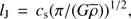 (11)
(11)
where cs is the sound speed within the medium, and G the gravitational constant. We compute the prediction from this assuming a gas temperature of T = 15 K. At all scales, the observed mean separations are in agreement with the Jeans’ scale within a factor of approximately three. However, for the smallest scales, i = 2–4, the measurements are systematically below the predicted relationship and for the largest scales, the measurements are systematically above (see the discussion about the slope of the relationship later in this section).
A shallower slope of the Jeans’ fragmentation can be achieved by assuming a non-isothermal medium (e.g., Takahashi et al. 2013). The innermost dense (~104 cm−3) regions of the cloud are shielded from the interstellar radiation field and therefore, can reach temperatures down to 10 K. As the surrounding low-density gas (~102 cm−3) is exposed to the radiation, we assume a higher temperature of 20 K. This leads to a slope of about −1.7, which still does not solve the systematic deviations from the observation.
Another commonly used model describes the fragmentation of an infinitely long, self-gravitating cylinder (Chandrasekhar & Fermi 1953; Inutsuka & Miyama 1992). This model predicts the separation, λ, depending on the scale-height H = σv(4πGρc)−1/2, where ρc is the central density of a filament in virial equilibrium, σv the velocity dispersion of the medium, and G the gravitational constant. In the case of a non-turbulent medium, the velocity dispersion σv is given by the sound speed cs within the medium (we assume T = 15 K to calculate the sound speed). In the regime of the filament radius, R ≫ H, the separation is given by λ = 22 H. If we assume a central density at the largest scale of nc(H) ≈ 103 cm−3, then we derive a scalehight of H ≈ 0.15 pc. This is smaller than the typical radius of Nessie, R ≈ 1.5 pc (see Sect. 4.2). Therefore, the separation is predicted to be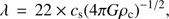 (12)
(12)
which is shown in Fig. 10 and is in agreement with the measurements within a factor of approximately three for scales larger than i = 5, but systematically above the measured densities. However, the model predicts central densities while we derived mean densities, and therefore, the model predicts an upper limit of the mean densities.
The above models describe fragmentation in non-turbulent medium. However, observations show that high-line-mass filaments have a non-thermal line width (Jackson et al. 2010; Kainulainen et al. 2013), which is higher than the sound speed cs in the non-turbulent case. Larson (1981) found a relation between the size of a molecular cloud and its observed line width. Such a line width-size relation might also apply to the structures observed here, and therefore we adopted a typical relation of σv = 0.72 km s−1 × (λ/1 pc)0.5 (Solomon et al. 1987; Heyer & Brunt 2004; Pillai et al. 2006; Shetty et al. 2012; Colombo et al. 2015), where the line width σv depends on the observed size scale λ. The non-thermal line width exceeds non-turbulent motion, given by the sound speed cs, at large scales. But the line-width-size relation can also be partially explained by the non-isothermal behavior of the gas.

where ρc is the central density of a filament in virial equilibrium, and G the gravitational constant (Fig. 10).
Therefore, the relation between the central density and the separation is ρc∝ λ−1, which is in agreement with the observed slope of p = −0.96 ± 0.05. However, again we have to mention that the model predicts central densities while we derived mean densities. Additionally, without information about the kinematics of the cloud, we cannot constrain the scaling velocity of the line-width-size relation.
Results of the fragmentation analysis.
4.4. Comparison with ATLASGAL
We briefly describe how the parsec-scale structures identified in Nessie from ATLASGAL data (resolution of 18″, Schuller et al. 2009) break down into substructures when extinction data offer about ten times higher resolution. For this, we considered the 16 sources from the ATLASGAL GCSC catalog (Csengeri et al. 2014) that are likely embedded in the cloud. We calculated the number of structures within the FWHM ellipse of the ATLASGAL sources at the two smallest scales (i = 2, 3) of the extinction map (see Fig. 11). We also estimated the mass of the ATLASGAL clumps by adopting Eq. (2) and assuming a dust temperature of Td ≈ 15 K. These masses are then compared to the total mass of the small-scale structures. The resulting ratios are shown in Table 2.
 |
Fig. 11. Combined NIR and MIR extinction map (l = 338 × 10°, b = −0.45°) overlaid with the half power contour of two ATLASGAL GCSC sources (black ellipses) and their covered sources identified with clumpfind-2D from the scale 2 map. The white lines show the contours of the ATLASGAL emission. |
In particular, we found that, on average, the number of small-scale structures within the half power ellipse of the clump is N̅strc,2 = 2.9 and N̅strc,3 = 2.8. These contain 2% and 6% of the mass of the ATLASGAL clump. The half power ellipses of the clumps and the i = 2 structures identified within the clumps are shown in Fig. E.1 overlaid on the extinction map. While half of the ATLASGAL clumps are clearly associated with high-extinction peaks, the four most massive ones (>500 M⊙) in particular contain no or only low-extinction peaks. This is dominantly because of the caveats of the extinction mapping technique. The massive clumps commonly exhibit MIR emission of polycyclic aromatic hydrocarbons (PAHs) in the 8 μm band (Benjamin et al. 2003); this interferes with the extinction mapping procedure. Also bright foreground stars cause a lack of MIR extinction and influence our results. In total, this likely leads to an underestimated number of substructures per clump and to underestimation of some of their masses. This also shows that our method is excellent for identifying the youngest and densest regions, but it starts to fail as soon as star formation progresses and the regions show strong MIR emission.
ATLASGAL GCSC clumps (Csengeri et al. 2014) likely embedded in the Nessie cloud.
5. Discussion
5.1. Scale-dependent fragmentation of Nessie
In the following, we discuss the scale-dependent fragmentation of Nessie (Fig. 10) in the context of the analytic gravitational fragmentation models. We showed that the upper limit of the average line-mass of Nessie is (M/l) = 627 M⊙ pc−1. For a thermally supported filament at a temperature of T = 15 K, the critical line-mass is (M/l)crit = 20 M⊙ pc−1. Thus, the filament is clearly thermally supercritical. There are no analytic theories that would self-consistently explore the evolution of such highly thermally super-critical filaments.
In the absence of directly applicable models, a common approach in the recent literature is to assume that the non-thermal motions provide a straightforward, idealized supporting force for the filament, increasing its critical line-mass (e.g., Jackson et al. 2010; Hernandez et al. 2012; Busquet et al. 2013; Beuther et al. 2015). This commonly leads to a conclusion that the line-masses of high-line-mass filaments are close to their critical line-masses. This is also true for Nessie. Jackson et al. (2010) showed that the non-thermal motions in Nessie increase the critical line mass to (M/l)vir = 525 M⊙ pc−1, which is similar to our observed value.
Building on the above agreement, observations are commonly compared to the predictions of gravitational fragmentation models developed for near-equilibrium cylinders. These models typically proceed from a static initial configuration with a linear perturbation analysis. In short, such models predict a periodic fragmentation pattern with a specific wavelength, that is, the fragmentation pattern predicted by the models is not scale-dependent. However, the fragmentation wavelength depends on the density of the filaments as described by Eqs. (13), (12), and (11); filaments with different densities have different fragmentation wavelengths. This should be kept in mind when interpreting the relationship between the data and models presented in Fig. 10.
In this context, the observed slope of the mean density-separation relationship in Nessie is in agreement with that of a non-thermal, self-gravitating cylinder that has a Larson-like line-width-size relation (σv∝ λ0.5, Larson 1981; Solomon et al. 1987; Heyer & Brunt 2004; Shetty et al. 2012; Colombo et al. 2015). As the cloud shows non-thermal velocity dispersions (Jackson et al. 2010), this relation could be a result of turbulent motions within the cloud, but also systematic motions, such as collapse, could affect the line width. The observed median nearest-neighbor separations of the fragments are within a factor of two of the predictions of the isothermal and non-isothermal Jeans’ fragmentation (Jeans 1902). However, the slope is significantly steeper than the observed one. Additionally, on the large scales, the separations are also in agreement with the fragmentation model of a non-turbulent, self gravitating, infinitely long cylinder (Chandrasekhar & Fermi 1953; Inutsuka & Miyama 1992), but again the slope of the model is significantly steeper than observed. We note that the cylindrical models predict central densities, which can only be seen as upper limits for the derived mean densities.
Previously, a change of fragmentation mode between large and small scales has been seen at the size-scale of ~0.5 pc, for example, in the studies of the young high-mass cloud G11.11-0.12 (Kainulainen et al. 2013), the Taurus cloud (Hacar et al. 2013), and the integral-shaped filament in Orion (Teixeira et al. 2016; Kainulainen et al. 2017). While we do not detect one in Nessie, the data are in agreement with the presence of such a feature, that is, we cannot rule it out (c.f., Fig. 10). One possible explanation for the change of fragmentation modes could be changing influence of the environment (Pon et al. 2011). While on large scales, fragmentation is driven by the characteristics of the cylindrical, filamentary structure, the smaller scales approach a more spherical shape, which is independent of larger scales. Also, recent numerical simulations have explored possibilities to explain scale-dependent fragmentation through dynamical processes (e.g., Clarke et al. 2017; Gritschneder et al. 2017).
5.2. Star formation potential
Ultimately, one would like to link the fragmentation in Nessie to star formation. To take the first step towards this, we estimated the young stellar object (YSO) content of Nessie using publicly available multi-band photometric catalogs. The detailed methods used to identify the YSOs and estimate the SFR are explained in Zhang et al. (2018). Here we give a short description of the method.
For the YSO selection, we used NIR data (we did the PSF photometry on VVV images, VISTA Variables in the Via Lactea, Saito et al. 2012), Spitzer GLIMPSE (Galactic Legacy Mid-Plane Survey Extraordinaire, Benjamin et al. 2003; Churchwell et al. 2009) and MIPSGAL (Multiband Imaging Photometer Galactic Plane Survey, Carey et al. 2009; Gutermuth & Heyer 2015) archival catalogs, the AllWISE catalog (Wide-field Infrared Survey Explorer, Wright et al. 2010), the Herschel Hi-GAL catalog (Herschel infrared Galactic Plane Survey, Molinari et al. 2010, 2016), the Red MSX source catalog (Midcourse Space Experiment, Lumsden et al. 2013, used to include massive protostars), and the methods from Gutermuth et al. (2009), Koenig & Leisawitz (2014), Saral et al. (2015), Robitaille et al. (2008) and Veneziani et al. (2013). Our YSO selection scheme uses the SEDs of sources from 1 to 500 μm and can efficiently mitigate the effects of contamination. In Nessie, we finally obtain 298 sources with the excessive IR emission, of which 35 are classified as AGB candidates using the multi-color criteria.
Considering the distance of Nessie, it is necessary to correct the flux densities of the YSO candidates for extinction. We use the method suggested by Fang et al. (2013) and Zhang et al. (2015) to estimate the foreground extinction towards each YSO candidate and de-redden their photometry. Here we also give a short description of this method.
-
For the sources with J, H, KS detections, the extinction is obtained by employing the JHKS color–color diagram. Figure 12 shows the J–H versus H–KS color–color diagram of the YSO candidates in Nessie. Given the different origins of intrinsic colors of YSO candidates, the color-color diagram is divided into three subregions. In region 1, the intrinsic color of [J–H]0 is simply assumed to be 0.6; in region 2, the intrinsic color of a YSO is obtained from the intersection between the reddening vector and the locus of main sequence stars (Bessell & Brett 1998); and in region 3, the intrinsic color is derived from where the reddening vector and the classical T Tauri star (CTTS) locus (Meyer et al. 1997) intersect. The extinction values of YSO candidates are then estimated from observed and intrinsic colors with the extinction law of Xue et al. (2016).
-
For other sources (outside these three regions or without detections in JHKS bands), their extinction is estimated with the median extinction values of surrounding Class II sources that have extinction measurements in step 1.
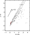 |
Fig. 12. The H–KS vs. J–H color–color diagram for the YSO candidates in Nessie. The solid curves show the intrinsic colors for the main sequence stars (black) and giants (red; Bessell & Brett 1998), and the dash–dotted line is the locus of T Tauri stars from Meyer et al. (1997). The dashed lines show the reddening direction, and the arrow shows the reddening vector. The extinction law we adopted is from Xue et al. (2016). We note that the dashed lines separate the diagram into three regions marked with numbers 1, 2, and 3 in the figure. We use different methods to estimate the extinction of YSO candidates in different regions (see the text for details). |
Using the de-reddened SEDs, we re-classify the YSO candidates into Class I, Flat, and Class II sources based on their spectral indices and bolometric temperatures (Greene et al. 1994; Chen et al. 1995). Figure 13 shows the KS − [8.0] versus J–H color–color diagrams before and after de-reddening for Class I+Flat and Class II sources in Nessie.
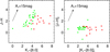 |
Fig. 13. The observed (left panel) and de-reddened (right panel) KS −[8.0] vs. J–H color-color diagrams for Class I+Flat (red) and Class II (green) sources in Nessie. The black arrows show the extinction vectors. |
Although we have removed some contamination during the YSO selection process, our YSO candidates in Nessie are still contaminated by the foreground and background sources.
The foreground contamination mainly includes the foreground AGBs and the foreground YSOs which are associated with the molecular clouds that are located between us and Nessie. We use the AV values of YSOs obtained previously and the 3D extinction map (Marshall et al. 2006) to isolate the foreground contamination. Based on the distance of Nessie, we can estimate the foreground extinction in different lines of sight towards Nessie with the 3D extinction map. If the extinction value of a YSO is lower than the corresponding foreground extinction of Nessie, this YSO would have a high probability of being a foreground contamination. We checked the YSOs in Nessie and marked the possible foreground contamination using this method. The fraction of foreground contamination in Nessie is 10% in Class I+Flat sources and 9% in Class II sources.
Our YSOs are also contaminated by background sources, including extragalactic objects, background AGBs, and background YSOs which are associated with the molecular clouds that are located behind Nessie. We think that the extragalactic contamination is not important in our YSOs because we are observing through the Galactic plane. Many background AGBs have been removed using the multi-color criteria during the YSO identification process. The residual contamination of background AGBs is estimated with the control fields. We select five nearby fields with weak CO emission as the control fields and apply the YSO selection scheme to all the control fields to select YSOs. Assuming that there is no YSOs in each control field, all selected “YSOs” in the control fields are actually contamination by AGBs (if neglecting the extragalactic contamination). With an assumption of a uniform distribution for AGB stars, we can estimate the number of residual background AGBs in the Nessie using the mean value of the surface density of background AGBs in five control fields. Combining the numbers of background AGBs identified by color criteria and estimated using control fields, we found that the fraction of background contamination is 22% in Class I+Flat sources and 11% in Class II sources. We note that we did not try to eliminate the contamination from background YSOs because they are difficult to remove without the information of radial velocities of YSOs.
After removing the contamination, we obtain 51 Class I and flat spectrum objects and 137 Class II sources in Nessie. In order to calculate the SFR, we must estimate the total mass of YSOs in Nessie. In this work, we use different methods to estimate the total mass of Class I+Flat and Class II populations:
-
We use the de-reddened photometry of Class II sources in Nessie to estimate the flux completeness. Figure 14 shows the KS absolute magnitude histogram of Class II sources in Nessie. We simply adopt the peak position of histogram as the completeness of KS band (~1 mag). Figure 15 shows the MKS − M* relation for Class II sources constructed from YSO models presented by Robitaille et al. (2006). Using this relation, we transfer the KS band completeness to the mass completeness of 1.48 ± 0.65 M⊙. Assuming a universal IMF (Kroupa 2001), we estimated the number of Class II sources to be
 and the total mass of Class II sources to be
  .
. -
For Class I+Flat sources, we used the observed luminosity functions constructed by Kryukova et al. (2012) as the template to estimate the total number of Class I+Flat sources. We calculate the bolometric luminosities of Class I+Flat sources using the trapezoid rule to integrate over the finitely sampled de-reddened SEDs (Dunham et al. 2008, 2015). Figure 16 shows the the de-reddened luminosity function of Class I+Flat sources in Nessie and the corresponding luminosity completeness, which is calculated with the method suggested by Kryukova et al. (2012), is also marked with the red line. As a comparison, we also plot the luminosity function of Class II sources in Nessie. Assuming a universal luminosity function, we estimate the total number of Class I+Flat sources in Nessie to be
 . Assuming the average mass of 0.5 solar mass for each Class I/Flat source, we estimated the total mass of Class I+Flat sources to be
  .
.
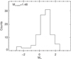 |
Fig. 14. KS absolute magnitude (MKS) histogram of Class II sources in Nessie. |
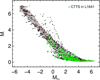 |
Fig. 15. The relation between stellar mass and KS absolute magnitude of Class II sources. The black dots represent the Robitaille et al. (2006) Stage 2 models with 0.001 < Mdisk/M* < 0.01, 0.08 < M* < 7 M⊙, and 30° < inclination angle < 60°. The red curve shows the robust polynomial fitting while the gray region shows the 1σ uncertainty of the fitting. The CTTS in L1641 from Fang et al. (2013) are marked with green filled circles. Most of CTTS are located in the gray region, which confirms that this MKS − M* relation for Class II sources is consistent with the observational results. |
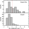 |
Fig. 16. De-reddened luminosity functions of Class I+Flat (top panel) and Class II (bottom panel) sources in Nessie. The red vertical line shows the de-reddened luminosity completeness. |
Adopting the lifetime of Class II sources, 2 Myr (Evans II et al. 2009), as the star formation time-scale, we obtain 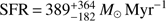 for Nessie. The SFE within the star-forming time-scale is estimated by the total mass of YSOs, MYSOs, and the gas mass of Nessie,
  . The uncertainty is mainly from the uncertainty of transferring Ks magnitudes to stellar masses and the small number of observed Class I and Class II sources. To place these values in context, the SFR of Nessie is comparable to those of the most active nearby star forming regions like Perseus (150 M⊙ Myr−1), Orion A (715 M⊙ Myr−1) and Orion B (159 M⊙ Myr−1; all values from Lada et al. 2010).
It is immediately interesting to compare this direct SFR estimate to other measures commonly linked with the star formation potential of molecular clouds. One such measure is the mass of dense gas in the cloud (e.g., Kainulainen et al. 2009; Lada et al. 2010). Specifically, Lada et al. (2010) found that in the Solar Neighborhood clouds (distance ≲ 500 pc), SFRs correlate best with the mass above a column density threshold of AV ≈ 7.3 mag. Adopting this threshold results in the dense gas mass of Mdg = 8.7 × 10³M⊙ in Nessie. Following the prescription of Lada et al. (2010) for the Solar Neighborhood clouds, the SFR of 4.6 × 10⁻⁸ yr−1 × Mdg = 400 M⊙ Myr−1 follows. This is in agreement with the SFR derived from the YSOs; in Nessie the mass of dense gas above AV ≈ 7.3 mag is a reasonable predictor of the SFR.
Yet another measure commonly connected with SFR is the dense core population of the molecular clouds (e.g., Motte et al. 1998; Alves et al. 2007; Marsh et al. 2016). To analyze this population in Nessie, we can take advantage of the high spatial resolution of our column density map: we can directly count the cores that might form stars or multiple stellar systems and estimate their mass. The mass enclosed in the dense structures smaller than ~0.1 pc is likely to take part in star formation processes. Therefore, the number of structures at the smallest scale of the wavelet-filtered map (i = 2, ~0.08 pc) provides a first-order estimate for the number of stars forming in the cloud in the near future. To account for possible accretion processes during the collapse of a core, we assume that the gas at the scales i = 2 and i = 3 (size < 0.16 pc) can participate in the collapse. This will then give an upper limit for the mass available for star formation. The mass of stars formed by these cores is then estimated by assuming an SFE of 30% (e.g., Alves et al. 2007; Rathborne et al. 2009; André et al. 2010). This results in the stellar mass of Mi = 2,3 = 409 M⊙. Adopting again the star formation time of tSF ≈ 2 Myr leads to a SFR of M*/tSF = 205 M⊙ Myr−1 for the Nessie cloud. This estimate is within a factor of two of the values derived previously. We can also simply use the number of detected cores to gain a crude estimate of the star formation potential. If we assume that each structure at scale i = 2 will form at least one star, Nessie will form 523 stars. This is within a factor of two of the actual number of (completeness corrected) Class I and II sources. If we further divide the total mass in the cores in Nessie by 523, the predicted average mass of a star of 0.78 M⊙ follows; this is relatively close to the mean stellar mass of 0.5 M⊙ of the initial mass function (e.g., Kroupa 2002). Altogether, the above considerations suggest that the dense core population identified from Nessie using the approach of this paper is a reasonable proxy of Nessie’s star formation potential.
5. Conclusions
We analyzed the column density structure of the (projected) 67 pc long filamentary Nessie cloud using a combined NIR and MIR extinction-mapping method on data of the VVV survey and 8 μm Spitzer/GLIMPSE images. Our results are as follows:
-
We derived a high-resolution (~0.03 pc), high dynamic range (N(H2) = 3–100×1021 cm−2) column density map for Nessie and estimated the distance towards it to be d = 3.5 kpc based on NIR source-counts. The mass of Nessie is 4.2 × 10⁴M⊙, considering regions above N(H2) ≳ 3 × 1021 cm−2. This leads to a mean line-mass of about 627 M⊙ pc−1.
-
We analyzed the fragmentation of the cloud across a wide range of scales in the range 0.1–10 pc and detected fragmentation at all scales. We characterize the fragments and find that their masses decrease and densities increase as a function of size-scale. At the smallest scale, the typical masses of the fragments are 0.4 M⊙ and mean densities are ~104. The mean densities of the fragments decrease with their nearest-neighbor separations, following approximately a power-law with an exponent of −0.96±0.05. The previous determination of the 4 pc fragmentation length by Jackson et al. (2010) is in agreement with this relationship, however, our data show that determining the fragmentation length at any one particular scale does not capture the full, scale-dependent picture of fragmentation in Nessie.
-
In the context of analytic gravitational fragmentation models, the observed nearest-neighbor separations are within a factor of two of the Jeans’ length at all size-scales. However, the slope of the observed mean density – separation relationship is significantly shallower than the scale-dependency of the Jeans’ length. The observed relationship is in agreement with a gravitationally fragmenting near-equilibrium cylinder that is supported by non-thermal motions that exhibits a Larson-like velocity-size scaling, that is, a power-law with an exponent of 0.5. This scaling could result, for example, from turbulent motions in the cloud, because the cloud shows clearly non-thermal velocity dispersions (Jackson et al. 2010).
-
We estimated the SFR of Nessie to be 389 M⊙ Myr−1 based on the number of identified YSOs in the cloud. An estimate based on the number of ~0.1 pc-scale column density “cores” yields 205 M⊙ Myr−1. We also estimate the SFR based on the total amount of dense gas (AV > 7.3 mag; Lada et al. 2012) in the cloud, resulting in 400 M⊙ Myr−1. These results suggest that both the number of dense cores and the amount of dense gas above AV > 7.3 mag are relatively good proxies of the star-forming content of Nessie. We further derive the SFE of 0.018 for Nessie. These numbers indicate that the star-forming content of Nessie is similar to the Solar neighborhood giant molecular clouds like Orion A.
-
The ATLASGAL clumps identified in Nessie typically harbor two to three small-scale structures (<0.16 pc). These structures contain about 7% of the mass of the parental clump. However, this is a lower limit as the extinction mapping is susceptible for incompleteness arising from MIR bright objects, such as foreground stars, and warm/hot gas.
We showed that the filamentary Nessie cloud has scale-dependent fragmentation characteristics. These characteristics are in agreement with some of the predictions of gravitational fragmentation models. However, self-consistent scale-dependent fragmentation models are needed to gain understanding of the structure and evolution of filamentary clouds.
Acknowledgments
We thank the referee for constructive comments. M. M. is supported for this research through a stipend from the International Max Planck Research School (IMPRS) for Astronomy and Astrophysics at the Universities of Bonn and Cologne. The work of J. K. was supported by the Deutsche Forschungsgemeinschaft priority program 1573 (“Physics of the Interstellar Medium”). This project has received funding from the European Union’s Horizon 2020 research and innovation program under grant agreement No 639459 (PROMISE). H. B. acknowledges support from the European Research Council under the Horizon 2020 Framework Program via the ERC Consolidator Grant CSF-648505. M. Z. acknowledges support from the National Natural Science Foundation of China (grants no. 11503086). This research has made use of the NASA/IPAC Infrared Science Archive, which is operated by the Jet Propulsion Laboratory, California Institute of Technology, under contract with the National Aeronautics and Space Administration. This work is based on observations made with ESO Telescopes at the La Silla Paranal Observatory under programme ID 179.B-2002. The ATLASGAL project is a collaboration between the Max-Planck-Gesellschaft, the European Southern Observatory (ESO) and the Universidad de Chile. It includes projects E-181.C-0885, E-078.F-9040(A), M-079.C-9501(A), M-081.C-9501(A) plus Chilean data.
References
- Abreu-Vicente, J., Ragan, S., Kainulainen, J., et al. 2016, A&A, 590, A131 [NASA ADS] [CrossRef] [EDP Sciences] [Google Scholar]
- Alves, J., Lombardi, M., & Lada, C. J. 2007, A&A, 462, L17 [NASA ADS] [CrossRef] [EDP Sciences] [Google Scholar]
- André, P., Men’shchikov, A., Bontemps, S., et al. 2010, A&A, 518, L102 [NASA ADS] [CrossRef] [EDP Sciences] [Google Scholar]
- André, P., Di Francesco, J., Ward-Thompson, D., et al. 2014, Protostars and Planets VI: From Filamentary Networks to Dense Cores in Molecular Clouds (Tucson: Univ. of Arizona Press) [Google Scholar]
- Arzoumanian, D., André, P., Didelon, P., et al. 2011, A&A, 529, L6 [Google Scholar]
- Benjamin, R. A., Churchwell, E., Babler, B. L., et al. 2003, PASP, 115, 953 [NASA ADS] [CrossRef] [Google Scholar]
- Bessell, J., & Brett, M. 1988, PASP, 100, 1134 [NASA ADS] [CrossRef] [Google Scholar]
- Beuther, H., Ragan, S. E., Johnston, K., et al. 2015, A&A, 584, A67 [NASA ADS] [CrossRef] [EDP Sciences] [Google Scholar]
- Bohlin, R. C., Savage, B. D., & Drake, J. F. 1978, ApJ, 224, 132 [NASA ADS] [CrossRef] [Google Scholar]
- Busquet, G., Zhang, Q., Palau, A., et al. 2013, ApJ, 764, L26 [NASA ADS] [CrossRef] [Google Scholar]
- Butler, M. J., & Tan, J. C. 2012, ApJ, 754, 5 [NASA ADS] [CrossRef] [Google Scholar]
- Cardelli, J. A., Clayton, G. C., & Mathis, J. S. 1989, ApJ, 345, 245 [NASA ADS] [CrossRef] [Google Scholar]
- Carey, S. J., Noriega-Crespo, A., Mizuno, D. R., et al. 2009, PASP, 121, 76 [NASA ADS] [CrossRef] [Google Scholar]
- Chandrasekhar, S., & Fermi, E. 1953, ApJ, 118, 116 [NASA ADS] [CrossRef] [MathSciNet] [Google Scholar]
- Chen, H., Myers, P. C., Ladd, E. F., & Wood, D. O. S. 1995, ApJ, 445, 377 [NASA ADS] [CrossRef] [Google Scholar]
- Churchwell, E., Babler, B. L., Meade, M. R., et al 2009, PASP, 121, 213 [NASA ADS] [CrossRef] [Google Scholar]
- Clarke, S. D., Whitworth, A. P., Duarte-Cabral, A., & Hubber, D. A. 2017, MNRAS, 468, 2489 [NASA ADS] [CrossRef] [Google Scholar]
- Colombo, D., Rosolowsky, E., Ginsburg, A., Duarte-Cabral, A., & Hughes, A. 2015, MNRAS, 454, 2067 [NASA ADS] [CrossRef] [Google Scholar]
- Csengeri, T., Urquhart, J. S., Schuller, F., et al. 2014, A&A, 565, A75 [NASA ADS] [CrossRef] [EDP Sciences] [Google Scholar]
- Cutri, R. M., Skrutskie, M. F., van Dyk, S., et al. 2003, The IRSA 2MASS All-Sky Point Source Cat [Google Scholar]
- Dunham, M. M., Crapsi, A., Evans, N. J., II, et al. 2008, ApJS, 179, 249 [NASA ADS] [CrossRef] [Google Scholar]
- Dunham, M. M., Allen, L. E., Evans, N. J., II, et al. 2015, ApJS, 220, 11 [NASA ADS] [CrossRef] [Google Scholar]
- Evans, N. J., II, Dunham, M. M., Jørgensen, J. K., et al. 2009, ApJ, 181, 321 [Google Scholar]
- Fang, M., Kim, J. S., van Boekel, R., et al. 2013, ApJS, 207, 39 [Google Scholar]
- Froebrich, D., Murphy, G. C., Smith, M. D., Walsh, J., & Del Burgo, C. 2007, MNRAS, 378, 1447 [NASA ADS] [CrossRef] [Google Scholar]
- Goldsmith, P. F., Heyer, M., Narayanan, G., et al. 2008, ApJ, 680, 428 [NASA ADS] [CrossRef] [Google Scholar]
- Goodman, A. A., Pineda, J. E., & Schnee, S. L. 2009, ApJ, 692, 91 [NASA ADS] [CrossRef] [Google Scholar]
- Goodman, A. A., Alves, J., Beaumont, C. N., et al. 2014, ApJ, 797, 53 [NASA ADS] [CrossRef] [Google Scholar]
- Greene, T. P., Wilking, B. A., Andre, P., Young, E. T., & Lada, C. J. 1994, ApJ, 434, 614 [NASA ADS] [CrossRef] [Google Scholar]
- Gritschneder, M., Heigl, S., & Burkert, A. 2017, ApJ, 834, 202 [NASA ADS] [CrossRef] [Google Scholar]
- Gutermuth, R. A., & Heyer, M. 2015, AJ, 149, 64 [NASA ADS] [CrossRef] [Google Scholar]
- Gutermuth, R. A., Megeath, S. T., Myers, P. C., et al. 2009, ApJS, 184, 18 [NASA ADS] [CrossRef] [Google Scholar]
- Hacar, A., Tafalla, M., Kauffmann, J., & Kovács, A. 2013, A&A, 554, A55 [NASA ADS] [CrossRef] [EDP Sciences] [Google Scholar]
- Hennebelle, P., & Falgarone, E. 2012, A&ARv., 20, 55 [NASA ADS] [CrossRef] [Google Scholar]
- Henshaw, J. D., Caselli, P., Fontani, F., et al. 2016, MNRAS, 463, 146 [NASA ADS] [CrossRef] [Google Scholar]
- Hernandez, A. K., Tan, J. C., Kainulainen, J., et al. 2012, ApJ, 756, L13 [NASA ADS] [CrossRef] [Google Scholar]
- Heyer, M., & Brunt, C. 2004, ApJ, 615, L45 [NASA ADS] [CrossRef] [Google Scholar]
- Inutsuka, S., & Miyama, S. M. 1992, ApJ, 338, 392 [NASA ADS] [CrossRef] [Google Scholar]
- Ioannidis, G., & Froebrich, D. 2012, MNRAS, 425, 1380 [NASA ADS] [CrossRef] [Google Scholar]
- Jackson, J., Finn, S., Chambers, E., Rathborne, J., & Simon, R. 2010, ApJ, 719, L185 [NASA ADS] [CrossRef] [Google Scholar]
- Jeans, J. H. 1902, Phil. Trans. R. Soc. A Math. Phys. Eng. Sci., 199, 1 [Google Scholar]
- Johnstone, D., Jason, D. F., Redman, R. O., et al. 2003, ApJ, 588, L37 [NASA ADS] [CrossRef] [Google Scholar]
- Juvela, M., Pelkonen, V.-M., Padoan, P., & Mattila, K. 2008, A&A, 480, 445 [NASA ADS] [CrossRef] [EDP Sciences] [Google Scholar]
- Kainulainen, J., & Tan, J. C. 2013, A&A, 549, A53 [NASA ADS] [CrossRef] [EDP Sciences] [Google Scholar]
- Kainulainen, J., Beuther, H., Henning, T., & Plume, R. 2009, A&A, 508, L35 [NASA ADS] [CrossRef] [EDP Sciences] [Google Scholar]
- Kainulainen, J., Alves, J., Beuther, H., Henning, T., & Schuller, F. 2011, A&A, 536, A48 [NASA ADS] [CrossRef] [EDP Sciences] [Google Scholar]
- Kainulainen, J., Ragan, S. E., Henning, T., & Stutz, A. 2013, A&A, 557, A120 [NASA ADS] [CrossRef] [EDP Sciences] [Google Scholar]
- Kainulainen, J., Federrath, C., & Henning, T. 2014, Science, 344, 183 [NASA ADS] [CrossRef] [Google Scholar]
- Kainulainen, J., Stutz, A. M., Stanke, T., et al. 2017, A&A, 600, A141 [NASA ADS] [CrossRef] [EDP Sciences] [Google Scholar]
- Kauffmann, J., Bertoldi, F., Bourke, T. L., Evans, N. J., & Lee, C. W. 2008, A&A, 487, 993 [NASA ADS] [CrossRef] [EDP Sciences] [Google Scholar]
- Koenig, X. P., & Leisawitz, D. T. 2014, ApJ, 791, 131 [NASA ADS] [CrossRef] [Google Scholar]
- Kroupa, P. 2001, MNRAS, 322, 231 [NASA ADS] [CrossRef] [Google Scholar]
- Kroupa, P. 2002, Science, 295, 82 [NASA ADS] [CrossRef] [PubMed] [Google Scholar]
- Kryukova, E., Megeath, S. T., Gutermuth, R. A., et al. 2012, AJ, 144, 31 [NASA ADS] [CrossRef] [Google Scholar]
- Lada, C. J., Lombardi, M., & Alves, J. F. 2010, ApJ, 724, 687 [NASA ADS] [CrossRef] [Google Scholar]
- Lada, C. J., Forbrich, J., Lombardi, M., & Alves, J. F. 2012, ApJ, 745, 190 [NASA ADS] [CrossRef] [Google Scholar]
- Larson, R. B. 1981, MNRAS, 194, 809 [NASA ADS] [CrossRef] [Google Scholar]
- Li, G.-X., Urquhart, J. S., Leurini, S., et al. 2016, A&A, 591, A5 [NASA ADS] [CrossRef] [EDP Sciences] [Google Scholar]
- Lombardi, M. 2005, A&A, 438, 169 [NASA ADS] [CrossRef] [EDP Sciences] [Google Scholar]
- Lombardi, M., & Alves, J. 2001, A&A, 377, 1023 [NASA ADS] [CrossRef] [EDP Sciences] [Google Scholar]
- Lombardi, M., Alves, J., & Lada, C. J. 2006, A&A, 454, 781 [NASA ADS] [CrossRef] [EDP Sciences] [Google Scholar]
- Lumsden, S. L., Hoare, M. G., Urquhart, J. S., et al. 2013, ApJS, 208, 17 [NASA ADS] [CrossRef] [Google Scholar]
- Marsh, K. A., Kirk, J. M., André, P., et al. 2016, MNRAS, 459, 342 [NASA ADS] [CrossRef] [Google Scholar]
- Marshall, D. J., Robin, A. C., Reylé, C., et al. 2006, A&A, 453, 635 [NASA ADS] [CrossRef] [EDP Sciences] [Google Scholar]
- McKee, C. F., & Ostriker, E. C. 2007, ARA&A, 45, 565 [NASA ADS] [CrossRef] [Google Scholar]
- Menten, K. M., Reid, M. J., Forbrich, J., & Brunthaler, A. 2007, A&A, 474, 515 [NASA ADS] [CrossRef] [EDP Sciences] [Google Scholar]
- Meyer, M. R., Calvet, N., & Hillenbrand, L. A. 1997, AJ, 114, 288 [NASA ADS] [CrossRef] [Google Scholar]
- Molinari, S., Swinyard, B., Bally, J., et al. 2010, PASP, 122, 314 [NASA ADS] [CrossRef] [Google Scholar]
- Molinari, S., Schisano, E., Elia, D., et al. 2016, A&A, 591, A149 [NASA ADS] [CrossRef] [EDP Sciences] [Google Scholar]
- Motte, F., Andre, P., & Neri, R. 1998, A&A, 336, 150 [NASA ADS] [Google Scholar]
- Myers, P. C. 2009, ApJ, 700, 1609 [NASA ADS] [CrossRef] [EDP Sciences] [Google Scholar]
- Ossenkopf, V., & Henning, T. 1994, A&A, 291, 943 [NASA ADS] [Google Scholar]
- Padoan, P., Haugbølle, T., & Nordlund, Å. 2014, ApJ, 797, 32 [NASA ADS] [CrossRef] [Google Scholar]
- Peretto, N., & Fuller, G. A. 2009, A&A, 505, 405 [NASA ADS] [CrossRef] [EDP Sciences] [Google Scholar]
- Pillai, T., Wyrowski, F., Carey, S. J., & Menten, K. M. 2006, A&A, 450, 569 [NASA ADS] [CrossRef] [EDP Sciences] [Google Scholar]
- Pon, A., Johnstone, D., & Heitsch, F. 2011, ApJ, 740, 88 [NASA ADS] [CrossRef] [Google Scholar]
- Rachford, B. L., Snow, T. P., Tumlinson, J., et al. 2002, ApJ, 577, 221 [NASA ADS] [CrossRef] [Google Scholar]
- Ragan, S. E., Bergin, E. A., & Gutermuth, R. A. 2009, ApJ, 698, 324 [NASA ADS] [CrossRef] [Google Scholar]
- Ragan, S. E., Henning, T., Tackenberg, J., et al. 2014, A&A, 568, A73 [NASA ADS] [CrossRef] [EDP Sciences] [Google Scholar]
- Rathborne, J. M., Lada, C. J., Muench, A. A., et al. 2009, ApJ, 699, 742 [NASA ADS] [CrossRef] [Google Scholar]
- Reach, W. T., Rho, J., Tappe, A., et al. 2005, AJ, 131, 1479 [Google Scholar]
- Robin, A. C., Reyl, C., & Derri, S. 2003, A&A, 409, 523 [NASA ADS] [CrossRef] [EDP Sciences] [Google Scholar]
- Robitaille, T. P., Whitney, B. A., Indebetouw, R., Wood, K., & Denzmore, P. 2006, ApJS, 167, 256 [NASA ADS] [CrossRef] [Google Scholar]
- Robitaille, T. P., Meade, M. R., Babler, B. L., et al. 2008, AJ, 136, 2413 [NASA ADS] [CrossRef] [Google Scholar]
- Saito, R. K., Hempel, M., Minniti, D., et al. 2012, A&A, 537, A107 [NASA ADS] [CrossRef] [EDP Sciences] [Google Scholar]
- Saral, G., Hora, J. L., Willis, S. E., et al. 2015, ApJ, 813, 25 [NASA ADS] [CrossRef] [Google Scholar]
- Savage, B. D., Bohlin, R. C., Drake, J. F., & Budich, W. 1977, ApJ, 216, 291 [NASA ADS] [CrossRef] [Google Scholar]
- Schisano, E., Rygl, K. L. J., Molinari, S., et al. 2014, ApJ, 791, 27 [NASA ADS] [CrossRef] [Google Scholar]
- Schneider, S., & Elmegreen, B. G. 1979, ApJ, 41, 87 [Google Scholar]
- Schuller, F., Menten, K. M., Contreras, Y., et al. 2009, A&A, 504, 415 [NASA ADS] [CrossRef] [EDP Sciences] [Google Scholar]
- Schultz, G. V., & Wiemer, W. 1975, A&A, 43, 133 [NASA ADS] [Google Scholar]
- Shetty, R., Beaumont, C. N., Burton, M. G., Kelly, B. C., & Klessen, R. S. 2012, MNRAS, 425, 720 [NASA ADS] [CrossRef] [Google Scholar]
- Skrutskie, M. F., Cutri, R. M., Stiening, R., et al. 2006, AJ, 131, 1163 [NASA ADS] [CrossRef] [Google Scholar]
- Solomon, P. M., Rivolo, A. R., Barrett, J., & Yahil, A. 1987, ApJ, 319, 730 [NASA ADS] [CrossRef] [Google Scholar]
- Starck, J. L., & Murtagh, F. 2002, Astronomical Image and Data Analysis (Berlin: Springer-Verlag), 338 [Google Scholar]
- Stetson, P. B. 1987, PASP, 99, 191 [NASA ADS] [CrossRef] [Google Scholar]
- Stutz, A. M., & Gould, A. 2016, A&A, 590, A2 [NASA ADS] [CrossRef] [EDP Sciences] [Google Scholar]
- Takahashi, S., Ho, P. T. P., Teixeira, P. S., Zapata, L. A., & Su, Y.-N. 2013, ApJ, 763, 57 [NASA ADS] [CrossRef] [Google Scholar]
- Teixeira, P. S., Takahashi, S., Zapata, L. A., & Ho, P. T. P. 2016, A&A, 587, A47 [NASA ADS] [CrossRef] [EDP Sciences] [Google Scholar]
- Veneziani, M., Elia, D., Noriega-Crespo, A., et al. 2013, A&A, 549, A130 [NASA ADS] [CrossRef] [EDP Sciences] [Google Scholar]
- Wang, K., Zhang, Q., Testi, L., et al. 2014, MNRAS, 439, 3275 [NASA ADS] [CrossRef] [Google Scholar]
- Wang, K., Testi, L., Burkert, A., et al. 2016, ApJS, 226, 9 [NASA ADS] [CrossRef] [Google Scholar]
- Wienen, M., Wyrowski, F., Menten, K. M., et al. 2015, A&A, 579, A91 [NASA ADS] [CrossRef] [EDP Sciences] [Google Scholar]
- Williams, J. P., de Geus, E. J., & Blitz, L. 1994, ApJ, 428, 693 [NASA ADS] [CrossRef] [Google Scholar]
- Wright, E. L., Eisenhardt, P. R. M., Mainzer, A., et al. 2010, AJ, 140, 1868 [NASA ADS] [CrossRef] [Google Scholar]
- Xue, M., Jiang, B. W., Gao, J., et al. 2016, ApJS, 224, 23 [NASA ADS] [CrossRef] [Google Scholar]
- Zhang, Q., Wang, K., Lu, X., & Jiménez-Serra, I. 2015, ApJ, 804, 141 [NASA ADS] [CrossRef] [Google Scholar]
- Zhang, M., Kainulainen, J., Mattern, M., Fang, M., & Henning, T. 2018, A&A, submitted [Google Scholar]
- Zucker, C., Battersby, C., & Goodman, A. 2015, ApJ, 815, 23 [NASA ADS] [CrossRef] [Google Scholar]
Appendix A
Used observations
For the calculation of the NIR extinction map of the Nessie filament we use observations conducted by the VVV (VISTA Variables in the Via Lactea) survey (Saito et al. 2012) in the JHKS photometric bands. These calibrated and reduced (science ready) data are publicly available in the ESO archive. The exact observations used in this study are listed in Table A.1.
List of observations.
Appendix B
Photometry of different observations
For the photometry of the NIR data, we use a set of different observations (see Appendix A), which show different spatial resolutions due to different conditions. Therefore, the point-spread-function (PSF) for point sources will be different in the single observations, and also effect the stacked data. This might be especially relevant in the KS filter where we use a larger set of observations. To test the significance of this quality difference we compare the results of photometry in the KS filter performed on tile 068 of the stacked data, one 80 s exposure (from 2010-05-09), and the lowest resolution 16 s exposure (from 2011-08-31). For all data-sets we used the same parameters as described before and also calibrated the found magnitudes with the 2MASS data (Cutri et al. 2003; Skrutskie et al. 2006). We then identified stars seen in the stacked and 16 s data, and stacked and 80 s data, and plotted the derived magnitudes against each other.
We find a good correlation for the three data-sets. However, there is a larger scatter for the 16 s data because of the lower sensitivity of the data. In general, we find a significantly increased number of stars for the longer exposure or stacked data. Specifically, more faint stars are detected because of the higher sensitivity of the data. As the number of sources is important for our applied method of NIR extinction measurement, we except small uncertainties introduced by the PSF fitting on the stacked data as they are not significant, which we were able to show here.
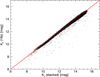 |
Fig. B.1. Comparison of KS magnitudes between the stacked and 16 s data. The red line indicates the one-to-one correlation. The shown stars have an photometric uncertainty lower than 0.05 mag. |
 |
Fig. B.2. Comparison of KS magnitudes between the stacked and 80 s data. The red line indicates the one-to-one correlation. The shown stars have a photometric uncertainty lower than 0.05 mag. |
Appendix C
Reference color correction
For the estimation of the dust extinction of a molecular cloud we need to calculate the average color of the stars behind the cloud. In order to make accurate measurements, we need to address two problems. First the cloud itself causes a strong shift of the star colors. This is exactly the effect we want to measure, but a direct measure of the color on the farther side of the cloud is impossible. Therefore, we assume the colors of stars in a nearby cloud-free region are the same as behind the cloud. Second, diffuse dust in the Milky Way causes a steady dust reddening with distance from the observer. Therefore, stars located in between the cloud and the observer will confuse the measurement of the background color and need to be removed. We address this problem by statistical subtraction of foreground stars in the JHKS color-color-space. We first bin the stars in the J–H and H–KS colors and scale the numbers with the size of the reference field, which leads to a two-dimensional histogram shown in Fig. C.1. Then, we do the same for stars located towards the highest extinction regions of the cloud. These stars are either in front of the cloud and show almost no color excess or they are behind the cloud, in which case they show a strong color excess and can be ignored. Again, we scale the number of stars per bin with the area in which they were observed. We subtract the number of stars per bin of foreground histogram from the number of stars in the corresponding bin of the reference field histogram. The resulting histogram is shown in Fig. C.2 and represents the distribution of star colors behind the cloud. Some bins show a negative number of stars, but neighboring bins show still “unreddend” stars, so they cancel in deriving the average J–H, and H–KS colors.
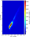 |
Fig. C.1. JHKs color–color histogram of the reference field before correction. |
 |
Fig. C.2. JHKs color–color histogram of the reference field after correction. |
Appendix D
mid-infrared near-infrared correlation
For the combination of the NIR and MIR extinction maps we convolve the MIR data (FWHM = 2.4″) to the significantly lower resolution of the NIR data (FWHM = 48″). Then, we perform a pixel-to-pixel comparison between the two maps to investigate their correlation. Figure D.1 shows only a poor correlation of the data and a large scatter. For  , the MIR extinction at most positions is underestimated by a factor of approximately five, but at some positions the data is correlated. This can be explained by the spatial filtering of the MIR mapping, which is not able to trace the diffuse cloud component. Therefore, the correlation arises only from the very inner parts of the filament. Additionally, at extinctions higher than
  , the NIR data begin to underestimate the extinction, because of a lower number of background stars in the line-of-sight. A similar behavior of the correlation can be seen in the study of Kainulainen & Tan (2013).
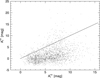 |
Fig. D.1. Pixel-to-pixel comparison of the NIR and MIR extinction values restricted to the filament area (polygon in Fig. 5). The black line indicates the one-to-one correlation. |
Appendix E
ATLASGAL clumps
Here we show cut-outs from the combined NIR and MIR extinction map of the 16 ATLASGAL GCSC sources contained in Nessie. In Sect. 4.4 we describe how these parsec-scale structures identified from ATLASGAL (white contours) break down into possibly star-forming substructures. Therefore, we show the positions of identified scale i = 2 structures with black crosses.
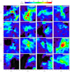 |
Fig. E.1. Half-power ellipses of 16 GCSC ATLASGAL sources (black) overlaid on combined NIR and MIR extinction maps. The crosses mark the position of substructures detected on a scale-map (s = 2) by the clumpfind-2D algorithm within the ATLASGAL sources. The white lines indicate the contours of the ATLASGAL emission. |
Appendix F
Properties of the identified structures
Here we show the properties of the identified small-scale structures, which are likely to become star formation sites. The shown properties are the results of the clumpfind-2D algorithm applied to the column density map of scale (i = 2).
Structures identified on the i = 2 scale-map.
All Tables
ATLASGAL GCSC clumps (Csengeri et al. 2014) likely embedded in the Nessie cloud.
All Figures
|
Fig. 1. NIR color-color diagram of all sources in the mapped area extracted from the VVV survey with the photometric errors lower than 0.02 mag. The blue crosses indicate non-reddened intrinsic colors of stars (Bessell & Brett 1998). The arrow shows the reddening for an extinction of AV = 10 mag. |
| In the text | |
|
Fig. 2. Extinction maps of Nessie derived using the NIR data of the VVV survey (top), MIR data of the Spitzer Space Telescope (center) and their combination (bottom). The black areas indicate regions of bright MIR emission that hampers extinction mapping. The red rectangle marks the area used for estimating the reference colors for the NICER method. The white circle marks the high-extinction region used to estimate the MIR foreground emission. |
| In the text | |
|
Fig. 3. Left: the black line shows a histogram of the calculated extinction from a high-extinction region. The red line marks the Gaussian fitted to the peak of foreground stars. Right: the black line shows the empirical weighting function, which is derived as shown in Eq. (3). The red line shows the fitted function, which is then introduced into the weighting function of the NICER method (Eq. (4)). |
| In the text | |
|
Fig. 4. Predicted stellar surface density based on the Besançon stellar distribution model (Robin et al. 2003). The blue area indicates the uncertainty arising from the scatter in the diffuse extinction measurements. The horizontal line represents the measured foreground star surface density and the vertical lines the resulting estimates of the distance and its uncertainty. |
| In the text | |
|
Fig. 5. Column density map of the Nessie filament. The white polygon marks the area chosen for the mass estimate of the cloud. The green rectangles show the positions of the zoom-ins shown in Figs. 6–8. |
| In the text | |
|
Fig. 6. Zoom-in number one of the column density map (Fig. 5). The black contours indicate the levels of 5, 10, 20, 30, 40, 50, 60 × 1021 cm−2. The white contour indicates the smoothed AV = 3 mag level. Additionally, the Class1 (“×”) and Class2 (“+”) YSOs are marked in white. |
| In the text | |
|
Fig. 7. Zoom-in number two of the column density map (Fig. 5). The black contours indicate the levels of 5, 10, 20, 30, 40, 50, 60 × 1021 cm−2. The white contour indicates the smoothed AV = 3 mag level. Additionally, the Class1 (“×”) and Class2 (“+”) YSOs are marked in white. |
| In the text | |
|
Fig. 8. Zoom-in number three of the column density map (Fig. 5). The black contours indicate the levels of 5, 10, 20, 30, 40, 50, 60 × 1021 cm−2. The white contour indicates the smoothed AV = 3 mag level. Additionally, the Class1 (“×”) and Class2 (“+”) YSOs are marked in white. |
| In the text | |
|
Fig. 9. Distributions of the separations (left) and densities (right) of the structures identified from the scale maps i = 2 (top) and i = 3 (bottom). The dashed line indicates the median and the dotted lines the 95% quantiles of each distribution. |
| In the text | |
|
Fig. 10. Median number density of structures at different spatial scales as a function of their median separation. Measurements of this study are marked with crosses. The square marks the data point derived from HNC observations of Jackson et al. (2010). The error bars show the 95% quantiles of both measurements. The blue lines indicate the scale dependency of an infinitely long cylinder in the non-turbulent case (solid), and non-thermal case (dash-dotted), and the dashed red line indicates the scale dependency of Jeans’ fragmentation. The black line shows a power-law fit to the data. |
| In the text | |
|
Fig. 11. Combined NIR and MIR extinction map (l = 338 × 10°, b = −0.45°) overlaid with the half power contour of two ATLASGAL GCSC sources (black ellipses) and their covered sources identified with clumpfind-2D from the scale 2 map. The white lines show the contours of the ATLASGAL emission. |
| In the text | |
|
Fig. 12. The H–KS vs. J–H color–color diagram for the YSO candidates in Nessie. The solid curves show the intrinsic colors for the main sequence stars (black) and giants (red; Bessell & Brett 1998), and the dash–dotted line is the locus of T Tauri stars from Meyer et al. (1997). The dashed lines show the reddening direction, and the arrow shows the reddening vector. The extinction law we adopted is from Xue et al. (2016). We note that the dashed lines separate the diagram into three regions marked with numbers 1, 2, and 3 in the figure. We use different methods to estimate the extinction of YSO candidates in different regions (see the text for details). |
| In the text | |
|
Fig. 13. The observed (left panel) and de-reddened (right panel) KS −[8.0] vs. J–H color-color diagrams for Class I+Flat (red) and Class II (green) sources in Nessie. The black arrows show the extinction vectors. |
| In the text | |
|
Fig. 14. KS absolute magnitude (MKS) histogram of Class II sources in Nessie. |
| In the text | |
|
Fig. 15. The relation between stellar mass and KS absolute magnitude of Class II sources. The black dots represent the Robitaille et al. (2006) Stage 2 models with 0.001 < Mdisk/M* < 0.01, 0.08 < M* < 7 M⊙, and 30° < inclination angle < 60°. The red curve shows the robust polynomial fitting while the gray region shows the 1σ uncertainty of the fitting. The CTTS in L1641 from Fang et al. (2013) are marked with green filled circles. Most of CTTS are located in the gray region, which confirms that this MKS − M* relation for Class II sources is consistent with the observational results. |
| In the text | |
|
Fig. 16. De-reddened luminosity functions of Class I+Flat (top panel) and Class II (bottom panel) sources in Nessie. The red vertical line shows the de-reddened luminosity completeness. |
| In the text | |
|
Fig. B.1. Comparison of KS magnitudes between the stacked and 16 s data. The red line indicates the one-to-one correlation. The shown stars have an photometric uncertainty lower than 0.05 mag. |
| In the text | |
|
Fig. B.2. Comparison of KS magnitudes between the stacked and 80 s data. The red line indicates the one-to-one correlation. The shown stars have a photometric uncertainty lower than 0.05 mag. |
| In the text | |
|
Fig. C.1. JHKs color–color histogram of the reference field before correction. |
| In the text | |
|
Fig. C.2. JHKs color–color histogram of the reference field after correction. |
| In the text | |
|
Fig. D.1. Pixel-to-pixel comparison of the NIR and MIR extinction values restricted to the filament area (polygon in Fig. 5). The black line indicates the one-to-one correlation. |
| In the text | |
|
Fig. E.1. Half-power ellipses of 16 GCSC ATLASGAL sources (black) overlaid on combined NIR and MIR extinction maps. The crosses mark the position of substructures detected on a scale-map (s = 2) by the clumpfind-2D algorithm within the ATLASGAL sources. The white lines indicate the contours of the ATLASGAL emission. |
| In the text | |
Current usage metrics show cumulative count of Article Views (full-text article views including HTML views, PDF and ePub downloads, according to the available data) and Abstracts Views on Vision4Press platform.
Data correspond to usage on the plateform after 2015. The current usage metrics is available 48-96 hours after online publication and is updated daily on week days.
Initial download of the metrics may take a while.