| Issue |
A&A
Volume 616, August 2018
|
|
|---|---|---|
| Article Number | A35 | |
| Number of page(s) | 9 | |
| Section | Astronomical instrumentation | |
| DOI | https://doi.org/10.1051/0004-6361/201731551 | |
| Published online | 10 August 2018 | |
NIKA 150 GHz polarization observations of the Crab nebula and its spectral energy distribution
1
Laboratoire de Physique Subatomique et de Cosmologie, Université Grenoble Alpes, CNRS/IN2P3,
53 avenue des Martyrs,
Grenoble,
France
2
Laboratoire Lagrange, Université Côte d’Azur, Observatoire de la Côte d’Azur, CNRS, Blvd de l’Observatoire, CS 34229,
06304
Nice cedex 4,
France
3
Institut de RadioAstronomie Millimétrique (IRAM),
Grenoble,
France
4
Laboratoire AIM, CEA/IRFU, CNRS/INSU, Université Paris Diderot, CEA-Saclay,
91191
Gif-Sur-Yvette,
France
5
Astronomy Instrumentation Group, University of Cardiff, Cardiff, Whales,
UK
6
Institut d’Astrophysique Spatiale (IAS), CNRS and Université Paris Sud,
Orsay,
France
7
Institut Néel, CNRS and Université Grenoble Alpes,
France
8
Institut de RadioAstronomie Millimétrique (IRAM),
Granada,
Spain
e-mail: This email address is being protected from spambots. You need JavaScript enabled to view it.
9
Dipartimento di Fisica, Sapienza Università di Roma,
Piazzale Aldo Moro 5,
00185
Roma,
Italy
10
Université Grenoble Alpes, CNRS, IPAG,
38000 Grenoble,
Grenoble,
France
11
Aix Marseille Université, CNRS, LAM (Laboratoire d’Astrophysique de Marseille) UMR 7326,
13388
Marseille,
France
12
School of Earth and Space Exploration, and Department of Physics, Arizona State University,
Tempe
AZ 85287,
USA
13
Université de Toulouse, UPS-OMP, Institut de Recherche en Astrophysique et Planétologie (IRAP),
Toulouse,
France
14
CNRS, IRAP,
9 Av. colonel Roche, BP 44346,
31028
Toulouse cedex 4,
France
15
University College London, Department of Physics and Astronomy,
Gower Street,
London
WC1E 6BT,
UK
16
Institut d’Astrophysique de Paris, Sorbonne Université, UPMC Univ. Paris 06, CNRS UMR 7095,
75014
Paris,
France
17
LERMA, CNRS, Observatoire de Paris,
61 avenue de l’Observatoire,
Paris,
France
18
Centro de Estudios de Física del Cosmos de Aragón (CEFCA),
Plaza San Juan, 1, planta 2,
44001
Teruel,
Spain
19
Joint ALMA Observatory & European Southern Observatory,
Alonso de Córdova 3107,
Vitacura,
Santiago,
Chile
20
Max Planck Institute for Radio Astronomy,
53111
Bonn,
Germany
21
Nordita, KTH Royal Institute of Technology and Stockholm University,
Roslagstullsbacken 23,
10691
Stockholm,
Sweden
Received:
11
July
2017
Accepted:
24
April
2018
Abstract
The Crab nebula is a supernova remnant exhibiting a highly polarized synchrotron radiation at radio and millimetre wavelengths. It is the brightest source in the microwave sky with an extension of 7 by 5 arcmin, and is commonly used as a standard candle for any experiment which aims to measure the polarization of the sky. Though its spectral energy distribution has been well characterized in total intensity, polarization data are still lacking at millimetre wavelengths. We report in this paper high resolution observations (18′′ FWHM) of the Crab nebula in total intensity and linear polarization at 150 GHz with the NIKA camera. NIKA, operated at the IRAM 30 m telescope from 2012 to 2015, is a camera made of Lumped Element Kinetic Inductance Detectors (LEKIDs) observing the sky at 150 and 260 GHz. From these observations we are able to reconstruct the spatial distribution of the polarization degree and angle of the Crab nebula, which is found to be compatible with previous observations at lower and higher frequencies. Averaging across the source and using other existing data sets we find that the Crab nebula polarization angle is consistent with being constant over a wide range of frequencies with a value of − 87.7° ± 0.3 in Galactic coordinates. We also present the first estimation of the Crab nebula spectral energy distribution polarized flux in a wide frequency range: 30–353 GHz. Assuming a single power law emission model we find that the polarization spectral index βpol = – 0.347 ± 0.026 is compatible with the intensity spectral index β = – 0.323 ± 0.001.
Key words: polarization / instrumentation: high angular resolution / instrumentation: detectors / methods: observational / supernovae: general
© ESO 2018
1 Introduction
The Crab nebula (or Tau A) is a plerion-type supernova remnant emitting a highly polarized signal (Weiler & Panagia 1978; Michel et al. 1991). Referring to Hester (2008), from inside out the Crab consists of a pulsar, the synchrotron nebula, a bright expanding shell of thermal gas, and a larger very faint freely expanding supernova remnant. Near the centre of the nebula a shock is observed; it is formed by the jet’s thermalized wind, which is confined by the thermal ejecta from the explosion (Weisskopf et al. 2000; Wiesemeyer et al. 2011). The synchrotron emission from the nebula is observed in the radio frequency domain and is powered by the pulsar located at equatorial coordinates (J2000) RA = 5h34m31.9383014s and Dec = 22°0′52.17577′′ (Lobanov et al. 2011) through its jet. The polarization of the Crab nebula radio emission, discovered in 1957 independently by Mayer et al. (1957) and Kuz’min & Udal’Tsov (1959), has confirmed that the synchrotron emission is the underlying mechanism.
Today the Crab nebula is perhaps the most observed object in the sky beyond our own solar system (Hester 2008) and often used as a calibrator by new instruments. It is also quite isolated with low background diffuse emission. In particular, it is the most intense polarized astrophysical object in the microwave sky at angular scales of a few arcminutes and for this reason it is chosen not only for high resolution cameras, but also for the calibration of cosmic microwave background (CMB) polarization experiments, which have beamwidths comparable to the extension of the source. Upcoming CMB experiments aiming at measuring the primordial B−modes require an accurate determination of the foreground emissions to the CMB signal and a high control of systematic effects. The Crab nebula has already been used for polarization cross-check analysis in the frequency range from 30 to 353 GHz (Weiland et al. 2011; Planck Collaboration XXVI 2016). High angular resolution observations from the XPOL experiment (Thum et al. 2008) at the IRAM 30 m telescope have revealed the spatial distribution of the Crab nebula in total intensity and polarization at 90 GHz with an absolute accuracy of 0.5° in the polarization angle (Aumont et al. 2010). This observation has also shown that the polarization spatial distribution varies from the source peak to the edges of the source, and illustrates the need of an accurate study at high resolution in a large frequency range to be able to use this source as a calibrator for future polarization esperiments.
Previous studies (Macías-Pérez et al. 2010) of the total spectral energy distribution (SED) have shown a spectrum well described by a single synchrotron component at radio and millimetre wavelengths, and predict negligible variations in polarization fraction andangle in the frequency range of interest for CMB studies.
Observations of the Crab nebula polarization were performed with the NIKA camera (Monfardini et al. 2010, 2014; Catalano et al. 2014)at the IRAM 30 m telescope during the observational campaign of February 2015. A first overview of the NIKA/30 m (hereafter NIKA) Crab polarization observations, focusing on instrumental characterization of the polarization system, was given in Ritacco et al. (2016). In this paper we go a step further in the analysis by combining NIKA observations with published values at other frequencies, and spanning different angular resolutions, to trace the SED in total intensity and polarization of the Crab nebula. To date, for polarization we have used observations from the WMAP satellite at 23, 33, 41, 61, and 94 GHz (Weiland et al. 2011), XPOL/30 m (hereafter XPOL) at 90 GHz (Aumont et al. 2010), POLKA/APEX (hereafter POLKA) at 345 GHz (Wiesemeyer et al. 2014), and from the Planck satellite at 30, 44, 70 (Planck Collaboration XXVI 2016), 100, 143, 217, 353 GHz to be published (Planck Collaboration III 2018).
The paper is organized as follows: in Sect. 2 the intensity and polarization maps obtained with the NIKA camera are presented together with the polarization degree and angle spatial distributions; Sect. 3 presents the reconstruction of the polarization properties of the Crab nebula in well-defined regions; Sect. 4 presents the Crab nebula SED in total intenstity and polarization; and in Sect. 5 we present our conclusions.
2 NIKA observations of the Crab nebula
2.1 NIKA camera and polarization set-up
NIKA is a dual-band camera observing the sky in total intensity and polarization at 150 and 260 GHz with 18 arcsec and 12 arcsec full width at half maximum (FWHM) resolution, respectively. It has a field of view (FoV) of 1.8′ at both wavelengths. It was operated at the IRAM 30 m telescope between 2012 and 2015. A detailed description of the NIKA camera can be found in Monfardini et al. (2010, 2011) and Catalano et al. (2014).
In addition to total power observations, NIKA was also a test bench for the polarization system of the final instrument NIKA2 (Calvo et al. 2016; Catalano et al. 2016; Adam et al. 2018), which was installed at the telescope in October 2015. The polarization set-up of NIKA consists of a continuously rotating metal mesh half-wave plate (HWP) followed by an analyser, both at room temperature and placed in front of the entrance window of the cryostat. The NIKA Lumped Elements Kinetic Inductance Detectors (LEKIDs) are not intrinsically sensitive to polarization. The HWP rotates at 2.98 Hz allowing a modulation of the polarization signal at 4 × 2.98 Hz, while the typical telescope scanning speed is equal to 26.23 arcsec s−1. These conditions provide a quasi-simultaneous measure of Stokes parameters I, Q, and U per beam and place the polarized power in the frequency domain far from the low frequency electronic noise and the atmospheric fluctuations.Ritacco et al. (2017) gives more details on the NIKA polarization capabilities and describes the performance of the instrument at the telescope. In particular the sensitivity of the NIKA camera in polarization mode was estimated to be 50 mJy.s1∕2 at 150 GHz.
NIKA has provided the first polarization observations performed with kinetic inductance detectors (KIDs), confirming that KIDs are also a suitable detector technology for the development of the next generation of polarization sensitive experiments.
2.2 NIKA observations
Observations of the polarized emission from the Crab nebula with the NIKA camera were performed at the IRAM 30 m telescope in February 2015. The average opacity at 150 GHz was τ = 0.2. Figure 1 shows the Stokes I, Q, and U maps obtained by a co-addition of 14 maps of 8 × 6 arcmin for a total observation time of ~2.4 h. The rms calculated on jack-knife noise maps is 36 mJy beam−1 on Stokes I maps and 31 mJy beam−1 on Stokes Q and U maps. The maps were performed in equatorial coordinates in four different scan directions: 0°, 90°, 120°, 150°. This allowed us to have the best mapping with different position angles.
To obtain the Stokes I, Q, and U Crab nebula maps in equatorial coordinates, we used a dedicated polarization data reduction pipeline (Ritacco et al. 2017), which is an extension of the total intensity NIKA pipeline (Catalano et al. 2014; Adam et al. 2014). The main steps of the polarization pipeline are summarized below:
- 1.
Subtraction of the HWP induced parasitic signal, which is modulated at harmonics of the HWP rotation frequency and represents the most detrimental noise contributing to the polarized signal;
- 2.
Reconstruction of the Stokes I, Q, and U time ordered information (TOI) from the raw modulated data. This is achieved using a demodulation procedure consisting in a lock-in around the fourth harmonic of the HWP rotation frequency where the polarization signal is located;
- 3.
Subtraction of the atmospheric emission in the demodulated TOIs using decorrelation algorithms. In polarization, the HWP modulation significantly reduces the atmospheric contamination and there is no need to further decorrelate the Q and U TOIs from residual atmosphere. By contrast, in intensity the atmospheric emission fully dominates the signal; to recover the large angular scales, we used the 260 GHz band as an atmosphere dominated band, as in Adam et al. (2014). This decorrelation impacts the reconstructed Stokes maps via a transfer function. We have estimated this function with simulated observations of diffuse emission that were passed through the data reduction pipeline, with the exact same scanning, sample flagging, and data processing as real data. We found that the power spectrum of the output map matches that of the input map to better than 1% (5%) on scales smaller (larger) than ~ 1′, see Fig. 2. Its moderate effect on large angular scales is further reduced with the subtraction of a zero level for the photometry (see below), so the impact of the data processing is thus negligible compared to uncertainties on absolute calibration on small scales. In the following, we therefore neglect the impact of this transfer function.
- 4.
Correction of the intensity-to-polarization leakage effect, which was identified in observations of unpolarized sourceslike the planet Uranus. For point sources the effect was about 3% peak to peak, while for extended sources like the Crab nebula it has been found to be of the order of 0.5% peak to peak. Ritacco et al. (2017) describe the algorithm of leakage correction developed specifically for NIKA polarization observations. Applying this algorithm to Uranus observations the instrumental polarization is reduced to 0.6% of the total intensity I;
- 5.
Projection of the demodulated and decorrelated Stokes I, Q, and U TOIs into Stokes I, Q, and U equatorial coordinates maps.
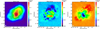 |
Fig. 1 From left to right: Crab nebula Stokes I, Q, and U maps shown here in equatorial coordinates obtained at 150 GHz with the NIKA camera. Polarization vectors, indicating both the polarization degree and the orientation, are overplotted in blue on the intensity map, where the polarization intensity satisfies |

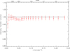 |
Fig. 2 Transfer function of the data processing in total intensity. |
2.3 Crab polarization properties
In this section we discuss the polarization properties of the source in terms of polarization degree p and angle ψ, which are defined through the Stokes parameters I, Q, and U as follows:
and
 (1)
(1)
The polarization angle follows the IAU convention, which counts east from north in the equatorial coordinate system.
These definitions are not linear in I, Q, and U, and therefore the observational uncertainties have to be carefully considered, i.e. p and ψ are noise biased. Simmons et al. (1980), Simmons & Stewart (1985) and Montier et al. (2015) proposed analytical solutions to correct for this bias. For intermediate and high signal-to-noise ratio (S/N) the polarization degree and its uncertainty read
 (2)
(2)
Furthermore, the polarization angle in a high S/N regime can be approximated by Eq. (1) with the uncertainty
 (3)
(3)
The spatial distribution map of the polarization degree p of the Crab nebula without noise bias correction is presented in the top left panel of Fig. 3. We note that we have set to 0 the pixels for which the total intensity is lower than 0.1 Jy beam−1 to avoid the divergence of p. The same has been done for the polarization angle map (bottom left of Fig. 3.)
The polarization degree p reaches a value of 20.3 ± 0.7% at the peak of the total intensity, which is consistent with what is observed in the top right panel of Fig. 3 where the variation of p as a function of the Stokes I is shown. Here the p values have been noise bias corrected and satisfy the condition  > 5
> 5  . The distribution of the polarization degree appears highly dispersed around a mean value of 20%. These points are mostly located around the peak of Stokes I. The spatial variation of p highlights the interest of high resolution polarization observations of the Crab nebula.
The bottom left panel of Fig. 3 shows the spatial distribution of polarization angle ψ. As discussed in Ritacco et al. (2017) a 1.8° uncertainty must be considered in the polarization angle coming from the determination of the HWP zero position, corresponding to its optical axis in the NIKA cabin reference frame. An uncertainty of 0.5° must be considered due to the leakage effect subtraction, which has been estimated from the comparison of the mapsbefore and after leakage correction. We observe a relatively constant polarization angle 140° < ψeq <150° represented here in equatorial coordinates, except for the north-east region where the averaged angle is around 250°, and some inner regions with lower polarization angle. These values are confirmed by the bottom right panel, which shows the polarization angle distribution as a function of total intensity satisfying the condition  .
.
The sudden change in polarization angle on the northern region was already observed by the XPOL experiment at 90 GHz (Aumont et al. 2010). This together with the variation in the polarization fraction discussed above confirms the need of high angular resolution observations at low and high frequencies for a good understanding of the Crab polarized emission properties. High resolution observations give the possibility to estimate the polarization properties at different scales and to make a comparison with low resolution experiments, for example CMB experiments.
We present in Fig. 4 the 150 GHz Crab polarization intensity map Ipol uncorrected for noise bias. We observe a peak at 0.8 Jy beam−1 and the polarization decreases towards the edges of the nebula.
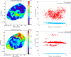 |
Fig. 3 Top left panel: polarization degree map p, uncorrected for noise bias, of the Crab nebula. Top right panel: noise bias corrected p values as a function of total intensity map (Stokes I). The condition Ipol > 5 |


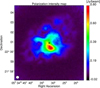 |
Fig. 4 NIKA polarized intensity map of the Crab nebula at 150 GHz. The map shows high polarized emission reaching a value of 0.8 Jy beam−1. The telescope beam FWHM is shown in the lower left. The black cross marks the pulsar position. |
2.4 Comparison to other high resolution experiments
Following previous studies, we compare here the NIKA results at the pulsar position and at Stokes I map peak with high angular resolution experiments such as POLKA, XPOL, and SCUPOL/JCMT (hereafter SCUPOL). These experiments observed at wavelengths of 870 μm, 3 mm, and 850 μm, respectively.In order to compute polarization estimates in the same region around these positions, we use POLKA (Wiesemeyer et al. 2014), XPOL (Aumont et al. 2010), SCUPOL (Matthews et al. 2009), and NIKA (this paper) maps degraded at an XPOL angular resolution of 27′′. The region is defined as an XPOL pixel size of 13.7′′.
The results obtained are shown in Table 1. The polarization degree p values are consistent for all the instruments at both positions, while for the angle ψeq we observe a fair agreement. For POLKA and SCUPOL the values found are consistent with those in Wiesemeyer et al. (2014). For XPOL the values found at the pulsar position differ from those in Aumont et al. (2010). We note that it is hard to estimate the polarization at the pulsar position precisely because it is located where the polarization changes drastically, while the peak of the total intensity is very well defined.
Polarization degree and angle estimated around the pulsar and intensity peak positions for POLKA (Wiesemeyer et al. 2014), XPOL (Aumont et al. 2010), SCUPOL (Matthews et al. 2009), and NIKA (this paper).
3 Total intensity and polarization fluxes
3.1 Total intensity flux
We computed the total flux across the Crab nebula, which has an extent of about 5′ × 7′ (see Fig. 1). We used standard aperture photometry techniques to calculate the flux as shown in the top panel of Fig. 5. We used as centre position the centre of the map with equatorial coordinates (J2000) RA = 5h 34m31.95s and Dec = 22°0′52.1′′. A zero level in the map, calculated as the mean of the signal measured on an external annular ring region (see bottom panel of Fig. 5) of radius 4.5′ < R < 5′, has been subtracted from the map. The total signal estimated is 222.7 ± 1.0 ± 1.3 ± 22.4 Jy. The first uncertainty term accounts for statistical uncertainties computed from fluctuations of the signal at large radii. The second uncertainty accounts for the difference between two sets of jack-knife noise maps. The third one accounts for the absolute calibration error of 10%. A colour correction factor of 1.05 has been accounted for. This factor was estimated using the spectral index β measured by Macías-Pérez et al. (2010) and considering the NIKA bandpass at 2 mm, as shown in Catalano et al. (2014). The final flux is thus the integrated value in the bandpass. We use Uranus for absolute point source flux calibration. The flux of the planet is estimated from a frequency dependent model of the planet brightness temperature as described in Moreno (2010). This model is integrated over the NIKA bandpasses for each channel, and it is assumed to be accurate at the 5% level. The final absolute calibration factor is obtained by fitting the amplitude of a Gaussian function of fixed angular size on the reconstructed maps of Uranus, which represents the main beam. For the polarization observational campaign of February 2015 this uncertainty is estimated to be 5% for the NIKA 2.05 mm channel (150 GHz; Ritacco et al. 2017). Nevertheless, as described in Adam et al. (2014) and Catalano et al. (2014), by integrating the Uranus flux up to 100 arcsec, we observe that the total solid angle covered by the beam is larger than the Gaussian best fit of the main beam by a factor of 28%. As a consequence we account for this factor in the estimation of the fluxes. Moreover, Adam et al. (2014) estimated the uncertainty on the solid angle of the main beam to be 4%. Finally, the overall calibration error is estimated to be about 10% by also considering the uncertainties on the side lobes.
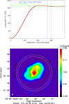 |
Fig. 5 Cumulative flux of the Crab nebula (top panel) obtained at 150 GHz over 5′ from the centre obtained by aperture photometry. The flux has been corrected by a zero level in the map, which corresponds to the mean of the signal calculated in an annular ring, as indicated by the white circles on the map and by the blue dotted lines on the top. The green dotted line represents the uncertainties measured at large radii. |
3.2 Polarization degree and angle estimates
In order to compare our results with low angular resolution CMB experiments, we present in Table 2 the integrated Stokes I, Q, and U, and the associated polarization intensity Ipol, and polarization degree p and angle ψ. A colour correction factor of 1.05 has been accounted for. All the listed values are estimated using aperture photometry inside apertures of 5′, 7′, and 9′ from the centre of the map. We limit the analysis to the maximum of the map size avoiding the edges and considering that all the flux is concentrated in 7.6′ of aperture (see Fig. 5). The uncertainties account for the calibration error of 10% discussed above. The polarization efficiency factor estimated across the NIKA 2.05 mm spectral band and reported in Ritacco et al. (2017) is ρpol = 0.9941 ± 0.0002. This very small efficiency loss of 0.6 % has a negligible impact on the estimation of the polarization fluxes and the calibration error itself. The polarization angle is presented here in equatorial coordinates and Galactic coordinates to ease the comparison with CMB experiments. The polarization angle uncertainty accounts for 2.3° systematic uncertainties, while the statistical uncertainties also accounts for Monte Carlo simulations of the noise in Q and U and the difference between two sets of jack-knife noise maps (seven maps each).
Figure 6 shows the polarization fraction (top) and polarization angle (bottom) of the Crab nebula as a function of the frequency asmeasured by five different instruments: WMAP (Weiland et al. 2011), XPOL (Aumont et al. 2010), POLKA (Wiesemeyer et al. 2014), Planck (Planck Collaboration XXVI 2016), and NIKA (this paper). We note that the WMAP satellite has FWHMs: 0.93°, 0.68°, 0.53°, 0.35°, and <0.23° at 22 GHz, 30 GHz, 40 GHz, 60 GHz, and 90 GHz, respectively. XPOL and POLKA have FWHMs of 27′′ and 20′′, respectively. The Planck satellite FWHMs are 33′, 24′, 14′, 10′, 7.1′, 5.5′, and 5′ at 30, 44, 70, 100, 143, 217, and 353 GHz, respectively. Furthermore, after discussions with the Planck team we reanalysed the Planck HFIdata using the polarization maps that will be soon published in Planck Collaboration III (2018). We have performed aperture photometry directly in the Healpix maps. The results are given in Table 3. The NIKA and POLKA values in Fig. 6 have been estimated by aperture photometry up to 9′. The XPOL value considers 10′ (Aumont et al. 2010) and the other experiments their native FWHM.
Using all the data sets and accounting for systematics as indicated in Weiland et al. (2011); Thum et al. (2008) and Rosset et al. (2010) for WMAP, XPOL and Planck respectively, we compute the weighted-average of the polarization angle ψ = − 87.7° ± 0.3°. All the observations shown on the bottom panel of Fig. 6 agree with this value within 1σ, except for POLKA. In addition we find good agreement between NIKA and POLKA and we also find that NIKA is consistent within 1σ with the Planck value at 143 GHz. The NIKA result differs from the average value by ~3°. This result could in principle be explained by an error in the calibration of the polarization angle. In Ritacco et al. (2017) a calibration angle error of 3° was also considered to explain the difference in the polarization angle of calibration sources between NIKA and the other experiments. However, the results presented in Ritacco et al. (2017) were consistent within the error bars with the other experiments and did not allow us to accurately estimate this possible shift in the angle. As NIKA is no longer in use we have no means of measuring this calibration error.
Using all the available data sets except the POLKA results, we have computed the weighted average degree of polarization and uncertanties on it. We find 6.95 ± 0.03%, as shown by the solid line and dashed lines in the top panel of Fig. 6. We observe that most of the results between 20 and 353 GHz are consistent with this value at the 1σ level, except for Planck at 70 GHz, XPOL, and POLKA, which show a significantly larger degree of polarization.
For XPOL the discrepancy can probably be explained by the lower sensitivity of the single channel XPOL experiment to the lower-than-average polarization of the outer parts of the nebula. POLKA shows a very high polarization degree due to the ~40% flux loss observed in Stokes I (see Fig. 7). This is compatible with the losses expected due to the spatial filtering of total intensity in LABOCA data reduction in this range of angular scales (Belloche et al. 2011). In the case of Planck HFI, we only find significant discrepancies for the 143 GHz data that remain unexplained to date.
The relatively constant behaviour of the polarization degree and angle over a wide frequency range suggests that the polarization emission is driven by the same physical process. We therefore expect a well-defined SED for the Crab nebula intensity and polarization emission (see next section).
NIKA Crab nebula total flux I, Q, and U, estimated by using aperture photometry methods.
Same quantities as in Table 2 derived with the new analysis of HFI Planck results by using aperture photometry of the polarization maps that will be published in Planck Collaboration III (2018).
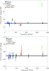 |
Fig. 6 Top panel: polarization degree as a function of frequency as measured by Planck (black dots), WMAP (blue triangles), XPOL (yellow diamond), POLKA (green cross), and NIKA (red crosses). The NIKA and POLKA values have been estimated by aperture photometry considering the source extension up to 9′. Planck and WMAP values are shown at their native resolution. XPOL, NIKA, and POLKA values have been integrated over the source. The solid line represents the weighted-averaged degree for all experiments but POLKA. Dashed lines represent 1σ uncertainties. Bottom panel: polarization angles in Galactic coordinates for the same five experiments. The solid line represents the weighted-averaged polarization angle computed using all the values. |
4 Characterization of the Crab spectral energy distribution in intensity and polarization
4.1 Intensity
The total flux density of the Crab nebula at radio and millimetre wavelengths (from 1 to 500 GHz) is mainly expected to be due to synchrotron emission and can be well described by a single power law of the form
 (4)
(4)
with spectral index β = −0.296 ± 0.006 (Baars et al. 1977; Macías-Pérez et al. 2010). Further, the emission of the Crab nebula is fading with time at a rate of α = –0.167 ± 0.015 % yr−1 (Aller & Reynolds 1985). These results suggest a low frequency emission produced by particles accelerated by the same magnetic field. Macías-Pérez et al. (2010) have also shown that there is no evidence for an extra synchrotron component or for thermal dust emission at these frequencies. The direction and degree of the polarization is therefore expected to be constant across the frequency range 30–300 GHz.
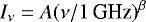
Figure 7 shows the total flux density of the Crab nebula as a function of frequency. The fluxes in the radio domain were taken from Dmitrenko et al. (1970) and Vinogradova et al. (1971). We also show microwave and millimetre wavelength fluxes from Archeops (Macías-Pérez et al. 2007), Planck (Planck Collaboration XXVI 2016), WMAP (Weiland et al. 2011), XPOL (Aumont et al. 2010), MAMBO/30 m (Bandiera et al. 2002), POLKA (Wiesemeyer et al. 2014), and GISMO/30 m (Arendt et al. 2011). The HFI Planck fluxes were specifically estimated for this paper using the new 2018 Planck HFI intensity and polarization maps, which will be made publicly available before the end of the year. We note that in these new maps the treatment of the polarization systematics has been significantly improved with respect to those in Planck Collaboration XXVI (2016). Furthermore, the Planck HFI Crab nebula fluxes in Planck Collaboration XXVI (2016) were computed assuming a point source, which is not adapted for an extended source. The measured NIKA total flux density at 150 GHz is shown in red. We note that in the plot both the best-fit model and the data represented are corrected for the fading of the source.
Assuming the single power law model in Eq. (4) and by χ2 minimization we obtain
![Mathematical equation: \[\setlength\arraycolsep{0.1em} \begin{array}{rclcl} \textrm{A}&=& 1010.2\pm3.8 & & \textrm{Jy}; \quad \quad \beta = - 0.323\pm0.001.\\ \end{array} \]](/articles/aa/full_html/2018/08/aa31551-17/aa31551-17-eq9.png)
The best-fit model is shown in Fig. 7 in cyan. The NIKA data are consistent with this model at the 1σ level. The estimated spectral index β is slightly different from the previous results provided by Macías-Pérez et al. (2010). This is probably due to the addition of new Planck and WMAP data.
As already discussed above, XPOL total power emission is low with respect to expectations. The POLKA value is found to be lower than the Planck result at the same frequency; this is mainly explained by the spatial filtering of LABOCA data reduction, as already discussed in the previous section.
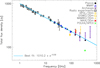 |
Fig. 7 Crab nebula total power SED as obtained from Planck (Planck Collaboration XXVI 2016) for the LFI instrument, Planck HFI data reanalysed from the maps that will be soon published in (Planck Collaboration III 2018), WMAP (Weiland et al. 2011), Archeops (Macías-Pérez et al. 2007), radio experiments (Dmitrenko et al. 1970; Vinogradova et al. 1971), XPOL/30 m (Aumont et al. 2010), NIKA/30 m (this paper), MAMBO/30 m (Bandiera et al. 2002), POLKA/APEX (Wiesemeyer et al. 2014), and GISMO/30 m (Arendt et al. 2011) data. NIKA and POLKA values are estimated over the entire extent of the source. The best-fit single power law model obtained by the analysis in this paper is shown in cyan. The best-fit models and the data both account for the Crab nebula fading with time, using 2018 as year of reference. The POLKA data flux loss (~40%) is compatible with the losses expected due to the spatial filtering of total intensity in the LABOCA data reduction (Belloche et al. 2011). |
4.2 Polarization
Though the total power emission of the Crab nebula has been monitored over decades across a wide range of frequencies, the amount of polarization data is still poor. Recent results from the Planck LFI instrument (Planck Collaboration XXVI 2016), the new Planck HFI maps presented above (Planck Collaboration III 2018), WMAP (Weiland et al. 2011), XPOL (Aumont et al. 2010), and POLKA (Wiesemeyer et al. 2014) data, together with the NIKA results allow us to trace the SED of the polarized emission, Ipol, of the Crab nebula as shown in Fig. 8. We note that the uncertainties for the NIKA polarization intensity also include absolute calibration errors and systematics as discussed in the previous sections. Assuming a single power law synchrotron emission (see Eq. (4)) for the polarization emission of the Crab nebula and a using χ2 fitting procedure we find
![Mathematical equation: \[ \setlength\arraycolsep{0.1em} \begin{array}{rclcl} \textrm{A$_{\mathrm{pol}}$}&=& 78.98\pm7.82 & & \textrm{Jy}; \quad \textrm{$\beta_{\mathrm{pol}}$} = - 0.347\pm0.026.\\ \end{array} \]](/articles/aa/full_html/2018/08/aa31551-17/aa31551-17-eq10.png)
We observe that the NIKA, XPOL, and POLKA results are consistent with the best-fit model at the 1σ level. We have also estimated the spectral index of the Crab nebula polarization emission at high frequency using the map obtained by SCUPOL (Matthews et al. 2009) at 352 GHz (850 μm) and the NIKA map. Considering only the region observed by SCUPOL (~1.5′) we obtain 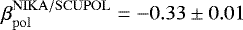 . This result is in good agreement with the best-fit model spectral index presented above.
The polarization spectral index is consistent with the total power index confirming that the synchrotron radiation is the fundamental mechanism that drives the polarization emission of the Crab nebula.
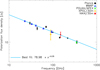 |
Fig. 8 Crab nebula polarization flux SED as obtained from Planck LFI (Planck Collaboration XXVI 2016), Planck HFI data reanalysed from the maps soon published in Planck Collaboration III (2018), WMAP (Weiland et al. 2011), XPOL (Aumont et al. 2010), POLKA (Wiesemeyer et al. 2014), and NIKA (this paper) data. NIKA and POLKA values are estimated over the entire extent of the source. The best-fit models and the data both account for the Crab nebula fading with time, using 2018 as year of reference. We also show the single power law best-fit model in cyan. |
5 Conclusions
The Crab nebula is considered a celestial standard calibrator for CMB experiments in terms of polarization degree and angle. An absolute calibration is particularly important for reliable measurements of the CMB polarization B-modes, which are a window towards the physics of the early Universe.
We have reported in this paper the first high angular resolution polarization observations of the Crab nebula at 150 GHz, which were obtained with the NIKA camera. These observations have allowed us to map the spatial distribution of the Crab nebula polarization fraction and angle.
Using the NIKA data, in addition to all the available polarization data to date, we conclude that the polarization angle of the Crab nebulais consistent with being constant with frequency, from 20 to 353 GHz, at arcmin scales with a value of − 87.7° ± 0.3 in Galactic coordinates. High resolution observations provided by NIKA at 150 GHz and POLKA at 345 GHz show a polarization angle that is lower than the average value by ~ 3° and ~ 5°, respectively. Though the uncertainties on these values are high because of the systematic errors, this discrepancy highlights the need of further high angular resolution polarization observations in this frequency range. In addition, we find a strong case for a constant polarization degree of p = 6.95 ± 0.03%.
Moreover, we have characterized the intensity and polarization SED of the Crab nebula. In both total power and polarization, we find that the data are overall consistent with a single power law spectrum, as expected from synchrotron emission from a single population of relativistic electrons.The Crab nebula presents a polarization spectral index βpol = − 0.347 ± 0.026 that is consistent with the intensity spectral index β = −0.324 ± 0.001. However, we find some discrepancies between the data sets which will require further millimetre measurements. Among future polarization experiments, NIKA2 (Calvo et al. 2016; Adam et al. 2018), will provide high sensitive polarization observations of the Crab nebula adding a 260 GHz map at 11′′ resolution.
Acknowledgements
We would like to thank the IRAM staff for their support during the NIKA campaigns. The NIKA dilution cryostat has been designed and built at the Institut Néel. In particular, we acknowledge the crucial contribution of the Cryogenics Group, and in particular Gregory Garde, Henri Rodenas, Jean Paul Leggeri, and Philippe Camus. This work has been partially funded by the Foundation Nanoscience Grenoble, the LabEx FOCUS ANR-11-LABX-0013, and the ANR under the contracts “MKIDS”, “NIKA”, and ANR-15-CE31-0017. This work has benefited from the support of the European Research Council Advanced Grant ORISTARS under the European Union’s Seventh Framework Programme (Grant Agreement no. 291294). We thank the Planck Collaboration for allowing us to use the 2018 Planck maps in advance of public release to obtain integrated flux densities in intensity and polarization in the Crab nebula. We acknowledge funding from the ENIGMASS French LabEx (R.A. and F.R.) and the CNES post-doctoral fellowship program (R.A.). We acknowledge support from the Spanish Ministerio de Economía and Competitividad (MINECO) through grant number AYA2015-66211-C2-2 (R.A.), the CNES doctoral fellowship program (A.R.), and the FOCUS French LabEx doctoral fellowship programme (A.R.). A.M. has received funding from the European Research Council (ERC) under the European Union’s Horizon 2020 research and innovation programme (Magnetic YSOs, grant agreement no. 679937).
References
- Adam, R., Comis, B., Macías-Pérez, J. F., et al. 2014, A&A, 569, A66 [NASA ADS] [CrossRef] [EDP Sciences] [Google Scholar]
- Adam, R., Adane, A., Ade, P. A. R., et al. 2018, A&A, 609, A115 [NASA ADS] [CrossRef] [EDP Sciences] [Google Scholar]
- Aller, H., & Reynolds, S. 1985, ApJ., 293, L73 [NASA ADS] [CrossRef] [Google Scholar]
- Arendt, R. G., George, J. V., Staguhn, J. G., et al. 2011, ApJ, 734, 54 [NASA ADS] [CrossRef] [Google Scholar]
- Aumont, J., Conversi, L., Thum, C., et al. 2010, A&A, 514, A70 [NASA ADS] [CrossRef] [EDP Sciences] [Google Scholar]
- Baars, J., Genzel, R., Pauliny-Toth, I., & Witzel, A. 1977, A&A, 61, 99 [NASA ADS] [Google Scholar]
- Bandiera, R., Neri, R., & Cesaroni, R. 2002, A&A, 386, 1044 [NASA ADS] [CrossRef] [EDP Sciences] [Google Scholar]
- Belloche, A., Schuller, F., Parise, B., et al. 2011, A&A, 527, A145 [NASA ADS] [CrossRef] [EDP Sciences] [Google Scholar]
- Calvo, M., Benoît, A., Catalano, A., et al. 2016, J. Low Temp. Phys., 184, 816 [NASA ADS] [CrossRef] [Google Scholar]
- Catalano, A., Calvo, M., Ponthieu, N., et al. 2014, A&A, 569, A9 [NASA ADS] [CrossRef] [EDP Sciences] [Google Scholar]
- Catalano, A., Adam, R., Ade, P., et al. 2016, ArXiv e-prints [arXiv:1605.08628] [Google Scholar]
- Dmitrenko, D., Tseitlin, N., Vinogradova, L., & Giterman, K. F. 1970, Radiophys. Quantum Electron., 13, 649 [NASA ADS] [CrossRef] [Google Scholar]
- Hester, J. J. 2008, ARA&A, 46, 127 [Google Scholar]
- Kuz’min, A. D., & Udal’Tsov, V. A. 1959, Soviet Ast., 3, 39 [NASA ADS] [Google Scholar]
- Lobanov, A. P., Horns, D., & Muxlow, T. W. B. 2011, A&A, 533, A10 [NASA ADS] [CrossRef] [EDP Sciences] [Google Scholar]
- Macías-Pérez, J., Lagache, G., Maffei, B., et al. 2007, A&A, 467, 1313 [NASA ADS] [CrossRef] [EDP Sciences] [Google Scholar]
- Macías-Pérez, J. F., Mayet, F., Aumont, J., & Désert, F.-X. 2010, ApJ, 711, 417 [NASA ADS] [CrossRef] [Google Scholar]
- Matthews, B. C., McPhee, C. A., Fissel, L. M., & Curran, R. L. 2009, ApJS, 182, 143 [NASA ADS] [CrossRef] [Google Scholar]
- Mayer, C. H., McCullough, T. P., & Sloanaker, R. M. 1957, ApJ, 126, 468 [NASA ADS] [CrossRef] [Google Scholar]
- Michel, F. C., Scowen, P. A., Dufour, R. J., & Hester, J. J. 1991, ApJ, 368, 463 [NASA ADS] [CrossRef] [Google Scholar]
- Monfardini, A., Swenson, L. J., Bideaud, A., et al. 2010, A&A, 521, A29 [NASA ADS] [CrossRef] [EDP Sciences] [Google Scholar]
- Monfardini, A., Benoit, A., Bideaud, A., et al. 2011, ApJS, 194, 24 [NASA ADS] [CrossRef] [Google Scholar]
- Monfardini, A., Adam, R., Adane, A., et al. 2014, J. Low Temp. Phys., 176, 787 [NASA ADS] [CrossRef] [Google Scholar]
- Montier, L., Plaszczynski, S., Levrier, F., et al. 2015, A&A, 574, A136 [NASA ADS] [CrossRef] [EDP Sciences] [Google Scholar]
- Moreno, R. 2010, Neptune and Uranus planetary Brightness Temperature Tabulation, Tech. rep., ESA Herschel Science Center, available from ftp://ftp.sciops.esa.int/pub/hsc-calibration/PlanetaryModels/ESA2 [Google Scholar]
- Planck Collaboration IX. 2014, A&A, 571, A9 [NASA ADS] [CrossRef] [EDP Sciences] [Google Scholar]
- Planck Collaboration XXVI. 2016, A&A, 594, A26 [NASA ADS] [CrossRef] [EDP Sciences] [Google Scholar]
- Planck Collaboration III. 2018, A&A, in press, DOI: 10.1051/0004-6361/201832909 [Google Scholar]
- Ritacco, A., Adam, R., Adane, A., et al. 2016, J. Low Temp. Phys., 184, 724 [Google Scholar]
- Ritacco, A., Ponthieu, N., Catalano, A., et al. 2017, A&A, 599, A34 [NASA ADS] [CrossRef] [EDP Sciences] [Google Scholar]
- Rosset, C., Tristram, M., Ponthieu, N., et al. 2010, A&A, 520, A13 [NASA ADS] [CrossRef] [EDP Sciences] [Google Scholar]
- Simmons, J. F. L., & Stewart, B. G. 1985, A&A, 142, 100 [NASA ADS] [Google Scholar]
- Simmons, J. F. L., Aspin, C., & Brown, J. C. 1980, A&A, 91, 97 [NASA ADS] [Google Scholar]
- Thum, C., Wiesemeyer, H., Paubert, G., Navarro, S., & Morris, D. 2008, PASP, 120, 777 [NASA ADS] [CrossRef] [Google Scholar]
- Vinogradova, L. V., Dmitrenko, D. A., & Tsejtlin, N. M. 1971, Izv. Vyssh. Uchebn. Zaved., Radiofiz., 14, 157 [NASA ADS] [Google Scholar]
- Weiland, J. L., Odegard, N., Hill, R. S., et al. 2011, ApJS, 192, 19 [Google Scholar]
- Weiler, K. W., & Panagia, N. 1978, A&A, 70, 419 [NASA ADS] [Google Scholar]
- Weisskopf, M. C., Hester, J. J., Tennant, A. F., et al. 2000, ApJ, 536, L81 [NASA ADS] [CrossRef] [PubMed] [Google Scholar]
- Wiesemeyer, H., Thum, C., Morris, D., Aumont, J., & Rosset, C. 2011, A&A, 528, A11 [NASA ADS] [CrossRef] [EDP Sciences] [Google Scholar]
- Wiesemeyer, H., Hezareh, T., Kreysa, E., et al. 2014, PASP, 126, 1027 [NASA ADS] [CrossRef] [Google Scholar]
All Tables
Polarization degree and angle estimated around the pulsar and intensity peak positions for POLKA (Wiesemeyer et al. 2014), XPOL (Aumont et al. 2010), SCUPOL (Matthews et al. 2009), and NIKA (this paper).
NIKA Crab nebula total flux I, Q, and U, estimated by using aperture photometry methods.
Same quantities as in Table 2 derived with the new analysis of HFI Planck results by using aperture photometry of the polarization maps that will be published in Planck Collaboration III (2018).
All Figures
|
Fig. 1 From left to right: Crab nebula Stokes I, Q, and U maps shown here in equatorial coordinates obtained at 150 GHz with the NIKA camera. Polarization vectors, indicating both the polarization degree and the orientation, are overplotted in blue on the intensity map, where the polarization intensity satisfies |
| In the text | |
|
Fig. 2 Transfer function of the data processing in total intensity. |
| In the text | |
|
Fig. 3 Top left panel: polarization degree map p, uncorrected for noise bias, of the Crab nebula. Top right panel: noise bias corrected p values as a function of total intensity map (Stokes I). The condition Ipol > 5 |
| In the text | |
|
Fig. 4 NIKA polarized intensity map of the Crab nebula at 150 GHz. The map shows high polarized emission reaching a value of 0.8 Jy beam−1. The telescope beam FWHM is shown in the lower left. The black cross marks the pulsar position. |
| In the text | |
|
Fig. 5 Cumulative flux of the Crab nebula (top panel) obtained at 150 GHz over 5′ from the centre obtained by aperture photometry. The flux has been corrected by a zero level in the map, which corresponds to the mean of the signal calculated in an annular ring, as indicated by the white circles on the map and by the blue dotted lines on the top. The green dotted line represents the uncertainties measured at large radii. |
| In the text | |
|
Fig. 6 Top panel: polarization degree as a function of frequency as measured by Planck (black dots), WMAP (blue triangles), XPOL (yellow diamond), POLKA (green cross), and NIKA (red crosses). The NIKA and POLKA values have been estimated by aperture photometry considering the source extension up to 9′. Planck and WMAP values are shown at their native resolution. XPOL, NIKA, and POLKA values have been integrated over the source. The solid line represents the weighted-averaged degree for all experiments but POLKA. Dashed lines represent 1σ uncertainties. Bottom panel: polarization angles in Galactic coordinates for the same five experiments. The solid line represents the weighted-averaged polarization angle computed using all the values. |
| In the text | |
|
Fig. 7 Crab nebula total power SED as obtained from Planck (Planck Collaboration XXVI 2016) for the LFI instrument, Planck HFI data reanalysed from the maps that will be soon published in (Planck Collaboration III 2018), WMAP (Weiland et al. 2011), Archeops (Macías-Pérez et al. 2007), radio experiments (Dmitrenko et al. 1970; Vinogradova et al. 1971), XPOL/30 m (Aumont et al. 2010), NIKA/30 m (this paper), MAMBO/30 m (Bandiera et al. 2002), POLKA/APEX (Wiesemeyer et al. 2014), and GISMO/30 m (Arendt et al. 2011) data. NIKA and POLKA values are estimated over the entire extent of the source. The best-fit single power law model obtained by the analysis in this paper is shown in cyan. The best-fit models and the data both account for the Crab nebula fading with time, using 2018 as year of reference. The POLKA data flux loss (~40%) is compatible with the losses expected due to the spatial filtering of total intensity in the LABOCA data reduction (Belloche et al. 2011). |
| In the text | |
|
Fig. 8 Crab nebula polarization flux SED as obtained from Planck LFI (Planck Collaboration XXVI 2016), Planck HFI data reanalysed from the maps soon published in Planck Collaboration III (2018), WMAP (Weiland et al. 2011), XPOL (Aumont et al. 2010), POLKA (Wiesemeyer et al. 2014), and NIKA (this paper) data. NIKA and POLKA values are estimated over the entire extent of the source. The best-fit models and the data both account for the Crab nebula fading with time, using 2018 as year of reference. We also show the single power law best-fit model in cyan. |
| In the text | |
Current usage metrics show cumulative count of Article Views (full-text article views including HTML views, PDF and ePub downloads, according to the available data) and Abstracts Views on Vision4Press platform.
Data correspond to usage on the plateform after 2015. The current usage metrics is available 48-96 hours after online publication and is updated daily on week days.
Initial download of the metrics may take a while.