| Issue |
A&A
Volume 615, July 2018
|
|
|---|---|---|
| Article Number | A116 | |
| Number of page(s) | 14 | |
| Section | Stellar structure and evolution | |
| DOI | https://doi.org/10.1051/0004-6361/201732542 | |
| Published online | 24 July 2018 | |
Evolution of the magnetic field of Betelgeuse from 2009–2017★
1
IRAP, Université de Toulouse, CNRS, UPS, CNES,
57 avenue d’Azereix,
65000
Tarbes, France
e-mail: This email address is being protected from spambots. You need JavaScript enabled to view it.
2
IRAP, Université de Toulouse, CNRS, UPS, CNES,
14 Avenue Edouard Belin,
31400
Toulouse, France
3
Université de Montpellier, CNRS, LUPM,
Place Eugène Bataillon,
34095
Montpellier, France
4
Dunlap Institute for Astronomy and Astrophysics, University of Toronto,
Rm 101, 50 St. George Street,
Toronto
ON
M5S 3H4, Canada
5
Laboratoire d’Astrophysique de Bordeaux, Univ. Bordeaux, CNRS, B18N,
Allée Geoffroy Saint-Hilaire,
33615
Pessac, France
6
Université Côte d’Azur, Observatoire de la Côte d’Azur, CNRS, Lagrange, CS 34229,
06304
Nice Cedex 4, France
7
Institute of Astronomy, KU Leuven,
Celestijnenlaan 200D B2401,
3001
Leuven, Belgium
8
Institute of Astronomy and NAO, Bulgarian Academy of Sciences,
72 Tsarigradsko shose,
1784
Sofia, Bulgaria
9
LESIA, Observatoire de Paris, PSL Research University, CNRS, UPMC, Univ. Paris-Diderot,
5 place Jules Janssen,
92195
Meudon, France
10
Department of Physics, Royal Military College of Canada,
PO Box 17000, Station Forces,
Kingston
ON
K7K 4B4, Canada
Received:
23
December
2017
Accepted:
5
March
2018
Abstract
Context. Betelgeuse is an M-type supergiant that presents a circularly polarized (Stokes V) signal in its line profiles, interpreted in terms of a surface magnetic field.
Aims. The weak circular polarization signal has been monitored over 7.5 years in order to follow its evolution on different timescales, and eventually to determine its physical origin. Linear polarization measurements have also been obtained regularly in the last few years.
Methods. We used both the ESPaDOnS and Narval spectropolarimeters to obtain high signal-to-noise ratio spectra, which were processed by means of the least-squares deconvolution method. In order to ensure the reality of the very weak circular polarization, special care has been taken to limit instrumental effects. In addition, several tests were performed on the Stokes V signal to establish its stellar and Zeeman origin.
Results. We confirm the magnetic nature of the circular polarization, pointing to a surface magnetic field of the order of 1 G. The Stokes V profiles present variations over different timescales, the most prominent one being close to the long secondary period (LSP; around 2000 d for Betelgeuse) often invoked in red evolved stars. This long period is also dominant for all the other Stokes parameters. The circular polarization is tentatively modeled by means of magnetic field concentrations mimicking spots, showing in particular that the velocity associated with each “spot” also follows the long timescale, and that this signal is nearly always slightly redshifted.
Conclusions. From the coupled variations of both linear and circular polarization signatures in amplitude, velocity and timescale, we favour giant convection cells as the main engine at the origin of polarization signatures and variations in all the Stokes parameters. This strengthens support for the hypothesis that large convective cells are at the origin of the LSP.
Key words: stars: magnetic field / stars: individual: Betelgeuse / stars: late-type / supergiants
Based on observations obtained at the Télescope Bernard Lyot (TBL) at Observatoire du Pic du Midi, CNRS/INSU and Université de Toulouse, France, and at the Canada-France-Hawaii Telescope (CFHT) which is operated by the National Research Council of Canada, CNRS/INSU and the University of Hawaii.
© ESO 2018
 Open Access article, published by EDP Sciences, under the terms of the Creative Commons Attribution License (http://creativecommons.org/licenses/by/4.0;), which permits unrestricted use, distribution, and reproduction in any medium, provided the original work is properly cited.
1 Introduction
Cool evolved stars play a major role in the enrichment of the interstellar medium through their strong winds. However, the mechanisms that drive mass loss from these stars are not well understood. Mechanisms that are often invoked include thermal gas and radiation pressure, acoustic and shock waves, Alfvén waves, magnetism, and most probably other additional phenomena. Magnetism is one of these factors, and in this context, dedicated spectropolarimetric studies of cool evolved stars have been undertaken. Recent examples include the Mira variable star χ Cyg (Lèbre et al. 2014), the radially pulsating RV Tauri stars (Sabin et al. 2015), some red giants (Aurière et al. 2015) as well as FGK supergiants (Grunhut et al. 2010) which suggest that magnetic fields may well be present in all cool, evolved stars.
One of the first detections of the magnetic field of a red supergiant (RSG) concerned Betelgeuse: using the Narval spectropolarimeter, Aurière et al. (2010) detected a weak circular polarization Stokes V signal. From the complex behavior of the Stokes V profile, and using the center of gravity technique (Rees & Semel 1979), the longitudinal magnetic field integrated over the stellar disk was estimated to be of the order of 1 G (Aurière et al. 2010). In addition, it was also noted (Petit et al. 2013) that the double-peaked Stokes V profiles of Betelgeuse all possess a significant level of asymmetry, and are additionally red-shifted by about 9 km s−1 with respect to the Stokes I profiles. Finally, a recent study (Tessore et al. 2017) also reports the magnetism of two other RSGs, CE Tau and μ Cep, which also present complex structures within their Stokes V signal.
The distorted Stokes V signatures often observed in RSGs suggest topologically complex magnetic fields, presumably generated by dynamo action. The engine would be related to either giant cells (Stothers & Leung 1971) or to the supergranulation cells of Schwarzschild (1975). These gigantic convection cells have been reproduced through numerical simulations (e.g., Freytag et al. 2002; Chiavassa et al. 2011a) and directly seen in spatially resolved observations of for example, Betelgeuse (Haubois et al. 2009). These flows of plasma could then create global and local magnetic fields in RSGs (Dorch & Freytag 2003).
Generally speaking, atmospheric motions in RSGs are difficult to understand (e.g., Josselin & Plez 2007), and this complex velocity field is probably the main cause of line profile broadening, of the order of 20 km s−1. In addition, RSGs often show complex photometric and spectroscopic variability on several timescales, ranging from hundreds to thousands days (e.g., Percy & Kathu 2014). In particular, Betelgeuse has at least two photometric timescales, a “short” one, of the order of 400 d, and a longer one, often called the long secondary period (LSP), of the order of 2000 d (Kiss et al. 2006).
In order to extend the pioneering study of Aurière et al. (2010), dedicated to the first detection and the study of the magnetic field at the surface of Betelgeuse, we undertook a (still ongoing) spectropolarimetric follow-up of Betelgeuse. Stokes V observationsare described in Sect. 2, and their stellar origin is established in Sect. 3. The V signal is then analyzed in terms of magnetic field in Sect. 4. A rough frequency analysis of the variations of the Stokes parameters is presented in Sect. 5. Then, an attempt to model the Stokes parameters in terms of bright spots and magnetic concentrations is described in Sect. 6. Finally, some concluding remarks are discussed in Sect. 7.
2 Observations with Narval and ESPaDOnS
We carried out long-term spectropolarimetric monitoring of Betelgeuse from September 2009 to April 2017 using Narval (Aurière 2003) and ESPaDOnS (Donati et al. 2006), representing eight seasons of data acquired on 76 dates. We note that from November 2013, linear polarization Stokes Q and U observations have also been obtained, with Narval only, quasi-simultaneously with each Stokes V series. All spectra have a resolving power of 65 000 and cover the wavelength range 370–1048 nm.
A standard polarization observation consists of a series of 4 sub-exposures, following the procedure described by Semel et al. (1993). To avoid saturation of the CCD detector, we performed very short exposures (3–5 s for Narval, depending on sky quality, and 1 s for ESPaDOnS, for each sub-exposure). We obtained around ten Stokes V∕Ic series per observing night, which are averaged. For the Stokes parameters Q∕Ic and U∕Ic obtained with Narval, because the signal amplitude is larger by a factor of about ten compared to the Stokes V , the number of exposures was reduced. Also included in the measurements are the “diagnostic null” spectra N1,2 obtained from different combinations of the four sub-exposures. These spectra are in principle featureless, and are used to diagnose the potential presence of spurious contributions to the Stokes V spectrum. Each single spectrum used in this work has a peak signal-to-noise ratio (S/N) ranging from 1700 to 2100 in Stokes I (per 1.8 km s−1 spectral bin). Details of the observing and reduction procedure are described by Donati et al. (1997), Aurière et al. (2009, 2016). We note here that all spectra presented in the different figures in this paper have been smoothed for clarity using a moving average over three pixels; the analysis was however performed using unsmoothed data. Table A.1 presents the journal of observations giving the date and heliocentric Julian day corresponding to mid-observation, the instrument (N for Narval, E for ESPaDOnS), the number of Stokes V spectra collected on the given night, a unique label used to indicate each night (or the average over several close nights), and the season number (starting from autumn 2009), defined as the epoch when Betelgeuse is observable (typically September–April). Table 1 is the journal of the Stokes Q and U observations, extending the initial monitoring already presented in Aurière et al. (2016), giving the date of the observation night as well as the characteristics of the spots (Sect. 6, see also Aurière et al. 2016). To obtain a high-precision diagnosis of the spectral line polarization, the least-squares deconvolution method (LSD, Donati et al. 1997) was applied to each reduced Stokes I, Q, U, and V spectrum. We used a solar abundance line mask (similar to that of Aurière et al. 2016), calculated from data provided by VALD (Kupka et al. 1999) for an effective temperature of 3750 K, log g = 0.0, and a microturbulence of 4.0 km s−1, consistent with the physical parameters of Betelgeuse (Josselin & Plez 2007; Lambert et al. 1984). The mask contains about 15 000 atomic lines with a depth larger than 40% of the continuum. Application of LSD using this mask allows the detection of clear polarisation structures in the LSD profiles that are discussed below.
3 The stellar origin of the Stokes V signal
A spectropolarimetric survey of supergiants performed with ESPaDOnS (Grunhut et al. 2010) obtained a marginal detection for Betelgeuse. This marginal detection was immediately confirmed by Aurière et al. (2010) who detected the magnetic field of Betelgeuse during the spring of 2010 using the Narval spectropolarimeter. As described in Sect. 2, in order to obtain a high-precision diagnosis from the Stokes parameters, both teams used the LSD method (Donati et al. 1997). Aurière et al. (2010) give arguments showing that the detected Stokes V signal is not spurious. Since this discovery, Betelgeuse has been followed up during each visibility season with Narval or ESPaDOnS. The Stokes V parameter is found to have a variable amplitude and shape, with a strength remaining at the level of a few times 10−5 of the unpolarized continuum. However, the null polarization signals N1,2 sometimes present features that can potentially be diagnostics of problems with the circular polarization analysis. Moreover, since linear polarization (which is about ten times larger than the circular polarization for Betelgeuse) has been detected (Aurière et al. 2016), it may also lead to crosstalk into the Stokes V spectra (as shown by Tessore et al. 2017), again preventing a clear interpretation of this latter signal.
Therefore, the reality of the V signal should first be carefully evaluated in order to interpret our relatively low-amplitude signal as a time series. It should be pointed out that, while the Zeeman signature of Betelgeuse is weak, weaker magnetic detections have been obtained both in cool and tepid bright stars, for example, other supergiants (Grunhut et al. 2010), red giants (Pollux, Aldebaran, Arcturus and Alphard; Aurière et al. 2015), and the A-type stars Vega (Lignières et al. 2009), Sirius (Petit et al. 2011), β Leo, and θ Leo (Blazère et al. 2016). For all these detections, the polarization origin of the Stokes V signal has been evaluated, and a Zeeman origin is the most likely hypothesis. More recently, Tessore et al. (2017) have detected magnetic fields at the surface of two RSGs (CE Tau and μ Cep), and clarified the nature of the spurious N signal that can appear in observations of RSGs.
3.1 Influence of crosstalk on Stokes V measurements
The twin spectropolarimeters ESPaDOnS and Narval experience reciprocal crosstalk between linear and circular polarization which must be taken into account when investigating very small linear polarization levels in the presence of very high circular polarization signals, and vice versa (e.g., Silvester et al. 2012). Since linear polarization has been detected in the spectral lines of Betelgeuse (Aurière et al. 2016), it is important to further study the crosstalk from (strong) linear to (weak) circular polarization signals.
In the case of ESPaDOnS, a deep investigation of the crosstalk problem was carried out, and the crosstalk was ultimately reduced below the 1% level at the time of our observations (Barrick et al. 2010; Silvester et al. 2012), namely at 0.5% or lower for both Stokes Q or U to Stokes V .
The crosstalk of Narval has been measured directly on the sky by observing the (strongly) magnetic Ap star γ Equ. In September 2009 (Silvester et al. 2012), it was found to be 3.1% from Stokes V to Stokes Q and below 0.2% from Stokes V to Stokes U, the process being supposed to be reciprocal (and assuming no crosstalk between Q and U). In September 2016, the same test provided values of 1% and 1.5% respectively. Thus, crosstalk of Narval from Q to V and U to V , assuming that it is reciprocal, is at most of the order of a few percent (3%).
Recent Narval observations of the RSG μ Cep by Tessore et al. (2017) show that this star presents, as does Betelgeuse, a much more important linear polarization signal than circular polarization. From a dedicated observational procedure performed with Narval, these authors are able to disentangle and model the crosstalk. For Q to V and U to V , they obtained respectively 3.6% and 1.4%, a result consistent with that obtained above for the Ap star, and that confirms the reciprocity between linear and circular polarization signals.
For Betelgeuse, Stokes Q and U observations with Narval present signals up to the 7–9 × 10⁻⁴ level, especially in 2014 (Aurière et al. 2016). This level of linear polarization would lead to a crosstalk with ESPaDOnS of about 2 × 10⁻⁶, that is three times smaller than the signal observed on February 14, 2012, when the Stokes V signal amplitude was about 6 × 10⁻⁵ (Fig. 1). Therefore, this ESPaDOnS observation is effectively crosstalk-free. Comparing with the Narval observation of Betelgeuse obtained a few nights earlier (i.e., well below the expected variation timescale, see Sect. 5), on February 10, 2012, also presented in Fig. 1, it is clear that both Stokes V profiles have the same amplitude. This demonstrates that on February 10, 2012, the crosstalk of Narval did not significantly affect the Stokes V signals. Generally speaking, in the case of Narval, the crosstalk from the maximum observed linear polarization would be less than 2 × 10⁻⁵.
To generalize the weak influence of the crosstalk on the whole data set, we take advantage of our quasi-simultaneous Stokes QUV Narval observations. When both linear and circular polarization measurements were obtained within a two-day interval (corresponding to 17 sequences), we compared the extrema of the different signals. It appears, from the analysis of these 17 QUV sequences, that the V signal amounts to between 4.5% and 38% of the linear polarization, being 12% on average – much larger than the expected crosstalk contribution. Figure 2 presents the measurements of QUV signals for two nights, with the V profile enhanced by a factor of ten with respect to the QU profiles. A first remark is that the N1 signal is flat for all Stokes parameters. On November 27, 2013, the weak positive peak of Stokes V at about 20 km s−1 is not aligned withany QU peaks (whatever their sign), and the aligned linear (absolute) value leads to V∕Q or V∕U of about 10% – well above the 3% crosstalk limit. The situation is the same for the night of April 8, 2014, where all the peaks, aligned within a few km s−1, show circular to linear ratios again of the order of 10%. In addition, for both nights, the V signal presents a structure located at a velocity of about 50 km s−1 that is not present at all in the QU signals (possibly even extending outside the I profile), and thus it cannot be attributed to a crosstalk effect from QU to V . Hence, we conclude that the detectedStokes V signal is not due to, and only marginally affected by, crosstalk from the Stokes Q and U signals.
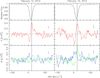 |
Fig. 1 Stokes I, Stokes V , and null polarization N1 (blue) and N2 (green) LSD profiles of Betelgeuse for February 14 (ESPaDOnS) and 10 (Narval), 2012. Small vertical lines represent typical error bars. The vertical line corresponds to the heliocentric radial velocity (HRV) of Betelgeuse (about 21 km s−1). |
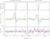 |
Fig. 2 IQUV LSD profiles of Betelgeuse for 27 November 2013 and April 8, 2014. Top panel: Stokes I. Middle panel: Stokes Q (blue), U (red), and V (green) signals, where the V signal has been magnified by a factor ten. Bottom panel: null polarization signal N1 , with the same color code as for the Stokes parameters. Small vertical lines represent typical error bars with the same color code. The vertical line corresponds to the HRV of Betelgeuse (about 21 km s−1). |
3.2 Null polarization N1,2 signatures associated with Stokes V profiles of Betelgeuse
In addition to the QUV parameters, the LSD procedure provides two null polarization signals N1 and N2 (see Donati et al. 1997). These profiles are used to diagnose spurious contributions to the polarization, in particular for weak Stokes V profiles suchas those of Betelgeuse. In principle they should be featureless, but we in fact observe nonzero signatures in some of the N spectra associated with our observations. This is not uncommon, and can have a variety of explanations. For example, stellar variability or changing sky conditions during the four sub-exposures may induce a spurious signal in N. In addition, Folsom et al. (2016) found that for young cool stars, in the case of poor S/N, an nonzero N signal couldoccur due to the very noisy blue part of the spectrum. This appears to be partly the case for ournoisiest spectra, but even removing their bluest parts does not appreciably clean the N1,2 signals. Betelgeuse is not a rapidly varying star and we managed to observe it in good atmospheric conditions in order to detect the very weak Stokes V signal (~ 1–2 × 10⁻⁵). The detection of N signatures is therefore something of a puzzle.
From the two close nights of February 2012 presented in Fig. 1, it is shown that while the ESPaDOnS N1,2 spectra are similar and unambiguously weaker than the V signal, the corresponding Narval data present structures within both N1,2 spectra thathave amplitudes close to the circular polarization signal. However, we note that both Stokes V shapes are comparable for both considered nights, separated by less than four nights, that is, well below the expected timescale for variation of the polarimetric signal (see Sect. 5). Hence, since the Narval observation shows strong null polarization signals while the ESPaDOnS observation does not, we can infer that the N behavior does not significantly alter Narval’s Stokes V signal.
The occurrence of significant N1,2 signals in observations of Betelgeuse, both with Narval and ESPaDOnS (and also observed by Grunhut et al. 2010) is more frequent than in any other star observed so far, apart from the RSG star μ Cep (Tessore et al. 2017). These authors have shown that in the case of μ Cep, when disentangling Zeeman and crosstalk contributions to Stokes V , the main part of the N1,2 signals was contaminated by the linear polarization. Looking closely at the observations of the magnetic Ap star γ Equ, which enables the disentangling of Zeeman and crosstalk contributions to Stokes Q and U, we found the same effect: the N1,2 profiles corresponding to both Stokes Q and U measurements can be obviously polluted by the strong Stokes V signal at the 10−2 level. As an example for Betelgeuse, Fig. 3 presents, for two nights for which both linear and circular measurements have been obtained, the null N1,2 signals of the V measurements together with the linear polarization Q and U signals. For both nights, at least one N signal (multiplied by a factor of −20 for illustrative purposes) is very similar to the U profile, and to a lesser extent, to the Q profile. An interesting observation is that while N2 mimics the Q, U signals on the night April 8, 2014, it is the N1 profile that is affected on the night of December 18, 2014. Therefore, it appears that the N measurements are affected by the strong linear polarization in various ways. In particular, the N profiles may reflect the linear polarization by an amount estimated to be of about 2.5%. Thus, structures present within the N signals that are below 2.5% of the QU polarization amplitudes for a given wavelength may not be attributed to spurious extra-contributions.
Therefore, in order to restrict our analysis to what we presume to be the most reliable data, we decided to remove observations(i.e., the corresponding nights) that exhibit large and/or structured null polarization profiles. This represents a relaxation of the criterion proposed by Bagnulo et al. (2009) who suggested to reject all profiles with corresponding N signal above the 3σ level. The retained data are provided in Table A.1 when the column “label” contains an entry. Therefore, most of the data in Table A.1 will be used for the work on Stokes I profiles (Mathias et al., in prep.), but our results on Stokes V profiles will only be based on spectra with N1,2 profiles presenting signals significantly weaker than the corresponding circular polarization signals, which represents 30 epochs. The 30 LSD profiles for Stokes I, V and N1,2 are illustrated in Fig. 4. We note that a three-pixel filtering is performed on the profiles to enhance visibility of the signal with respect to the noise.
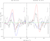 |
Fig. 3 StokesQ (blue), U (red), and from the V measurements N1 (continuous)and N2 (dashed) LSD profiles of Betelgeuse for April 08, 2014 (left) and December 18, 2014 (right) obtained with Narval. Small vertical lines represent typical error bars with the same color code. We note that the N1,2 signals have been multiplied by a factor −20. |
4 Properties of the Zeeman signal
4.1 Evaluating the Zeeman origin of Stokes V
Since magnetic fields have already been detected in a large number of cool and evolved stars through spectropolarimetric observations (see Sect. 1), it is very likely that the circular polarization detected in Betelgeuse is due to the Zeeman effect as well. The general shape of the Stokes V signal (e.g., in observation N20111208) is actually reminiscent of that predicted by the Zeeman effect (Mathys 1993) in the case of a single spot with homogeneous velocity and magnetic field. However, since the level of the signal is very weak, following Blazère et al. (2016), we performed different tests to ascertain the Zeeman nature of the Stokes V signal, by comparing different LSD profiles computed from selected masks. Indeed, in the first order approximation, valid for weak fields and safely applicable to most cool stars, Stokes V is proportional to the derivative of the intensity with respect to the velocity d I∕d v (i.e., the depth), to the wavelength, and to the effective Landé factor geff. We note that this approximation may be insufficient in some cases, for instance for profiles distorted by a complex velocity field.
For a star with negligible rotational broadening of its spectral lines, the “classical” Zeeman picture predicts that lobes of positive and negative signs should be observed, resulting in the well-known characteristic S shape of the V signal. A few nights that present suchan unambiguous S shape were selected, and we performed tests in particular according to the proportionality of the V signal with the Landé factor, which quantifies the magnetic sensitivity. The complete mask described in Sect. 2 was split into two sub-masks (about 6000 lines each) of low and high Landé factors, the separation being at geff = 1.207 as an average of the whole mask. The resulting LSD profile was then normalized in order to obtain the same Stokes I profile depth. Since the Stokes V signal is weak in the case of Betelgeuse, the tests were compared to an M giant star for which a magnetic field (of about 5 G) has been confidently detected, EK Boo (Konstantinova-Antova et al. 2010). Figure 5 displays a representative example of this comparison. As expected for a Zeeman effect, we note a clear increase of the Stokes V signal for the high-Landé sub-mask (⟨geff⟩ = 1.425) compared to the low-Landé mask (⟨geff⟩ = 0.878).
Such tests have also been performed for the two other parameters: line depth and wavelength. In the first case, the sub-masks also confirm the Zeeman effect, but the increase of the signal with line depth is not a unique characteristic of Zeeman effect, as it is also observed in the case of scattering processes (Aurière et al. 2016). As for the second case, because of the low temperatureof the star, LSD profiles computed from the blue sub-mask were very noisy and did not lead to convincing results.
4.2 Zeeman polarity and crossover profiles
Interpreting our Stokes V signals as due to Zeeman effect in the case of weak magnetic fields enables us to study their S shape (Mathys 1989, 1993) and to infer their polarity. In this work, the positive Stokes V polarity corresponds to a positive first (blue) lobe; the negative Stokes V polarity corresponds to a negative first (blue) lobe. We see in Fig. 4 that the polarity changes between positive (e.g., N20100300, N20130908) and negative (e.g., N20111008). In addition, configurations similar to crossover effect (composition of two opposite polarity signals, Babcock 1951) also occur (e.g., E20101121, N20110205, E20121000). Furthermore, the peculiar shape of the detected crossovers is observed at the required time of the polarity change: the Stokes V profile is symmetrical with respect to the radial velocity inferred from the I profile. However, if the Stokes V profile shape may be more or less interpreted in terms of a classical Zeeman signal until 2014, the situation becomes unclear after that date as many V signatures (e.g., N20160912, N20161203) present nonstandard structures.
A summary of the interpretation of the V measurements is represented in Fig. 6. The polarization has changed at least three times between March 2010 and April 2014. During these five seasons the Stokes V signal mainly presents two lobes, as in the classical Zeeman shape. The crossover profile itself has occurred three times during these five observing seasons, twice in the 2010/2011 season (Season 2) and once in 2012 (Season 4). During the three next seasons (Seasons 6–8) the shape of the Stokes V profile is more ambiguous: except for December 2014 and January 2015 when a positive polarity clearly appears, the shape of the Stokes V profile is much more complex.
4.3 The longitudinal magnetic field Bℓ
The surface-averaged longitudinal magnetic field Bℓ may be computed from the V signal using the first-order moment method (Rees & Semel 1979), adapted to LSD profiles (Donati et al. 1997; Wade et al. 2000). However, this method assumes that Stokes I and V share a common center of gravity, which is usually not the case for Betelgeuse, since the polarization signal is found to be redshifted (Petit et al. 2013, see also Sect. 6). In addition, the I signal is asymmetric, its shape being modified in particular by the convective velocity field (Josselin & Plez 2007, Mathias et al., in prep.). Finally, and especially during Seasons 6–8, the shape of Stokes V is very complex and cannot be assimilated to a profile having unambiguous parameters on the stellar surface, meaning one not characterized through a single location and/or field intensity. Therefore, the “classical” (i.e., first-order moment) measurements of Bℓ can only provide an estimate of the magnitude of an averaged longitudinal magnetic field, having a value around 1 G. The Bℓ measurements obtained using the first-order moment method are illustrated in Fig. 7. This complements the work presented by Bedecarrax et al. (2013, their Fig. 1). We underscore the fact that the interpretation of these measurements is not as straightforward as in stars having a localized magnetic field such as Ap stars, see Sects. 6 and 7.
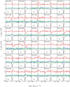 |
Fig. 4 StokesV (red), null polarization N1 (blue) and N2 (green), and I (black) LSD profiles of Betelgeuse for the 30 dates selected as described in Sect. 3.2and spanning along the eight seasons between March 2010 and April 2017 (Table A.1). We note that the UT observation date is encoded for each retained night (see Table A.1). The vertical line corresponds to the HRV of Betelgeuse (about 21 km s−1). |
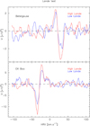 |
Fig. 5 Comparison of Stokes V profiles obtained by selecting photospheric lines of low (blue line) and high (red line) magnetic sensitivity according to the Landé factor. Top panel: Betelgeuse on December 9, 2010. Bottom panel: the magnetic M giant EK Boo on March 18, 2009. |
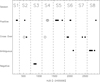 |
Fig. 6 Variations of polarity during the eight observation seasons 2010–2017 (S1–S8). Open and full symbols represent ESPaDOnS and Narval, respectively. |
5 Timescales of variation of the Stokes parameters
Red supergiants often present semi-regular variations that have been attributed to radial stellar pulsations (e.g., Stothers 1972) and/or to largescale convection in the envelope (e.g., Stothers 2010). For Betelgeuse, many attempts to derive periods have been carried out; the most extensive of which is that of Kiss et al. (2006) who analyzed an extended data set from the AAVSO photometric database. This latter study shows that, as other RSGs,Betelgeuse presents two variation timescales: a relatively fast one, of the order of 400 d, that can be attributed to a fundamentalor low-order overtone radial mode, and a relatively slow one, of the order of 2000 d, often referred to as the LSP. These LSPs, well known in the less-massive AGB stars, are still poorly understood. Common interpretations involve binarity, nonradial g-modes or magnetic activity (Wood et al. 2004).
From Fig. 6, we see that polarity changes occur with timescales ranging from about 3 months (between the two crossover phases observed in 2010) to about two years, between October 2012 and September 2014 (hypothesing that there is no rapid change of polarity between the observing seasons). While these changes appear very clearly during Seasons 1–5, the polarity of the Stokes V parameter is more challenging to determine for Seasons 6–8. It may be thus interesting to investigate if a polarity change timescale is present or not, and if this timescale can help to understand the origin of the V signal variations. So, despite our relatively short dataset for the Stokes V measurements (about 7.5 years), we attempted a frequency analysis.
We thus considered the data set corresponding to the 30 retained nights (see Table A.1) and we proceeded to apply a standard 2D Fourier analysis (CLEAN, Roberts et al. 1987) up to a frequency f = 0.01 d−1. Results are presented in Fig. 8. Signal is present in three main regions: one at a very low frequency (about 5.4 × 10⁻⁴ d−1, or 1850 d), and two at about 2 × 10⁻³ d−1 (500 d) and 4 × 10⁻³ d−1 (250 d), thislatter being a harmonic. Considering the uncertainties on the periods are 900 d, 100 d and 30 d, the low frequency is in agreement with the LSP, while the 500 d period could be related to the “fast” variation scale around 400 d. It is interesting to note that the low-frequency signal occurs both inside and outside the V profile, in particular around a velocity of 50 km s−1 as already noted in Sect. 3.1. Thus, this highly redshifted V signal is not likely to be noise. There is additional signal located clearly within the profile around 5 × 10⁻³ d−1 (200 d), but the two close frequencies involve different parts of the V profile. These latter frequencies, as well as other structures (e.g., around 8.5 × 10⁻³ d−1 or 120 d) may be real, but are located too close to the peaks of the window function to be firmly established. We note that while any Fourier analysis assumes the variations to behave as sinusoids, a further analysis performed with the PDM method (Stellingwerf 1978) points toward similar frequencies. Therefore, both photometric periods already identified for Betelgeuse (Kiss et al. 2006) seem to be present in the Stokes V profile variations, in addition to a shorter one around 250 d.
The Stokes I profiles have a muchhigher S/N (more than 40 000) and are much more numerous than any other Stokes parameter. We therefore followed the same frequency analysis as for Stokes V ; the results are presented in Fig. 9. Again, a prominent peak, well inside the I profile, is present at low frequency (5.1 × 10⁻⁴ d−1, 1960 d), butalso at twice this frequency, probably as a harmonic. Another important peak is present at 5.2 × 10⁻³ d−1 (200 d). This frequency is also present in Fig. 8, though close to a peak of the window function. Conversely, the peaks at 2 × 10⁻³ d−1 and 4 × 10⁻³ d−1 do not appear in Fig. 9. We also note that these variations appear essentially within the line wings, suggesting an important tangential component (i.e., orthogonal to the stellar radius) of the velocity field, probably due to convection. However, other mechanisms may also be in action, such as changes in line profile due to molecular veiling.
Although the extent of the Stokes Q and U measurements is relatively short (less than 3.5 a), we undertook a rough frequency analysis. For both parameters, there is abundant power at the low frequency detected in the I and V profiles. The peak around 5 × 10⁻³ d−1 (200 d) is present in the Q variations, but totally absent in the U variations. A signal is also present around 3 × 10⁻³ d−1 (350 d) in both Stokes Q and U. Finally, a similar analysis of the total linear polarization modulus  confirms the 5.4 × 10⁻⁴ d−1 frequency (1890 d) as the dominant peak.
From this crude frequency analysis, it appears that the usual “short” 400 d period is hardly detected within the different Stokes parameter profiles; a signal is present between 120 d and 500 d. An obvious explanation is that the window function is quite prominent around this frequency, and prevents any clear detection in this frequency region.
The situation is clear for the low frequency, which corresponds to the 2000 d photometric LSP. Kiss et al. (2006) noted that a strong 1∕f noise component is present in the power spectra of the brightness fluctuations of RSGs, that might lead to the development of random peaks at the lowest frequencies. However, the fact that a distinct peak exists, common to all Stokes parameters which have a different sampling, suggests the reality of this LSP in spectropolarimetric measurements. In addition, this period being common to both linear and circular polarization suggests a link between the two phenomena that are expected to have different physical origins, respectively scattering and magnetism. However, we note here that the length of our time series prevents a detailed, high-resolution frequency analysis, and additional continuous observations over the coming years will be important to refine the different timescales discussed in this paper.
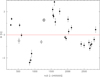 |
Fig. 7 Evolution of the longitudinal component Bℓ during the 8seasons. Open and full symbols represent ESPaDOnS and Narval, respectively. |
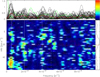 |
Fig. 8 2D Fourier analysis of the Stokes V parameter. The horizontal red line represents the star velocity, 21 km s−1. The vertical white bars represent the three frequencies around 1850 d, 500 d and 250 d, while the dotted white line marks a signal around 200 d. The above picture shows, for each velocity-bin, the Fourier periodograms together with its average (red) and window function (green). On the right is shown the mean-V profile together with the star velocity (red), while the dotted line represents the null polarization level. |
6 The spot model
A star with a localized monopolar magnetic spot on its surface is expected to show the classical S-shaped Zeeman signature (Mathys 1993). In particular, the right and left circular polarization components should be anti-symmetric with respect to the I line profile. As presented in Fig. 6, the five first seasons of observation of Betelgeuse present one dominant polarity and a shape compatible with that expected from the presence of a magnetic spot. However, there are two facts that weaken this simple view, as illustrated for example, by observations N20100300 or N20130908 (Fig. 4). First, the Stokes V profiles are not centered on the rest frame velocity, but are often redshifted by about 10 km s−1 (e.g., Fig. 8), indicating that the magnetic field is located in particular regions of the star that favour downward flows. Second, the left and right circularly polarized fluxes appear to be unequal in absolute value. These observed properties could be interpreted as implying the presence of additional magnetic locations, characterized by different Zeeman intensities and different velocities. Indeed, a configuration with two regions of opposite polarity is commonly seen in Ap stars, even with weak longitudinal magnetic fields and low projected rotation velocity (Aurière et al. 2007), and leads to crossover structures, such as that observed in observation E20121000 (Fig. 4). However, both the redshifted and asymmetric shape of the Stokes V profiles also applies for most of the observed “crossover” configurations (e.g., E20101121 or N20160120), which are unsatisfactorily modeled with one or two equal “spots”. Moreover, the behavior of the Stokes V profiles is not easily interpreted in Seasons 6–8 (Fig. 6), showing very complex structures, definitely far from classical S or crossover shapes. A natural interpretation would be to consider a mix of different magnetic field concentrations having different polarities and velocities. The fact that the signal is weakened by roughly a factor of two for the two later seasons could be due to a dilution of the “spot(s)” of the first seasons. We emphasize that during this same period, the linear polarization signal in both Stokes Q and U is also weakened by a similar factor, although the profiles shapes remain roughly unchanged (Aurière et al. 2016). This strengthens the link between circular and linear polarizations pointed out in the previous section. Aurière et al. (2016) interpreted the linear polarization variations as due to two main bright spots on Betelgeuse. In the following, we continue to apply this spot model to the newly-obtained linear polarization observations described in Table 1, and tentatively extend it to the circular polarization observations.
6.1 Linear polarization
From the shape of both Q and U signals, Aurière et al. (2016) were able to reconstruct the location of the scattering centers at the origin of the linear polarization, leading to two bright spots both near the eastern and southern limbs of the stellar disk (with a 180° uncertainty). This model was fully compatible with quasi-simultaneous high angular resolution observations with VLTI/PIONIER that detected the emergence and variation of a large hot spot at the eastern limb of Betelgeuse (Montargès 2014; Montargès et al. 2016; O’Gorman et al. 2017).
Using our new linear polarimetric data, we used the same model (Aurière et al. 2016) to follow two spots until April 2017. The angular parameters derived from the model are provided in Table 1, and resulting maps are presented in Fig. 10. Even though the signal has decreased in intensity by a factor of about 2.5, the areas of the scattering centers are still more or less located near the eastern and southern limbs on the stellar disk, reflecting a long-term stability of the bright spots, compatible with the results of Sect. 5.
6.2 Circular polarization
Despite the complex magnetic structure expected of a star such as Betelgeuse, rough comparisons performed with solar magnetograms, in addition to magnetohydrodynamics simulations both for main sequence stars (Beeck et al. 2015) or directly related to Betelgeuse (Dorch 2004), show that while complex, the magnetic structures may appear concentrated. Whereas linear polarization is related to scattering anisotropy, interpreted as bright spots, circular polarization can be modeled using several magnetic spots on thestellar surface, mimicking such magnetic concentrations. Each magnetic spot is here characterized using three parameters. First, the width (FWHM) of the left-or-right polarization signal, that should be of the order of that of the Stokes I profile that is, about 20 km s−1. Second, the amplitude (A) of the magnetic field should be adjusted through the extrema of the Stokes V profile. These two parameters lead to the classical S shape, that could be Doppler shifted, the associated velocity (HRV) representing the radial motion of the considered spot and being thus the third parameter. Therefore, each spot is modeled using the (FWHM, A, HRV) parameters. Of course, the complexity of the V signal requires more than one spot most of the time. This is illustrated in Fig. 11, where the resulting fits are presented for two nights (E20101121 and N20140408). For night E20101121, the V profile looks like a classic crossover and as expected two spots of opposite polarity (blue and red profiles) provide an acceptable fit (green profile) superimposed on the observed one. It should be emphasized that each fit has been constrained to the minimum possible number of magnetic spots, through Bayesian marginalization, thus minimizing the risk of overfitting and/or to derive a nonunique solution. The fit associated to night N20140408 requires the presence of four spots, three of positive polarities (red) and one of negative polarity (blue). The fitting procedure was applied to the 30 selected nights presented in Fig. 4, and the results are illustrated in Fig. 12. Compared to the linear polarization Stokes parameters, the Stokes V signatures appear more complex, requiring from one (e.g., N20111208) to five (e.g., N20160120) magnetic spots. However, due to both the weak signal and the simplicity of the model, many configurations are doubtful or even obviously wrong, such as the case of for example, N20140408 or N20161203. Indeed, considering for instance N20140408, the positive polarity does not correspond to any signal.
We then retained the nights where one or two significant spots (i.e., having amplitudes significantlylarger than was typical on a given night), with realistic widths compared to that of the I profile, and we studied the three fitting parameters (FWHM, A, HRV) associated with each spot. On this basis, nights E20140408, E20140900, E20141000, and all nights of 2016 were excluded. The variations derived from the fitting parameters are illustrated in Fig. 13. The first result is that the amplitude A (the dominant polarity) clearly varies on the LSP timescale (about 2000 d). The velocities associated with the magnetic spots have variations closely linked to the amplitude variations, and appear redshifted most of the time (the average spot velocity is about 30 km s−1 i.e., 10 km s−1 above the radial velocity of Betelgeuse), as already noted by Petit et al. (2013). We note that this velocity corresponds to the center of the S shape, and therefore each lobe extends to ± 20 km s−1 and explains the signal already pointed out around 50 km s−1 (see Sects. 3.1 and 5). Thus, conversely to the expansion velocity used by Aurière et al. (2016), we have to deal with structures that appear to be associated with downflows with a mean velocity of about 10 km s−1. Finally, the width parameter appears quite dispersed, spread between 10 and 35 km s−1, whereas the Stokes I profile remains within a 2 km s−1 interval around the mean value of about 20 km s−1, as already noted during the comparison of the signal location between Figs. 8 and 9. In contrast with the width of the I profile, which is integrated over the whole visible disk and is thus relatively stable, the spectral line parameters associated with the left and right polarization for a given magnetic spot appear more localized and hence more sensitive to the local temperature, turbulence or velocity field.
7 Discussion and conclusions
Our observations and modeling establish the presence of a magnetic signal that varies with timescales similar to those of the linear polarization measurements, typically around 2000 d and 300 d. All these polarization signals have been interpreted here in terms of spots, either magnetic spots for the circular polarization or bright spots for the linear polarization.
The complex pattern of the Stokes V signal might be explained by several magnetic spots, each presenting a classic Zeeman profile (S shape) and shifted relative to one another by a given velocity. In Ap stars, the velocity field associated with the Stokes V variations, and in particular the crossover, is entirely dominated by the rotation of the star. For Betelgeuse, the crossover morphology evolves on a timescale of a few months, much less than the expected rotation period of the star, around 17 a (Uitenbroek et al. 1998) or even 31 a (Kervella et al. 2018), so that we can exclude such a scenario. The velocity field should thus concern (sub-)photospheric motions, such as pulsation and/or convection. For cool evolved stars, the favoured pulsation modes are radial, meaning that the whole surface of the star expands or contracts on a timescale of typically a few hundred days, at velocities of a few km s−1 (e.g., Wood et al. 2004).We note that nonradial modes are not excluded, but they should be associated with very low-amplitude motions and would presumably be undetectable. Despite our rough frequency analysis, it appears that the main timescale detected in the polarization parameters is much longer than the radial fundamental period (about 400 d), and hence is rather linked to the Long Secondary Period (LSP). This LSP timescale, about 2000 d for RSGs, may be associated with giant convection cells, that might extend to typically the stellar radius, and have lifetimes of the order of years (Chiavassa et al. 2009, 2010, 2011b).
Giant convection cells as an explanation for the LSP have been studied by Stothers (2010), who provided the typical turnover timescale and velocity of about 2500 d and 7 km s−1 for Betelgeuse, respectively. Aurière et al. (2016) explained the linear polarization through scattering anisotropies due to bright spots. In order to locate these spots on the surface, they introduced an arbitrary expansion velocity, that might be due either to the ascending flow within the bright spot or within the atmosphere, propelled by the locally enhanced luminosity. The circular polarization, being most of the time redshifted, cannot be associated with such an upflow at the center of the bright spot, but it may be associated to the downflow at the edge of the same giant convection cell. The “concentration” of magnetic field at the border of the cell may be the result of the advection flows that act on the magnetic regions and thus on their locations. Such a phenomenon has been studied in the case of the solar supergranulation (Roudier et al. 2016) in order to explain observations showing that a significant part of the flux that appears inside supergranular cells is observed to move toward the photospheric network at their boundary (Gosić et al. 2014). Apart from the Sun, magnetohydrodynamic simulations of the upper layers of convective envelopes of cool main sequence stars have shown that the strong concentration of the magnetic flux in some of the convection downflows leads to a local increase of the field strengths by a factor of 100 (Beeck et al. 2015). In particular, these authors show that the velocity field is responsible for the very inhomogeneous structure of the magnetic field: horizontal outflows from the granules keep the magnetic flux in the downflow regions, while the upflows become nearly field-free. In addition, detailed numerical simulations show that, for Betelgeuse, the field becomes concentrated into elongated structures much thinner than the scale of the giant convection cells (Dorch & Freytag 2003). Thus solar observations and simulations of cool stars provide support for the hypothesis that the magnetic field is located at the edge (i.e., in the sinking part) of the giant convection cells. Our simple model reduces this distribution of magnetic concentrations to just two or three “spots” that suffice to reproduce the observations but that should be interpreted as a representation of a more complex distribution. The spot velocity is sometimes blueshifted; this could be due to a perturbation of the downflow velocity, the motion of a neighboring cell, or the particular projection of the radial velocity, for instance superposed to the rotation velocity, which can amount to 15 km s−1 following Uitenbroek et al. (1998). We note that the velocity field of RSGs might be very complex, as already observed for Betelgeuse in the near IR (Ohnaka et al. 2011), and also as in the case of Antares that presents strong upward and downward velocities across its photosphere and/or its (extended) atmosphere (Ohnaka et al. 2017). In addition to the direct link with giant convection cells, both the circular and linear polarizations have secondary, shorter timescales (down to about three months), that may be related to the advection process of the magnetic field, or to the presence of several bright spots that compete amongst one another for the scattering areas. Moreover, this behavior could also be modulated by radial pulsation modes, although no clear common timescales really emerges apart from the longest one. Finally, rotation modulation, even if the latter is long, may also induce projection effects on the measured polarization.
Thus continuing long-term spectropolarimetric observations suggest a coherent picture in which bright spots trace the upflows of convection cells that are at the origin of the linear polarization, while the downflows of the same convection cells concentrate the observed magnetic field. Such a dynamical picture should be closely linked to the multiple components (e.g., Josselin & Plez 2007) of the surface velocity field. Since pure convective motions seem insufficient to lead to the velocities observed for Antares (Ohnaka et al. 2017), a magnetic component could help to solve this problem. Conversely, it is well known that a nonuniform distribution of the velocity field over the stellar surface may lead to strongly distorted profiles, that coud affect somewhat the classical S shape we used here. Indeed, Mathys (1988) showed that the first moments of both Stokes I and V profiles may be used for the purpose of setting constraints on the magnetic field geometry. As a first step, the characterization of the atmosphericdynamics will be described in a forthcoming paper.
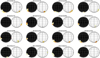 |
Fig. 10 Sequence of images of Betelgeuse from linear polarization for the dates given in Table 1. North is up and east is left for all images. For each date the image (relative intensities) on the left represents the blueshifted signals (spot1) which are located on the visible hemisphere; the image on the right represents the redshifted signals (spot2) which are supposed to correspond to the opposite hemisphere. The crosses show the positions corresponding to the maxima of the linear polarization. The model used is described in Aurière et al. (2016). |
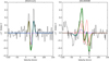 |
Fig. 11 Fit of the V profiles for the nights E20101121 and N20140408. Both positive (red) and negative (blue) magnetic components of each considered magnetic spot, while the total fit is represented with the green line. Whereas the best model for E20101121 requires twomagnetic spots of opposite polarities, N20140408 is represented through four magnetic spots. |
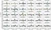 |
Fig. 12 Fit of the V profiles for the observation dates represented in Fig. 4. Both positive (red) and negative (blue) magnetic components are represented for each contributing spots in a given night, while the sum of these contributions is the green line. |
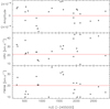 |
Fig. 13 Amplitude, Doppler velocity, and FWHM of each magnetic spot considered (one or two spots per retained night, see text). The stellar rest frame velocity and the mean Stokes I FWHM are indicated by an horizontal red line. |
Acknowledgements
We acknowledge the use of the VALD (Vienna, Austria) and Simbad (CDS, Strasbourg, France) databases. We thank the TBL team for providing service observing with NARVAL. We acknowledge financial support from “Programme National de Physique Stellaire” (PNPS) of CNRS/INSU, France. This project has received funding from the European Union’s Horizon 2020 research and innovation program under the Marie Skodowska-Curie Grant agreement No. 665501 with the research Foundation Flanders (FWO) ([PEGASUS]2 Marie Curie fellowship 12U2717N awarded to MM). GAW acknowledges support in the form of a Discovery Grant from the Natural Sciences and Engineering Research Council (NSERC) of Canada. Finally, the authors are grateful to the anonymous referee for useful remarks and comments.
Appendix
References
- Aurière, M. 2003, in EAS Pub. Ser., eds. Arnaud, J., & Meunier, N., 9, 105 [CrossRef] [Google Scholar]
- Aurière, M., Wade, G. A., Silvester, J., et al. 2007, A&A, 475, 1053 [NASA ADS] [CrossRef] [EDP Sciences] [Google Scholar]
- Aurière, M., Wade, G. A., Konstantinova-Antova, R., et al. 2009, A&A, 504, 231 [NASA ADS] [CrossRef] [EDP Sciences] [Google Scholar]
- Aurière, M., Donati, J.-F., Konstantinova-Antova, R., et al. 2010, A&A, 516, L2 [NASA ADS] [CrossRef] [EDP Sciences] [Google Scholar]
- Aurière, M., Konstantinova-Antova, R., Charbonnel, C., et al. 2015, A&A, 574, A90 [NASA ADS] [CrossRef] [EDP Sciences] [Google Scholar]
- Aurière, M., López Ariste, A., Mathias, P., et al. 2016, A&A, 591, A119 [NASA ADS] [CrossRef] [EDP Sciences] [Google Scholar]
- Babcock, H. W. 1951, ApJ, 114, 1 [NASA ADS] [CrossRef] [Google Scholar]
- Bagnulo, S., Landolfi, M., Landstreet, J. D., et al. 2009, PASP, 121, 993 [NASA ADS] [CrossRef] [Google Scholar]
- Barrick, G., Benedict, T., & Sabin, D. 2010, SPIE, 7735E, 4CB [Google Scholar]
- Bedecarrax, I., Petit, P., Aurière, M., et al. 2013, EAS, 60, 161 [CrossRef] [EDP Sciences] [Google Scholar]
- Beeck, B., Schüssler, M., Cameron, R. H., & Reiners, A. 2015, A&A, 581, A42 [NASA ADS] [CrossRef] [EDP Sciences] [Google Scholar]
- Blazère, A., Petit, P., Lignières, F., et al. 2016, A&A, 586, A97 [NASA ADS] [CrossRef] [EDP Sciences] [Google Scholar]
- Chiavassa, A., Plez, B., Josselin, E., & Freytag, B. 2009, A&A, 506, 1351 [NASA ADS] [CrossRef] [EDP Sciences] [MathSciNet] [Google Scholar]
- Chiavassa, A., Haubois, X., Young, J. S., et al. 2010, A&A, 515, A12 [NASA ADS] [CrossRef] [EDP Sciences] [Google Scholar]
- Chiavassa, A., Freytag, B., Masseron, T., & Plez, B. 2011a, A&A, 535, A22 [NASA ADS] [CrossRef] [EDP Sciences] [Google Scholar]
- Chiavassa, A., Pasquato, E., Jorissen, A., et al. 2011b, A&A, 528, A120 [NASA ADS] [CrossRef] [EDP Sciences] [Google Scholar]
- Donati, J.-F., Semel, M., Carter, B. D., et al. 1997, MNRAS, 291, 658 [NASA ADS] [CrossRef] [MathSciNet] [Google Scholar]
- Donati, J.-F., Catala, C., Landstreet, J., & Petit, P. 2006, ASP Conf. Ser., 358, 362 [Google Scholar]
- Dorch, S. B. F. 2004, A&A, 423, 1101 [NASA ADS] [CrossRef] [EDP Sciences] [Google Scholar]
- Dorch, S. B. F., & Freytag, B. 2003, IAU Symp., 210, 12 [Google Scholar]
- Folsom, C. P., Petit, P., Bouvier, J., et al. 2016, MNRAS, 457, 580 [NASA ADS] [CrossRef] [Google Scholar]
- Freytag, B., Steffen, M., & Dorch, B. 2002, Astron. Nachr., 34, 213 [NASA ADS] [CrossRef] [Google Scholar]
- Gosić, M., Bellot Rubio, L. R., Orozco Suárez, D., Katsukawa, Y., & del Toro Iniesta J. C. 2014, ApJ, 797, 49 [NASA ADS] [CrossRef] [Google Scholar]
- Grunhut, J. H., Wade, G. A., Hanes, D. A., & Alecian, E. 2010, MNRAS, 408, 2290 [NASA ADS] [CrossRef] [Google Scholar]
- Haubois, X., Perrin, G., Lacour, S., et al. 2009, A&A, 508, 923 [NASA ADS] [CrossRef] [EDP Sciences] [Google Scholar]
- Josselin, E., & Plez, B. 2007, A&A, 469, 671 [NASA ADS] [CrossRef] [EDP Sciences] [Google Scholar]
- Kervella, P., Decin, L., Richards, A. S. M., et al. 2018, A&A, 609, A67 [NASA ADS] [CrossRef] [EDP Sciences] [Google Scholar]
- Kiss, L. L., Szabó Gy, M., & Bedding, T. R. 2006, MNRAS, 372, 1721 [Google Scholar]
- Konstantinova-Antova, R., Aurière, M., Charbonnel, C., et al. 2010, A&A, 524, A57 [NASA ADS] [CrossRef] [EDP Sciences] [Google Scholar]
- Kupka, F. G., Piskunof, N. E., Ryabchikova, T. A., et al. 1999, A&AS, 138, 119 [NASA ADS] [CrossRef] [EDP Sciences] [MathSciNet] [PubMed] [Google Scholar]
- Lambert, D. L., Brown, J. A., Hinkle, K. H., & Johnson, H. R. 1984, ApJ, 284, 223 [NASA ADS] [CrossRef] [Google Scholar]
- Lèbre, A., Aurière, M., Fabas, N., et al. 2014, A&A, 561, A85 [NASA ADS] [CrossRef] [EDP Sciences] [Google Scholar]
- Lignières, F., Petit, P., Böhm, T., & Aurière, M. 2009, A&A, 500, L41 [NASA ADS] [CrossRef] [EDP Sciences] [Google Scholar]
- Mathys, G. 1988, A&A, 189, 179 [NASA ADS] [Google Scholar]
- Mathys, G. 1989, Fundamentals of Cosmic Physics, 13, 143 [NASA ADS] [Google Scholar]
- Mathys, G. 1993, ASP Conf. Ser., 44, 232 [NASA ADS] [Google Scholar]
- Montargès, M. 2014, PhD Thesis, Université Pierre et Marie Curie, France [Google Scholar]
- Montargès, M., Kervella, P., Perrin, G., et al. 2016, A&A, 588, A130 [NASA ADS] [CrossRef] [EDP Sciences] [Google Scholar]
- O’Gorman, E., Kervella, P., Harper, G. M., et al. 2017, A&A, 602, L10 [NASA ADS] [CrossRef] [EDP Sciences] [Google Scholar]
- Ohnaka, K., Weigelt, G., Millour, F., et al. 2011, A&A, 529, A163 [NASA ADS] [CrossRef] [EDP Sciences] [Google Scholar]
- Ohnaka, K., Weigelt, G., & Hofmann, K.-H. 2017, Nature, 548, 310 [NASA ADS] [CrossRef] [Google Scholar]
- Percy, J. R., & Khatu, V. C. 2014, J. Am. Assoc. Variable Star Observers, 42, 1 [NASA ADS] [Google Scholar]
- Petit, P., Lignières, F., Aurière, M., et al. 2011, A&A, 532, L13 [NASA ADS] [CrossRef] [EDP Sciences] [Google Scholar]
- Petit, P., Aurière, M., Konstantinova-Antova, R., et al. 2013, Lect. Notes Phys., 857, 231 [NASA ADS] [CrossRef] [Google Scholar]
- Rees, D. E., & Semel, M. 1979, A&A, 74, 1 [Google Scholar]
- Roberts, D. H., Léhar, J., & Dreher, J. W. 1987, AJ, 93, 968 [NASA ADS] [CrossRef] [Google Scholar]
- Roudier, Th., Malherbe, J. M., Rieutord, M., & Frank, Z. 2016, A&A, 590, 121 [Google Scholar]
- Sabin, L., Wade, G. A., Lèbre, A. 2015, MNRAS, 446, 1988 [NASA ADS] [CrossRef] [Google Scholar]
- Schwarzschild, M. 1975, ApJ, 195, 137 [NASA ADS] [CrossRef] [Google Scholar]
- Semel, M., Donati, J.-F., & Rees, D. E. 1993, A&A, 278, 231 [NASA ADS] [Google Scholar]
- Silvester, J., Wade, G. A., & Kochukhov, O. 2012, MNRAS, 426, 1003 [NASA ADS] [CrossRef] [Google Scholar]
- Stellingwerf, R. F. 1978, ApJ, 224, 953 [NASA ADS] [CrossRef] [Google Scholar]
- Stothers, R. 1972, A&A, 18, 325 [NASA ADS] [Google Scholar]
- Stothers, R. 2010, ApJ, 725, 1170 [Google Scholar]
- Stothers, R., & Leung, K. C. 1971, A&A, 10, 290 [NASA ADS] [Google Scholar]
- Tessore, B., Lèbre, A., & Morin, J. 2017, A&A, 603, A129 [NASA ADS] [CrossRef] [EDP Sciences] [Google Scholar]
- Uitenbroek, H., Dupree, A. K., & Gilliland, R. L. 1998, AJ, 116, 2501 [NASA ADS] [CrossRef] [Google Scholar]
- Wade, G. A., Donati, J.-F., Landstreet, J. D., & Shorlin, S. L. S. 2000, MNRAS, 313, 851 [NASA ADS] [CrossRef] [Google Scholar]
- Wood, P. R., Olivier, E. A., & Kawaler, S. D. 2004, ApJ, 604, 800 [NASA ADS] [CrossRef] [Google Scholar]
All Tables
All Figures
|
Fig. 1 Stokes I, Stokes V , and null polarization N1 (blue) and N2 (green) LSD profiles of Betelgeuse for February 14 (ESPaDOnS) and 10 (Narval), 2012. Small vertical lines represent typical error bars. The vertical line corresponds to the heliocentric radial velocity (HRV) of Betelgeuse (about 21 km s−1). |
| In the text | |
|
Fig. 2 IQUV LSD profiles of Betelgeuse for 27 November 2013 and April 8, 2014. Top panel: Stokes I. Middle panel: Stokes Q (blue), U (red), and V (green) signals, where the V signal has been magnified by a factor ten. Bottom panel: null polarization signal N1 , with the same color code as for the Stokes parameters. Small vertical lines represent typical error bars with the same color code. The vertical line corresponds to the HRV of Betelgeuse (about 21 km s−1). |
| In the text | |
|
Fig. 3 StokesQ (blue), U (red), and from the V measurements N1 (continuous)and N2 (dashed) LSD profiles of Betelgeuse for April 08, 2014 (left) and December 18, 2014 (right) obtained with Narval. Small vertical lines represent typical error bars with the same color code. We note that the N1,2 signals have been multiplied by a factor −20. |
| In the text | |
|
Fig. 4 StokesV (red), null polarization N1 (blue) and N2 (green), and I (black) LSD profiles of Betelgeuse for the 30 dates selected as described in Sect. 3.2and spanning along the eight seasons between March 2010 and April 2017 (Table A.1). We note that the UT observation date is encoded for each retained night (see Table A.1). The vertical line corresponds to the HRV of Betelgeuse (about 21 km s−1). |
| In the text | |
|
Fig. 5 Comparison of Stokes V profiles obtained by selecting photospheric lines of low (blue line) and high (red line) magnetic sensitivity according to the Landé factor. Top panel: Betelgeuse on December 9, 2010. Bottom panel: the magnetic M giant EK Boo on March 18, 2009. |
| In the text | |
|
Fig. 6 Variations of polarity during the eight observation seasons 2010–2017 (S1–S8). Open and full symbols represent ESPaDOnS and Narval, respectively. |
| In the text | |
|
Fig. 7 Evolution of the longitudinal component Bℓ during the 8seasons. Open and full symbols represent ESPaDOnS and Narval, respectively. |
| In the text | |
|
Fig. 8 2D Fourier analysis of the Stokes V parameter. The horizontal red line represents the star velocity, 21 km s−1. The vertical white bars represent the three frequencies around 1850 d, 500 d and 250 d, while the dotted white line marks a signal around 200 d. The above picture shows, for each velocity-bin, the Fourier periodograms together with its average (red) and window function (green). On the right is shown the mean-V profile together with the star velocity (red), while the dotted line represents the null polarization level. |
| In the text | |
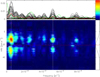 |
Fig. 9 2D Fourier analysis of the Stokes I profiles. Legends are as for Fig. 8. |
| In the text | |
|
Fig. 10 Sequence of images of Betelgeuse from linear polarization for the dates given in Table 1. North is up and east is left for all images. For each date the image (relative intensities) on the left represents the blueshifted signals (spot1) which are located on the visible hemisphere; the image on the right represents the redshifted signals (spot2) which are supposed to correspond to the opposite hemisphere. The crosses show the positions corresponding to the maxima of the linear polarization. The model used is described in Aurière et al. (2016). |
| In the text | |
|
Fig. 11 Fit of the V profiles for the nights E20101121 and N20140408. Both positive (red) and negative (blue) magnetic components of each considered magnetic spot, while the total fit is represented with the green line. Whereas the best model for E20101121 requires twomagnetic spots of opposite polarities, N20140408 is represented through four magnetic spots. |
| In the text | |
|
Fig. 12 Fit of the V profiles for the observation dates represented in Fig. 4. Both positive (red) and negative (blue) magnetic components are represented for each contributing spots in a given night, while the sum of these contributions is the green line. |
| In the text | |
|
Fig. 13 Amplitude, Doppler velocity, and FWHM of each magnetic spot considered (one or two spots per retained night, see text). The stellar rest frame velocity and the mean Stokes I FWHM are indicated by an horizontal red line. |
| In the text | |
Current usage metrics show cumulative count of Article Views (full-text article views including HTML views, PDF and ePub downloads, according to the available data) and Abstracts Views on Vision4Press platform.
Data correspond to usage on the plateform after 2015. The current usage metrics is available 48-96 hours after online publication and is updated daily on week days.
Initial download of the metrics may take a while.