| Issue |
A&A
Volume 614, June 2018
|
|
|---|---|---|
| Article Number | A119 | |
| Number of page(s) | 13 | |
| Section | Interstellar and circumstellar matter | |
| DOI | https://doi.org/10.1051/0004-6361/201732031 | |
| Published online | 28 June 2018 | |
Interaction between a pulsating jet and a surrounding disk wind
A hydrodynamical perspective
1
LERMA, Observatoire de Paris, PSL Research University, CNRS Sorbonne Universités UPMC Univ. Paris 06, 75014 Paris, France
e-mail: This email address is being protected from spambots. You need JavaScript enabled to view it.
2
Instituto de Ciencias Nucleares, Universidad Nacional Autónoma de México, Ap. 70-543, 04510 Cd. Mx., Mexico
3
Univ. Grenoble Alpes, CNRS, IPAG, 38000 Grenoble, France
4
Institut d’Astrophysique Spatiale, CNRS UMR 8617, Université Paris-Sud, 91405 Orsay, France
Received:
3
October
2017
Accepted:
3
January
2017
Abstract
Context. The molecular richness of fast protostellar jets within 20–100 au of their source, despite strong ultraviolet irradiation, remains a challenge for the models investigated so far. Aim.We aim to investigate the effect of interaction between a time-variable jet and a surrounding steady disk wind, to assess the possibility of jet chemical enrichement by the wind, and the characteristic signatures of such a configuration.
Methods. We have constructed an analytic model of a jet bow shock driven into a surrounding slower disk wind in the thin shell approximation. The refilling of the post bow shock cavity from below by the disk wind is also studied. An extension of the model to the case of two or more successive internal working surfaces (IWS) is made. We then compared this analytic model with numerical simulations with and without a surrounding disk wind.
Results. We find that at early times (of order the variability period), jet bow shocks travel in refilled pristine disk wind material, before interacting with the cocoon of older bow shocks. This opens the possibility of bow shock chemical enrichment (if the disk wind is molecular and dusty) and of probing the unperturbed disk wind structure near the jet base. Several distinctive signatures of the presence of a surrounding disk wind are identified, in the bow shock morphology and kinematics. Numerical simulations validate our analytical approach and further show that at large scale, the passage of many jet IWS inside a disk wind produces a stationary V-shaped cavity, closing down onto the axis at a finite distance from the source.
Key words: ISM: jets and outflows / Herbig-Haro objects / shock waves / hydrodynamics / ISM: kinematics and dynamics
© ESO 2018
1. Introduction
Protostellar jets appear intimately linked to the process of mass accretion onto the growing star; their strikingly similar properties across protostellar age, mass, and accretion rate all point to universal ejection and collimation mechanisms (Cabrit 2002; Cabrit et al. 2007; Ellerbroek et al. 2013). Yet, jets from the youngest protostars – so-called Class 0 – are much brighter in molecules (e.g., Tafalla et al. 2000) than jets from more evolved protostars and pre-main sequence stars which are mainly atomic; Molecules have been traced as close as 20–100 au from the source (e.g., Lee et al. 2017; Hodapp & Chini 2014). The origin of this selective molecular richness remains an important issue for models of the jet origin. Three broad scenarios have been considered, with no fully validated answer so far.
In models of ejection from the stellar magnetosphere or the inner disk edge (e.g., Shu et al. 1994; Romanova et al. 2002; Matt & Pudritz 2005; Zanni & Ferreira 2013), the jet would be expected to be dust-free (the grain sublimation radius around a typical solar-mass protostar is Rsub ~ 0.3 au, see for example Yvart et al. 2016). The lack of dust screening then makes the wind extremely sensitive to photodissociation by the accre-tion shock. Chemical models of dust-free winds by Glassgold et al. (1991) found that CO, SiO, and H2O could no longer form at the wind base in the presence of a typical expected level of FUV excess1. Raga et al. (2005) showed that H2 could form further out behind internal shocks. However, the key ions involved are also easily destroyed by FUV photons. Hence, molecule formation in a dust-free jet within 20–100 au of protostars remains an open issue.
A second proposed explanation is that the molecular component of jets may be tracing dusty MHD disk winds launched beyond Rsub, where dust can shield molecules against the FUV field and allow faster H2 reformation. Detailed models are successful at reproducing the higher molecule richness of Class 0 jets (Panoglou et al. 2012) the broad water line components revealed by Herschel/HIFI (Yvart et al. 2016), and the rotation signatures recently resolved by ALMA in the HH212 jet (Lee et al. 2017)and in the slow wider angle wind surrounding it (Tabone et al. 2017). However, the same disk wind models predict that the fastest, SiO-rich streamlines in HH212 (flowing at ~ 100 km s−1) would be launched from 0.05 – 0.2 au, within the dust sublimation radius (Tabone et al. 2017). Hence, this scenario still partly faces the unsolved question of molecule survival in a dust-free wind.
A third scenario is that molecules could be somehow “entrained” from the surroundings into the jet, assumed initially atomic. In a time-dependent jet, travelling internal shocks will squeeze out high-pressure jet material, which then sweeps up the surrounding gas into a curved bowshock. If the surrounding material is molecular, a partly molecular bowshock will result, with a more tenuous “wake” of shocked molecular gas trailing behind it (Raga & Cabrit 1993; Raga et al. 2005). As the next “internal working surface” (IWS) propagates into this wake, it may again produce a molecular jet bowshock. However, after the passage of many such IWS, the wake will be so shock-processed and tenuous that not enough molecules may be left to produce molecular bowshocks close to the jet axis.
In the present paper, we revisit this last scenario in a new light by investigating whether a slower molecular “disk wind” surrounding the jet could help refill the wake and re-inject fresh (unprocessed) molecules into the jet path. This new outlook is prompted by the discovery of a potential molecular disk wind wrapped around the dense axial jet in HH212 (Tabone et al. 2017). We explore this possibility by studying analytically and numerically the propagation of bow shocks driven by a time-variable, inner jet into a surrounding slower disk wind. This scenario may be seen as an extension of the recent modeling work of White et al. (2016) who studied the turbulent mixing layer between a jet and disk wind, with the novel addition of internal working surfaces (IWS) in the jet to produce a stronger coupling between the two outflow components.
Besides our main goal of exploring the impact of a DW on the chemical richness of Class 0 jets, our study has two other important motivations. First, we aim to identify specific signatures in the morphology and kinematics of jet bowshocks that could reveal the presence of a surrounding DW. Secondly, we aim to identify in which regions of space the pristine DW mate-rial would remain unperturbed, for comparison to theoretical DW models.
In the present exploratory study, we have limited ourselves to purely hydrodynamical and cylindrical flows, which allow us to develop an analytical model that greatly helps to capture the main effects of the two-flow interaction, and to understand the numerical results. Also, this is expected to be an optimal case for interaction between the two flows, as magnetic tension would tend to oppose mixing.
The paper is organized as follows. In Sect. 2, we build an analytical model (in the thin shell approximation) for the prop-agation of a bow shock driven by an IWS into a surrounding disk wind. The model is extended to the case of two or more successive IWS. In Sect. 3, we compare the analytic model with axisymmetric simulations of a variable jet + surrounding disk wind configuration, and compare the results with a “reference simulation” in which the same variable jet propagates into a stationary environment. Finally, the results are discussed in Sect. 4.
2. Analytical approach
2.1. Basic equations
We considered the “disk wind + jet” configuration shown in Fig. 1 where a cylindrical jet of radius rj and time-variable velocity vj directed along the z-axis is immersed in a plane-parallel “disk wind” with uniform density ρw and time-independent velocity vw parallel to vj.
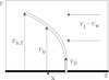 |
Fig. 1 Schematic diagram of the flow around an internal working surface (IWS) in the frame of reference co-moving with the IWS at velocity vz = vj (a similar configuration would apply for the leading working surface of a jet). The thick, horizontal line at the bottom of the graph is the jet (with a gap showing the position of the IWS). The working surface ejects jet material sideways at an initial velocity v0 into the slower disk wind, which in this frame of reference moves towards the outflow source at velocity vj – vw. The distance x is measured towards the outflow source.The shape of the thin shell bow shock is given by rb(x) (see Eq. (5)), and terminates at the cylindrical radius rb; f(t) with t the time elapsed since formation of the IWS (see Eq. (8)). |
The jet velocity variation is such that an internal working surface is produced within the jet beam. In the following derivations, we assume that the working surface is formed at t = 0 at the position of the source (i.e., z = 0), and that it then travels at a constant velocity vj (for t > 0). Such a working surface could be produced, for example, by an outflow velocity with a constant value v1 < vj for t < 0, jumping to a constant value v2 > vj for t ≥ 0. Note that if the shock is produced at distance zs > 0 at a time ts > 0, the equations below remain valid with the transformation z → z – zs and t → t – ts.
In a frame of reference moving with the internal working surface (see Fig. 1) the over-pressured shocked jet material which is ejected sideways from the working surface interacts with the slower moving, surrounding disk wind. In the strong radiative cooling limit, this sideways ejection leads to the formation of a thin-shell bow shock, which sweeps up material of the surrounding disk wind, flowing towards the source at a relative velocity (vj–vw).
Assuming full mixing between jet and disk wind material, we can write the mass, r and x-momentum conservation equations at any point of radius rb along this thin-shell (r, x, and rb being defined in Fig. 1) as: (1)
(1)
 (2)
(2)
 (3)
(3)
where ṁ is the mass rate,  the r-momentum rate and
  the x-momentum rate of the mixed jet + disk wind material flowing along the thin-shell bow shock, and ṁo and v0 are the mass rate and velocity (respectively) at which jet material is initially ejected sideways by the working surface. These equations have straightforward interpretations. As an illustration, we point out that Eq. (2) states that the radial momentum of the material flowing along the thin shell remains constant over time (which is due to the fact that the disk wind material adds no r-momentum), so that its radial velocity vr decreases as ṁ increases, the r-momentum being shared with a larger amount of zero r-momentum material from the disk wind.
The mass rate ṁo and velocity v0 of the sideways ejected material are determined only by the properties of the working surface. For a highly radiative working surface, we would expect the post-shock jet material to cool to ~ 104 K before exiting sonically into the disk wind. Therefore, we would expect v0 ∼ 10 km s−1. The mass rate ṁ0 will have values of the order of the (time-dependent) mass loss rate  in the jet beam.
We note that although our basic equations are similar to those of Ostriker et al. (2001) our approaches and derived equations will differ. They considered only the case of the leading jet bowshock propagating in a medium at rest (vw = 0), so that the injected mass and momentum rates ṁ0 and ṁ0vo were expressed as a function of the velocity of the shock and the jet radius. Here, we keep ṁ0 and v0 as explicit parameters, so that we can consider a moving surrounding disk wind of arbitrary velocity vw, and an arbitrarily small rj.
2.2 Shape of the bow shock shell
For a disk wind with position-independent density ρw and velocity vw, the integrals in Eqs. (1) and (3) can be trivially performed, and from the ratio of Eqs. (2) and (3) one obtains the differential equation of rb(x) : (4)
(4)
which can be integrated to obtain the shape of the thin shell bow shock as a function of x in the IWS reference frame: (5)
(5)
where we defined the characteristic scale2
 (6)
(6)
Clearly, as the thin shell bow shock began to grow at t = 0, the solution given by Eq. (5) must terminate at a finite maximum radius rb,f (see Fig. 1). The growth of this outer radius with time can be calculated combining Eqs. (1) and (2) to obtain: (7)
(7)
which can be integrated with the boundary condition rb,f to obtain rb,f(t) at the current time t:![Mathematical equation: $$ \frac{1}{\gamma {L}_0^2}\left[{r}_{b,f}^3-{r}_j^3+3{r}_j^2({r}_j-{r}_{b,f})\right]+{r}_{b,f}-{r}_j={v}_0t, $$](/articles/aa/full_html/2018/06/aa32031-17/aa32031-17-eq11.gif) (8)
(8)
with (9)
(9)
Now, in order to obtain the shape of the bowshock shell in the source frame (z, r) (see Fig. 2, cyan curve), when the IWS is located at distance zj from the source, we simply insert the relation x = (zj – zb
) into Eq. (5) and t = t ≡ zj/vj in Eq. (8). In the “narrow jet” limit where rj→ 0, the thin shell bow shock has the simple cubic shape given by equation: (10)
(10)
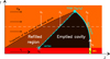 |
Fig. 2 Schematic diagram showing the flow around a working surface of a jet (in this case the leading working surface, but the diagram also applies for an internal working surface). The jet is the horizontal, red rectangle at the bottom of the graph, with the source located at z = 0. The working surface in yellow is located at a distance zj from the source and travels at a velocity vj. It ejects material away from the axis at an initial velocity v0. The jet is surrounded by a “disk wind”, which travels along the outflow axis at a velocity vw. The shape of the thin-shell bow shock (thick cyan line) is given by zb as a function of r and ends at the edge of the bow wing (cyan point; zb f, rb f). The bow shock leaves behind a “cavity” (black region), which is partially refilled by the disk wind (brown region). The boundaries of the initial swept up cavity (in black dashed line) and of the refilled region (cyan dash-dotted line) are given by zf an zc (respectively) as a function of cylindrical radius r (see Eqs. (14) and (15)). |
ending at the maximum “outer edge” radius rb, f (see the cyan dot in Fig. 2) given by Eq. (8) evaluated at t = tj: (11)
(11)
For a “wide jet” where  is no longer negligible, the corresponding equations can also straightforwardly be obtained from Eqs. (5) and (8), and are given in Appendix 5. In the following, we consider the narrow jet regime, which leads to simpler equations.
2.3 The post-bow shock cavity
Let us now consider the trajectory rf(zf) described in the z, r plane by the outer edge of the thin shell bow shock at earlier times, when the IWS travelled from its formation point z = 0 at t = 0 to its current location zj at time tj. This trajectory will define the shape of the volume swept out by the travelling and expanding bowshock into the slower disk wind (see Fig. 2, dashed black line).
At an earlier time tf (0 ≤ tf ≤ tj), the bowshock terminated at an outer radius rf ≤ rb, f given by Eq. (11) with t j= : tf
 (12)
(12)
The distance zf from the source where this radius rf was reached is obtained from Eq. (10) by setting zb = zf, rb = rf and zj = vjtf:
 (13)
(13)
Combining Eqs. (12) and (13) to eliminate tf, and recalling that γ = (vj – vw/)v0 we then obtain the shape rf(zf) of the cavity swept by the (growing) edge of the bow shock wing associated with the travelling internal working surface (see dashed black curve in Fig. 2) : (14)
(14)
2.4 Refilling of the cavity by the disk wind
Of course, as soon as the bow shock wing has passed by, the disk wind (travelling in the z-direction at a velocity vw, see Fig. 2) immediately starts to refill the swept-up cavity. For a given radius rf(zf) along the boundary of the swept-up volume, the refilling by the disk wind will thus start at the time tf (given by Eq. (13)) when the bowshock edge reached this position; at the present time tj the disk wind will have refilled a region of length (tj – tf)vw along the z-axis. The boundary between the wind-refilled region and the emptied cavity thus has a locus zc(rc) (see the cyan dash-dotted line in Fig. 2) given by: (15)
(15)
where for the second equality we have used Eqs. (12) and (13) and set rc = rf.
Therefore, the slower disk wind refills the cavity swept by the bow shock except for an inner, conical “hole” with half-opening angle α = arctan γ−1 = arctan[v0 / (vj–vw)]. The conical cavity is attached to the wings of the bow shock at (zbf, rbf), and its vertex along the jet axis is located at a distance from the source za = vwtj = zj (vw/vj) (see Eq. (15) with rc = 0 and cyan asterisk in Fig. 2).
Figure 3 shows the analytical flow configurations obtained at three different evolutionary times (corresponding to za = vwtj = zj (vw/vj), and), and for two choices of the wind velocity (vw = 0 andvw = 0.4vj). In the two models, we have set  . vo = 0.2 The model with vw = 0 (left frames of Fig. 3) produces a cavity which does not fill up. For vw = 0.4vj (right frames of Fig. 3), the bow shock has a more stubby shape compared to the vw = 0 bow shock (L0 is larger) and the cavity which it leaves behind is partially refilled by the disk wind (brown region).
 |
Fig. 3 Time evolution of the bow shock + cavity flow predicted by the analytic model for two choices of the wind velocity: vw = 0 (leftframe) and vw = 0.4vj (right frame). The dark region is the empty part of the cavity (swept-up in the thin shell bow shock) and the brown region is the part of the cavity that has been refilled by the disk wind (this region being of course absent in the vw = 0 model of the left frame). For both models, we show snapshots corresponding to t = 2L0/Vj, 4L0/Vj, and 8L0/vj), which result in positions zj = 2L0, 4L0, and 8L0 for the working surface (see the labels on the top left of each frame). Both models have v0 = 0.2vj |
2.5 Kinematics along the shell
From Eqs. (1)–(3), it is straightforward to show that for a narrow jet surrounded by a homogeneous disk wind, the radial and axial velocities (in the source rest frame) of the well-mixed thin shell material as a function of cylindrical radius rb are : (16)
(16)
 (17)
(17)
where for the second equation we have also considered that vz = vj – vx (see Figs. 1 and 2). In evaluating the radial velocities, one should keep in mind that the radius rb is always smaller than the rb,f value given by Eq. (11).
As expected, we find the following asymptotic limits:
-
vr has an initial value v0 for rb → 0 (i.e., as it leaves the jet working surface) and goes to 0 at large radii (as the radial momentum of the thin shell bow shock is shared with an increasing mass of disk wind),
-
vz has an initial value vj when it leaves the working surface (rb → 0), and for large radii tends to the disk wind velocity vm.
Equations (16) and (17) give the velocity of the well-mixed material within the thin shell bow shock. These velocities correspond to the Doppler velocities observed in an astronomical observation provided that the emission does indeed come from fully-mixed material.
Another extreme limit is if the emission is actually dominated by the gas that has just gone through the bow shock and which is not yet mixed with the thin shell flow material. In this case, the axial and radial velocities of the emitting material would correspond to the velocity directly behind a highly compressive radiative shock. For such a shock, the velocity of the post shock flow (measured in the reference system moving with the bow shock) is basically equal to the projection of the incoming flow velocity parallel to the shock front. It is straightforward to show that in this case the immediate post shock radial and axial velocities of the emitting material in the source rest frame are given – in the narrow jet limit – by: (18)
(18)
 (19)
(19)
We note that while vz,ps has the same asymptotic limits as vz in the full mixing case (see Eqs. (17) and (19)), the radial postshock velocity vr,ps tends to zero both for rb → 0 and for rb → ∞ (see Eq. (18)), reaching a maximum value of (vj – vw)/2 for a radius equal to  This peak value for the radial velocity is a general result of bow shock kinematics, valid regardless of the shape of the bow shock, which was first derived by Hartigan et al. (1987).
By combining Eqs. (16)– (19) with Eq. (10) it is straightforward to obtain the axial and radial velocities as a function of the distance z along the symmetry axis. Examples of these dependencies are shown in the following section.
2.6 A dimensional example
We now consider a particular model of an internal working surface moving at a velocity vj = 100 km s−1, located at zj = 1016 cm along the z-axis and ejecting side way material at a rate ṁ0 = 10−8 Mʘ yr−1 with a lateral ejection velocity v0 = 10 km s−1.
For the surrounding disk wind, we assume a number density of atomic nuclei nw = ρw/1.4 mH = 104 cm−3 and velocities vw = 0 and vw = 40 km s−1. With these parameters, we obtain L0 = 5.2 × 1014 cm (for vw = 0) and L0 = 8.7 × 1014 cm (for vw = 40 km s−1). Note that Jṁ0 and ρw are only involved in the shape and kinematic equations through L0 ∞ (ṁ0/ρw)1/2, so that only their ratio actually matters in defining the flow properties.
For these two working surfaces, we obtain the shapes, and the radial and axial velocities (as a function of z) shown in Fig. 4. From this figure, it is clear that for the vw = 40 km s−1 model we obtain a flatter working surface than for the vw = 0 case, because L0 is larger.
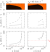 |
Fig. 4 Shape of the bow shock and the cavity (top), radial velocities vr (center) and axial velocities vz (bottom) for the two models discussed in the text. The solid curves show the velocities of the well-mixed material within the thin shell flow, and the dashed curves show the immediate post-bow shock velocities. The dotted red line shows vz = vw. |
The velocities of the fully mixed thin shell material (shown with solid lines in Fig. 4) have the following behaviors:
-
vr has a value of v0 = 10 km s−1 at z = zj, and monotonically decreases toward (but not reaching) zero for decreasing values of z;
-
vz (lower plots of Fig. 4) has a value of vj = 100 km s−1 at zj, and monotonically decreases for lower values of z, towards (but not reaching) an asymptotic limit of vw.
The immediate post-bow shock velocities (shown with dashed lines in Fig. 4) have the following behaviors:
-
vr,ps (central plots of Fig. 4) is zero at the apex of the bow shock surface at z = zj, and rapidly grows to a maximum value of 50 km s−1 (for vw = 0) and 30 km s−1 (for vw = 40 km s−1), this value corresponding to (vj – vw)/2, as discussed in the previous section is reached at
 . The radial velocity then decreases again at smaller z until the end of the bowshock wings;
 -
the axial velocity vzps has the same qualitative behavior as the well-mixed vz (see above), but with a different functional form that approaches faster its limit vw in the bowshock wings.
We expect that in reality, due to incomplete mixing, the emitting material will have axial and radial velocities between the fully-mixed layer and immediate post-bow shock velocities shown in Fig. 4. The difference between these two velocities is particularly important for the radial component of the velocity of the emitting material.
2.7. Successive bow shocks
In the previous section, we assumed that the bow shock associated with an internal working surface travels through undisturbed disk wind material. However, we saw that the cavity formed behind it is only partially refilled by fresh disk wind. Therefore, a second bow shock will travel into a disk wind structure containing an empty, conical cavity left behind by the first bow shock.
We now assume that the variable ejection velocity of the jet produces a second working surface at z = 0 at a time τj, which also travels along the jet axis with the same velocity vj as the first working surface. Figure 5 illustrates three steps of the propagation of this second working surface.
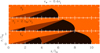 |
Fig. 5 Time evolution of two successive bow shocks and the cavities predicted by the analytical model. The first bow shock is ejected at t = 0, the second shock is formed at time t = τj when the first bow shock is at z = vjτj taken here as 6L0 (top). At a time t = τj + 2L0/vj, the second bow shock is still propagating in the undisturbed disk wind material (center). At a time tc the second bow shock catches up the emptied cavity of the first bow shock at its vertex (bottom). |
At t = τj (Fig. 5, first panel) the first working surface is at a distance zj1 = vjτj from the outflow source and its cavity is partially filled with fresh disk wind material, while the second working surface has not yet expanded. At a time τj < t < tc (Fig. 5, center) the second bow shock travels in unperturbed, pristine disk wind material that refilled the cavity behind the first bowshock; hence its shape and kinematics are still given by the same equations derived above for the leading internal working surface, and any molecules present in the disk wind can enter the second bowshock. At a time t = tc (Fig. 5, bottom panel) the apex of the second bowshock just catches up with the vertex of the conical cavity emptied by the first bow shock and not refilled by the disk wind.
To obtain the time tc, we note that at any time t (τj < t < tc), the position of the apex of the second bow shock is zj2 = vj(t – τj) and the position of the vertex of the empty cavity behind the first bow shock is za1 = vwt. By equating these two quantities we get (20)
(20)
This interaction occurs at a distance lc from the source: (21)
(21)
where Δz = Tjvj denotes the distance between two successive IWS. Unless vw is very close to vj, we find that lc is of the order of a few times the typical IWS spacing.
Our model thus predicts that no more pristine unperturbed disk wind material can remain close to the jet axis beyond z = lc. When the second IWS reaches z > lc, the central region of its bow shock shell propagates into the emptied cavity left behind by the previous IWS. This second bow shock shell will in general become less curved than the first one, because its central region travels into a low density cavity instead of unperturbed disk wind.
3. Numerical simulations
In the previous section, we proposed a simple analytical “thin-shell” model that describes the morphology and the kinematics of a bow shock produced by a pulsating jet travelling in a surrounding disk wind. We especially show that the disk wind refills up part of the cavity carved by the bow shock, allowing us to observe pristine disk wind close the source. For successive bow shocks, bow shocks travels in an undisturbed disk wind up to a critical distance l c. Above this altitude, bow shock shells interact with each other and analytical models can only be heuristic.
In this section, we present numerical simulations that start with the simple configuration adopted above, first to determine to what extent the analytical model can be used to describe a realistic situation – e.g., with a partial mixing – and secondly to study briefly the long term evolution of the interacting bow shock shells.
3.1. Numerical method and setup
We carry out numerical simulations of a variable ejection jet surrounded by a wide “disk wind” outflow. We have implemented the new HD numerical code Coyotl which solves the “2.5D” Euler ideal fluid equations in cylindrical coordinates: (22)
(22)
where U is the vector of conserved quantities (23)
(23)
with fluxes in the r- and z directions given, respectively, by (24)
(24)
 (25)
(25)
ni are passive scalars used to separate the jet from the disk-wind material in the flow. Assuming an ideal equation of state, the total energy density e is (26)
(26)
and the source term is (27)
(27)
where the cooling function Λ(T) is the parametrized atomic/ionic cooling term of Raga & Canto (1989), which approximates the cooling curve of Raymond et al. (1976) for temperatures above 104 K.
The numerical scheme is based on a second order Godunov method with an HLLC Riemann solver (Toro 1999). The calculation of the fluxes and data reconstruction uses the second order scheme described by Falle (1991). This algorithm solves Euler equations in a true cylindrical coordinate system as written in Eq. (22) and calculates the cell gradients through the center of gravity of the cylindrical cells.
We ran two simulations: a reference simulation called no-DW model, with vw = 0 (i.e., a jet in a stationary ambient medium) and a simulation with vw = 0.4vj called DW model. To follow the refilling of the cavity close to the source and the interaction between various shells, we integrate equations on a 2000 au × 350 au domain, with a resolution of 1 au per cell. All jet and wind parameters except vw are kept equal between the two simulations, and are summarized in Table 1.
Model parameters.
Our initial conditions have an inner, constant velocity jet filling the r < rj region at all z, and the disk wind (or external stationary medium) filling the rest of the computational domain. This setup differs from the standard jet initialization in which the jet is introduced only in a small region around z ≃ 0 and then propagates through the domain, producing a transient with a leading jet bow shock that sweeps aside the ambient medium (Blondin et al. 1990; de Gouveia dal Pino & Benz 1993). By initializing our simulations with a jet that already extends across the whole range of z, we do not perturb the surrounding medium with the transient leading jet bow shock and we can directly follow the interaction between an IWS and the unperturbed disk wind close to the outflow source.
In order to form IWS in the jet, we impose a saw-tooth ejection variability with a mean velocity vj, a velocity jump ∂vj and a period Δτj.The ejection velocity is assumed to rise linearly from vj – ∂vj/2 to vj + ∂vj/2 during a time-lapse ƞΔτj and to linearly decrease over a time (1 – η)Δτj back to a velocity vj – δvj/2. Using the small amplitude velocity variability approximation of (Raga et al. 1990), we estimate that for our chosen parameters in Table 1 this variability will produce an internal working surface in the jet at time tS = 5 yr and distance zS = (vj – δvj/2)2ηΔτj/δvj = 75 au from the central source,and that the working surface will travel in the jet at a velocity vj = 96 km s−1.
We adopt a jet radius rj = 20 au consistent with the width of the HH 212 molecular jet obtained from VLBI measurements
by Claussen et al. (1998) and with the widths of atomic jets estimated by Dougados et al. (2000) close to the source. The density contrast between the jet and the wind is chosen to be sufficiently high (ρj /ρw = 29) to produce wide bow shock shell. Temperatures are chosen to insure a transverse pressure equilibrium between the jet and the wind. Note that simulations are not very sensitive to the jet temperature since strong internal shocks cooled down by atomic lines set the temperature of the IWS at T ∼ 104 K.
The boundary conditions are reflecting on the symmetry axis (r = 0) and outflowing in the outer radial and axial cells. On the z = 0 boundary, we introduce the jet by imposing fixed constant physical conditions for r < rj. For r > rj we impose either the disk wind physical conditions, or a reflecting condition (for the reference simulation with vw = 0). In order to avoid numerical problems due to the z-velocity shear between the jet and the surrounding disk wind we put a velocity gradient on three cells (i.e., 3 au) at the outer edge of the jet inflow.
3.2. Single bow shock propagation
Figure 6 shows snapshots of the no-DW simulation (two frames on the left) and of the DW simulation (two frames on the right) after a t = 48 yr time integration, which is larger than the ejection variability period of 33 yr (see Table 1). The first internal working surface (IWS) has travelled to a distance of 995 au from the source, and a second IWS to 355 au. In this subsection, we study successively the shape of the first bow shock shell, the refilling of the cavity behind it, and the kinematics of the shell, comparing each of them with our analytical predictions.
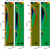 |
Fig. 6 Maps of density and pressure for the reference no-DW simulation with vw = 0 (left) and the DW simulation with vw = 0.4vj(right) at a time t = 48 yr. Color scales on top are in g cm−3 for density and in dyn cm−2 for pressure. White contours show the locus of 50% mixing ratio between jet and disk-wind/ambient material. The cyan curve shows a fit (to the numerical results) by the analytic shell shape in Eq. (11), with L0 = 65 au (left) and 108 au (right). The cyan dot indicates the maximum radius of the shell, the cyan asterix indicates the predicted vertex of the empty conical cavity left behind the shell, and the cyan dash-dotted line is the analytical predicted boundary between the emptied cavity and the region refilled from below by fresh disk wind (see Fig. 2 and Eq. (15)). |
3.2.1. Shape of the bow shock shell
The cyan curves in Fig. 6 show that the bow shock shells in the two simulations can be well fitted with the cubic analytic solution for the thin-shell (Eq. (5)), with values for the characteristic scale L0 = 65 au for the reference no-DW simulation and L0 = 108 au for the DW simulation. In the simulations, the sideways ejection velocity v0 and mass-flux ṁ0 (see Sect. 2) are a result of the IWS shock configuration, which compresses the jet material and ejects it sideways. Since the two simulations only differ in the presence or lack of a surrounding disk wind, the jet IWS in the two simulations have similar characteristics. We then expect that ṁ0v0 is the same, and that L0 should vary with the wind velocity as L0k (vj – vW)−1 (see Eq. (6)). The values of L0 found above by fitting the shell shape are indeed consistent with this expectation.
The cyan dots on the leading bow shock wings in Fig. 6 indicate the maximum radius of the bow shock shell as observed in the numerical simulations, rmax = 133 au in the no-DW and rmax = 137 au in the DW cases. Assuming that it corresponds to the current position of the edge of the thin shell (rbf, zbf), as defined in Fig. 2, our analytic model predicts that rbf depends on L0 and v0 through Eq. (11) or (A.2). With L0 = 65, 108 au, we would deduce v0 = 27, 19 km s−1 for the no-DW and DW simulations, respectively.
To obtain a direct measurement of v0, we plot in Fig. 7 a transverse cut of the radial velocity vr at the position of the leading working surface (z = 993 au) in the DW simulation. Inside the IWS, because of both the adiabatic expansion and the mass flux across the IWS, vr increases from zero to a maximum velocity of 14 km s−1. This direct measurement of v0 is smaller than the values of 27, 19 km s−1 inferred from the maximum radius of the shell in our simulations using Eq. (11) (see above). However, we note that taking v0 = 14 km s−1 (its real value), the predicted rbf would be rbf = 111 au in the no-DW case and rbf = 121 au in the DW case, only slightly smaller than the rmax found in our simulations.
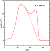 |
Fig. 7 Transverse cut across the flow at the IWS location (z = 993 au) in the no-DW time-frame shown in Fig. 6. This cut shows the radial velocity as a function of distance from the jet axis in solid line. We also plot the radial velocity weighted by the abundance of the jet tracer with a dashed line. The radial velocity first grows outwards, reaches a maximum velocity of ≈ 14 km s−1 at a radius of ∼ 25 au (somewhat larger than the 20 au initial jet radius), and then remains with values > 10 km s−1 until it drops sharply to 0 at r ∼ 50 au. The velocity maximum at r ∼ 25 au corresponds to the shock against the jet material. The second maximum at r ∼ 50 au is the shock that propagates in the disk-wind and the zero radial velocity material at larger radii is the undisturbed disk wind. |
This slight difference in outer radius between the analytic model and the numerical simulations could be a result of several effects:
-
the analytic model assumes a working surface with a time-independent, sideways ejection, while the numerical simulation has an IWS with time–dependent sideways ejection that depends on the evolution of the IWS shocks. The IWS in the simulations produces a higher sideways velocity at early times (v0 ∼ 18 km s−1)3, closer to the values deduced from the analytic cavity shapes;
-
in the numerical simulation, the sideways ejection from the IWS is not highly super-sonic. The thermal gas pressure is therefore expected to be an additional source of sideways momentum for the shell (an effect not included in our momentum conserving analytic model); this will act to produce a higher effective v0;
-
similarly, the thermal pressure in the head of the bow shock driven into the surrounding environment will result in a sideways push which is not present in the momentum conserving analytic model;
-
the numerical simulations do not have instant mixing between the sideways ejected jet material and the shocked environment (or disk wind), as assumed in the analytic model. Since the immediate post shock velocity in the radial direction is generally greater that the radial mean shell velocity (see example in Fig. 4), the growth rate of the bow shock can be enhanced. In the reference frame of the IWS (see Fig. 1), the non-mixed material will “slide” along the shell surface, extending rb,f to larger values.
Lee et al. (2001) found in their simulations similar disagreements between direct measurements of the sideways momentum ejected by the IWS and the momentum estimated from the fitted shape of their analytic shell model.
3.2.2. Cavity refilling
The asterisk in cyan in each panel of Fig. 6 indicates the location of the vertex of the emptied cavity as predicted from the analytic model (see Fig. 2). For the no-DW simulation, this point is located at the shock formation position (zs = 75 au) whereas for the DW simulation this point is located at  . We also plot in cyan dash– dotted the line connecting this vertex to r
max, which traces the boundary predicted by the analytical model between the emptied swept-out conical cavity and the unperturbed surrounding medium/refilled disk wind (see black conical region in Fig. 2). Three important features can be seen.
. We also plot in cyan dash– dotted the line connecting this vertex to r
max, which traces the boundary predicted by the analytical model between the emptied swept-out conical cavity and the unperturbed surrounding medium/refilled disk wind (see black conical region in Fig. 2). Three important features can be seen.
First, in both numerical simulations, the emptied cavity predicted by the analytical thin-shell model, i.e. the conical volume inside the dash-dotted cyan line, is not really empty, but partially filled with a cocoon of low density and pressure material. No unperturbed ambient gas or disk wind can be left inside this volume (in black in Fig. 3), which was entirely swept-out by the growing shell during the IWS propagation. Hence this cocoon is made of shocked material that did not fully mix in the shell, and re-expanded in the low-pressure cavity behind it, refilling it “from above”. The white contour, which denotes the surface of 50% jet/environment mixing fraction (obtained following a passive scalar) shows that the cocoon is mainly filled with jet material close to the axis, where the shell mass is dominated by gas ejected from the IWS. Further from the axis and closer to the theoretical boundary (cyan dash-dot line) it is filled by ambient material that was swept up by the bowshock and re-expanded behind it.
Secondly, the boundary with unperturbed ambient or disk wind material closes back to the axis at the predicted vertex position (see cyan asterisk Fig. 6), but is delimited by a weak shock that extends slightly outside from the predicted analytical boundary (dash-dotted cyan line Fig. 6) . In the no-DW model, the analytical boundary represents the trajectory of the edge of the bow shock (zc = zf in the case vw = 0). Hence, this weak shock is produced by the supersonic motion of the high-pressure edge of the bow shock (rb,f, zb,f) in the static surrounding medium. This launches a weak outward shock that repels the boundary of the unperturbed ambient material slightly outside the predicted cavity boundary (in cyan dash-dotted line). In the presence of a supersonic disk wind, the weak shock front is advected away from the source so that it still closes back on-axis at the predicted vertex position za. Hence, Eq. (15) gives a strong limit on the boundary between perturbed and unperturbed material.
Thirdly, in the presence of a disk-wind, the region between the predicted cavity boundary (cyan dash-dotted line) and the weak shock front outside it is refilled by fresh disk wind material coming from below. To analyse this process we show in Fig. 8 density and velocity maps of the region around the leading bow shock of the DW simulation. The dashed white contours show 10 %, 0.1 %, and 0.001 % jet material mixing fractions. Material that went through the bowshock and re-expanded in the cocoon has also been partially mixed with jet material. As a consequence, regions where no jet material is observed are regions where the disk wind has refilled the cocoon from below. The location of the last, outer contour (corresponding to a 10−5 jet material mixing fraction) shows that the weak outer shock front propagates into un-mixed, fresh DW material. This material manages to cross the weak shock to refill from below the bottom part of the swept-out cavity.
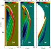 |
Fig. 8 Zoom of the leading IWS of the simulation with a surrounding disk wind at time t = 48 yr. Left: density stratification (with the logarithmic color scale given by the top bar in g cm−3), center: radial velocity (with the linear scale of top bar in km s͔–1) and right: axial velocity structure (with the linear scale of the top bar in km s−1). The white contours show the surfaces of 50 % (solid line), 10 %, 0.1 % and 0.001 % (outer contour) jet material mixing fractions. The cyan asterisk is the predicted vertex of the cavity, the cyan dash-dotted line in the predicted boundary of the cavity, and the cyan curve is the fitted shape of the bow shock. |
The weak shock provides a slight push outwards to the refilling DW, with radial velocities that vary from + 6 km s =1 to + 3 km s−1 along the shock front (middle panel of Fig. 8), similar to the adiabatic sound speed of the disk wind (csw ≈ 2.8 km s−1). The weak shock also reduces the DW inflow velocity vz to values slightly below vw = 0.4vj = 38.4 km s−1 (right panel of Fig. 8). However, refilling remains efficient up to the locus predicted by our analytical model (dash-dotted cyan line), as the jet mixing fraction there remains very small (≃ 0.1 %). The presence of the weak shock does not appear to significantly modify the extent of DW refilling compared to analytical expectations.
In summary, we can therefore distinguish in our simulations three refilling regions behind the bowshock:
-
a low density cocoon trailing the bow shock, that is refilled from above by shell material re-expanding into the emptied cavity. This region is mainly composed of jet material close to the apex of the bow shock, and of shocked swept-up disk wind material behind the wings of the bowshock;
-
an intermediate region (outside the cyan dash-dotted line and inside the weak shock closing the cavity) refilled from below by weakly shocked disk wind material;
-
a region upstream of the weak shock closing the cavity, that is refilled by unperturbed fresh disk wind keeping its initial physical conditions.
3.2.3. Kinematics
We now compare the kinematics in both simulations with our analytical predictions. Figure 9 shows “position-velocity” (PV) diagrams for vr and vz as a function of distance z along the flow axis. In order to enhance the contribution from the material that has just been shocked, each pixel in a snap shot has been weighted by the cube of the pressure p3 times the elementary volume 2πrΔrΔz. Using this weighting, the maximum intensity (in yellow and orange shades) at each position in the PV diagrams then traces the velocity in the shell. The separation between material originating mainly from the jet or mainly from the surroundings/disk wind is done using a passive scalar. The predicted mixed shell velocities (Eqs. (16) and (17)) are shown in blue, and the predicted immediate post-bowshock velocities (Eqs. (18) and (19)) are shown in magenta. Following the discussion of Fig. 7, we take v0 = 14 km s−1.
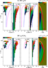 |
Fig. 9 Longitudinal position-velocity (PV) diagrams for the no DW simulation (top) and the DW simulation (bottom). From left to right: vr for the jet material only, vr for the surrounding material only, vz for the jet material only, vz for the surrounding material only, and density stratification. The ordinate of all frames is position along the outflow axis (in au). The color scale in the PVs is scaled by volume × cube of pressure so as to be maximum (in red and yellow shades) for shocked material in the shell, while the color scale for density is in g cm−3. Blue curves are predicted velocities in the full mixing hypothesis (Eqs. (16) and (17)), while magenta curves are the predicted immediate-post shock velocities (Eqs. (18) and (19)). |
In the vr PV diagrams of the surrounding material, the expansion velocities of shocked material in the shell (orange shading) are always larger than predicted by the (blue) full-mixing curve (except very close to the bow shock apex where the shear is maximum). The simulation more closely follows the immediate post-bow shock velocity curve (magenta), indicating that high-pressure shocked material in the shell is not fully mixed in our simulations. Conversely, the vr PV diagram of the jet material decreases monotonically along the bow shock wing with velocities always slightly smaller than the full mixing velocity curve (in blue).
Concerning the velocity along the jet z-axis, the vz values for jet material lie close to, or slightly above the full mixing curve in blue. The vz PV diagrams for the surrounding material generally show smaller vz than predicted by the full mixing curves. The high-pressure swept-up shell material (in orange) lies close to the immediate post-shock velocities (magenta curve).
The relatively small vr velocities and large vz velocities observed in the jet dominated material indicate that even if the full mixing hypothesis does not hold, the momentum is still conserved: if the velocities of the swept-up surrounding material are greater than expected from the full mixing hypothesis, then the velocities of the jet material (in the IWS rest-frame) must be smaller than the predicted full mixing velocities (and vice-versa).
As predicted, the most striking difference between the disk wind model and the reference no-DW model is the saturation of the vz velocity in the bowshock wings to a non-zero value of vz ≈ vw. Even if this asymptotic limit does not depend on any mixing, the incomplete mixing obtained in the simulations produces a more rapid convergence to vw than predicted in the case of full mixing (blue curve).
3.3. Long-term evolution
Figure 10 of the reference no-DW simulation (three left frames) and of the disk-wind simulation (three right frames) at times t = 71, 119, and 167 yr. From this figure, we see that the morphologies of the regions perturbed by the jet after the passage of several IWS are very different in the two cases.
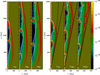 |
Fig. 10 Density maps for the no-DW reference simulation (three frames on the left) and the DW simulation (three frames on the right) at t = 71, 119, and 167 yr. The white contours indicate the surface of 50% (solid line) and 90% (dashed line) jet material mixing fractions. The black lines in the disk-wind simulation show a cone of α = 11° opening half-angle, which circumscribes the boundary the region perturbed by the jet and its IWS. The black dashed lines show the predicted trajectory of the edge of the bow shock (see Eq. (14)). The density color scale is given by the right bar (in g cm−3). |
In the no-DW simulation, the region perturbed by the jet behind the leading bowshock expands into a roughly cylindrical shape, which tapers off close to the position of the outflow source (where it becomes a weak, radially expanding shock). This is the standard shape of the perturbed region in simulations of variable, radiative jets propagating into a uniform static medium, seen since the early work of Stone & Norman (1993) and Biro & Raga (1994).
In the disk wind simulation, in contrast, the region perturbed by the jet behind the leading bowshock takes a conical shape, tapering off at large distances from the outflow source. For the parameters of our DW simulation, the half-opening angle of the perturbed region is α ≈ 11° (see Fig. 10). This cone is located outside the predicted trajectory of the edge of the bow shock (drawn in black dashed line) given by Eq. (14). This broadening occurs because, as discussed in item 3 of Sect. 3.2.2, the edge of the bow shock drives a weak outer shock into the undisturbed DW, which propagates away at a speed close to cs ∼ .8 km s−1. Taking into account the advection of the weak shock by the DW, one predicts that this will broaden the disturbed region by an angle ß = arctan cs/vw = 4°, in agreement with the observed cone opening. Obviously, in the no-DW simulations, this weak outer shock travels laterally without being advected, and no limiting cone forms.
In this surprisingly simple configuration adopted by our jet + disk wind simulation, the overall long-term effect of the disk wind is to stop the perturbations from travelling beyond this “opening cone” of the sideways ejection from the IWS. Another important effect of the DW is to push the locus of 50 % ambient material (white contour) closer to the jet axis than in the no-DW case, due to the disk wind partial refilling behind each bowshock. Hence, the first few IWS close to the source can still sweep up (possibly molecular) DW material. The internal IWS are also more curved than in the no-DW case, where material ejected sideways meets a very low-density cocoon, producing flat-topped internal bowshocks (see Fig. 10).
4. Summary
In this paper we have presented a first exploration of an hydrodynamical flow composed by an inner, variable jet surrounded by a slower, steady, cylindrical disk wind. The jet variability produces IWS which drive bow shocks into the disk wind, producing a strong coupling between the two components of the flow.
We have developed a standard thin shell model for the bow shock driven into the disk wind by a single IWS, for a jet of arbitrarily small radius (see Sect. 2), deriving the shape of the bow shock and the refilling by the continuing disk wind of the cavity left behind by the bow shock. The model was extended
to give a qualitative description of the flow resulting from two or more successive IWS bow shocks plowing through the disk wind (Sect. 3).
The appropriateness and limitations of the predictions of bow shock shapes and kinematics from this analytic model have been checked with axisymmetric numerical simulations: one of a variable jet + disk wind configuration, and a second reference simulation with the same variable jet surrounded by a stationary environment. We compared the analytic model with the numerical simulations, and we found a relatively good agreement, giving us an understanding of the main features of the simulated flows. These features are:
-
the bow shocks of the numerical IWS have cubic morphologies which can be reproduced quite convincingly with the thin-shell, momentum conserving analytic model (see Eqs. (10) and (11) and Fig. 6);
-
the kinematics in the simulated bow shocks has a behavior which approximately follows the kinematics predicted from the analytic model for the fully-mixed layer (for jetdominated material) or the immediate post-bow shock gas (for high-pressure swept-up ambient gas) (see Figs. 4 and 9);
-
these bow shocks leave behind cavities which are partially refilled by the slower disk wind (see Figs. 3 and 8);
-
thanks to this refilling, subsequent IWS will propagate into fresh disk wind material up to a distance from the source lc= Δz/(vj/vw –1) (see Figs. 5 and 10).
The main contribution of this paper is thus to provide a numerically validated, simple analytic model which can be used to model bow-like shapes of knots observed close to the outflow sources in high velocity, collimated optical and molecular outflows (Lavalley-Fouquet et al. 2000; Podio et al. 2015). As shown by our simulations, this shape modeling (in the narrow jet limit) allows one to estimate the sideways ejection velocity from the IWS and the length scale of the bow-shock. From this, constraints could be inferred on the mass-loss rate from the IWS and the surrounding flow properties (see Eq. (6)).
Another important contribution of this paper is to predict the regions where a surrounding disk wind would remain unperturbed. A quite dramatic result of our jet + disk wind simulation is that the perturbations of the disk wind by the IWS bow shocks are confined inside a cone. Therefore, all of the gas outside this confinement cone is unperturbed disk wind material. Also, there are pockets of undisturbed disk wind material within this cone, in the refilled region between the source and the last IWS, and also ahead of the latest IWS when it is at z < lc (see the three right hand frames of Fig. 10). These are the regions in which one still finds a record of the undisturbed characteristics of the disk wind, which could be useful for comparisons with disk wind models.
Finally, another result of observational interest is that we identify several distinctive signs of a cylindrical DW around a time-variable jet: (i) bow shocks that close upon the axis at a finite distance from the source (at a fraction vw/vj of the distance to the bow apex), (ii) a non-zero (= vw) asymptotic value of longitudinal velocity in the far bowshock wings, (iii) internal bowshocks that are curved rather than flat-topped, (iv) a predominance of DW material ahead of the first few IWS, which (if the DW is chemically richer and/or dustier than the jet) should produce different emission signatures compared to the more distant IWS.
Extensions of the analytic model to more complex jet + disk wind flows do not appear very attractive (as, e.g., relaxing the assumption of a cylindrical uniform disk wind) as quite complex expressions are obtained, and are therefore not straightforwardly applicable to model observed structures. On the other hand, the numerical simulations presented here can be extended in many directions, including a more realistic disk wind model (e.g., with a radial dependence of the density and velocity, and a velocity not aligned with the outflow axis); studying the effect of a non-top hat jet cross section; going from the HD to the MHD equations; including a chemical/ionic network and the associated cooling functions. If future comparisons between jet + disk wind models and observations are sufficiently promising, the extensions listed above (as well as other easily imagined possibilities) will become worthy of exploration.
Acknowledgments
We thank the anonymous referee for useful comments. This work has been done within the LABEX PLAS@PAR project, and received financial state aid managed by the Agence Nationale de la Recherche, as part of the “Programme d’Investissements d’Avenir” under the reference ANR-11-IDEX- 0004-02. AR acknowledges support from the DGAPA (UNAM) grant IG100218. This research has made use of NASA’s Astrophysics Data System.
Appendix A: General equations
In the analytic part of this work, equations ruling the geometry and the kinematics of a bow shock travelling in a disk wind are given for simplicity in the narrow jet limit rj → 0. In this appendix, we give equations valid for an arbitrary jet width that we have used to fit numerical simulations. For the definition of the quantities, we refer to Figs. 1 and 2.
A.1. Shape of the bow-shock and of the cavity
Eqs. (1) to (8) are valid for an arbitrary width of a jet. Inserting zb = zj – x into Eq. (5) we get the shape of the bow shock (zb, rb) (see thick cyan line Fig. 1): (A.1)
(A.1)
Eq. (8) gives straightforwardly the radius rbf of the edge of the bow shock shell![Mathematical equation: $$ \frac{1}{\gamma {L}_0^2}\left[{r}_{b,f}^3-{r}_j^3+3{r}_j^2({r}_j-{r}_{b,f})\right]+{r}_{b,f}-{r}_j={v}_0t={z}_j\frac{{v}_0}{{v}_j}, $$](/articles/aa/full_html/2018/06/aa32031-17/aa32031-17-eq37.gif) (A.2)
(A.2)
Combining Eqs. (A.1) and (A.2) we get the trajectory of the outer edge of the cavity (black dotted line Fig. 1): (A.3)
(A.3)
The boundary of the partially refilled cavity (cyan dash-dotted line Fig. 1) obtained from Eqs. (A.2) and (A.3) is given by: (A.4)
(A.4)
Hence, in the wide jet case, the boundary between the refilled region and the empty cavity has a conical shape.
A.2. Kinematics
Integration of Eqs. (1)–(3) gives the fully mixed radial and axial velocities: (A.5)
(A.5)
 (A.6)
(A.6)
Immediate post-shock velocities obtained by considering the velocity component tangential to the shock surface are: (A.7)
(A.7)
 (A.8)
(A.8)
The flat UV flux in their UV1–UV2 models is ~30–500 that in BP Tau (Bergin et al. 2003), for a wind-mass flux corresponding to a 1000 times larger accretion rate (~3 × 10⁻⁵ Mʘ yr−1).
Noting that L0 is the radius where the swept-up x-momentum is equal to 3 times the injected r-momentum ṁ0 v0, Eq. (5) is equivalent to Eq. (22) in Ostriker et al. (2001).
References
- Bergin, E., Calvet, N., D’Alessio, P., & Herczeg, G. J. 2003, ApJ, 591, L159 [NASA ADS] [CrossRef] [Google Scholar]
- Biro, S., & Raga, A. C. 1994, ApJ, 434, 221 [NASA ADS] [CrossRef] [Google Scholar]
- Blondin, J. M., Fryxell, B. A., & Konigl, A. 1990, ApJ, 360, 370 [NASA ADS] [CrossRef] [Google Scholar]
- Cabrit, S. 2002, in Proceedings of “Star Formation and the Physics of Young Stars”, eds. J. Bouvier & J.-P. Zahn (Les Ulis, Fr: EDP Sciences), EAS Pub. Ser, 3, 147 [Google Scholar]
- Cabrit, S., Codella, C., Gueth, F., et al. 2007, A&A, 468, L29 [NASA ADS] [CrossRef] [EDP Sciences] [Google Scholar]
- Claussen, M. J., Marvel, K. B., Wootten, A., & Wilking, B. A. 1998, ApJ, 507, L79 [NASA ADS] [CrossRef] [Google Scholar]
- de Gouveia dal Pino, E. M., & Benz, W. 1993, ApJ, 410, 686 [Google Scholar]
- Dougados, C., Cabrit, S., Lavalley, C., & Ménard, F. 2000, A&A, 357, L61 [NASA ADS] [Google Scholar]
- Ellerbroek, L. E., Podio, L., Kaper, L., et al. 2013, A&A, 551, A5 [NASA ADS] [CrossRef] [EDP Sciences] [Google Scholar]
- Falle, S. A. E. G. 1991, MNRAS, 250, 581 [NASA ADS] [CrossRef] [Google Scholar]
- Glassgold, A. E., Mamon, G. A., & Huggins, P. J. 1991, ApJ, 373, 254 [NASA ADS] [CrossRef] [Google Scholar]
- Hartigan, P., Raymond, J., & Hartmann, L. 1987, ApJ, 316, 323 [NASA ADS] [CrossRef] [Google Scholar]
- Hodapp, K. W., & Chini, R. 2014, ApJ, 794, 169 [NASA ADS] [CrossRef] [Google Scholar]
- Lavalley-Fouquet, C., Cabrit, S., & Dougados, C. 2000, A&A, 356, L41 [NASA ADS] [Google Scholar]
- Lee, C.-F., Stone, J. M., Ostriker, E. C., & Mundy, L. G. 2001, ApJ, 557, 429 [NASA ADS] [CrossRef] [Google Scholar]
- Lee, C.-F., Ho, P. T. P., Li, Z.-Y., et al. 2017, Nat. Astron., 1, 0152 [NASA ADS] [CrossRef] [Google Scholar]
- Matt, S., & Pudritz, R. E. 2005, ApJ, 632, L135 [NASA ADS] [CrossRef] [Google Scholar]
- Ostriker, E. C., Lee, C.-F., Stone, J. M., & Mundy, L. G. 2001, ApJ, 557, 443 [NASA ADS] [CrossRef] [Google Scholar]
- Panoglou, D., Cabrit, S., Pineau Des Forêts, G., et al. 2012, A&A, 538, A2 [NASA ADS] [CrossRef] [EDP Sciences] [Google Scholar]
- Podio, L., Codella, C., Gueth, F., et al. 2015, A&A, 581, A85 [NASA ADS] [CrossRef] [EDP Sciences] [Google Scholar]
- Raga, A., & Cabrit, S. 1993, A&A, 278, 267 [Google Scholar]
- Raga, A. C., & Canto, J. 1989, ApJ, 344, 404 [NASA ADS] [CrossRef] [Google Scholar]
- Raga, A. C., Binette, L., Canto, J., & Calvet, N. 1990, ApJ, 364, 601 [NASA ADS] [CrossRef] [Google Scholar]
- Raga, A. C., Williams, D. A., & Lim, A. J. 2005, Rev. Mex. Astron. Astrofis., 41, 137 [Google Scholar]
- Raymond, J. C., Cox, D. P., & Smith, B. W. 1976, ApJ, 204, 290 [NASA ADS] [CrossRef] [Google Scholar]
- Romanova, M. M., Ustyugova, G. V., Koldoba, A. V., & Lovelace, R. V. E. 2002, ApJ, 578, 420 [NASA ADS] [CrossRef] [Google Scholar]
- Shu, F., Najita, J., Ostriker, E., et al. 1994, ApJ, 429, 781 [NASA ADS] [CrossRef] [Google Scholar]
- Stone, J. M., & Norman, M. L. 1993, ApJ, 413, 198 [NASA ADS] [CrossRef] [Google Scholar]
- Tabone, B., Cabrit, S., Bianchi, E., et al. 2017, A&A, 607, L6 [NASA ADS] [CrossRef] [EDP Sciences] [Google Scholar]
- Tafalla, M., Myers, P. C., Mardones, D., & Bachiller, R. 2000, A&A, 359, 967 [NASA ADS] [Google Scholar]
- Toro, E. F. 1999, Riemann solvers and numerical methods for fluid dynamics: a practical introduction (Berlin: Springer) [CrossRef] [Google Scholar]
- White, M. C., Bicknell, G. V., Sutherland, R. S., Salmeron, R., & McGregor, P. J. 2016, MNRAS, 455, 2042 [NASA ADS] [CrossRef] [Google Scholar]
- Yvart, W., Cabrit, S., Pineau des Forêts, G., & Ferreira, J. 2016, A&A, 585, A74 [Google Scholar]
- Zanni, C., & Ferreira, J. 2013, A&A, 550, A99 [NASA ADS] [CrossRef] [EDP Sciences] [Google Scholar]
All Tables
All Figures
|
Fig. 1 Schematic diagram of the flow around an internal working surface (IWS) in the frame of reference co-moving with the IWS at velocity vz = vj (a similar configuration would apply for the leading working surface of a jet). The thick, horizontal line at the bottom of the graph is the jet (with a gap showing the position of the IWS). The working surface ejects jet material sideways at an initial velocity v0 into the slower disk wind, which in this frame of reference moves towards the outflow source at velocity vj – vw. The distance x is measured towards the outflow source.The shape of the thin shell bow shock is given by rb(x) (see Eq. (5)), and terminates at the cylindrical radius rb; f(t) with t the time elapsed since formation of the IWS (see Eq. (8)). |
| In the text | |
|
Fig. 2 Schematic diagram showing the flow around a working surface of a jet (in this case the leading working surface, but the diagram also applies for an internal working surface). The jet is the horizontal, red rectangle at the bottom of the graph, with the source located at z = 0. The working surface in yellow is located at a distance zj from the source and travels at a velocity vj. It ejects material away from the axis at an initial velocity v0. The jet is surrounded by a “disk wind”, which travels along the outflow axis at a velocity vw. The shape of the thin-shell bow shock (thick cyan line) is given by zb as a function of r and ends at the edge of the bow wing (cyan point; zb f, rb f). The bow shock leaves behind a “cavity” (black region), which is partially refilled by the disk wind (brown region). The boundaries of the initial swept up cavity (in black dashed line) and of the refilled region (cyan dash-dotted line) are given by zf an zc (respectively) as a function of cylindrical radius r (see Eqs. (14) and (15)). |
| In the text | |
|
Fig. 3 Time evolution of the bow shock + cavity flow predicted by the analytic model for two choices of the wind velocity: vw = 0 (leftframe) and vw = 0.4vj (right frame). The dark region is the empty part of the cavity (swept-up in the thin shell bow shock) and the brown region is the part of the cavity that has been refilled by the disk wind (this region being of course absent in the vw = 0 model of the left frame). For both models, we show snapshots corresponding to t = 2L0/Vj, 4L0/Vj, and 8L0/vj), which result in positions zj = 2L0, 4L0, and 8L0 for the working surface (see the labels on the top left of each frame). Both models have v0 = 0.2vj |
| In the text | |
|
Fig. 4 Shape of the bow shock and the cavity (top), radial velocities vr (center) and axial velocities vz (bottom) for the two models discussed in the text. The solid curves show the velocities of the well-mixed material within the thin shell flow, and the dashed curves show the immediate post-bow shock velocities. The dotted red line shows vz = vw. |
| In the text | |
|
Fig. 5 Time evolution of two successive bow shocks and the cavities predicted by the analytical model. The first bow shock is ejected at t = 0, the second shock is formed at time t = τj when the first bow shock is at z = vjτj taken here as 6L0 (top). At a time t = τj + 2L0/vj, the second bow shock is still propagating in the undisturbed disk wind material (center). At a time tc the second bow shock catches up the emptied cavity of the first bow shock at its vertex (bottom). |
| In the text | |
|
Fig. 6 Maps of density and pressure for the reference no-DW simulation with vw = 0 (left) and the DW simulation with vw = 0.4vj(right) at a time t = 48 yr. Color scales on top are in g cm−3 for density and in dyn cm−2 for pressure. White contours show the locus of 50% mixing ratio between jet and disk-wind/ambient material. The cyan curve shows a fit (to the numerical results) by the analytic shell shape in Eq. (11), with L0 = 65 au (left) and 108 au (right). The cyan dot indicates the maximum radius of the shell, the cyan asterix indicates the predicted vertex of the empty conical cavity left behind the shell, and the cyan dash-dotted line is the analytical predicted boundary between the emptied cavity and the region refilled from below by fresh disk wind (see Fig. 2 and Eq. (15)). |
| In the text | |
|
Fig. 7 Transverse cut across the flow at the IWS location (z = 993 au) in the no-DW time-frame shown in Fig. 6. This cut shows the radial velocity as a function of distance from the jet axis in solid line. We also plot the radial velocity weighted by the abundance of the jet tracer with a dashed line. The radial velocity first grows outwards, reaches a maximum velocity of ≈ 14 km s−1 at a radius of ∼ 25 au (somewhat larger than the 20 au initial jet radius), and then remains with values > 10 km s−1 until it drops sharply to 0 at r ∼ 50 au. The velocity maximum at r ∼ 25 au corresponds to the shock against the jet material. The second maximum at r ∼ 50 au is the shock that propagates in the disk-wind and the zero radial velocity material at larger radii is the undisturbed disk wind. |
| In the text | |
|
Fig. 8 Zoom of the leading IWS of the simulation with a surrounding disk wind at time t = 48 yr. Left: density stratification (with the logarithmic color scale given by the top bar in g cm−3), center: radial velocity (with the linear scale of top bar in km s͔–1) and right: axial velocity structure (with the linear scale of the top bar in km s−1). The white contours show the surfaces of 50 % (solid line), 10 %, 0.1 % and 0.001 % (outer contour) jet material mixing fractions. The cyan asterisk is the predicted vertex of the cavity, the cyan dash-dotted line in the predicted boundary of the cavity, and the cyan curve is the fitted shape of the bow shock. |
| In the text | |
|
Fig. 9 Longitudinal position-velocity (PV) diagrams for the no DW simulation (top) and the DW simulation (bottom). From left to right: vr for the jet material only, vr for the surrounding material only, vz for the jet material only, vz for the surrounding material only, and density stratification. The ordinate of all frames is position along the outflow axis (in au). The color scale in the PVs is scaled by volume × cube of pressure so as to be maximum (in red and yellow shades) for shocked material in the shell, while the color scale for density is in g cm−3. Blue curves are predicted velocities in the full mixing hypothesis (Eqs. (16) and (17)), while magenta curves are the predicted immediate-post shock velocities (Eqs. (18) and (19)). |
| In the text | |
|
Fig. 10 Density maps for the no-DW reference simulation (three frames on the left) and the DW simulation (three frames on the right) at t = 71, 119, and 167 yr. The white contours indicate the surface of 50% (solid line) and 90% (dashed line) jet material mixing fractions. The black lines in the disk-wind simulation show a cone of α = 11° opening half-angle, which circumscribes the boundary the region perturbed by the jet and its IWS. The black dashed lines show the predicted trajectory of the edge of the bow shock (see Eq. (14)). The density color scale is given by the right bar (in g cm−3). |
| In the text | |
Current usage metrics show cumulative count of Article Views (full-text article views including HTML views, PDF and ePub downloads, according to the available data) and Abstracts Views on Vision4Press platform.
Data correspond to usage on the plateform after 2015. The current usage metrics is available 48-96 hours after online publication and is updated daily on week days.
Initial download of the metrics may take a while.