| Issue |
A&A
Volume 614, June 2018
|
|
|---|---|---|
| Article Number | A105 | |
| Number of page(s) | 19 | |
| Section | Extragalactic astronomy | |
| DOI | https://doi.org/10.1051/0004-6361/201731688 | |
| Published online | 21 June 2018 | |
Multi-scale simulations of black hole accretion in barred galaxies
Self-gravitating disk models
1
Institute for Theoretical Physics and Astrophysics, Kiel Astrophysics, Christian-Albrechts-University Kiel,
Leibnizstraße 15,
24118
Kiel, Germany
2
Hamburger Sternwarte, Universität Hamburg,
Gojensbergweg 112,
21029
Hamburg, Germany
e-mail: manuel.jung@hs.uni-hamburg.de
3
Steward Observatory, The University of Arizona,
Tucson
AZ
85721, USA
Received:
1
August
2017
Accepted:
18
February
2018
Due to the non-axisymmetric potential of the central bar, in addition to their characteristic arms and bar, barred spiral galaxies form a variety of structures within the thin gas disk, such as nuclear rings, inner spirals, and dust lanes. These structures in the inner kiloparsec are extremely important in order to explain and understand the rate of black hole feeding. The aim of this work is to investigate the influence of stellar bars in spiral galaxies on the thin self-gravitating gas disk. We focus on the accretion of gas onto the central supermassive black hole and its time-dependent evolution. We conducted multi-scale simulations simultaneously resolving the galactic disk and the accretion disk around the central black hole. In all the simulations we varied the initial gas disk mass. As an additional parameter we chose either the gas temperature for isothermal simulations or the cooling timescale for non-isothermal simulations. Accretion was either driven by a gravitationally unstable or clumpy accretion disk or by energy dissipation in strong shocks. Most of the simulations show a strong dependence of the accretion rate at the outer boundary of the central accretion disk (r < 300 pc) on the gas flow at kiloparsec scales. The final black hole masses reach up to ~109 M⊙ after 1.6 Gyr. Our models show the expected influence of the Eddington limit and a decline in growth rate at the corresponding sub-Eddington limit.
Key words: hydrodynamics / galaxies: structure / accretion, accretion disks / quasars: supermassive black holes / galaxies: spiral / black hole physics
© ESO 2018
1 Introduction
Recent very high-resolution observations (~100 pc) have given the first insights into the inner structures of barred spiral galaxies and reveal the circumnuclear disk, nuclear spirals, and rings, which are often subject to high star formation rates (Xu et al. 2015; Fathi et al. 2015; Salak et al. 2016). These efforts gradually increase our knowledge about this kind of galaxies on which detailed models can be built. Despite these improvements we still lack a consistent picture of the angular momentum transport mechanisms and the feeding of the central supermassive black hole. In case of active galactic nuclei (AGN), measurements of the nuclear luminosity and the bulge velocity dispersion allowed us to make a connection between the black hole and the bulge early on (Ferrarese & Merritt 2000; Gebhardt et al. 2000; McConnell et al. 2011). While an explanation for this connection is still highly debated, the importance of multiple different heating and cooling processes such as star formation, supernova explosions, and AGN feedback cannot be neglected. An excellent review highlighting the various aspects of black hole growth can be found in (Alexander & Hickox 2012).
In the last 20 yr there have been great efforts to include different effects of the energy balance in galaxies. In regions with high star formation rates the starlight can heat the gas (Stinson et al. 2006; Christensen et al. 2010), and the stars rapidly explode as supernovae and inject momentum and energy into the interstellar medium (Yepes et al. 1997; Scannapieco et al. 2008; Murante et al. 2010). Also, there have been efforts to include the observed multi-phase medium into the models (Springel & Hernquist 2003; Braun & Schmidt 2012). All of these simulations are based on the smoothed particle hydrodynamics (SPH) method (Gingold & Monaghan 1977; Lucy 1977). Resolving a self-gravitating accretion disk in the central nuclear region (<300 pc) with the SPH method is difficult. Although this region can have a high gas density, it contributes only 2% to the overall mass of the gaseous disk. Thus, the number of SPH particles in this region will only be about 2% of all particles. Achieving a high number of neighbor particles and high resolution in this region would require spending most particles on out-of-focus regions.
There have been attempts to cover multi-scale gas behavior by stopping and restarting the simulation at a higher resolution (Hopkins & Quataert 2010), but ultimately high resolution in the central region can only be achieved with grid-based methods. Because of the high velocities near the black hole and the inclusion of self-gravity, this is very computationally expensive even in 2D.
Several 2D simulations of barred galaxies have been carried out before. Early simulations were focused on the large-scale structures (e.g., density waves) and their dependence on pattern speeds (Berman et al. 1979; Sellwood & Sparke 1988; Lindblad et al. 1996). Athanassoula (1992) discussed the dependence of the shape and position of dust lanes on general galaxy parameters (e.g., the bar parameter) and found substantial inflow in models with strong shocks. Later Athanassoula (2000) confirmed these findings andbriefly discussed the role of a secondary bar inside of the main one. In addition, Maciejewski et al. (2002) examined the role of secondary bars and found that they cannot generate shocks in the gas flow, which would be visible inobservations and are unlikely to increase mass inflow into the galactic nucleus. The curvature of the dust lanes is determined by Comerón et al. (2009) and they deduce that it is predominantly a result of the parameters of the bar. Sormani et al. (2015a) investigate the gas streamlines for different orbit families in detail and find for sufficiently high sound speeds and resolution that the flow downstream of the shocks becomes unsteady.
The main focus of most publications has been on nuclear structures like nuclear rings and spirals. The generation and position of nuclear rings was analyzed by Piner et al. (1995) and they found a connection to the inner Lindblad resonance position. Regan & Teuben (2003) disagreed and provided a model in which they are not related to inner Lindblad resonances as was previously thought. Namekata et al. (2009) discuss the impact of nested bars on the gas inflow and find that a nuclear self-gravitationally unstable gas disk is generated for some simulation setups. Kim et al. (2012b) survey the dependencies of the structure of nuclear rings and spirals to the sound speed and the mass of a central black hole. Sormani et al. (2015c) vary the quadrupole of the bar potential and compare it to the longitude–velocity diagram of the Milky Way to constrain bar parameters. Li et al. (2015) distinguish between round and elongated nuclear rings and identify global parameters, which correlate with the position of round rings.
Several publications are dedicated to the effects of bar strengths. Regan & Teuben (2004) find that weak bars have almost no effect on the radial distribution of the gas, but strong bars can drive gas down to the nuclear ring, but not any further. Kim et al. (2012a) investigate the complicated dependencies of nuclear structures on different bar strengths. The large-scale formation of the spiral arms emerging from the ends of galactic bars are examined by Sormani et al. (2015b). They find that they can be understood as kinematic density waves.
Magnetic fields can enhance the mass influx rate driven by shocked gas in dust lanes. Eventually a magnetic dynamo outside of the corotation resonance radius can turn the outer disk into a highly chaotic state (Kim & Stone 2012; Kim 2013). Star formation in nuclear rings, which is solely fueled by gas inflow as the result of a bar potential (which was examined by Seo & Kim 2013; Kim et al. 2014b) occurs mainly at the connection point between nuclear ring and dust lanes. The star formation rate correlates with the mass inflow rate to the ring, but not with the mass of the ring.
In this work we focus on the black hole accretion flow and extend the simulation domain to the subparsec scale. We also account for self-gravity of the gas.
In the second part of this paper we eliminate the restriction on isothermal models. We account for the contribution of shock and compressional heating and a simple one-parameter cooling depending only on the orbital timescale are considered. The selection of the cooling parameter in this connection is based on the critical value of bcool (Gammie 2001), which is known to produce marginal stable accretion disk flows in these systems. This is also justified by the observations of Fathi et al. (2015), who give an estimate for the Toomre parameter (Toomre 1964) of NGC 7469, from which follows that the inner region should be gravitationally unstable. These models are also the first steps toward more detailed models of the heating and cooling effects, among others, include stellar radiation feedback, star formation feedback, and supernova explosions, which is the scope of future work.
In the first paper (Jung et al. 2018; hereafter Paper I) we established the numerical foundation to execute isothermal multi-scale simulations of black hole accretion in barred galaxies. To do this, we introduced a method for conserving inertial angular momentum in a rotating reference frame, a spectral self-gravity solver and discussed the importance of the gravitational energy transport in the energy equation. These extensions are crucial in order to accurately simulate the accretion onto the central black hole, which is significantly determined by the angular momentum transport processes within the disk, and is the subject of this paper.
The paper is structured as following. In Sect. 2 we present the model of a self-gravitating gas disk subject to multiple gravitational potentials. In Sect. 3 we present our isothermal simulation results and classify them in a strong and a weak accretion mode. In Sect. 4 we outline the results from the simulations with cooling, and classify them in a hot and cold accretion mode. In Sect. 5 we present our conclusions.
2 Model
2.1 Gravitational potentials
The most important part of all following galaxy simulations is the implementation of the gravitational potential. The set of potentials applied in this work is basically that given in Kim et al. (2012b), although we modified their implementation by adding a Newtonian point mass potential for the black hole and relaxing the razor thin disk approximation for the stellar disk potential. The parameters in the gravitational potentials are chosen to be similar to Piner et al. (1995) and Kim et al. (2012b), thus a typical flat galaxy rotation profile is recovered.
Black hole: The black hole is modeled by a Newtonian point mass potential:
 (1)
(1)
The inner boundary of the simulation domain is far enough away to neglect any relativistic effects. The initial mass of the black hole MBH = 106 M⊙ is allowed to grow during the simulation. The mass flux across the inner boundary is calculated at each time step, which sometimes yields super-Eddington accretion rates. In that case we limit the actual black hole accretion rate ṀBH to at most the Eddington rate ṀEdd (Davis & Laor 2011). At each time step Ṁacc is calculatedand the Eddington limited result of this is added to the black hole mass:
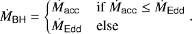 (2)
(2)
If the accretion rate is greater than the Eddington limit, the excess mass is removed from the system. We call this Eddington outflow:
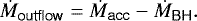 (3)
(3)
While feedback by the Eddington outflow is not considered in these simulations, radiation pressure onto the gas disk is negligible since the disk is geometrically thin. A feedback by the black hole spin is part of the black hole accretion efficiency factor η (Davis & Laor 2011).
Stellar disk: The stellar disk is approximated by a Kuzmin–Toomre model (Kuzmin 1956; Toomre 1963; Binney & Tremaine 2008) for the stellar density, which is given by
 (4)
(4)
The corresponding midplane potential is
 (5)
(5)
with the constants R0 = 14.1 kpc and R1 = 14.1 pc. The total disk mass amounts to
 (6)
(6)
with v0 = 260 km s−1.
Bulge: The bulge is modeled by a modified spherically symmetric Hubble profile (Binney & Tremaine 1987) of the density
 (7)
(7)
resulting in the potential
 (8)
(8)
The density is  and the characteristic extension Rb = 0.33 kpc. The mass inside of a 6 kpc radius of the bulge amounts to Mbul = 2.8 × 10¹⁰M⊙.
Bar: The bar potential is modeled using a Ferrers potential (Ferrers 1887; Chandrasekhar 1969; Pfenniger 1984) for the stellar density
 (9)
(9)
with g = x2a2 + y2b2 + z2c2; a the major and b, c the minor semi-axes respectively. The Ferrers potential can be used for a general ellipsoid, if specifying the third semi-axis length c≠ b. We set in these simulations c = 0.99b since the Ferrers potential is only defined for c < b, but we want to achieve approximately a prolate spheroid. The fourth parameter n in the exponent controls the decline of the density. We set for all the simulations in this paper n = 1, a = 5 kpc, b = 2 kpc, and  . The total mass of the bar is Mbar = 1.5 × 10¹⁰M⊙. The midplane bar potential is
 (10)
(10)
using the definition of the potential and its coefficients Wijk from Pfenniger (1984). The coefficients are repeated in Appendix A. The bar potential is slowly switched on during the first rotation of the bar, so that a violent adoption of the gas surface density can be prevented. To suppress radial perturbations entirely, we keep the total system mass constant. The initial bulge mass is the sum of the intended bulge and bar masses. During the switch-on phase mass is removed from the bulge at the same rate as it is added to the bar (Kim et al. 2012b). Therefore, the rotation law as well as the balance of centrifugal force and radial gravitational forces remain unchanged. The bar rotates withthe angular velocity
 (11)
(11)
Since a rotating frame of reference is used with an angular velocity of Ωp, the bar rests in all simulations along the x-axis.
All of these potentials model the gravitation of stars, dark matter, and of a black hole. In addition to the discussed gravitational components, we allow for self-gravitation (Chan et al. 2006; Li et al. 2009). Hereafter we use the delta distribution as Green function to model a razor thin gas disk.
2.2 Initial and boundary conditions
In the simulations we consider the gas component as the vertically integrated surface density Σ. The disk is discretized as a mesh in polar coordinates using a logarithmic radial scaling. The radial extent spans R ∈ [2 pc, 16 kpc]. The mesh resolution is Nr × Nφ = 384 × 256, which amounts to an aspect ratio of ~1 within each cell and to a cell size Δx of 0.05 pc, 0.25 pc, and 25 pc at 2 pc (inner rim), 10 pc, and 1 kpc, respectively.Due to the logarithmic radial scaling, half of the radial cells resolve the inner accretion disk r < 300 pc, which is the most important region for the accretion flow. We trade some overall resolution to cover for the extended cost and number of shorter time steps, because of the increased demands of the CFL criterion (Courant et al. 1928) in connection with the small cells at the inner boundary to ensure numerical stability, very long simulation run times and self-gravity. One simulation leverages about two weeks of real time on the provided NEC SX ACE vector super computer. This amounts to 8064 CPU hours for each simulation setup, which is roughly equivalent to 130 000 CPU hours on Intel Xeon E5-2670 CPUs.
The initial surface density follows a power law with an exponent κ = −1, which is limited near the inner boundary:
 (12)
(12)
The cutoff radius is Rκ = 100 pc and the initial mass Σ0 is a parameter of the model space. With this cutoff radius we achieve similar mass densities at R = 1 kpc as in Kim et al. (2012b). A power law with negative exponent is necessary for the surface density, because otherwise a local minimum of the gravitational potential, generated by the self-gravitation, would lead to non-physical solutions. Illenseer & Duschl (2015) describe in detail which power laws are sensible choices for accretion disks. Our choice for the power law and the initial density generate densities at radius Rκ, which are comparable to those generated in Kim et al. (2012b). To excite any potentially existing instabilities, we add a noise on the order of 10−3 to the surface density distribution. Table 1 summarizes the initial mass of all gravitational sources.
At the beginning of the simulation the radial velocity field is zero and the azimuthal velocity is chosen so that the centrifugal force is balanced by all other forces, i.e., gravitational and pressure gradient forces. Numerically, this is achieved by evaluation of the right-hand side of the system of differential equations, which consists of all source terms and the flux difference quotients. This is important because generally it will deviate from the analytic term by means of the numerical flux calculation and linear reconstruction. A more detailed explanation can be found in Paper I. The resulting rotation curve shows the typical flat slope at large radii (see van Albada et al. 1985). The difference to curves for simulations of different total gas mass and therefore stronger self-gravitation is negligible. The gas rotates in the mathematical positive direction, i.e., in the rotating reference frame within (beyond) the corotation radius counterclockwise (clockwise).
At the outer boundary we use a no-gradients condition. At the inner boundary we set an outflow condition and extrapolate the azimuthal velocity with a Keplerian profile to prohibit gas inflow into the computational domain. In general when simulating accretion disks one has to choose how to extrapolate the specific angular momentum in the boundary cells. While a no-gradients boundary condition is often chosen as an approximation at the inner boundary, it can induce a torque into the inner disk that can alter the flow significantly. According to our experience a Keplerian extrapolation introduces no noteworthy torque into the inner disk. Strictly speaking an inner Kepler boundary condition is only a good approximation if the rotation profile in a few cells next to the inner boundary is also Keplerian during the entire simulation time. In particular, this requires an initially non-self-gravitating inner accretion disk, otherwise the surface density distribution would dictate a non-Keplerian rotation profile. However, without a density cutoff the mass of the disk r < 100 pc would approach an overall mass on the order of the initial black hole mass (106 M⊙) and has to be considered self-gravitating. At the same time Σ0 is fixed sincethe surface density at 1 kpc should be comparable to the value of Kim et al. (2012a). All the simulations in this paper indeed show a rotation profile in a few cells next to the inner boundary, which is close to Keplerian throughout the complete simulation time.
One rotation of the bar and the orbital periods at the inner and outer boundary last respectively
 (13)
(13)
The simulation stop time is after nine bar rotations
 (14)
(14)
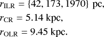
Lindblad resonances are important for the dynamics of the system (Lin & Shu 1964, 1966; Binney & Tremaine 2008). Figure 1 shows their dependencies on the initial resonant frequencies and the bar angular velocity for one of the simulations. At the beginning this structure is very similar in all the simulations because all the gravitational potentials remain the same except for the contribution from the self-gravitating disk. The locations of the inner and outer Lindblad resonances, rILR and rOLR, respectively, as well as the corotation resonance rCR are given by
 (15)
(15)
A constant speed of sound is defined for the isothermal simulations in the entire calculation domain, which is thesecond parameter of the model space. If we assume an ideal, completely ionized gas consisting of 75% hydrogen and 25% helium, the equation of state is given by
 (16)
(16)
where the mean molecular weight can be specified as μ = 6.02 × 10⁻⁴ kg mol−1 (Kippenhahn & Weigert 1990). The temperature is then a function of gas density and pressure:
 (17)
(17)
Here RG identifies the universal gas constant. The isothermal equation of state
 (18)
(18)
is used for the isothermal simulations. Therefore, in this case the temperature is a function of the isothermal sound velocity
 (19)
(19)
Summary of the initial masses of the different gravitational components and initial surface density parameters.
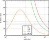 |
Fig. 1 Frequency distribution curves of the inner Lindblad (ILR), outer Lindblad (OLR), and corotation (CR) frequency. The horizontal line is the bar frequency Ωp. The intersections of these curves are resonance loci. |
2.3 Non-isothermal extensions
For the non-isothermal simulations, we use the parameterized cooling function proposed by Gammie (2001). It is based on the coupling of the cooling timescale τcool to the dynamical timescale τdyn by the dimensionless parameter bcool
 (20)
(20)
Using the internal energy e = p∕(γ − 1) and the azimuthal angular velocity Ω the cooling source term Scool becomes
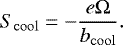 (21)
(21)
Irrespective of hydrodynamic heating processes (e.g., shock and compressional heating), we model no further heating mechanisms. In addition, gas in spiral galaxies can be heated by star formation and the resultant stellar winds and supernovae (McKee & Ostriker 1977; Yepes et al. 1997; Springel & Hernquist 2003). If we considered such feedback mechanisms, a more realistic cooling would be required (e.g., the method from Hubeny 1990 based on gray cooling with Rosseland mean opacities (Bell & Lin 1994)). A cooling of this nature operates on timescales on the order of 10−6⋯−4 τdyn (Hopkins & Quataert 2010), which is considerably shorter than the typical hydrodynamical time step 10–100 yr. The number of required time steps would rise by a factor of 10–100 when using a detailed model for the cooling. As a consequence it would be too computationally expensive to follow the simulations during multiple bar rotations since the present parallel calculations already leverage the available computing time of two weeks of real time per simulation (see Sect. 2.2).
The estimation of the heating timescale is difficult due to the numerous processes involved. The lifetimes of the mass-rich stars, which are the most important for the energy input, is typically less than 107 yr (Yepes et al. 1997) before they release a huge amount of energy by means of a supernova explosion. Simulations of the complete star formation cycle are so substantial and complex that even the most comprehensive hydrodynamical models haveto simplify them (Yepes et al. 1997; Springel & Hernquist 2003; Stinson et al. 2006; Christensen et al. 2010; Scannapieco et al. 2008; Braun & Schmidt 2012; Murante et al. 2010). Therefore, we use the GAMMIE cooling, which should be understood as an effective cooling, which results from cooling and heating processes.
Gammie (2001) was able to show that the critical cooling parameter bcool ≈ 3 generates a graviturbulent state, which can transport angular momentum very efficiently (Klee et al. 2017). This settles in a marginally stable state with a Toomre parameter
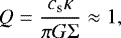 (22)
(22)
where κ is the epicyclic frequency. For smaller cooling parameters the disk fragments, which could stop the accretion process onto the central object. Therefore, we choose a few typical values for  in the vicinity of the critical value.
The cooling timescale depends on the local dynamical timescale (see Eq. (13), tdyn = 2πΩ = 2π × τdyn) and therefore is the range
![\begin{equation*} \tau_{\mathrm{cool}}\in b_{\mathrm{cool}}\times {[0.04,80]}~\textrm{Myr}. \end{equation*}](/articles/aa/full_html/2018/06/aa31688-17/aa31688-17-eq26.png) (23)
(23)
Thus, the weakest cooling of all simulations runs on a timescale of 800 Myr. In the case of the weakest cooling, we still reach two cooling timescales at the outer boundary until the simulation stops.
Furthermore, we define a power law for the temperature with a maximum near the inner boundary in simulations with an energy equation similar to the initial surface density distribution. The power law is given by
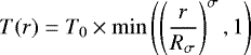 (24)
(24)
using σ = −1 and Rσ = 100 pc. The solutions are especially insensitive to the temperature especially in the inner region since there the cooling runs on very short timescales and an equilibrium state is reached very quickly. In addition, the simulation should start with a rather high temperatureso that the disk is Toomre stable, otherwise a unrealistic equilibrium state could be achieved as a direct consequence of the initialconditions.
Accretion disks usually present highly supersonic rotation, hence the kinetic energy dominates strongly over the internal energy. Despite the conservation of total energy, a consequent transfer of much internal to kinetic energy is possible, which means that the internal energy would become negative. To prevent this, we define a lower limit for the pressure so it has to remain positive. If the pressure falls below this limit, it is raised in these cells to its lower limit pmin
 (25)
(25)
The local pressure minimum is set by means of a global lower temperature limit Tmin, for example the cosmic microwave background temperature
 (26)
(26)
While analyzing the simulations the areas at a minimum temperature can be identified. This is usually only the case for very short time spans whenever highly dynamical events happen, for example a strong accretion event. Furthermore, rearward of the shocks small extremely cold regions can be generated that are reheated by their surroundings on short timescales.
3 Simulations with constant speed of sound
In this workwe focus on the impact of large-scale gas flows within a barred galaxy on the growth rate of its central black hole. The parameter space consisting of initial surface density and sound velocity is described in Table 2. The four values for the speed of sound can be associated with gas temperatures of T ∈{72, 652, 1811, 7244} K according to Eq. (19).
The generation of particular structures like nuclear rings and nuclear spirals are well described in Li et al. (2015); Seo & Kim (2013); Maciejewski (2004), and Piner et al. (1995).
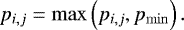
Nonetheless, we introduce the typical structure formation in our galaxy model by examining the isothermal simulation with an inital surface density of Σ0 = 10 M⊙ pc−2 and speed of sound of cs = 5 km s−1; in addition to the typical structures, this shows a quite laminar flow. Simulations with higher mass or lower speed of sound exhibit small spatially localized regions of significantly higher surface density than their surroundings. These clumps can modify or destroy the typical structures of the gas disk. Figures 2 and 3 show the surface density in these simulations at different zoom levels corresponding to radial scales R ∈{16 kpc, 6 kpc, 2 kpc, 300 pc}. In Fig. 2 (top) the bar potential is still raising. The surface density shows spiral structures on the kiloparsec scale that slowly bend. These spiral structures are a source of potential vorticity (Kim et al. 2012b) and can be subject to the wiggle instability (Wada & Koda 2004; Kim et al. 2014a). However the spatial resolution in this part of the computational domain is too low to resolve the instability at its early stages. The performed simulations only show the instability at smaller radii, which are reached shortly before the gas flows from the spiral structures into the nuclear ring region.
In Fig. 2 (bottom) the bar potential has reached its full strength. Now the spiral structures incorporate a nuclear ring with semi-axes of 2.5 kpc and 2 kpc. The ring often decays into individual clumps, since the high surface density material gains high vorticity from the spiral arms. If self-gravitation is disregarded but high spatial resolution is used, we often find clumps, which are generated by the wiggle instability at the spiral structures and are then transported to the ring region. The spiral structure changes its shape from slightly curved to nearly straight with a small angle inclined to the x-axis after the ring is generated. These structures, often called off-axis shock (Kim et al. 2012b), connect the ring on a radius of ~ 1 kpc with the region beyond 4 kpc. The gas outside the nuclear ring typically follows strong eccentric orbits. If it encounters one of the two off-axis shocks, it loses most of its rotational energy and descends to a smaller orbit or can be directly dragged by other material onto the nuclear ring (see Kim et al. 2012b). Thus the ring is fed with new matter. Furthermore, on large scales as well as inside the nuclear ring spiral arms can beidentified inside the nuclear ring.
In Fig. 3 the surface density of the nuclear ring has increased so much that has become gravitationally unstable. Atthe same time its eccentricity has decreased. The whole structure is shaped elliptically if it rotates counterclockwise. Inside the nuclear ring another ring-like (or disk-like) structure is recognizable. This again has a bar-like region of low surface density and two spiral arms.
Numerous observations show nuclear rings (Comerón et al. 2010; Fathi et al. 2015; Koay et al. 2016; König et al. 2016), off-axis shocks (Martini et al. 2003a,b; Prieto et al. 2005; van de Ven & Fathi 2010), and inner spirals and bars (Erwin 2004). Their formation is reproduced by comparable numerical examinations done by Roberts et al. (1979), Athanassoula (1992), Piner et al. (1995), Maciejewski (2004), Kim et al. (2012b), and Li et al. (2015). A detailed comparison of emerging structures with observations is given in Sect. 3.4.
An overview of all the simulations with constant speed of sound can be achieved by examining the mass of the central black hole as a function of time (Fig. 4). Most of the simulations reach considerable black hole masses of up to 4 × 10⁸ M⊙. All the simulations show a switch-on phase while the bar potential is activated, and reach one of two different states at about 370 Myr:
-
Simulations with a high speed of sound and low disk mass accrete slowly (s10*, s30c10);
-
Simulations with a low speed of sound and high disk mass accrete quickly (s30c1–s30c5, s50c*).
Though the transition of simulations from slow to fast accretion modes is clearly possible, the launch of the strong accretion mode is favored by high disk masses and a low speed of sound, as shown by the Σ0 = 30 M⊙ pc−2 and cs = {1, 3, 5} km s−1 simulations (Fig. 4). At the end of simulations with strong accretion the black holes grow with an approximately constant accretion, as will be shown later.
Summary of the mean and maximum accretion rates, structure formations (gravitational instabilities, GI), and final black hole masses for isothermal simulations.
 |
Fig. 2 Surface density of the simulation with Σ0 = 10 M⊙ pc−2 and speed of sound cs = 5 km s−1 on different scales of the central region after a half revolution of the bar t = 93 Myr (top) and after one revolution of the bar t = 186 Myr (bottom). |
 |
Fig. 3 Surface density of the simulation with Σ0 = 10 M⊙ pc−2 and speed of sound cs = 5 km s−1 on different scales of the central region after two revolutions of the bar t = 372 Myr. |
3.1 Weak accretion
The simulation with the surface density parameter Σ0 = 10 M⊙ pc−2 and cs = 3 km s−1 is an excellent example of the weak accretion case. Figure 5 (top) shows the black hole growth and the accretion rate as a function of time. The accretion rate never exceeds 10−2 M⊙ yr−1 and the Eddington outflow is on the same order. The bulk of the accreted mass arises from a short accretion phase after approximately 300 Myr. At this time Fig. 5 (bottom) shows clump formation. At later times the flow is predominantly laminar and two nuclear rings can be identified. In particular, the low-mass gap at around 300 pc seems to prohibit further accretion since no matter can flow into the inner disk (r < 300 pc). Therefore, the inner disk remains stable and more accretion is suppressed.
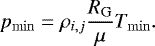
Figure 6 illustrates the time evolution of the simulation with higher initial mass (Σ0= 30 M⊙ pc−2) and greater speed of sound (cs = 10 km s−1). The mass of the nuclear ring at ~800 pc is sufficient to refill the inner disk after its initial mass loss. However, the relevant process here is not clumpy accretion, but loss of kinetic energy by shock compression (e.g., Shore 1992). Since this is an isothermal simulation, the gas temperature stays constant. In order to illustrate how the gas moves in the inner areas, Fig. 7 depicts the velocity field using instantaneous streamlines. When passing through a shock, a substantial fraction of the kinetic energy is dissipated leading to a decelaration along the azimuthal direction. Hence, gravitational forces are no longer balanced by centrifugal forces and therefore the gas experiences a net radial force which causes a radial inflow. It should be noted that the dissipated energy is lost because the temperature is kept constant in the isothermal simulations. The accretion rate onto the black hole (Fig. 6) is in the range 10−3⋯−2 M⊙ yr−1 without large deviations for more than 90% of the time.
It should be noted that the accretion rate and Eddington outflow rate are mean values taken over the period between two data outputs and can therefore not resolve fluctuations, which are shorter than Δt = 1.86 Myr. If the accretion rate exceeds the Eddington limit even for a short period <1.86 Myr, outflow is generated, although the mean accretion rate never reaches the Eddington limit (see Fig. 6). Thus, in this simulation less than ~ 5 × 10⁵ M⊙ is lost by means of the Eddington limit because the accretion rate is almost constant and the Eddington outflow rate is usually below 10−4 M⊙ yr−1. Shortly before the end of the simulation, the inner disk reaches a mass of about 108 M⊙, which is the requirement for strong accretion, as is discussed in the next section.
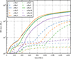 |
Fig. 4 Evolution of the black hole masses of all different parameter combinations in the isothermal simulations. We note that there are two very different accretion modes. The simulations with Σ0 = 30 M⊙ pc−2 show that the lower the speed of sound, the earlier the simulation switches to the strong accretion mode and the higher the final black hole mass is. |
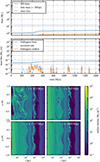 |
Fig. 5 Time evolution of the simulation with Σ0 = 10 M⊙ pc−2 and speed of sound cs = 3 km s−1, as an example of weak accretion. Top: after the bar is switched on the accretion rate rises for a short period. Afterward it declines and falls below 10−4 M⊙ yr−1. Bottom: at the beginning of the simulation the surface density shows fragmentation in the inner region. Later the flow in the inner disk is laminar. Eccentric nuclear rings can be identified at 80 pc and 800 pc. |
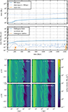 |
Fig. 6 Time evolution of the simulation with Σ0 = 30 M⊙ pc−2 and speed of sound cs = 10 km s−1, as an example of weak accretion with central shocks. Top: simulation showing a steady accretion rate of 10−3⋯−2 M⊙ yr−1. Bottom: firstfragmentation occurring around 100 pc and inside the nuclear ring at 800 pc. Later onthe inner fragmentation fades and a rather eccentric ring and inner shocks form at 80 pc. |
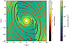 |
Fig. 7 Instantaneous streamlines and surface density map of the simulation with Σ0 = 30 M⊙ pc−2 and speed of sound cs = 10 km s−1. At the shocks the gas is compressed and loses a great part of its kinetic energy. Its velocity becomes subsonic and the gas is pushed to lower radii until it again reaches sufficient velocity to balance centrifugal and gravitational forces. This process can drive the gas far into the inner disk within a few orbits. |
3.2 Strong accretion
First we consider simulations, where the strong accretion starts at a later point in time after the switch-on process is finished. Figure 8 (top) shows the time evolution of accretion rate, Eddington outflow rate, and black hole mass for the simulation with Σ0 = 30 M⊙ pc−2, cs = 3 km s−1. During the initial phase of about 800 Myr, the accretion rate and the outflow rate are roughly on the same order and decrease from 10−2 M⊙ pc−2 to below 10−4 M⊙ pc−2. In this phase we observe strong variations which indicate clumpy accretion. From time to time individual clumps cross the inner boundary leading to accretion rates above the Eddington limit for short periods. This does not show up in the diagram because the outlined accretion rate sums the accretion between two data outputs over a period of 1.86 Myr. Therefore, short-lived accretion events cannot be resolved. Figure 8 (bottom) shows the surface density for four selected points in time. The figure for 372 Myr supports the observation of a clumpy accretion, given that multiple clumps are visible in the inner disk. The free-fall timescale of a clump at radius R = 30 pc for the initial black hole mass M = 106 M⊙ is τff = 2.45 Myr. This is comparable to the time resolution of the simulations for data outputs of 1.86 Myr. Thus, it cannot be expected to directly observe the infall of a clump.
This first clumpy accretion phase is completed after 745 Myr since the flow has adapted to the fully switched on bar potential and there is no further accretion. In the inner disk we find three round rings (Fig. 8, bottom, vertical lines in this projection). Initially the mass of the inner disk (< 300 pc) is reduced by approximately 5 × 10⁶ M⊙. Starting at the region around 1 kpc the accretion disk becomes gravitationally unstable (Safronov 1960; Toomre 1964; Paczynski 1978; Kozlowski et al. 1979; Rafikov 2015), which drives an accretion flow inward. Therefore the inner regions start gaining mass and the unstable region expands inward. At 400 Myr the inner disk mass (r < 300 pc) starts increasing. If the mass in the inner disk reaches 108 M⊙, it becomes gravitationally unstable and the strong accretion mode, which is initially very clumpy, sets in. This kind of gravitational instability, which generates individual gravitationally bound structures, is typical for systems on very short cooling timescales (Gammie 2001). In this case an isothermal equation of state is used, which is equivalent to an instantaneous cooling, since the gas cannot be heated by compression. The Toomre parameter (Toomre 1964) characterizes whether gravitational instabilities can be expected in an accretion disk. The parameter is proportional to  . Since the temperature is constant in this case, a stable state Q > 1 can only be reached again by decreasing the surface density Σ. If the accretion disk becomes Toomre unstable by accumulation of mass, gravitational instabilities arise.
Figure 8 (bottom) already shows the generation of instabilities at a radius of 800 pc at 372 Myr, which spread until 1117 Myr to smaller and smaller radii, and therefore lead to an increase in the inner disk mass. After about 1100 Myr the accretion rate settles at 10−1 M⊙ yr−1 and the outflow rate declines. From this time on the inner disk mass stays approximately constant at 1.5 × 10⁸ M⊙. The inner disk is supplied with mass from the outer disk at the same rate as mass flows over the inner boundary, which is then accreted by the black hole. The Eddington outflow is about one order of magnitude below the accretion rate at the end of the simulation. An examination of the surface density distribution reveals that the accretion is less clumpy than before. Instead, clumps are so numerous in the central disk < 10 pc that they are sheared out to density filaments. The accretion flow is still equally strong, but smoother and less abrupt, and there are three different epochs:
-
0–800 Myr, where an initial accretion flow of 10−4…−2 M⊙ yr−1 sources its matter from the inner disk and refills it from outside;
-
800–1100 Myr, where the inner disk is still being filled and drives a strong clumpy accretion flow 10−2…−1 M⊙ yr−1;
-
1100–1600 Myr, where strong accretion with a constant rate of 10−1 M⊙ yr−1 takes place and the inner disk is refilled from outside at the same rate.
The simulation with initial surface surface density Σ0 = 50 M⊙ pc−2 and speed ofsound cs = 3 km s−1 is the isothermal simulation with the highest black hole mass at the end of the simulation time. The simulation experiences a switch-on phase, which directly leads into a strong accretion mode since an inner disk mass of > 108 M⊙ is already reached after 300 Myr. Figure 9 shows an initially clumpy accretion with strong Eddington outflow. Afterward, up to a radius of about 100 pc, mainly filamentary structures can mainly be identified. At 1000 Myr the accretion rate settles down to 2 × 10⁻¹ M⊙ yr−1, and the Eddington outflow decreases. In addition, the unstable region between 100 pc and 1 kpc no longer shows clumps; instead, this region is dominated by a filamentary flow.
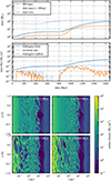 |
Fig. 8 Time evolution of the simulation with Σ0 = 30 M⊙ pc−2 and speed of sound cs = 3 km s−1, as an example of strong accretion. Top: after a half revolution of the bar, a strong clumpy accretion flow with high Eddington outflow already starts, and decreases with time. Later on the strong accretion is established, which again is highly clumpy at first and reaches an accretion rate of 0.1 M⊙ yr−1. Bottom: initial clump formation is observed in the inner disk, but fades quickly. Then the inner disk becomes laminar until the strong accretion sets in. Afterward, the complete disk inside 1 kpc exhibits strong clump formation before a gravitational turbulent mode is reached. |
3.3 Time evolution of black hole masses
Figure 4 shows that cold disks with higher initial mass (e.g., cs = 3 km s−1 and Σ0 = [50]M⊙ yr−1) induce faster accretion, which then leads to higher black hole masses at the end of the simulations. Table 2 outlines the mean accretion rates and the final black hole masses. Again, this indicates that massive gas disks accrete more strongly. For simulations with Σ0 = 10 M⊙ pc−2 the maximum accretion rate is 0.02 M⊙ yr−1 and the temporal mean is even below <10−2 M⊙ yr−1. Nuclear rings can only persist in the least massive simulations, and even here they are clumpy because of the high surface densities. In the massive simulations the rings are so dense that they fragment and their structures disintegrate. Furthermore, if strong accretion sets in very early, ring formation can be suppressed completely. This
may only happen in simulations with the highest initial mass. The inner disk exhibits mostly gravitational instabilities (GI) for the isothermal simulations. Only the mass-poor simulations with high sound velocities show the formation of tightly wound inner spiralsor strong shocks. Clearly this is a more efficient accretion mechanism than in the simulations with Σ0 = 10 M⊙ pc−2.
A variation in the sound velocities tends to result in varying final black hole masses, but more importantly influences if and when the strong accretion starts. Figure 10 shows the accretion rates of all isothermal simulations. The different accretion types are clearly distinguishable. The accretion rate is either greater than 0.1 M⊙ yr−1 or below 0.01 M⊙ yr−1. It is striking that all the simulations show strong variability in the accretion rate. This is probably because the inner boundary of the computational domain at 2 pc is not close enough to the black hole, and therefore an important part of the accretion disk lies outside the computational domain. It is still assumed that the mass that leaves the computational domain across the inner boundary is directly accreted onto the black hole. This is especially problematic for clumpy accretion. At small radii the differential rotation becomes stronger and stronger, hence the clumps would be sheared out to density filaments. The accretion of filaments is much more continuous, so that the effective accretion rate onto the black hole might be closer to the Eddington limit.
A special case is the simulation with Σ0 = 10 M⊙ pc−2 and a speed of sound of cs = 10 km s−1. Here from [800] Myr onward the accretion rate oscillates with a period of about 20–25 Myr (Fig. 10, red line). On closer examination of the density structure at different times, the origin of the periodicity becomes clear. In this simulation a nuclear ring develops and, since the onset of the periodicity, an inner shock becomes visible. The eccentric nuclear ring oscillates on the above-mentioned time scales, and therefore ejects mass at regular intervals across shocks into the inner disk region and the black hole. The oscillation period decreases slowly with time. The oscillation does not fade; instead, it remains stable for more than 800 Myr.
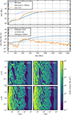 |
Fig. 9 Time evolution of the simulation with Σ0 = 50 M⊙ pc−2 and speed of sound cs = 3 km s−1, as an example of strong accretion. Top: simulation reaching the highest final black hole mass of all the simulations carried out for this work. During the switch-on phase an inner disk mass of more than 108 M⊙ is reached. This leads immediately to strong accretion of more than 0.1 M⊙ yr−1 right from the beginning. Bottom: simulation initially exhibiting strong fragmentation, before changing to a gravitational turbulent accretion mode. A laminar inner disk is never observed. |
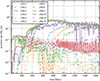 |
Fig. 10 Plot of the accretion rates of all isothermal simulations. It is clearly visible that the simulations all lead either to strong accretion of more than 0.1 M⊙ yr−1 or to weak accretion of less than 0.01 M⊙ yr−1. Additionally, all simulations exhibit strong variations in the accretion rate. |
3.4 Discussion
Clumpy accretion plays an important role in many of the examined simulations. Primarily isothermal simulations with strong accretion encounter Eddington outflows that are almost as strong as the accretion rate. The simple implementation of the Eddington limit may not be sufficient any longer. On the one hand, a substantial part of the accretion disk is outside the computational domain at radii < 2 pc. Here clumps could decay to a more homogeneous disk, which transports the matter more continuously to the black hole. Also, new clumps could not be formed in the innermost part of the disk since it is not self-gravitating and therefore Toomre stable. This would be especially important for the infall of single massive clumps. However, if the outflow rate is uniformly very high, there would be no particular effect. On the other hand, the Eddington limit is not a strict maximum of a variable accretion rate. It describes the equilibrium state of the balance of gravitational forces and Thomson scattering (Rybicki & Lightman 1979; Frank et al. 2002). This means that massive clumps with strong inward directed momentum, which can be observed after a typical clump-clump interaction for example, are slowed down by the Thomson scattering, but still reach the black hole. However, in order to model these effects we have to resolve the flow within the inner disk on the subparsec scale. These model limitations require the interpretation of the measured accretion rates as lower limits especially in the case of clumpy accretion. The accretion rate and Eddington outflow of such a simulation are shown in Fig. 9 (top). Nonetheless, the total effect on the final black hole mass can be neglected; even if the Eddington limit were not applied, the black hole would gain at most a factor of 2 in mass. However, an overall different evolution of the simulation and accretion would be conceivable since the mass loss by means of the Eddington limit has an influence on the mass and therefore on the relevance of self-gravitation in the inner disk.
Nuclear rings are observed in a multitude of systems (Martini et al. 2003a,b; Fathi et al. 2015; König et al. 2016; Koay et al. 2016), some with clearly clumpy structures (e.g., Xu et al. 2015) and even in the galactic center (Lau et al. 2013). The observations feature surface densities of 102 M⊙ pc−2 (Fathi et al. 2015) in the inner kiloparsec and up to 104 M⊙ pc−2 for the clumpy rings (Xu et al. 2015). However the measurements are subject to large uncertainties, especially because of the required conversion factor from the indicator HCN to the gas density. The clumpy ring structures are consistent with the results in this work, which show in the area around 100 pc densities of up to 104 M⊙ pc−2.
Fathi et al. (2015) have determined a stability parameter Q (Romeo & Wiegert 2011; Romeo & Falstad 2013) similar to the Toomre parameter for their HCN gas observation, which takes the disk thickness into consideration. They conclude that the inner disk <500 pc is stable and the ring region ~800 pc is unstable. The simulations in this work often exhibit a gravitationally unstable inner disk (< 300 pc) for the region inside of a nuclear ring (<300 pc). This cannot be confirmed by the observations, and is evidence that stabilizing elements should be considered. Possibly, an effective speed of sound that includes the stabilizing effects of small-scale turbulence should be leveraged (Romeo et al. 2010).
4 Simulations with cooling
The results from the simulations with cooling are considerably more complex than the results from the isothermal simulations. Several different solutions for the surface density and temperature structure exist, which affect the accretion onto the black hole significantly.The examined parameter space consists of the initial surface density and the dimensionless cooling parameter, and is shown in Table 3.
First, we look at the black hole masses of all simulations as a function of time in Fig. 11. A few simulations start directly accreting as a consequence of the initial conditions. After about one rotation of the bar all simulations accrete near the Eddington limit. The trigger seems to affect the simulations that accrete below this limit, which now also accrete at the Eddington limit.
Figure 12 exposes the common trigger of this very strong accretion mechanism. Similarly to the isothermal simulations, the bar potential induces strong shocks in the gas, which grow in curvature with time. In this case, however, the shocks do not connect to form a ring or clumpy ring, but bend further and migrate inward untilthey touch the inner boundary of the computational domain. Here they stay fixed, while the outer parts spread matter in chaotic shocks in all directions. In the process the spiral arms heat the inner disk to very high temperatures (106 K). The shocks are a very effective mechanism for transporting the gas to the galaxy center (Athanassoula 1992). Figure 13 shows that the gas dissipates a great deal of its kinetic energy at the shocks, therefore heats its surroundings, and closes in on the black hole because of its low rotational velocity. Thus, the orbits become extremely eccentric even in the direct vicinity of the black hole, whose gravity is already very important. The black hole growth shows that this enables a very effective accretion flow.
The accretion at the Eddington limit cannot be sustained after a short time by the Σ0 = 10 M⊙ pc−2 simulations. Subsequently, all of them accrete more slowly until those with strong cooling abruptly diminish their accretion rates and accrete more weakly (tcool ∈{1, 3} after 350 Myr and 500 Myr, respectively). We considerthis cold accretion mode in more detail in the following section.
Summary of the mean and maximum accretion rates, structure formations (gravitational instabilities, GI), and final black hole masses for simulations with cooling.
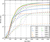 |
Fig. 11 Summary of the black hole growth for the complete parameter study of the galaxy simulations with cooling. All the simulations accrete at the Eddington limit; the accretion then decreases heavily for simulations with strong cooling. |
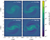 |
Fig. 12 Shock generation in simulations with energy equation similar to the isothermal simulations with Σ0 = 30 M⊙ pc−2 and bcool = 1. The shocks do not connect to a ring, but bend further until they touch the inner boundary of the computational domain. |
4.1 Cold accretion
An example of cold accretion is the simulation with Σ0 = 10 M⊙ pc−2 and cooling parameter bcool = 1. Figure 14 shows the accretion rate and the Eddington mass loss as a function of time. After the strong accretion phase, which all the simulations experience initially, the accretion rate weakens in this simulation past 370 Myr very quickly. At the time when the accretion rate has completely collapsed, a steady accretion flow of initially 4 × 10⁻³ M⊙ yr−1 starts, which decreases exponentially with time. A mass loss by means of the Eddington limit as has been observed for strong accretion does not occur. Even so, within a short period more than 107 M⊙ is lost, which is approximately the same amount the black hole has accreted. The most important feature of this plot is the drop in accretion rate shortly afterthe mass of the inner disk starts decreasing. Prior to this a fast growth phase takes place, which is completed after about 300 Myr. This is probably a switch-on effect, whichstarts at t = 186 Myr when the bar has reached its full strength. There are no indications that this process might be repeated at a later time. The inner disk loses more mass than is accreted by the black hole or than is removed by the Eddington limit from the system. Therefore, the inner disk transfers mass to the outer regions of the galaxy.
Figure 15 shows the surface density structure during the strong accretion and after the drop in accretion rate. In the strong accretion phase the flow in the kiloparsec region is comparatively chaotic. Ring-like structures are indeed present, but they are quite amorphous, and a large amount of gas flows along the bar onto these central structures.
At the time when the accretion rate shows a considerable decline, a marginally stable self-gravitating disk forms in the center. This means that gravitational instabilities arise if an accretion disk becomes Toomre unstable by cooling or accumulation of mass. These instabilities dissipate energy and heat the accretion disk. Since the cooling is weaker than the heating by the instabilities, the Toomre parameter increases to Q > 1 and the disk becomes stable again.Given that the cooling still operates, this process will start over again. Therefore, a marginally stable state is reached with a Toomre parameter of Q ~ 1, as has been predicted by Paczynski (1978). This can be achieved in non-isothermal systems with slow cooling (Paczynski 1978; Rice et al. 2003, 2005; Durisen et al. 2007; Cossins et al. 2009, 2010). Therefore further accretion would be expected as a result of the marginally stable accretion disk.
Given that the region outside the accretion disk is very gas poor, no effective coupling with the disk can be established. Angular momentum cannot be transported from the accretion disk to outside regions (see Illenseer & Duschl 2015).
Withoutangular momentum transport, there can be no accretion. Therefore, such gas-poor regions are of great importance. Figure 16 shows the time evolution of the azimuthally averaged density profiles of all isothermal and non-isothermal simulations. Gas-poor regions of different strengths can clearly be seen in all simulations. The outer boundaries of these regions coincide roughly during almost the whole simulation with the position of an inner Lindblad resonance. Therefore, slightly disturbed gas loses its orbit and is pushed inward. High angular momentum material coming from smaller radii cannot cross this boundary to transport angular momentum outward (Hopkins & Quataert 2010).
The developments of the other simulations in Fig. 11 show that most of them accrete close to the Eddington limit for a much longer time. Also, both simulations with Σ0 = 10 M⊙ pc−2 and weak cooling accrete more mass than the simulations with strong cooling. This case of hot accretion is discussed in the following section.
 |
Fig. 13 Strong shocks along the bar which strongly heat the gas. The loss of kinetic energy results in a decrease in the orbits of fluid particles, which quickly reach the central disk on spiral paths. |
 |
Fig. 14 Time evolution of the accretion rate, the Eddington outflow, and the black hole mass of the simulation with Σ0 = 10 M⊙ pc−2 and bcool = 1. Disregarding of a short accretion phase after the bar is switched on, there is only weak accretion. |
 |
Fig. 15 Surface density of the simulation with Σ0 = 10 M⊙ pc−2 and bcool = 1 at different spatial scales. Top (253 Myr): in the center an irregular ring can be seen. The overall structure is very chaotic and some high-mass fragments are perceivable. Bottom (744 Myr): in the central region a marginally stable self-gravitating disk has formed, embedded in a gas-poor environment. Thus, the central accretion disk couples only weakly to the kiloparsec-scale gas disk. Angular momentum transfer to the outer parts of the galaxy is suppressed and consequently the accretion rate onto the black hole declines. |
4.2 Hot accretion
A typical case of the strong accretion and weak cooling is represented by the simulation with a surface density of Σ0 = 30 M⊙ pc−2 and the cooling parameter tcool = 6. Figure 17 shows the accretion rate and the Eddington outflow as a function of time. Even before the bar potential is completely switched on, substantial accretion onto the central object takes place. Up to 600 Myr the accretion rate is close to the Eddington limit, while the outflow rate indicates an occasionally clumpy accretion. The accretion rate reaches its maximum value of 2 M⊙ yr−1 after 600 Myr. It then declines exponentially at a rate of 3 Gyr until it settles down at a constant rate of 0.1 M⊙ yr−1 for the remaining 200 Myr of the simulation. The course of the accretion rate seems to be closely correlated to the mass of the inner disk, for example the maximum inner disk mass of 3 × 10⁸ M⊙ is reached shortly before the maximum accretion rate. The inner disk passes the matter coming from outside to the inner region with some delay. The inner transport mechanism conforms with the previously described energy dissipation at strong shocks (Sect. 4), as illustrated in Fig. 13. At the start of every simulation there are two shocks in the central region that dissipate kinetic energy and therefore generate a hot inner region with the gas spiraling in and approaching the center on eccentric orbits. Thus, angular momentum can quickly be transported outward and mass can efficiently be accreted.
The hotaccretion mode can also be distinguished from the cold accretion mode by the time evolution of the azimuthally averaged density profile (see Fig. 16). The simulations that show the hot accretion mode have a high-density inner disk <20 pc with a sharp outer boundary to larger radii. Additionally, the low-density region beyond 1 kpc is less pronounced as a result of the accretion flow from the kiloparsec scale.
 |
Fig. 16 Time evolution of the azimuthally averaged surface density profile of all the simulations performed. |
 |
Fig. 17 Time evolution of the accretion rate, Eddington outflow, and black hole mass of the simulation with Σ0 = 30 M⊙ pc−2 and bcool = 6. Even before the bar potential is switched on completely (186 Myr), there is strong clumpy accretion. The inner disk mass rises quickly and high accretion rates up to 2 M⊙ yr −1 are attained. Later on the Eddington outflow declines much more quickly than the accretion rate. This suggests a decrease in the clumpy accretion. |
4.3 Time evolution of black hole masses
All simulations with cooling lead to the hot or cold accretion mode. Which of the two is achieved does not depend on the initial mass, but instead on the cooling parameter. Figure 11 shows an example of a mass-poor simulation with Σ0 = 30 M⊙ pc−2 where the exact cooling parameter is not important in the chosen parameter space, but only if it is below or above a specific critical value.
The final black hole mass depends on the initial disk mass and the accretion mode. The resulting black hole masses of the cold and hot accretion modes differ in these simulations by around a factor of five. The dependence of the final black hole mass on the initial disk mass does not change significantly between isothermal and non-isothermal simulations, as shown by the simulations with bcool = 3 in Fig. 11.
The massive disk simulation with Σ0 = 50 M⊙ pc−2 and bcool = 3, however, seems to be an exceptional case. It leads to an intermediate value for the final mass, about a factor of two more massive than in the simulation with bcool = 1, but less massive than in the other simulations with the same initial disk mass. The accretion mode seems to be somewhere in between the cold and hot modes. The threshold of the cooling parameter seems to be weakly dependent on the disk mass. In this case the transition region between the two modes has been exactly met.
Figure 18 shows the accretion rates of all galaxy simulations with cooling. In contrast to the isothermal simulations there is no clear trend that allows us to distinguish between strong and weak accretion accretion. The simulations with Σ0 = 10 M⊙ pc−2 show an accretion rate of less than 5 × 10⁻³ M⊙ yr−1 at the end of the simulation period. Simulations, however, with higher initial surface densities exhibit peak accretion rates of more than 2 × 10⁻² M⊙ yr−1 before their accretion rates start to decline exponentially at about 800 Myr.
Table 3 lists the mean and maximum accretion rates, as well as the final black hole masses. Hot simulations with weak cooling and Σ0 = 30 M⊙ pc−2 reach higher black hole masses than the massive simulations with cold accretion. All simulations with bcool = 10 reach the highest black hole masses and accretion rates. Table 3 also shows which structures in the inner disk form, and weather or not nuclear rings arise and persist for a long time. This happens only for the least massive disks; otherwise, gravitational instabilities set in which prohibit their formation at all or lead to their disintegration rather quickly. In the case of strong cooling, the inner disk becomes gravitationally unstable and any large-scale structures that are generated initially in all simulations are destroyed immediately due to fragmentation. Only in the hot simulations with weak cooling do these shocks persist throughout the whole simulation and do not become unstable in the inner regions.
Figure 19 reveals the radial azimuthally averaged temperature of the simulation with Σ0 = 30 M⊙ pc−2 for several cooling parameters. The temperatures in the simulations with cooling match those with cold accretion up to radii of 1 kpc to the warm ionized medium (Gnedin et al. 2015). This matches also within the area below about 10 pc in the case of simulations with hot accretion. Beyond a 10 pc radius the simulations with hot accretion reach temperatures as high as 105 –106 K, which corresponds to the typical temperatures of hot ionized gas (Ferrière 2001). The temperatures in the isothermal simulations agree with molecular gas ~100 K and the warm neutral or ionized medium (Ferrière 2001).
 |
Fig. 18 Accretion rates of all galaxy simulations with cooling. The simulations with Σ0 = 10 M⊙ pc−2 initial surface density show considerably lower accretion rates than the others at the end of the simulations. The massive simulations feature exponential decreasing accretion rates of low variation from 800 Myr onward. |
 |
Fig. 19 Azimuthally averaged temperature curve of the non-isothermal simulations with Σ0 = 30 M⊙ pc−2. In the area <1 kpc, the simulations with strong cooling show temperatures that can typically be found in the warm ionized medium. In contrast, the simulations with weak cooling feature very high temperatures up to 106 K. |
4.4 Discussion
So far the involved temperatures in the simulations have not been discussed in detail because the cool function is independent of the temperature. The temperature only goes indirectly into the simulations by means of the gas pressure and the speed of sound, and thereby intothe Toomre criterion, even though the speed of sound is a very important temperature dependent quantity that plays an important role in every hydrodynamic simulation. All simulations with cooling initially encounter a strong shock that heats the gas inside 1 kpc to very high temperatures of 105…6 K. These temperatures can still be observed at the end in simulations with weak cooling. Although very high temperatures up to ~ 6 × 10⁵ K can be obtained in the vicinity of the black hole (Alexander & Hickox 2012) it should be questioned whether this extends to the whole central region of a galaxy. Additionally, it should be noted that hot ionized gas is generated by shock compression due to supernova explosions (McKee & Ostriker 1977). These events produce extended hot bubbles of low density in the interstellar medium (Scannapieco et al. 2008; Seitenzahl et al. 2013; Krause et al. 2014). These might reach temperatures that are comparable to our simulation; however, they are spatially and temporally very confined. Therefore, their impact on the azimuthally averaged temperature will be small.
Overall, the processes that contribute to the cooling and heating of the gas have to be modeled in greater detail. In this work only the contribution of shock and compression heating and a simple cooling in dependence on the dynamical timescale are considered. The selection of the cooling parameter in our simulations is motivated by the the critical value bcool (Gammie 2001), which is known to produce a gravitationally turbulent flow. The actual cooling processes run on timescales of ~ 10−6⋯−4τdyn (Hopkins & Quataert 2010). Also, the heating by supernova explosions operates on timescales much shorter than the dynamical timescale (see Sect. 2.3). Thus, the cooling employed in this work should model the effective contribution of the balance of all actual cooling and heating processes. The leveraged hydrodynamics software FOSITE (Illenseer & Duschl 2009) provides the opportunity of cooling using the method from Hubeny (1990), which models a gray radiation with mean Rosseland opacities according to Bell & Lin (1994). The key issue is that the complete gas is immediately cooled down to the minimum allowed temperature (see Sect. 2.3). This is inevitable because no explicit heating has been included, since a model of the heating processes is extremely difficult. The interstellar medium is predominantly heated by bright young stellar clusters and supernovae (Kravtsov & Yepes 2000). Supernovae can be heated extremely well by means of shock compression and momentum input and are especially important for the inner galaxy disk areas of high density, which exhibit high opacities and star formation (e.g., Seo & Kim 2013; Kim & Ostriker 2015), although these are processes that cannot be resolved in the simulations carried out in the present work. Therefore, modeling the heating processes appropriately requires a subgrid-scale model that accounts for star formation (radiation input) and supernova feedback. The result is gas turbulence on smaller scales than the mesh of the hydrodynamic simulations. In order to model these movements on the smallest scales, turbulent pressure can be introduced (Murray et al. 2010; Alexander & Hickox 2012), which together with the thermal pressure results in effective pressure (Springel & Hernquist 2005; Springel et al. 2005; Robertson et al. 2006). This effective pressure is sufficient to prevent collapse on small scales, and increases the Toomre parameter and the Jeans length. For example, Murray et al. (2010) use turbulent sound velocities on the order of 10–100 km s−1, which are consistent with observations (e.g., Downes & Solomon 1998). The high sound velocities found in the simulations in this work can therefore be interpreted as effective sound velocities, which are composed of thermal and turbulent pressure and which motivated Kim et al. (2012b) to use high isothermal sound velocities of up to 20 km s−1.
If we consider the high temperatures obtained in the simulations to be realistic values, this would imply the existence of ionized gas. Hence, magnetic fields could play an important role in hydrodynamics. Kim & Stone (2012) performed two-dimensional non-self-gravitating magnetohydrodynamic simulations of barred galaxies. They report that all simulations show nuclear rings and that the typical spiral arms have lower densities than in hydrodynamic simulations. Also, initially there is a second bar (Shlosman et al. 1989) inside the nuclear ring in accordance with observations (e.g., Shaw et al. 1995; Friedli et al. 1996). Furthermore, Kim & Stone (2012), report mean accretion rates of about 10−4…−2 M⊙ yr−1. Since they do not account for self-gravity of the gas disk nor do they consider the influence of an outer spiral structure on the potential, they do not obtain a persistent mass flow from the outer regions onto the central disk after a short initial accretion phase.
5 Impacton AGN evolution
The gathered black hole masses and accretion rates can be combined to evolutionary tracks of the different black holes in an AGN luminosity-mass-diagram (cf. Shen et al. 2008; Steinhardt & Elvis 2010). If we assume a black hole accretion efficiency (Davis & Laor 2011) of η= 0.1, the AGN luminosity can be calculated as a function of the accretion rate Ṁ
 (27)
(27)
Figure 20 shows that only simulations with Σ0 = 30 M⊙ pc−2 or Σ0 = 50 M⊙ pc−2 result in noteworthy evolutionary tracks. The mass-poor simulations nearly vanish in this diagram because only very low black hole masses could be reached. The other simulations proceed partially along the Eddington boundary, but half a decade below because of the above-mentioned effect of clumpy accretion and because the inner boundary of the computational domain is at a comparatively large radius. A disproportionately high amount of mass is lost by means of Eddington outflow. All the massive simulations eventually deviate from the track along the Eddington boundary. In the beginning they accrete more slowly and later decrease further. Unfortunately, the simulation time is not long enough to follow until the accretion is finished and the accretion rate collapses completely.
In contrast to the isothermal case the simulations with cooling show considerable black hole growth. Thus, Fig. 21 of the AGN luminosity–mass plot shows long evolutionary tracks for all simulations with cooling. The evolutionary tracks all look very similar: First, an accretion phase near the Eddington limit takes place, whichcan be strongly fluctuating. This could be caused by the remaining distance of the black hole to the inner boundary of the computational domain, as has been explained in detail in Sect. 3.3. After some time, depending on the parameters, the simulations stop accreting at the Eddington limit and bend down to gradually weaker AGN luminosities. Often the decline is very abrupt so that the black hole only grows marginally.
Steinhardt & Elvis (2010) plot the luminosities of more than 60 000 quasars against their black hole masses depending on their redshift. They observe that quasars with low black hole masses of up to 107 M⊙ can reach luminosities as high as their respective Eddington luminosities, but higher mass quasars are subject to a second boundary below the Eddington luminosity (cf. Kollmeier et al. 2006; Caplar et al. 2015; Steinhardt & Speagle 2014). The observed ensemble is bounded from below by the detection limit at 1045 erg s−1. Unfortunately, this limits the comparability to the isothermal simulations. Here only the most massive simulations reach luminosities of more than 1045 erg s−1 since the maximum AGN luminosity, which is achieved for an accretion rate at the Eddington limit, is proportional to the black hole mass. Therefore, additional simulations reaching higher black hole masses would be desirable. In agreement with the observations the simulations are below the sub-Eddington limit, but without a larger sample of simulations we cannot give statistically relevant evidence.
The youngest quasars, which reach black hole masses comparable to those in our non-isothermal simulations (up to 2 × 10⁹ M⊙), have a redshift of z ≈ 0.8. We plot in Fig. 21 the sub-Eddington limit from Steinhardt & Elvis (2010) for quasars with a redshift of 0.6 < z < 0.8 (black dashed line). The results of the simulations comply with this limit very well before their accretion rates quickly decline. The argument would become stronger if simulations with higher initial disk masses were available.
 |
Fig. 20 Evolutionary tracks of the black holes in the isothermal simulations. Since only the massive simulations lead to appreciable black hole masses, the mass-poor simulations remain in the lower left corner. The other simulations move on a path parallel to the Eddington limit (black line), then they bend and feature a constant accretion rate. The dashed black line indicates the sub-Eddington limit for redshifts of 0.6 < z < 0.8 from Steinhardt & Elvis (2010). It does not pose a strong limit for these simulations. |
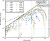 |
Fig. 21 Evolutionary tracks for the black holes of galaxy simulations with cooling. All simulations accrete for a long time near the Eddington limit (black line). Depending on the initial conditions they leave this evolutionary path at different black hole masses and then show strongly declining AGN luminosities. The dashed black line indicates the sub-Eddington limit for redshifts of 0.6 < z < 0.8 from Steinhardt & Elvis (2010). |
6 Conclusions
In this work we have analyzed isothermal and non-isothermal multi-scale simulations of the gas flow in barred spiral galaxies with particular attention to the growth of the central black hole. In the case of isothermal disks we could show that the simulations evolve in two completely distinct ways depending on the speed of sound and the initial mass of the gas disk. In the strong accretion mode the inner accretion disk (r < 300 pc) gains more than 108 M⊙, which causes the inner disk to become gravitationally unstable, thus leading to very efficient accretion.
In the weak accretion mode, however, the mass M of the inner disk is too low to drive a graviturbulent accretion. Instead, kinetic energy is dissipated at large-scale shock fronts, which leads to gas flow on eccentric and inward spiraling orbits, driving a weak accretion flow. In agreement with observations, nuclear rings and spirals can be observed at least for transitory periods in the simulations. Often these regular structures are destroyed because the inner disk gains mass and becomes gravitationally unstable.
In the second part of this paper we extended the models by accounting for energy transport, shock heating, and radiative cooling. Again, we were able to identify two modes of accretion in the simulations that are, however, completely different from the isothermal case. In the cold accretion mode the accretion rate is generally lower. Since a sufficient cooling is given, a marginally stable accretion disk is formed, but the accretion is mostly depleted after a short time because no further material is supplied from the kiloparsec region.
For the hot accretion mode, two remarkable shocks reach from the inner rim of the simulation domain up to the kiloparsec region. At these shocks energy is dissipated and the gas spirals inward on highly eccentric orbits. This is a very efficient accretion mechanism with typical accretion rates of 10−1…0 M⊙. The assigned AGN evolutions are in very good agreement to the sub-Eddington limit, but a physical explanation for this phenomenon remains hidden and requires the exploration of a larger parameter space.
Of course our models show some opportunities for improvement. The fixed gravitational potential of the stellar component might change over the course of such long-running simulations. The energy budget in the non-isothermal simulations is based on a very simple cooling model, which lacks the inclusion of various feedback mechanisms. Also, if the disk becomes hot, the vertical pressure scale-height will increase. In this case the approximation as a geometrical thin disk has to be dropped.
In comparison to Kim et al. (2012b) our results show the importance of self-gravity for the dynamical evolution of the gas disk. While they did not report overall significant black hole accretion, we were able to follow the evolution of the black hole for much longer(nine bar rotations) and found sustained high accretion rates. In many simulations graviturbulent accretion modes or filamentary structures were observed in the inner accretion disk. For this reason it is important to resolve the central accretion disk until the gravitational potential of the black hole dominates and the orbits become round with Keplerian velocities. Kim et al. (2012b) have also measured gas inflow for several simulations, but they note that simulations with black hole masses below 108 M⊙ suffer from non-circular orbits near the inner boundary of the computational domain, which gives rise to high gas inflow rates. This emphasizes that resolving at least some part of the Keplerian accretion disk around the central black hole, even for its initial mass, is important. While we have not investigated the evolution of the nuclear ring in detail, our results suggests that it becomes gravitationally unstable for the more massive gas disks. As a consequence star formation in these regions seems to be likely (Kim et al. 2014c). Thus, including star formation models and feedback mechanisms would be worth further investigation.
The comparison of the calculated AGN evolutions to the observed Eddington and sub-Eddington limit shows good agreement with the simulations. The non-isothermal simulations indeed show considerable AGN evolution accreting at the Eddington limit, and a decline at higher black hole masses where the sub-Eddington limit is observed. The isothermal simulations are also consistent with the observations, but often reach black hole masses that are below the detection limit for their corresponding AGN luminosities.
Appendix A Potential of a triaxial homeoid
Pfenniger (1984) characterized the potential of a triaxial homeoid following the original publication by Ferrers (1887) and Chandrasekhar (1969). Since this is rather complex, we note the result for the special case n = 1 used in this work so that it can easily be reproduced. Let the density distribution of the considered body be
 (A.1)
(A.1)
with g = x2a2 + y2b2 + z2c2: a the major and b, c the minor semi-axes; the potential in the z = 0 plain is given by
 (A.2)
(A.2)
Using the incomplete elliptic integral of the first and second kind (Abramowitz & Stegun 1965),
we define the following parameters:
 (A.5)
(A.5)
 (A.6) (A.7) (A.8) (A.9) (A.10) (A.11) (A.12) (A.13) (A.14) (A.15)
Here λ has to satisfy the equation
 (A.16)
The solution is calculated by means of root finding and depends on the coordinates x, y.
References
- Abramowitz, M., & Stegun, I. A. 1965, Handbook of Mathematical Functions with Formulas, Graphs, and Mathematical Tables (New York: Dover) [Google Scholar]
- Alexander, D. M., & Hickox, R. C. 2012, New Astron., 56, 93 [NASA ADS] [CrossRef] [Google Scholar]
- Athanassoula, E. 1992, MNRAS, 259, 345 [NASA ADS] [CrossRef] [Google Scholar]
- Athanassoula, E. 2000, in Stars, Gas and Dust in Galaxies: Exploring the Links, eds. D. Alloin, K. Olsen, & G. Galaz, ASP Conf. Ser., 221, 243 [NASA ADS] [Google Scholar]
- Bell, K. R., & Lin, D. N. C. 1994, ApJ, 427, 987 [NASA ADS] [CrossRef] [Google Scholar]
- Berman, R. H., Pollard, D. J., & Hockney, R. W. 1979, A&A, 78, 133 [NASA ADS] [Google Scholar]
- Binney, J., & Tremaine, S. 1987, Galactic dynamics (Princeton: Princeton University Press), 747 [Google Scholar]
- Binney, J., & Tremaine, S. 2008, Galactic Dynamics: 2nd edn., 747 [Google Scholar]
- Braun, H., & Schmidt, W. 2012, MNRAS, 421, 1838 [NASA ADS] [CrossRef] [Google Scholar]
- Caplar, N., Lilly, S. J., & Trakhtenbrot, B. 2015, ApJ, 811, 148 [NASA ADS] [CrossRef] [Google Scholar]
- Chan, C.-k., Psaltis, D., & Özel, F. 2006, AJ, 645, 506 [CrossRef] [Google Scholar]
- Chandrasekhar, S. 1969, Ellipsoidal Figures of Equilibrium (New Haven: Yale University Press) [Google Scholar]
- Christensen, C. R., Quinn, T., Stinson, G., Bellovary, J., & Wadsley, J. 2010, ApJ, 717, 121 [NASA ADS] [CrossRef] [Google Scholar]
- Comerón, S., Martínez-Valpuesta, I., Knapen, J. H., & Beckman, J. E. 2009, ApJ, 706, L256 [NASA ADS] [CrossRef] [Google Scholar]
- Comerón, S., Knapen, J. H., Beckman, J. E., et al. 2010, MNRAS, 402, 2462 [NASA ADS] [CrossRef] [Google Scholar]
- Cossins, P., Lodato, G., & Clarke, C. J. 2009, MNRAS, 393, 1157 [Google Scholar]
- Cossins, P., Lodato, G., & Clarke, C. 2010, MNRAS, 401, 2587 [NASA ADS] [CrossRef] [Google Scholar]
- Courant, R., Friedrichs, K., & Lewy, H. 1928, Math. Ann., 100, 32 [NASA ADS] [CrossRef] [MathSciNet] [Google Scholar]
- Davis, S. W., & Laor, A. 2011, ApJ, 728, 98 [CrossRef] [Google Scholar]
- Downes, D., & Solomon, P. M. 1998, ApJ, 507, 615 [NASA ADS] [CrossRef] [Google Scholar]
- Durisen, R. H., Boss, A. P., Mayer, L., et al. 2007, in Protostars and Planets V, eds. B. Reipurth, D. Jewitt, & K. Keil (Tucson: University of Arizona Press), 607 [Google Scholar]
- Erwin, P. 2004, A&A, 415, 941 [NASA ADS] [CrossRef] [EDP Sciences] [Google Scholar]
- Fathi, K., Izumi, T., Romeo, A. B., et al. 2015, ApJ, 806, L34 [NASA ADS] [CrossRef] [Google Scholar]
- Ferrarese, L., & Merritt, D. 2000, ApJ, 539, L9 [NASA ADS] [CrossRef] [Google Scholar]
- Ferrers, N. M. 1887, Q. J. Pure Appl. Math., 14 [Google Scholar]
- Ferrière, K. M. 2001, Rev. Mod. Phys., 73, 1031 [NASA ADS] [CrossRef] [Google Scholar]
- Frank, J., King, A., & Raine, D. 2002, Accretion Power in Astrophysics: 3rd edn. (Cambridge: Cambridge university press), 398 [Google Scholar]
- Friedli, D., Wozniak, H., Rieke, M., Martinet, L., & Bratschi, P. 1996, A&AS, 118, 461 [NASA ADS] [CrossRef] [EDP Sciences] [Google Scholar]
- Gammie, C. F. 2001, ApJ, 553, 174 [NASA ADS] [CrossRef] [Google Scholar]
- Gebhardt, K., Bender, R., Bower, G., et al. 2000, ApJ, 539, L13 [NASA ADS] [CrossRef] [Google Scholar]
- Gingold, R. A., & Monaghan, J. J. 1977, MNRAS, 181, 375 [Google Scholar]
- Gnedin, N. Y., Glover, S. G. O., Klessen, R. S., & Springel, V. 2015, Star Formation in Galaxy Evolution: Connecting Numerical Models to Reality (Berlin, Heidelberg: Springer-Verlag) [Google Scholar]
- Hopkins, P. F., & Quataert, E. 2010, MNRAS, 407, 1529 [NASA ADS] [CrossRef] [Google Scholar]
- Hubeny, I. 1990, ApJ, 351, 632 [NASA ADS] [CrossRef] [Google Scholar]
- Illenseer, T. F., & Duschl, W. J. 2009, Comput. Phys. Commun., 180, 2283 [NASA ADS] [CrossRef] [Google Scholar]
- Illenseer, T. F., & Duschl, W. J. 2015, MNRAS, 450, 691 [NASA ADS] [CrossRef] [Google Scholar]
- Jung, M., Illenseer, T. F., & Duschl, W. J. 2018, A&A, submitted [arXiv:1803.02055] [Google Scholar]
- Kim, W.-T. 2013, Numerical Modeling of Space Plasma Flows (ASTRONUM2012), eds. N. V. Pogorelov, E. Audit, & G. P. Zank, ASP Conf. Ser., 474, 78 [NASA ADS] [Google Scholar]
- Kim, C.-G., & Ostriker, E. C. 2015, ApJ, 802, 99 [NASA ADS] [CrossRef] [Google Scholar]
- Kim, W.-T., & Stone, J. M. 2012, ApJ, 751, 124 [NASA ADS] [CrossRef] [Google Scholar]
- Kim, W.-T., Seo, W.-Y., & Kim, Y. 2012a, AJ, 758, 14 [Google Scholar]
- Kim, W.-T., Seo, W.-Y., Stone, J. M., Yoon, D., & Teuben, P. J. 2012b, ApJ, 747, 60 [NASA ADS] [CrossRef] [Google Scholar]
- Kim, W.-T., Kim, Y., & Kim, J.-G. 2014a, ApJ, 789, 68 [NASA ADS] [CrossRef] [Google Scholar]
- Kim, W.-T., Seo, W.-Y., & Kim, Y. 2014b, in The Galactic Center: Feeding and Feedback in a Normal Galactic Nucleus, eds. L. O. Sjouwerman, C. C. Lang, & J. Ott, IAU Symp., 303, 43 [NASA ADS] [Google Scholar]
- Kim, W.-T., Seo, W.-Y., & Kim, Y. 2014c, in The Galactic Center: Feeding and Feedback in a Normal Galactic Nucleus, eds. L. O. Sjouwerman, C. C. Lang, & J. Ott, IAU Symp., 303, 43 [Google Scholar]
- Kippenhahn, R., Weigert, A., & Weiss, A. 2012, in Stellar Structure and Evolution (Berlin, Heidelberg, New York: Springer-Verlag), 468 [CrossRef] [Google Scholar]
- Klee, J., Illenseer, T. F., Jung, M., & Duschl, W. J. 2017, A&A, 606, A70 [NASA ADS] [CrossRef] [EDP Sciences] [Google Scholar]
- Koay, J. Y., Vestergaard, M., Casasola, V., Lawther, D., & Peterson, B. M. 2016, MNRAS, 455, 2745 [NASA ADS] [CrossRef] [Google Scholar]
- Kollmeier, J. A., Onken, C. A., Kochanek, C. S., et al. 2006, ApJ, 648, 128 [NASA ADS] [CrossRef] [Google Scholar]
- König, S., Aalto, S., Muller, S., et al. 2016, A&A, 594, A70 [NASA ADS] [CrossRef] [EDP Sciences] [Google Scholar]
- Kozlowski, M., Wiita, P. J., & Paczynski, B. 1979, Acta Astron., 29, 157 [NASA ADS] [Google Scholar]
- Krause, M., Diehl, R., Böhringer, H., Freyberg, M., & Lubos, D. 2014, A&A, 566, A94 [NASA ADS] [CrossRef] [EDP Sciences] [Google Scholar]
- Kravtsov, A. V., & Yepes, G. 2000, MNRAS, 318, 227 [NASA ADS] [CrossRef] [Google Scholar]
- Kuzmin, G. G. 1956, Astron. Zh., 33, 27 [Google Scholar]
- Lau, R. M., Herter, T. L., Morris, M. R., Becklin, E. E., & Adams, J. D. 2013, ApJ, 775, 37 [NASA ADS] [CrossRef] [Google Scholar]
- Li, S., Buoni, M. J., & Li, H. 2009, ApJS, 181, 244 [NASA ADS] [CrossRef] [Google Scholar]
- Li, Z., Shen, J., & Kim, W.-T. 2015, ApJ, 806, 150 [NASA ADS] [CrossRef] [Google Scholar]
- Lin, C. C., & Shu, F. H. 1964, ApJ, 140, 646 [NASA ADS] [CrossRef] [MathSciNet] [Google Scholar]
- Lin, C. C., & Shu, F. H. 1966, Proc. Natl. Acad. Sci., 55, 229 [Google Scholar]
- Lindblad, P. A. B., Lindblad, P. O., & Athanassoula, E. 1996, A&A, 313, 65 [NASA ADS] [Google Scholar]
- Lucy, L. B. 1977, AJ, 82, 1013 [NASA ADS] [CrossRef] [Google Scholar]
- Maciejewski, W. 2004, MNRAS, 354, 892 [NASA ADS] [CrossRef] [Google Scholar]
- Maciejewski, W., Teuben, P. J., Sparke, L. S., & Stone, J. M. 2002, MNRAS, 329, 502 [NASA ADS] [CrossRef] [Google Scholar]
- Martini, P., Regan, M. W., Mulchaey, J. S., & Pogge, R. W. 2003a, ApJS, 146, 353 [NASA ADS] [CrossRef] [Google Scholar]
- Martini, P., Regan, M. W., Mulchaey, J. S., & Pogge, R. W. 2003b, ApJ, 589, 774 [NASA ADS] [CrossRef] [Google Scholar]
- McConnell, N. J., Ma, C.-P., Gebhardt, K., et al. 2011, Nature, 480, 215 [NASA ADS] [CrossRef] [Google Scholar]
- McKee, C. F., & Ostriker, J. P. 1977, ApJ, 218, 148 [NASA ADS] [CrossRef] [Google Scholar]
- Murante, G., Monaco, P., Giovalli, M., Borgani, S., & Diaferio, A. 2010, MNRAS, 405, 1491 [NASA ADS] [Google Scholar]
- Murray, N., Quataert, E., & Thompson, T. A. 2010, ApJ, 709, 191 [NASA ADS] [CrossRef] [Google Scholar]
- Namekata, D., Habe, A., Matsui, H., & Saitoh, T. R. 2009, ApJ, 691, 1525 [NASA ADS] [CrossRef] [Google Scholar]
- Paczynski, B. 1978, Acta Astron., 28, 91 [Google Scholar]
- Pfenniger, D. 1984, A&A, 134, 373 [NASA ADS] [Google Scholar]
- Piner, B. G., Stone, J. M., & Teuben, P. J. 1995, ApJ, 449, 508 [NASA ADS] [CrossRef] [Google Scholar]
- Prieto, M. A., Maciejewski, W., & Reunanen, J. 2005, AJ, 130, 1472 [NASA ADS] [CrossRef] [Google Scholar]
- Rafikov, R. R. 2015, ApJ, 804, 62 [NASA ADS] [CrossRef] [Google Scholar]
- Regan, M. W., & Teuben, P. 2003, AJ, 582, 723 [Google Scholar]
- Regan, M. W., & Teuben, P. J. 2004, AJ, 600, 595 [Google Scholar]
- Rice, W. K. M., Armitage, P. J., Bate, M. R., & Bonnell, I. A. 2003, MNRAS, 339, 1025 [NASA ADS] [CrossRef] [Google Scholar]
- Rice, W. K. M., Lodato, G., & Armitage, P. J. 2005, MNRAS, 364, L56 [NASA ADS] [CrossRef] [Google Scholar]
- Roberts, Jr. W. W., Huntley, J. M., & van Albada G. D. 1979, ApJ, 233, 67 [NASA ADS] [CrossRef] [Google Scholar]
- Robertson, B., Bullock, J. S., Cox, T. J., et al. 2006, ApJ, 645, 986 [NASA ADS] [CrossRef] [Google Scholar]
- Romeo, A. B., & Falstad, N. 2013, MNRAS, 433, 1389 [NASA ADS] [CrossRef] [Google Scholar]
- Romeo, A. B., & Wiegert, J. 2011, MNRAS, 416, 1191 [NASA ADS] [CrossRef] [Google Scholar]
- Romeo, A. B., Burkert, A., & Agertz, O. 2010, MNRAS, 407, 1223 [NASA ADS] [CrossRef] [Google Scholar]
- Rybicki, G. B., & Lightman, A. P. 1979, Radiative processes in astrophysics (New York: Wiley-Interscience), 393 [Google Scholar]
- Safronov, V. S. 1960, Ann. Astrophys., 23, 979 [Google Scholar]
- Salak, D., Nakai, N., Hatakeyama, T., & Miyamoto, Y. 2016, AJ, 823, 68 [Google Scholar]
- Scannapieco, C., Tissera, P. B., White, S. D. M., & Springel, V. 2008, MNRAS, 389, 1137 [NASA ADS] [CrossRef] [Google Scholar]
- Seitenzahl, I. R., Ciaraldi-Schoolmann, F., Röpke, F. K., et al. 2013, MNRAS, 429, 1156 [Google Scholar]
- Sellwood, J. A., & Sparke, L. S. 1988, MNRAS, 231, 25P [NASA ADS] [CrossRef] [Google Scholar]
- Seo, W.-Y., & Kim, W.-T. 2013, ApJ, 769, 100 [NASA ADS] [CrossRef] [Google Scholar]
- Shaw, M., Axon, D., Probst, R., & Gatley, I. 1995, MNRAS, 274, 369 [NASA ADS] [CrossRef] [Google Scholar]
- Shen, Y., Greene, J. E., Strauss, M. A., Richards, G. T., & Schneider, D. P. 2008, AJ, 680, 169 [Google Scholar]
- Shlosman, I., Frank, J., & Begelman, M. C. 1989, Nature, 338, 45 [NASA ADS] [CrossRef] [Google Scholar]
- Shore, S. N. 1992, J. Br. Astron. Assoc., 102, 353 [Google Scholar]
- Sormani, M. C., Binney, J., & Magorrian, J. 2015a, MNRAS, 449, 2421 [NASA ADS] [CrossRef] [Google Scholar]
- Sormani, M. C., Binney, J., & Magorrian, J. 2015b, MNRAS, 451, 3437 [NASA ADS] [CrossRef] [Google Scholar]
- Sormani, M. C., Binney, J., & Magorrian, J. 2015c, MNRAS, 454, 1818 [NASA ADS] [CrossRef] [Google Scholar]
- Springel, V., & Hernquist, L. 2003, MNRAS, 339, 289 [Google Scholar]
- Springel, V., & Hernquist, L. 2005, ApJ, 622, L9 [NASA ADS] [CrossRef] [Google Scholar]
- Springel, V., Di Matteo, T., & Hernquist, L. 2005, MNRAS, 361, 776 [NASA ADS] [CrossRef] [Google Scholar]
- Steinhardt, C. L., & Elvis, M. 2010, MNRAS, 402, 2637 [NASA ADS] [CrossRef] [Google Scholar]
- Steinhardt, C. L., & Speagle, J. S. 2014, ApJ, 796, 25 [NASA ADS] [CrossRef] [Google Scholar]
- Stinson, G., Seth, A., Katz, N., et al. 2006, MNRAS, 373, 1074 [NASA ADS] [CrossRef] [Google Scholar]
- Toomre, A. 1963, ApJ, 138, 385 [NASA ADS] [CrossRef] [Google Scholar]
- Toomre, A. 1964, ApJ, 139, 1217 [NASA ADS] [CrossRef] [Google Scholar]
- van Albada, T. S., Bahcall, J. N., Begeman, K., & Sancisi, R. 1985, ApJ, 295, 305 [NASA ADS] [CrossRef] [Google Scholar]
- van de Ven, G., & Fathi, K. 2010, ApJ, 723, 767 [NASA ADS] [CrossRef] [Google Scholar]
- Wada, K., & Koda, J. 2004, MNRAS, 349, 270 [NASA ADS] [CrossRef] [Google Scholar]
- Xu, C. K., Cao, C., Lu, N., et al. 2015, ApJ, 799, 11 [NASA ADS] [CrossRef] [Google Scholar]
- Yepes, G., Kates, R., Khokhlov, A., & Klypin, A. 1997, MNRAS, 284, 235 [NASA ADS] [CrossRef] [Google Scholar]
All Tables
Summary of the initial masses of the different gravitational components and initial surface density parameters.
Summary of the mean and maximum accretion rates, structure formations (gravitational instabilities, GI), and final black hole masses for isothermal simulations.
Summary of the mean and maximum accretion rates, structure formations (gravitational instabilities, GI), and final black hole masses for simulations with cooling.
All Figures
|
Fig. 1 Frequency distribution curves of the inner Lindblad (ILR), outer Lindblad (OLR), and corotation (CR) frequency. The horizontal line is the bar frequency Ωp. The intersections of these curves are resonance loci. |
| In the text | |
|
Fig. 2 Surface density of the simulation with Σ0 = 10 M⊙ pc−2 and speed of sound cs = 5 km s−1 on different scales of the central region after a half revolution of the bar t = 93 Myr (top) and after one revolution of the bar t = 186 Myr (bottom). |
| In the text | |
|
Fig. 3 Surface density of the simulation with Σ0 = 10 M⊙ pc−2 and speed of sound cs = 5 km s−1 on different scales of the central region after two revolutions of the bar t = 372 Myr. |
| In the text | |
|
Fig. 4 Evolution of the black hole masses of all different parameter combinations in the isothermal simulations. We note that there are two very different accretion modes. The simulations with Σ0 = 30 M⊙ pc−2 show that the lower the speed of sound, the earlier the simulation switches to the strong accretion mode and the higher the final black hole mass is. |
| In the text | |
|
Fig. 5 Time evolution of the simulation with Σ0 = 10 M⊙ pc−2 and speed of sound cs = 3 km s−1, as an example of weak accretion. Top: after the bar is switched on the accretion rate rises for a short period. Afterward it declines and falls below 10−4 M⊙ yr−1. Bottom: at the beginning of the simulation the surface density shows fragmentation in the inner region. Later the flow in the inner disk is laminar. Eccentric nuclear rings can be identified at 80 pc and 800 pc. |
| In the text | |
|
Fig. 6 Time evolution of the simulation with Σ0 = 30 M⊙ pc−2 and speed of sound cs = 10 km s−1, as an example of weak accretion with central shocks. Top: simulation showing a steady accretion rate of 10−3⋯−2 M⊙ yr−1. Bottom: firstfragmentation occurring around 100 pc and inside the nuclear ring at 800 pc. Later onthe inner fragmentation fades and a rather eccentric ring and inner shocks form at 80 pc. |
| In the text | |
|
Fig. 7 Instantaneous streamlines and surface density map of the simulation with Σ0 = 30 M⊙ pc−2 and speed of sound cs = 10 km s−1. At the shocks the gas is compressed and loses a great part of its kinetic energy. Its velocity becomes subsonic and the gas is pushed to lower radii until it again reaches sufficient velocity to balance centrifugal and gravitational forces. This process can drive the gas far into the inner disk within a few orbits. |
| In the text | |
|
Fig. 8 Time evolution of the simulation with Σ0 = 30 M⊙ pc−2 and speed of sound cs = 3 km s−1, as an example of strong accretion. Top: after a half revolution of the bar, a strong clumpy accretion flow with high Eddington outflow already starts, and decreases with time. Later on the strong accretion is established, which again is highly clumpy at first and reaches an accretion rate of 0.1 M⊙ yr−1. Bottom: initial clump formation is observed in the inner disk, but fades quickly. Then the inner disk becomes laminar until the strong accretion sets in. Afterward, the complete disk inside 1 kpc exhibits strong clump formation before a gravitational turbulent mode is reached. |
| In the text | |
|
Fig. 9 Time evolution of the simulation with Σ0 = 50 M⊙ pc−2 and speed of sound cs = 3 km s−1, as an example of strong accretion. Top: simulation reaching the highest final black hole mass of all the simulations carried out for this work. During the switch-on phase an inner disk mass of more than 108 M⊙ is reached. This leads immediately to strong accretion of more than 0.1 M⊙ yr−1 right from the beginning. Bottom: simulation initially exhibiting strong fragmentation, before changing to a gravitational turbulent accretion mode. A laminar inner disk is never observed. |
| In the text | |
|
Fig. 10 Plot of the accretion rates of all isothermal simulations. It is clearly visible that the simulations all lead either to strong accretion of more than 0.1 M⊙ yr−1 or to weak accretion of less than 0.01 M⊙ yr−1. Additionally, all simulations exhibit strong variations in the accretion rate. |
| In the text | |
|
Fig. 11 Summary of the black hole growth for the complete parameter study of the galaxy simulations with cooling. All the simulations accrete at the Eddington limit; the accretion then decreases heavily for simulations with strong cooling. |
| In the text | |
|
Fig. 12 Shock generation in simulations with energy equation similar to the isothermal simulations with Σ0 = 30 M⊙ pc−2 and bcool = 1. The shocks do not connect to a ring, but bend further until they touch the inner boundary of the computational domain. |
| In the text | |
|
Fig. 13 Strong shocks along the bar which strongly heat the gas. The loss of kinetic energy results in a decrease in the orbits of fluid particles, which quickly reach the central disk on spiral paths. |
| In the text | |
|
Fig. 14 Time evolution of the accretion rate, the Eddington outflow, and the black hole mass of the simulation with Σ0 = 10 M⊙ pc−2 and bcool = 1. Disregarding of a short accretion phase after the bar is switched on, there is only weak accretion. |
| In the text | |
|
Fig. 15 Surface density of the simulation with Σ0 = 10 M⊙ pc−2 and bcool = 1 at different spatial scales. Top (253 Myr): in the center an irregular ring can be seen. The overall structure is very chaotic and some high-mass fragments are perceivable. Bottom (744 Myr): in the central region a marginally stable self-gravitating disk has formed, embedded in a gas-poor environment. Thus, the central accretion disk couples only weakly to the kiloparsec-scale gas disk. Angular momentum transfer to the outer parts of the galaxy is suppressed and consequently the accretion rate onto the black hole declines. |
| In the text | |
|
Fig. 16 Time evolution of the azimuthally averaged surface density profile of all the simulations performed. |
| In the text | |
|
Fig. 17 Time evolution of the accretion rate, Eddington outflow, and black hole mass of the simulation with Σ0 = 30 M⊙ pc−2 and bcool = 6. Even before the bar potential is switched on completely (186 Myr), there is strong clumpy accretion. The inner disk mass rises quickly and high accretion rates up to 2 M⊙ yr −1 are attained. Later on the Eddington outflow declines much more quickly than the accretion rate. This suggests a decrease in the clumpy accretion. |
| In the text | |
|
Fig. 18 Accretion rates of all galaxy simulations with cooling. The simulations with Σ0 = 10 M⊙ pc−2 initial surface density show considerably lower accretion rates than the others at the end of the simulations. The massive simulations feature exponential decreasing accretion rates of low variation from 800 Myr onward. |
| In the text | |
|
Fig. 19 Azimuthally averaged temperature curve of the non-isothermal simulations with Σ0 = 30 M⊙ pc−2. In the area <1 kpc, the simulations with strong cooling show temperatures that can typically be found in the warm ionized medium. In contrast, the simulations with weak cooling feature very high temperatures up to 106 K. |
| In the text | |
|
Fig. 20 Evolutionary tracks of the black holes in the isothermal simulations. Since only the massive simulations lead to appreciable black hole masses, the mass-poor simulations remain in the lower left corner. The other simulations move on a path parallel to the Eddington limit (black line), then they bend and feature a constant accretion rate. The dashed black line indicates the sub-Eddington limit for redshifts of 0.6 < z < 0.8 from Steinhardt & Elvis (2010). It does not pose a strong limit for these simulations. |
| In the text | |
|
Fig. 21 Evolutionary tracks for the black holes of galaxy simulations with cooling. All simulations accrete for a long time near the Eddington limit (black line). Depending on the initial conditions they leave this evolutionary path at different black hole masses and then show strongly declining AGN luminosities. The dashed black line indicates the sub-Eddington limit for redshifts of 0.6 < z < 0.8 from Steinhardt & Elvis (2010). |
| In the text | |
Current usage metrics show cumulative count of Article Views (full-text article views including HTML views, PDF and ePub downloads, according to the available data) and Abstracts Views on Vision4Press platform.
Data correspond to usage on the plateform after 2015. The current usage metrics is available 48-96 hours after online publication and is updated daily on week days.
Initial download of the metrics may take a while.