| Issue |
A&A
Volume 690, October 2024
|
|
|---|---|---|
| Article Number | A194 | |
| Number of page(s) | 19 | |
| Section | Cosmology (including clusters of galaxies) | |
| DOI | https://doi.org/10.1051/0004-6361/202348538 | |
| Published online | 10 October 2024 | |
Exploring the connection between AGN radiative feedback and massive black hole spin
1
DiSAT, Università degli Studi dell’Insubria, via Valleggio 11, I-22100 Como, Italy
2
INFN, Sezione di Milano-Bicocca, Piazza della Scienza 3, I-20126 Milano, Italy
3
Dipartimento di Fisica G. Occhialini, Università di Milano-Bicocca, Piazza della Scienza 3, I-20126 Milano, Italy
4
INAF, Osservatorio Astronomico di Brera, Via E. Bianchi 46, I-23807 Merate, Italy
Received:
9
November
2023
Accepted:
15
April
2024
Abstract
We present a novel implementation for active galactic nucleus (AGN) feedback through ultrafast winds in the code GIZMO. Our feedback recipe accounts for the angular dependence of radiative feedback on black hole spin. We self-consistently evolve in time (i) the gas-accretion process from resolved scales to a smaller scale unresolved (subgrid) AGN disk, (ii) the evolution of the spin of the massive black hole (MBH), (iii) the injection of AGN-driven winds into the resolved scales, and (iv) the spin-induced anisotropy of the overall feedback process. We tested our implementation by following the propagation of the wind-driven outflow into an homogeneous medium, and here we present a comparison of the results against simple analytical models. We also considered an isolated galaxy setup, where the galaxy is thought to be formed from the collapse of a spinning gaseous halo, and there we studied the impact of the AGN feedback on the evolution of the MBH and of the host galaxy. We find that: (i) AGN feedback limits the gas inflow that powers the MBH, with a consequent weak impact on the host galaxy characterized by a suppression of star formation by about a factor of two in the nuclear (≲kpc) region; (ii) the impact of AGN feedback on the host galaxy and on MBH growth is primarily determined by the AGN luminosity rather than by its angular pattern set by the MBH spin (i.e., more luminous AGNs more efficiently suppress central star formation (SF), clearing wider central cavities and driving outflows with larger semiopening angles); (iii) the imprint of the angular pattern of AGN radiation emission is detected more clearly at high (i.e., Eddington) accretion rates. At such high rates, the more isotropic angular patterns, as occur for high spin values, sweep away gas in the nuclear region more easily, therefore causing a slower MBH mass and spin growths and a higher quenching of SF. We argue that the influence of spin-dependent anisotropy of AGN feedback on MBH and galaxy evolution is likely to be relevant in those scenarios characterized by high and prolonged MBH accretion episodes and by high AGN wind–galaxy coupling. Such conditions are more frequently met in galaxy mergers and/or high-redshift galaxies.
Key words: methods: numerical / galaxies: active / galaxies: evolution / quasars: supermassive black holes / galaxies: Seyfert / galaxies: star formation
Corresponding author; This email address is being protected from spambots. You need JavaScript enabled to view it. .
© The Authors 2024
 Open Access article, published by EDP Sciences, under the terms of the Creative Commons Attribution License (https://creativecommons.org/licenses/by/4.0), which permits unrestricted use, distribution, and reproduction in any medium, provided the original work is properly cited.
This article is published in open access under the Subscribe to Open model. This email address is being protected from spambots. You need JavaScript enabled to view it. to support open access publication.
1. Introduction
It is now widely accepted that at the center of each galaxy resides a massive black hole (MBH, Kormendy & Ho 2013). The mechanisms responsible for the very formation of MBHs in the high-redshift Universe are still debated (see, e.g., Volonteri et al. 2021, and references therein), but there is a consensus that most of their mass accumulates over cosmic time through gas accretion (Soltan 1982), accompanied by substantial energy releases observed in emission in luminous active galactic nuclei (AGNs) (Lynden-Bell 1969). Under specific conditions, the energy radiated by AGNs can even surpass the binding energy of the host galaxy (Bower et al. 2012). Consequently, AGN radiation has the potential to exert a significant influence on the host galaxy in the case of effective interaction with the interstellar medium (ISM); this phenomenon is known as AGN feedback. This implies that MBHs are not mere spectators in the galaxy formation process; rather, they play a pivotal role in it.
One of the possible ways in which AGN interact with their host galaxy ISM is through galaxy-wide (≥0.1 − 10 kpc) energetic outflows and turbulence (e.g., Nesvadba et al. 2011; Cicone et al. 2018; Veilleux et al. 2020; Fluetsch et al. 2021). Theoretically, these outflows may be driven by radiation pressure or AGN-driven winds and could occur over scales ranging from the accretion disk (≤10−2 pc) to galaxy-wide scales, where they could affect the properties of the gas in the ISM and beyond. This interplay between AGN feedback and the galaxy ISM results in AGN feedback regulating both the host galaxy star formation (SF) and the MBH growth (Harrison 2017), suggesting AGN feedback plays a role in the explanation of the tight scaling relations between galaxy properties and the mass of the central MBH (Magorrian et al. 1998; Ferrarese & Merritt 2000; Häring & Rix 2004).
Due to its relevance, AGN feedback has become an imperative ingredient in modern theories of galaxy formation, and is needed to reproduce key observables of galaxy populations; it is therefore routinely incorporated both in semianalytic (Kauffmann & Haehnelt 2000; Croton et al. 2006; Henriques et al. 2015) and hydrodynamical simulation models (Vogelsberger et al. 2014; Hirschmann et al. 2014; Schaye et al. 2015; Davé et al. 2019; Weinberger et al. 2017). Despite this central importance of MBHs, the physical processes governing gas accretion and the associated feedback processes are only poorly understood and the modeling in cosmological hydrodynamic simulations (where MBH accretion disk scales cannot be properly resolved) is therefore sketchy, and is typically encapsulated in heuristic subgrid models.
Subgrid feedback models in Lagrangian codes (based on particles or moving mesh) typically fall into two categories: thermal and kinetic energy injection modes. In thermal mode, AGN feedback is modeled by injecting an amount of thermal energy into the neighboring gas particles at a rate that is directly proportional to the AGN bolometric luminosity (Springel et al. 2005; Di Matteo et al. 2005; Costa et al. 2014). While some modifications have been introduced, black hole accretion and quasar feedback follow this basic model in most state-of-the-art cosmological simulations (Vogelsberger et al. 2013; Schaye et al. 2015; Tremmel et al. 2017; Weinberger et al. 2017; Henden et al. 2018; Lupi et al. 2019, 2022). On the other hand, in kinetic mode, energy is injected in kinetic form into a number of cell/particle neighbors (e.g., Choi et al. 2012; Barai et al. 2016, and the ‘low accretion mode’ in Weinberger et al. 2017; Anglés-Alcázar et al. 2017a; Davé et al. 2019; Sala et al. 2021). Both these methods have some limitations (see Sect. 5.1 of Costa et al. 2020 for a detailed discussion): (i) they fail to reproduce the correct AGN wind thermalization scale, provided this can be resolved, (ii) they are accompanied by a decrease in the resolution around the accreting black hole once the neighboring gas particles are driven outwards by the energy injection, and (iii) the injection itself is anisotropic as it follows the mass distribution of the neighboring gas particles. Costa et al. (2020) proposed a novel subgrid model in which wind mass is explicitly injected along with momentum and energy at a fixed spatial scale across a desired solid angle, independently of the configuration of the gas cells surrounding the black hole. A similar approach is followed by Torrey et al. (2020), who directly spawn wind particles and eject them outward into the MBH surrounding resolved scales. Both these “wind injection” approaches do not suffer from the limitations mentioned above.
An important parameter to be considered when modeling AGN feedback, and more generally MBH evolution, is the MBH spin, given the complex nonlinear influence spin and feedback have on each other. Indeed, on one hand the spin modulates the radiative efficiency of AGN disks, which influences the MBH accretion and the amount of energy released in radiation, and – for thick radiatively inefficient disks – regulates the kinetic power and direction of jets (Blandford & Znajek 1977). On the other hand, feedback strongly impacts the MBH spin growth as it affects the gas reservoir that fuels MBH accretion, which, together with MBH mergers, is the main channel for spin evolution (Berti & Volonteri 2008). In addition to its relevance in the context of AGN feedback, the spin has a strong influence on the gravitational wave emission of merging BHs (Klein et al. 2016), and thus also on the expected recoil velocity of the merger remnant (Dotti et al. 2010), which make the spin a fundamental parameter to be considered when our aim is to better understand the cosmic evolution of MBHs. Due to its importance, some recent studies included spin evolution in hydrodynamical simulations (Fiacconi et al. 2018; Bustamante & Springel 2019; Cenci et al. 2021; Dubois et al. 2021) and semianalytical models of galaxy formation (Volonteri et al. 2005; Fanidakis et al. 2011; Barausse 2012; Sesana et al. 2014). These studies, together with observations (Reynolds 2021), show that the distribution of MBH spins depends on several quantities, such as host galaxy morphology, MBH mass, and redshift.
Recently, Campitiello et al. (2018) first discussed the influence that the MBH spin has in shaping the angular pattern of the AGN radiation, showing that more rapidly spinning black holes result in more isotropic radiation patterns, as the geodesics of photons emitted in the inner region of the disk undergo stronger gravitational bending. Ishibashi et al. (2019) and Ishibashi (2020) first explored the relevance of this effect in the context of radiation pressure-driven outflows in isolated spherical galaxies by means of semianalytic models. These authors showed that AGNs with rapidly spinning MBHs launch quasi-spherical outflows propagating on large scales at all inclination angles, as opposed to MBHs with low spin values, which produce weaker bipolar outflows driven in the polar direction. As a consequence, Ishibashi (2020) argued that AGNs with slowly spinning MBHs should be accompanied by higher obscuration levels and higher accretion rates, as the AGN radiation is less prone to removing gas from the equatorial plane of the disk. Numerical simulations also suggest that the AGN anisotropic radiation can have a dramatic effect on the outflow properties (Williamson et al. 2019) and MBH pair dynamics (Bollati et al. 2023), but in these studies the anisotropy factor remains unconstrained and is simply left as a free parameter.
In the present paper, we demonstrate a new implementation of AGN radiative feedback in the code GIZMO (Hopkins 2015) that takes into account the spin dependence of feedback anisotropy. In this model, accretion from resolved scales onto an unresolved (subgrid) AGN disk, spin evolution, the injection of AGN winds into resolved scales, and their spin-induced anisotropy are all self-consistently evolved. This implementation builds upon existing modules for MBH accretion and spin evolution (Cenci et al. 2021) and AGN wind (Torrey et al. 2020). Equipped with this model, we investigated the role of AGN wind anisotropy in shaping AGN-driven outflows and the evolution of isolated disk galaxies hosting active MBHs. This paper is organized as follows: in Sect. 2 we review the spin-dependence of the angular pattern of AGN radiation and we connect it to the anisotropy of AGN winds. The implementation of this effect in GIZMO is presented in Sect. 3, and in Sect. 4 we present some tests of this model. We discuss an application of our new implementation in the context of isolated disk galaxies in Sect. 5, and draw conclusions in Sect. 6.
2. Theoretical background
In this section, we review how the MBH spin influences both the accretion-disk radiative efficiency and the angular patter of the emitted radiation, and we show how this reflects on the properties of AGN radiation-driven winds. Then, we discuss two analytic solutions of outflows driven by such anisotropic winds.
2.1. Radiation angular pattern from accretion disks
The MBH spin is characterized by the dimensionless spin parameter a = cJ•/GM•2, where J• is the MBH angular momentum magnitude, M• the MBH mass, c the speed of light in vacuum and G the gravitational constant. The MBH spin determines the location of the innermost stable circular orbit (ISCO) (Bardeen et al. 1972) of accretion disks and hence their radiative efficiency η; that is, the fraction of rest-mass energy accreting onto the BH  that is converted in luminosity L:
 (1)
(1)
Indeed, the gas in the disk, in order to reach a smaller ISCO, as occurs for higher spin values, needs to dissipate more energy through viscous torques, which results in higher temperatures and higher radiation output.
Recently, Campitiello et al. (2018) and Ishibashi (2020) pointed out that the BH spin not only influences the amount of energy released in radiation during the accretion process, i.e., the disk luminosity, but also the angular pattern of such radiation. This is a consequence of the spin-dependence of the location of the ISCO and of the relativistic gravitational bending of photons being more effective closer to the BH, i.e., in a stronger gravitational field. Indeed, in the Newtonian case, with straight-lines photon geodesics, the luminosity angular distribution follows a simple cosine-like pattern, with the maximum luminosity observed when the disk is face-on and the minimum in the side-on configuration. If we take into account photon geodesics in full GR, due to the gravitational bending more radiation is capable to reach to observer’s eye in the side-on configuration, and this occurs in a way that is sensitive to the BH spin. In particular, for larger BH spin values, the ISCO is located nearer to the BH and therefore the photons emitted by the inner annuli of the disk (the ones that dominate the disk luminosity) experience a stronger gravitational bending, funneling more radiation in the side-on direction, yielding a more isotropic radiation angular pattern.
Campitiello et al. (2018) and Ishibashi (2020) computed the precise emission pattern numerically by means of the KERRBB model implemented in XSPEC (Li et al. 2005). In addition, Campitiello et al. (2018) proposed a normalized fitting function f(θ; a) describing the luminosity angular pattern for different viewing angles θ and spin parameter a, so that
 (2)
(2)
is the luminosity measured by an observer whose line-of-sight forms an angle θ with the spin direction. With the above definition, the optically thick emission from a non-relativistic disk (i.e., when any light bending is neglected) would be described by f(θ, a) = f(θ) = 2cosθ. The term f(θ, a)η(a), in the relativistic case, is shown in Fig. 1.
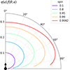 |
Fig. 1. Luminosity angular pattern η(a)f(θ; a) for different spin values. |
In order to quantify the degree of anisotropy as a function of the BH spin, we define an effective semiopening angleθeff(a), as the truncation angle of the corresponding isotropic emission such that its angle-integrated output equals that of the actual angle-dependent emission. In Fig. 2 we show θeff(a) together with η(a). From this figure we see that we have a smaller θeff, i.e, a more collimated and anisotropic angular pattern, for low spin values, whereas the radiation distribution is more isotropic (larger θeff ≃ 90°) for high spin values. Similarly, from Fig. 1 we see that in spin close to zero, the radiative flux is vertically focused along the spin axis and it decreases with increasing θ. On the other hand, the flux reduction for high θ ≲ 90° becomes less pronounced for increasing spin values, i.e., the flux collimation decreases moving towards a nearly isotropic radiation pattern.
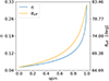 |
Fig. 2. Radiative efficiency (left y-axis) and the effective radiation semiopening angle (right y-axis) as a function of the spin parameter a. |
2.2. AGN feedback
As Ishibashi et al. (2019) and Ishibashi (2020) pointed out, if the radiation from the accretion disk couples to the surrounding material by exerting radiation pressure on dust or by launching line-driven AGN winds, then the emerging outflow inherits the anisotropy of the impinging radiation, which, in turn, it is shaped by the BH spin. This outflow spin-dependent anisotropy can affect the outflow ability to couple with the ISM and hence it may change the impact that AGN feedback has on the host galaxy and on the MBH growth. In this way, the MBH spin, through its influence on AGN feedback, can possibly play a role in the MBH-galaxy host co-evolution.
Galactic AGN driven outflows in the so-called quasar mode are typically described as the result of the interaction between the disk radiation with the surrounding material and with the transfer of energy and momentum to it. Many works assume that this coupling occurs at the scale of the accretion disk and broad line region (BLR), launching an AGN wind that mediates the interaction between the AGN radiaton and the ISM (King 2003; Zubovas & King 2012; Faucher-Giguère & Quataert 2012; Costa et al. 2014, 2020; Hartwig et al. 2018; Torrey et al. 2020). Another possibility is that the radiation escapes the inner region and couples at the ISM scale directly through radiation pressure on dust (Murray et al. 2005; Ishibashi & Fabian 2015; Thompson et al. 2015; Costa et al. 2018; Barnes et al. 2018). In the following we are going to focus on the first mechanism; that is, AGN-wind-driven outflows.
2.2.1. AGN winds
Observations of bright quasars with blueshifted X-ray absorption lines (Pounds et al. 2003; Reeves et al. 2009; Tombesi et al. 2015) give strong evidence for intense winds from galactic nuclei characterized by relativistic velocities. Such winds are believed to be launched by Thompson scattering or line-driven momentum transfer of AGN radiation to the gas. If each photon emitted by the AGN interacts just once with the gas, then the transferred momentum flux equals the radiation momentum flux L/c. If the gas is dusty, then the optical and ultraviolet (UV) radiation is absorbed and re-emitted at infrared (IR) wavelengths. If the gas is optically thick in the IR, instead of streaming out, the reprocessed IR photons undergo multiple scatterings. In this case, the net momentum imparted by the AGN radiation field may exceed L/c. More generally we indicate with τL/c the momentum transferred to the gas, where the parameter τ holds the information concerning the radiation-gas coupling and τ = 1 (> 1) in the single(multi)-scattering scenario. Then, the total momentum carried by the wind can be written as
 (3)
(3)
Using Eq. (2) and by writing the momentum loading as  , where
  is the wind momentum flux in the direction θ at a distance r from the AGN, Eq. (3) yields
 (4)
(4)
That is, the momentum flux of the wind follows the same angular pattern of the radiation. Assuming that the wind is launched at a constant velocity vw, then the mass flux in the direction θ is simply  , and hence the mass flux angular distribution of the wind follows the same angular pattern as well. By combining Eqs. (1) and (3) instead we obtain the total mass loading:
 (5)
(5)
where we define the mass loading factor,
 (6)
(6)
2.2.2. Wind-driven outflows
The further evolution of wind-driven outflows has been discussed in many papers (Weaver et al. 1977; Koo & McKee 1992; King 2003; Costa et al. 2014; Hartwig et al. 2018) and textbooks (Dyson & Williams 1997), in the context of both stellar and AGN feedback. We briefly review some aspects here.
Once launched, the AGN wind moves in the ambient medium shovelling the material it encounters along its path, forming a shell expanding at constant velocity ∼vw. This phase is referred to as free-expansion and lasts approximately until the swept-up mass equals the mass of the impinging wind. If the ambient medium has uniform density ρ0, the free expansion timescale reads
 (7)
(7)
When the shell radius reaches a distance of ∼Rfree ≡ vwtfree, the momentum of the material added to the shell start causing it to slow down significantly and free-streaming brakes down. From now on, the incoming wind forms a strong reverse shock against the slowing down shell and a significant fraction of the wind kinetic energy is thermalized. We can now distinguish a four-layers structure formed by the AGN wind, the shocked wind, the shocked ambient medium and finally the unperturbed eniviornment. The dynamics of this structured shell, or outflow, has been studied extensively both theoretically (Weaver et al. 1977; Koo & McKee 1992; Dyson & Williams 1997; Faucher-Giguère & Quataert 2012; Zubovas & King 2012; King & Pounds 2015) and numerically (Costa et al. 2014, 2020). In a nutshell, the subsequent evolution of the outflow depends on the ability of the shocked wind to preserve its thermal energy, which in turn depends on the cooling processes involved and on the associated timescales. If radiative losses in the shocked wind are negligible, it expands adiabatically doing “PdV” work on the shocked ambient medium, driving an “energy driven” outflow (King 2005). If the shocked wind is radiatively cooled, the shell of swept-up ambient gas is driven solely by the wind’s ram pressure (King 2003). Such solutions are termed “momentum driven”. If the shocked wind does cool, but inefficiently, the wind solution is intermediate between momentum and energy-driven (Faucher-Giguère & Quataert 2012).
From an observational point of view, both energy and momentum driven outflows have been detected (Fluetsch et al. 2019; Tozzi et al. 2021). However, the observed outflows are mostly on kiloparsec (kpc) scales, while theoretical arguments (Faucher-Giguère & Quataert 2012; King & Pounds 2015) and the lack of observational evidence of cooling wind shocks (Bourne & Nayakshin 2013) suggest that under realistic circumstances the shocked wind bubble cools inefficiently, and that momentum-driven outflows should be confined within the central few 100 pc from the MBH. Therefore, outflows observed in the momentum driven regime are more consistent with a radiation pressure on dusty gas mechanism or with an energy-driven outflow poorly coupled with the ISM, rather than with an efficiently cooling wind-driven outflow.
2.2.3. Energy and momentum outflows driven by anisotropic winds
We now describe how we derive the analytic solution for the propagation in a homogeneous medium of an outflow driven by an anisotropic wind, both in the energy- and momentum-driven scenarios. We characterize the evolution of the outflow by calculating the location R(θ, t) of the contact discontinuity that separates the shocked wind from the shocked ambient medium (see Fig. 3). In the energy driven regime, the shocked wind shell is hot and thick and its thermal energy evolution is due to the energy injected by the wind (suddenly converted in thermal energy) and the work done on the above shocked ambient medium. Using Eqs. (1) and (5), we have that the thermal energy is added to the shock wind layer at a rate  , where ϵ = 1/2τvw/c. Now, if we consider a single slice of the outflow, in the direction θ and subtended by a solid angle ΔΩ, as in Fig. 3, then the impinging disk luminosity in the slice direction is Lf(θ, a)ΔΩ/4π (see Eq. (2)) and a fraction ϵ of it is converted in thermal energy in the shocked wind layer of the slice. Then, if P is the pressure of the shocked wind layer, the pressure force exerted on the layer above can be written as PΔΩR2 and the PdV work as PΔΩR2dR. Assuming that the shocked wind layer is thick enough to neglect the portion of the slice occupied by the freely streaming wind, its volume can be approximated with that of the slice up to R, i.e. ΔΩR3/3, and hence its internal energy with (3/2)PΔΩR3/3. Then, if ρ0 the ambient medium density we can write the conservation of the shocked wind energy and the conservation of the shocked ambient medium momentum of the slice as
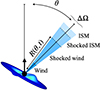 |
Fig. 3. Schematic view of the outflow structure in a slice subtended by a solid angle ΔΩ and centered in a direction forming an angle θ with the MBH spin. This stratified structure comprises the AGN wind, the shocked wind (which extends up to a distance R(θ, t) from the MBH), the shocked ISM, and the unperturbed ISM. The illustration also shows the warped accretion disc that feeds the spinning MBH. |
 (8)
(8)
 (9)
(9)
respectively. By solving Eq. (9) for P and replacing in Eq. (8) we get
 (10)
(10)
which admits the self-similar solution
 (11)
(11)
Equation (11) describes the evolution of the contact discontinuity in time, for each direction θ, in the energy driven regime.
In momentum-driven outflows, the energy of the shocked wind is quickly dissipated on small scales via radiation losses and the shocked wind shell collapses into a thin layer, as its thermal pressure support is radiated away. Then, the shocked ambient medium layer is driven outward directly by the ram pressure of the impinging AGN wind, which equals the momentum flux of the disk radiation if τ = 1. In this case, we write the momentum conservation of the shocked ambient medium in the slice as
 (12)
(12)
which is solved by
 (13)
(13)
Equation (13) represents the evolution of the contact discontinuity in the momentum driven regime. We briefly mention that the main cooling process that could make this regime possible is the Compton cooling of free electrons in the shocked wind shell against the AGN photons, as discussed in King (2003), Faucher-Giguère & Quataert (2012), Hartwig et al. (2018), Richings & Faucher-Giguère (2018), Costa et al. (2020), Torrey et al. (2020). Following Sazonov et al. (2004), if we assume that the AGN radiation field has a nearly obscuration-independent Compton temperature TAGN = 2 ⋅ 107 K, the gas Compton heating/cooling rate for gas with temperatures T < 109 K (non relativistic regime) is
 (14)
(14)
where T is the gas temperature, me the electron mass, σT the Thompson cross-section, ne the electron number density (bound + free) and r the distance of the gas element from the AGN.
3. Feedback implementation
In order to investigate the role of anisotropic radiative feedback in more realistic scenarios, we implemented the anisotropic spin-dependent AGN wind discussed above (Sect. 2.2.1) in the code GIZMO (Hopkins 2015). In a nutshell, our implementation is characterized by a subgrid accretion disk whose properties (mass Mα and angular momentum Jα) evolve due to the accretion Ṁin from resolved scales on the subgrid disk (modeled with a modified Bondi-Hoyle prescription similar to Tremmel et al. 2017) and due to the accretion Ṁacc within the subgrid disk on the MBH. Similarly, the physical (subgrid) MBH is characterized by its mass M• and its angular momentum J• and they evolve according to the subgrid accretion. This model, based on Cenci et al. (2021) and Sala et al. (2021) (see also Fiacconi et al. 2018), tracks the exchange of angular momentum between the MBH and the subgrid disk due to both the accretion on the MBH and the Bardeen-Petterson torque (Bardeen & Petterson 1975), in this way following the MBH spin evolution consistently with evolution of the subgrid disk properties. More details about the accretion and spin evolution models are provided in Appendix A.
In the following we present our AGN feedback model, based on the wind-spawning technique1 developed by Torrey et al. (2020), whose approach is similar to that devised by Costa et al. (2020) for AREPO. Contrary to the AGN feedback models based on thermal/kinetic energy injection in the gas particles neighboring the MBH, Torrey et al. (2020) and Costa et al. (2020) directly inject the wind mass, momentum, and energy from a subgrid region into the resolved scales and let the thermalisation of the wind arise naturally from the hydrodynamic evolution. While in these models the wind injection is assumed isotropic, here we force the wind momentum (Eq. (4)) and mass fluxes to follow the subgrid disk luminosity angular pattern resulting from gravitational bending, which is ultimately set by the MBH spin. We mention that another source of AGN feedback anisotropy does exist when AGN winds are accelerated at relativistic velocities. Indeed, an isotropic AGN radiation source driving a nuclear wind with relativistic velocity is perceived as anisotropic by the wind gas itself due relativistic beaming (Luminari et al. 2020). However, this effect translates into angular variations of vw of a few percent for vw = 0.01c, as we assume below, which is negligible compared to the variation in the wind momentum attributed to the photons gravitational bending.
Overall, the MBH mass and spin are evolved in a subgrid fashion according to the properties of the subgrid accretion disk, which are influenced by the resolved accretion flow on the subgrid system. The presence and characteristics of such an inflow are affected by the feedback magnitude and anisotropy, which in turn are set by the subgrid disk and MBH properties. This results in a complex nonlinear interplay between MBH fueling, feedback, its anisotropy and the MBH spin, which our subgrid model is aimed to capture. In the following we provide more details about the wind launching implementation.
Following Torrey et al. (2020) and Costa et al. (2020), we assume that a factor τ of the radiation momentum flux is transferred to the gas at subgrid scales, generating an AGN wind which is directly injected into the resolved scales. The wind mass outflow rate Ṁw is computed from the unresolved disk accretion rate as shown in Eq. (5), where both vw and τ, appearing in the definition of ηw (Eq. (6)), are free parameters of the model. In practice, the wind is simulated by removing mass from the subgrid disk and by spawning Nw new gas particles at a rate Ṁw. The newborn wind particles are distributed uniformly on a sphere centered on the MBH and with radius equal to the minimum between one tenth of the MBH gravitational softening ϵ• and half of the smallest MBH-gas particle separation. The mass distribution of the spawned particles follows the subgrid disk luminosity angular pattern. More precisely, the mass of the i−th spawned particle, with polar angle θi from the MBH spin direction, is assigned as
 (15)
(15)
where the sum at denominator spans over all the spawned particles, Mspwn is the total mass to be spawned and f(θ, a) is the luminosity angular pattern defined in Eq. (2).
The wind particles are then launched radially outward with constant velocity vw and by interacting with the other surrounding gas particles they generate an outflow. During their evolution, the wind particles can be merged into nonwind (or ISM) gas particles, properly transferring to them their mass, momentum, and energy as in an inelastic collision; see Appendix E of Hopkins (2015). We required that such a merger occurs once the velocity of the target wind particle falls below five times the mean velocity of the nonwind particles in its kernel. We provide more details about wind particles mass resolution and their merger to nonwind particles in Appendix C. In order to track the propagation of the wind into the environment, we introduced a scalar wind tracer ζ, similarly to Costa et al. (2020), that represents the wind mass fraction of a gas particle. Therefore ζ = 1 for wind particles, nonwind particles are initialized with ζ = 0 and 0 < ζ < 1 values characterize nonwind particles that experienced mergers with wind particles.
In order to be able to capture the formation of a momentum-driven outflow our model includes gas Compton cooling. We assume that the AGN photons interact with the surrounding gas at subgrid scale, launching the AGN wind, and then they are remitted isotropically. Then, such reprocessed photons can scatter with the high-energy electrons of the shocked wind layer of the outflow, making it lose energy and cool. In practice, following (Hopkins et al. 2016), a contribution ΛCpt as in Eq. (14) is included when computing radiative cooling or heating of gas particles, where r is now the distance between the gas particle and the MBH and L is the instantaneous subgrid disk luminosity computed from Eq. (1).
In the subgrid model described in the present section, the MBH time step dt• is taken to be small enough to resolve the subgrid accretion, wind launching and spin evolution and large enough to guarantee that the disk attains a steady-state warped profile, as assumed in our prescriptions (Cenci et al. 2021).
4. Tests
In order to compare the simulated evolution of the wind-driven outflows against the analytical predictions given by Eqs. (11, 13), we first adopt an idealized setup. We consider an active MBH embedded in a gas with uniform density and temperature, so to ensure that the outflow anisotropy is the result of the intrinsic anisotropy of the wind, rather than of the ambient density distribution. In order to compare the simulated outflows with Eqs. (11, 13), we switch off gravitational forces and gas self-gravity so that the outflow evolution is purely hydrodynamical. For the entire duration of the simulations, we keep the AGN luminosity and angular pattern constant; that is, we force the properties of the subgrid disk and MBH to remain constant.
In order to test both energy- and momentum-driven outflows, we consider two different setups. In the first case, we assume a gas number density μn = 1 cm−3, where μ is the mean-molecular-weight, and a MBH mass 107 M⊙, while in the second μn = 106 cm−3 and MBH mass 1010 M⊙. In both cases the gas temperature is set at T = 2 ⋅ 104 K. In order to test different outflow anisotropies, for each setup we consider three different values of the MBH spin, a• = {0.01, 0.95, 0.9982}. In the energy-driven simulation with a• = 0.01, we assume  (where
  is the Eddington accretion rate), while fEdd = 0.3 in the corresponding momentum-driven simulation. In the simulations with higher MBH spin, we keep the same subgrid disk properties as for a• = 0.01, and therefore the corresponding fEdd values scale as η(a•)/η(a• = 0.01), according to Eq. (A.6). Energy-driven simulations run up to tend ∼ 0.22 Myr, while momentum-driven ones for tend ∼ 1.5 Myr. The values of the main parameters of all runs are summarized in Table 1.
Parameters of test simulations.
Figure 4 shows the final snapshots for all six simulations, with energy-driven runs in the top panels and momentum-driven in the bottom ones. For each snapshot, the figure reports the density, temperature and pressure fields in units of the corresponding quantities of the background medium as well as well as the wind mass fraction. Superimposed to all maps, we draw as a black curve the location Rsh(tend, θ) of the contact discontinuity, as computed via Eqs. (11, 13). In the energy-driven simulations (top panels) the typical stratified structure of outflows can be recognized, with the free propagation wind layer, the shock wind, the shocked ambient medium and the unperturbed ambient medium. The simulated location of the contact discontinuity approximates very well its theoretical prediction (Eq. (11)). In the momentum-driven simulations (bottom panels) Compton cooling makes the shocked wind layer cool and collapse, forming a thin shell that separates the free expanding wind from the unperturbed medium. Again, the location of the separating shell is in good agreement with the theoretical estimate (Eq. (13)).
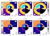 |
Fig. 4. Final snapshots of the propagation of an AGN wind-driven outflow for different spin values (increasing from left to right) and the two considered regimes (energy-driven in the top row and momentum-driven in the bottom one). Each panel illustrates the density, temperature, and pressure fields in units of the corresponding quantities of the assumed background medium as well as the wind mass fraction. In the energy-driven simulations, the outflow can be divided into four distinct sections: (1) the freely expanding wind, (2) the shocked wind, (3) the shocked ambient medium, and (4) the undisturbed ambient medium. In the momentum-driven simulations, radiative cooling makes the shocked wind layer cool and regions (2) and (3) are condensed into a thin shell. The wind tracer is injected together with the wind and is therefore only present in regions (1) and (2). The black lines correspond to the analytical location of the contact discontinuity between regions (2) and (3), as computed in Eqs. (11)–(13). In momentum-driven simulations, the cyan dashed lines indicate the effective aperture of the radiation as defined in Sect. 2.1. |
In both energy- and momentum-driven simulations, as the spin increases, the angular pattern of the emerging outflow becomes more spherical and spreads at larger distance from the MBH. This is expected, as larger spin values yield more isotropic luminosity angular patterns as well as more luminous disks.
5. Isolated galaxy simulations
We employ now the subgrid model for spin-dependent AGN winds described in Sect. 3 to study the role of wind anisotropy in shaping AGN-driven galactic outflows, and then the impact such outflows have on the host galaxy. We start by constructing an isolated galaxy setup similarly to Costa et al. (2020). We first initialize a gaseous halo of mass Mg = fgM200, where M200 = 1012 M⊙ is the halo (dark matter + gas) virial mass and fg = 0.17 the gas mass fraction, with a Navarro–Frenk–White (NFW; Navarro et al. 1997) density profile. A M• = 108 M⊙ MBH is placed at the center of the system and the gas internal energy is set to guarantee hydrostatic equilibrium in the absence of cooling. The pressure profile has been computed numerically from the gas density and total potential profiles. The halo concentration parameter is 𝒞 = 7.2, which gives a halo scale radius ahalo = 28.54 kpc and a virial radius r200 = 𝒞ahalo = 205.5 kpc. The gas initial specific angular momentum follows a profile j(r, θ), where r and θ are the spherical radial and polar coordinates, as in Eqs. (12)–(15) of Liao et al. (2017). Such profile is characterized by the halo spin parameter λsim, introduced by Bullock et al. (2001) (their Eq. (5)), which is set to λsim = 0.035.
Radiative cooling is modelled as described in (Hopkins et al. 2018), assuming initial metallicity 0.1 Z⊙ and ignoring radiative cooling processes below T < 104 K. Due to the loss of pressure support following radiative cooling, at t = 0 the spinning gaseous halo starts to collapse towards the center and the inner region settles into a galactic disk continuously fed by the outermost falling layers. We emphasize that this initial gas inflow and the subsequent galaxy formation and star formation history are sensitive to the initial halo density profile. In particular, a NFW profile, as assumed here, is likely to enhance these processes compared to other shallower profiles; see for example (Miller & Bregman 2013, 2015).
The gaseous halo is sampled with N = 3 ⋅ 105 particles only up to a radius of 0.6 r200. We note that the presence of a sharp pressure gradient at 0.6 r200 causes an artificial outflow. Nonetheless, this occurs on spatial scales far away from those considered in our analysis, which focus on the central ∼10 kpc region. In addition, the radius of 0.6 r200 within which we sample the gas is tailored to ensure that over the simulated time the boundary effects of this sampling cannot propagate within the central region of interest, as gas particles above 0.6 r200 take more than ∼0.7 Gyr to fall within ∼5 kpc from the center of the system. The mass resolution of our simulations is mgas = 3.44 ⋅ 105 M⊙. Dark matter is not sampled and enters the simulation as a static analytic potential.
Star formation is treated following Springel & Hernquist (2003), where the effects of unresolved physical processes operating within the interstellar medium (ISM) are captured by an effective equation of state that is applied to all gas with hydrogen number density nH > nth. This effective equation of state is stiffer than that of isothermal gas, because it accounts for additional pressure provided by supernova explosions within the ISM. Stellar particles are spawned stochastically from gas with nH > nth at a rate
 (16)
(16)
where β = 0.1 is the mass fraction of massive stars assumed to instantly explode as supernovae, ρc is the density of cold clouds (see Springel & Hernquist 2003, for details) and t⋆ = t⋆, 0(nH/nth)−1/2 is the star formation timescale, with t⋆, 0 = 1.5 Gyr and  . Supernova-driven winds are not modelled, as they would add a further layer of complexity affecting both star formation, the MBH growth and hence AGN feedback (see, e.g., Dubois et al. 2015). Therefore, our simulations should be regarded as idealized experiments aimed at illustrating how AGN wind modeling affects the impact of MBH feedback on the host galaxy and on the MBH evolution, without “contamination” from supernova-driven winds.
After the first 150 Myr, once a galactic disk has formed and star formation has already reached its peak, MBH accretion and feedback are “switched on”. At this instant, which we denote with t0, the gas and stellar mass of the galaxy are, respectively, ∼8.2 ⋅ 109 M⊙ and ∼7.5 ⋅ 109 M⊙. Then, we perform six different simulations divided in two sets (labelled with qcrC and qcrE) corresponding to different MBH accretion prescriptions, each set consisting of three different simulations characterized by different feedback anisotropies (indicated with labels qcrf, qcriso, qcra0). In the simulation set labelled with qcrC, the subgrid accretion disk is forced to maintain the same properties for the entire duration of the simulations, i.e., the disk mass and angular momentum do not change because of accretion onto the MBH and wind ejection. In these simulations, the Eddington factor  is kept constant equal to 1 (similarly to Torrey et al. 2020; Costa et al. 2020 and Mercedes-Feliz et al. 2023), corresponding to a subgrid disk of constant luminosity L = 1.2 ⋅ 1046 erg/s. On the contrary, in qcrE simulations, fEdd is allowed to evolve and its value is set by the instantaneous MBH + subgrid disk properties (Eq. (A.6)), which, in turn, are determined by the inflow on the disk, the accretion on the MBH and wind ejection (see Eqs. (A.1)–(A.4)). In this way, qcrE-simulations are able to capture the mutual nonlinear influence that inflows and outflows have on each other and that lead to self-regulated MBH growth2. In addition to these simulation sets, we prolonged the simulation for the spinning halo collapse beyond 150 Myr without switching on the AGN, so that the sets qcrC and qcrE can be compared to the case in which the MBH is not active. We indicate this simulation with qcrNoFb.
Both qcrC and qcrE sets consist of three simulations, accounting for a different wind anisotropy. Simulations qcrf have an angular pattern f(θ; a), as illustrated in Sect. 2.1; this pattern evolves according to the evolution of the spin parameter a; qcriso-simulations are characterized by an isotropic angular pattern, i.e. f = 1; qcra0-simulations assume instead a fixed angular pattern corresponding to the one of a ≃ 0, f = f(θ; 0.01). We note that, independent of the anisotropy pattern, the MBH spin and η(a) are allowed to evolve in these runs. The motivation for these choices of angular patterns is the following: real outflows anisotropy can result from the wind “intrinsic” anisotropy imparted by the radiation angular pattern and linked to the MBH spin, i.e. the anisotropy discussed in Sect. 2.1 and seen in Fig. 4, or it can be induced by the anisotropy of the medium in which the outflow propagates as, for example, in a spiral galaxy where the gas density is higher in the midplane of the galaxy than perpendicular to it. In this way, an “intrinsically” spherical outflow expands more easily along the galaxy axis, i.e., along the least resistance path, turning into a bipolar (anisotropic) outflow (Hartwig et al. 2018; Costa et al. 2020; Zubovas & Maskeliūnas 2023)3. Since outflow anisotropy is shaped by these two factors, both present in simulations qcrf, a comparison with simulations qcriso allows to disentangle these effects and to properly assess the relevance of radiation pattern anisotropy in galactic outflows. Instead, simulations qcra0 represent the opposite term of comparison, in which the angular pattern is maximally anisotropic, i.e. f(θ; 0.01)≃2cosθ as in (Newtonian) α-disks, as if all the isotropy coming from gravitational bending were removed. We summarize the main features of the six simulations performed in Table 2.
Isolated galaxy simulations suite.
In both qcrC and qcrE sets, we start the simulations at t0 with fEdd = 1, a = 0.01, Mα = 0.005M• and M• + Mα = 108 M⊙. The wind velocity and temperature are fixed to vw = 0.01 c and Tw = 2 ⋅ 104. Nw = 48 wind particles are spawned at each spawning event and the radiation-wind coupling parameter is fixed to τ = 1. In all simulations the gravitational softening for all particle species is 2 pc.
In the following subsections, we discuss the impact of AGN feedback in our setups, focusing on the one hand on its effect on the host galaxy, in particular on the central gas reservoir and star formation, and on the other hand on its influence on the MBH evolution in mass and spin. Before entering into detail, we provide a qualitative glimpse of how the galaxy–MBH evolution appears in simulations qcrC_f and qcrE_f.
Figure 5 shows three snapshots of the simulation qcrC_f, both face on (top panels) and side-on (bottom panels). In the side-on view, we see that after t ≃ 8 Myr from the AGN “switch on”, a collimated wind is piercing the circumgalactic medium (CGM), its opening angle widening over time. Correspondingly, in the face-on view, a ∼kpc-scale cavity is cleared in the central region surrounding the MBH, becoming increasingly large with time. Both these effects are accompanied by an increase of the spin value, which reaches ∼0.998 after ≃64 Myr, and hence by an increase in the disk radiative efficiency and in the isotropy of the radiation angular pattern (see discussion in Sect. 2.1). We remark that in this simulation the accretion rate on the MBH is forced to be constant, equal to the Eddington rate. However, as noted by Torrey et al. (2020), once the gas reservoir feeding the MBH diminishes with the formation of a central cavity, the accretion on the MBH should decrease as well, reducing the AGN power and hence its ability to further enlarge the cavity. We show this effect in Fig. 6, which is the analogous of Fig. 5 for the simulation qcrE_f, in which the MBH accretion is consistently evolved with the inflow on the disk and the wind ejection from it. In this case, no cavity formation can be seen in the face-on view and a milder wind (compared to Fig. 5) is seen in the side-on view. This suggests that a much lower accretion (and hence outflow) rate is achieved once that the disk is allowed to adjust itself through its interaction with the environment. In particular, we see in Sect. 5.1.1 that, in this simulation, fEdd indeed drops by between one and two orders of magnitude from its initial value.
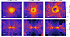 |
Fig. 5. Density slices of three snapshots from simulation qcrC_f, with the disk face-on in the top panels and side-on in the bottom panels. The MBH location is marked by a black dot. |
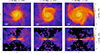 |
Fig. 6. Density slices of three snapshots from simulation qcrE_f, with the disk face-on in the top panels and side-on in the bottom panels. The MBH location is marked by a black dot. |
In Figure 7 we show a zoom-out of the side-on view of simulation qcrE_f at t = 24 Myr. The four columns illustrate, from left to right, the gas density, the wind mass fraction, the gas internal energy, and the electron abundance fraction ne/nH. Even though the AGN wind does not seem to affect much the host galaxy (Fig. 6), it propagates deeply in the CGM creating a hot, low-density, ionized bipolar outflow that extends in the polar directions and regulates the inflow onto the galaxy, hence its growth.
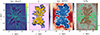 |
Fig. 7. From left to right, edge-on maps of the gas density, the wind mass fraction, the internal energy, and the electron abundance fraction of simulation qcrE_f at t = 24 Myr. |
We now discuss more quantitatively the impact of feedback both on the MBH and the galaxy host, turning our attention to the relevance of the spin-dependent wind anisotropy.
5.1. The impact of AGN feedback on the MBH
In order to understand how the MBH mass and spin evolve and to what extend their growth is influenced by AGN feedback, we need to understand its back-reaction on fEdd, which characterizes the rate of such growth.
5.1.1. Evolution of fEdd
In qcrC simulations, the growth of MBH mass and spin is completely determined by the constrain fEdd = 1, so it is independent on any effect feedback might have on the gas surrounding the MBH. Conversely, in qcrE simulations, fEdd varies with time according to the evolution of the subgrid disk+MBH system (Eq. (A.6)), which is influenced by the action of feedback on the nuclear environment. Indeed, in this case, AGN feedback diminishes the gas density in the vicinity of the MBH, lowering the mass inflow rate on it and hence the AGN power.
In order to have a better understanding of how fEdd evolves, we compute the time derivative dfEdd/dt (see Appendix A.2), finding that it can be approximated as
 (17)
(17)
where Ṁin is the mass inflow rate on the subgrid disk from resolved scales, as defined in Appendix A.1, and the coefficients Cw and Cin are both found to be ≃0.1, as detailed in Appendix A.2. Equation (17) describes the evolution of fEdd as driven by the disk mass loss, proportional to Ṁw, and by the inflow Ṁin that supplies mass to the disk; in other words, the disk accretion rate is regulated by the balance between outflows and inflows. Because of the different signs in front of Cw and Cin, the disk tends to evolve towards a stationary dfEdd/dt ∼ 0 regime. Indeed, if the inflow exceeds the outflow, i.e.  , then the accretion rate fEdd increases and Ṁw grows as well (see Eq. (5)). By contrast, if the disk mass consumption outpaces the external mass supply,
  , the accretion rate decreases and hence Ṁw diminishes too. In this way inflows and outflows tend to adjust each other such that
  , i.e. dfEdd/dt ∼ 0.
Figure 8 shows the evolution of Ṁw and Ṁin in the three simulations qcrE and reveals that in all cases  and both quantities settle around ∼1 M⊙/yr after a transient of ∼50 Myr. As a result, in all qcrE simulations, fEdd decreases from its initial value fEdd, 0 = 1 and, after ∼50 Myr, attains a value ∼0.05 (see Fig. 9), which is consistent with observed Seyfert galaxies (Ho 2009) and corresponds to a moderate luminous AGN with L ≃ 6 ⋅ 1044 erg/s.
 |
Fig. 8. Evolution of the mass inflow rate Ṁin on the subgrid disk and the mass outflow rate Ṁw ejected in winds for the three qcrE simulations. The solid and dashed lines correspond to the median values of these quantities over time bins of 5 Myr, while the shaded regions span from the 16th to the 84th percentiles of Ṁin and Ṁw within the bins. |
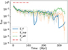 |
Fig. 9. Evolution of fEdd in qcrE and qcrC simulations. The lines correspond to the median values of fEdd over time bins of 5 Myr, while the shaded regions represent the fluctuations within the bins from the 16-th to 84-th percentiles. |
5.1.2. MBH mass and spin growth
The mass and spin evolution of the MBH in all our simulations is shown in Figure 10. In qcrC simulations, the growth of MBH mass and spin is constrained by fEdd = 1, whereas in qcrE simulations fEdd varies with time (Fig. 9), according to the interplay between inflows and outflows, as discussed in 5.1.1. In this second case fEdd lowers down to ∼0.05, in this way the MBH mass and spin growth is severely delayed compared to the fEdd = 1 case.
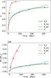 |
Fig. 10. MBH spin and mass growth in qcrE and qcrC simulations. The red and blue bullet points mark the instants corresponding to the snapshots shown in Figures 5 and 6. |
While the disk luminosity is directly linked to the MBH mass and spin growth rates (Eq. (1)), its angular pattern has a negligible impact on them. Nonetheless, in qcrE simulations we notice a small dependence of these growth rates with the radiation angular pattern, i.e. the more isotropic the angular pattern is (where isotropy rises with qcra0 → qcrf → qcriso), the slower the mass and spin growth is. This can be attributed to the wind-ISM coupling increasing with isotropy (see Sect. 5.2), thus yielding smaller mass inflow rates on the MBH and hence lower AGN power.
5.2. The impact of AGN feedback on the galaxy host
We now quantify the impact of AGN feedback on the host galaxy by probing the galaxy star formation history, the size of the central cavity, the AGN wind opening angle and the CGM properties.
5.2.1. Star formation rate history
In Figure 11 we show the evolution of the star formation rate (SFR) with time. In order to differentiate the effect of the AGN feedback on nuclear and galactic scales, in the left panel we consider the SFR of the gas particles within 0.5 kpc from the MBH, while in the right panel the SFR of the gas particles within 5 kpc. In both panels, we show results from the simulations sets qcrC and qcrE and from simulation qcrNoFb that with no feedback.
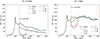 |
Fig. 11. Star formation rate in the nuclear region (left) and at galactic scale (right) for qcrE, qcrC, and qcrNoFb simulations. Here, t = 0 corresponds to the initial condition with the spinning gaseous halo in hydrostatic equilibrium and t0 = 150 Myr (when AGN feedback is turned on) is marked with a gray vertical line. |
The qcrNoFb simulation traces the evolution of the SFR starting from the initial condition with the spinning halo in hydrostatic equilibrium. At this time the SFR is zero, but as soon as the gaseous halo collapses, getting denser and cooler, the SFR grows and peaks at ∼100 Myr, both on nuclear and galactic scales. At this point, while in the central region the SFR starts to decline, in the whole galaxy stars continue to be formed at a rate of 100 M⊙/yr ÷125 M⊙/yr. The switch-on of AGN feedback at t0 = 150, in qcrC and qcrE runs, modifies these trends. In the central 0.5 kpc, the SFR is reduced by a factor of ≲2 in qcrE simulations, while it is completely shut off in qcrC simulations. The imprint of AGN feedback on galactic scales is less marked: in qcrE-simulations the SFR within 5 kpc is not appreciably altered, except for a ≲20% decrease during the first ∼50 Myr of AGN activity, and a burst of SFR at the end of qcrE_iso due to a clump in a spiral arm, whereas it diminishes by a factor of ≲2 in qcrC runs. Overall, these trends do not show any significant dependence on the AGN radiation angular pattern, except for qcrC simulations at galactic scale. In this case, we see that the more isotropic the luminosity angular pattern is, the more the SFR is suppressed, due to the increase of wind-ISM coupling. However, this appears as a second order effect and the impact of AGN feedback on the SFR is mainly driven by the AGN luminosity, rather than by its angular pattern.
5.2.2. The size of the central cavity
The trends seen in the SFR history are closely related to those seen in the size of the central cavity cleared by AGN feedback. Here the cavity size is measured as the radius Rcav of the sphere centered in the MBH containing a gas mass equal to the MBH mass. Figure 12 shows that in the simulation without feedback this quantity is initially (at t0) about 50 pc and overall grows up to ∼100 pc. In simulations with AGN feedback, AGN winds tends to push the gas away from the MBH, lowering the gas density in its surroundings and thus increasing Rcav. Such an increase is modest in qcrE simulations, by a factor less than 2, while it is about an order of magnitude larger in qcrC simulations. In this second case, we can distinguish a dependence of the cavity size with the feedback radiation angular pattern, where a more isotropic pattern results in a larger cavity.
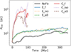 |
Fig. 12. Evolution of the central cavity size in qcrE, qcrC, and qcrNoFb simulations. |
As for the SFR, the cavity size seems to be determined at first order by the disk luminosity and only for high (Eddington) luminosities (qcrC runs) by the radiation angular pattern, at least partially. In addition, the increase in the cavity size with disk luminosity and with disk radiation angular pattern mirrors what we found for the SFR, i.e., larger cavities are associated with lower SFRs. This suggests that star formation suppression in the galaxy nuclear region occurs via gas removal caused by AGN winds.
5.2.3. The outflow opening angle
Now we show how we measure the opening angle of the region within which the SFR is maintained below 1 M⊙/yr, which provides information about the anisotropy (or angular amplitude) of the bipolar outflow. In order to compute this quantity, we first determined, at any time t, the SFR angular profile SFR(θ; t), where θ is the polar angle from the galaxy axis4. For all simulations, SFR(θ; t)≃10−2 ÷ 10−1 M⊙/yr for small θ – that is, perpendicular to the galaxy disk plane – and rapidly increases at θ ≳ π/3, reaching ≃10 ÷ 102 M⊙/yr for θ ≲ π/2 – that is, in the galactic disk midplane. Given this trend, we define θ⋆ as the angle below which the SFR(θ; t) < 1 M⊙/yr. Then, the larger θ⋆, the wider the angular region where the outflow manages to keep the SFR below our treshold of 1 M⊙/yr. In this sense, θ⋆ measures the outflow semiopening angle.
In Figure 13, we show how θ⋆ evolves in our simulations and we notice a trend similar to that of SFR(t) and Rcav(t). Indeed, θ⋆(t)≳π/3 in qcrNoFb simulation, then becomes larger in qcrE simulations and increases further in qcrC runs. No particular trend of θ⋆ is seen with the feedback radiation angular pattern, except for the final part of qcrC simulations, which suggest that θ⋆ is larger for more isotropic radiation angular patterns. Therefore, similarly to what we discussed for SFR(t) and Rcav(t), the disk luminosity, more than its angular pattern, determines the angular amplitude of the outflow, measured as the ability of AGN winds to hamper the SFR at large polar angles.
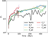 |
Fig. 13. Evolution of the outflow semiopening angle in qcrE, qcrC, and qcrNoFb simulations. |
5.2.4. The impact on the CGM
While on galactic (∼10 kpc) scales there is a mild or absent dependence of the outflow opening angle on the AGN radiation anisotropy, this is not the case if we look at the larger CGM (∼100 kpc) scales, where an imprint of the feedback anisotropy on the CGM temperature and entropy can be appreciated.
In Figure 14 we show the time averages of the CGM temperature and entropy (left and right of each panel respectively) for the three simulations in the set qcrE. Entropy is computed as K = kBTne−2/3 and the time averages only consider snapshots up to 180 Myr from t0 in order to avoid boundary condition effects caused by the finite size of the sampled halo. Fig. 14 emphasizes that while the opening angle of the outflow on a small scale does not seem to be affected by the anisotropy of the radiation emitted by the AGN, on a larger scale, the more isotropic the radiation angular pattern, the larger the volume fraction of the CGM that is affected by the outflow. This in turn can reflect in the outflow ability to prevent cooling flows on the galaxy and thus on the galaxy cold gas growth and its star formation history on longer timescales. Despite these effects on the energetics of the gas in the CGM, the radial density profile is not affected by feedback anisotropy, as illustrated in Figure 15, where the time averages of these profiles for the qcrE simulations are shown.
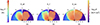 |
Fig. 14. Polar plots of the time averages of CGM temperature and entropy for qcrE simulations. Time averages are taken considering snapshots up to 180 Myr from t0. |
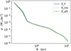 |
Fig. 15. Time averages of the density radial profile of the CGM for the qcrE simulations. |
We provide more details on the CGM energetic balance in Appendix B.
6. Summary and Discussion
In this study, we investigated the role that spin-dependent anisotropy of AGN winds (Ishibashi et al. 2019; Ishibashi 2020) has in shaping the evolution of MBHs and their host galaxies. To this purpose, we implemented – in the code GIZMO – a subgrid model for AGN feedback that takes into account the spin dependence of feedback anisotropy, linking and integrating existing modules for MBH accretion and spin evolution (Cenci et al. 2021) and AGN wind (Torrey et al. 2020). In doing so, we assumed that the AGN disk radiation couples with gas at the disk (subgrid) scale, completely transferring its momentum. In this way, the nuclear wind that is launched inherits the luminosity angular pattern of the impinging radiation, which is set by the MBH spin. We initially tested our novel implementation by following the propagation of an AGN-wind-driven outflow into a homogeneous medium, and we compared the results against simple analytical models. We then considered an isolated galaxy setup, where the galaxy is thought to be formed from the collapse of a spinning gaseous halo, and there we studied the impact of AGN feedback on the MBH and galaxy evolution. We considered different prescriptions for the MBH accretion rate – that is, constant and equal to the Eddington rate, or self-consistently evolving according to the resolved gas inflow onto the MBH. We also considered different degrees of anisotropy of the angular pattern of the launched AGN wind.
The most relevant results of our work can be summarized as follows:
-
MBH feedback and fueling are tightly intertwined. On the one hand, the AGN wind affects the gas reservoir that feeds the MBH and, on the other hand, gas flowing onto the MBH supplies material and powers the wind. The disk–wind system is a complex, self-regulating system (Fiore et al. 2024). We find that whether or not we account for such self-regulated evolution makes a crucial difference. In our simulations with an evolving MBH accretion rate, the AGN luminosity, initially set equal to Eddington LEdd = 1.2 ⋅ 1046 erg/s, drops down by between one and two orders of magnitude to ≃6 ⋅ 1044 erg/s, precisely because the AGN feedback limits the inflow that powers itself. Such reduced luminosity corresponds to an Eddington factor of fEdd ∼ 0.05, which is consistent with what is estimated in Seyfert galaxies (Ho 2009). Such a decrease in luminosity implies both a much slower MBH growth and a much weaker impact of the AGN on the host when compared with simulations with a constant Eddington MBH accretion rate. This highlights the importance of self-consistently evolving MBH accretion and feedback.
-
Once MBH accretion is allowed to evolve, we find that AGN feedback has a limited impact on the host galaxy, except for the central ≃kpc-scale region. A smaller, ≃100 pc cavity is cleared around the AGN. At the same time, the SFR is approximately halved within the inner 0.5 kpc, while it remains at values typical of inactive galaxies on larger scales. In other words, our simulations indicate that isolated disk galaxies may be able to host luminous AGN activity without undergoing any significant star formation suppression on larger galaxy scales. We emphasize that due to the simulated timescales, the star formation suppression witnessed in our simulations is the result of the AGN wind ejection of the existing ISM, while star formation suppression owing to CGM heating – which prevents cooling and accretion flow onto the galaxy – is at most mildly captured, as such processes unfold on longer, approximately gigayear timescales. Our results agree with many observational studies that find no systematic signature of AGN feedback on the host galaxy SFR (Rosario et al. 2013; Scholtz et al. 2020; Smirnova-Pinchukova et al. 2022; Lammers et al. 2023). In addition, Lammers et al. (2023) noted that AGNs, despite not showing evidence of galaxy-wide quenching, have a significantly suppressed central (∼kpc scale) SFR, lying up to a factor of 2 below those of the control inactive galaxies, in agreement with our findings. These results suggest that the integrated effect of secular AGN feedback, which is traced by the MBH mass rather than an instantaneous AGN-driven outflow, is required to significantly affect SF on galactic scales. In other words, the instantaneous AGN luminosity is not a proxy for the cumulative impact of AGN feedback on SF (Bluck et al. 2023). In addition, we recall that, in addition to AGN feedback, other physical processes can be responsible for suppression of SF in the nuclear region; for example, the presence of bars (Gavazzi et al. 2015).
-
The impact of AGN feedback on the host galaxy and on MBH growth is primarily determined by AGN disk luminosity rather than by its angular pattern. We find that MBHs accreting with a constant Eddington rate corresponding to a bolometric luminosity of L ∼ 1.2 ⋅ 1046 erg/s are capable of clearing kpc-scale cavities, suppressing SF by a factor of two on a galactic scale, and driving outflows with large – between ∼π/3 and π/2 – semiopening angles. For lower luminosities, L ∼ 6 ⋅ 1044, which are achieved once self-regulation is allowed, such effects are milder and restricted to the nuclear region. This is consistent with Torrey et al. (2020), who find that increasing luminosity allows further growth of the central cavity and suppression of SFR.
-
Conversely, the imprint of the AGN luminosity angular pattern on the MBH–galaxy evolution is less marked, and can be appreciated only in cases with high (Eddington) constant accretion rates, in which the AGN impact is stronger overall. For maximally anisotropic ∼cosθ angular patterns (our qcra0 simulations), most of the wind momentum and energy are funneled in the MBH spin direction – which is perpendicular to the galaxy disk – without sigificantly affecting the host galaxy. With more isotropic angular patterns, such as those occurring for higher MBH spin because of relativistic light bending, a larger fraction of the wind energy and momentum is distributed perpendicular to the spin – that is, into the galactic disk –, yielding a higher coupling between the wind and the galaxy ISM. Indeed, in our simulations with Eddington accretion, we observe that AGNs with isotropic luminosity more efficiently suppress the host SFR – that is, by up to a factor of two compared to the maximally anisotropic case – and more easily sweep away gas in the nuclear region, clearing cavities up to ten times larger. However, in simulations with smaller (fEdd ∼ 0.05) accretion rates, differences in the response of the galaxy to different AGN radiation anisotropies are negligible, with the exception of the CGM, on which the impact of the outflow shows small but appreciable differences with the AGN feedback angular pattern. As a consequence, we expect the spin-dependent anisotropy of AGN radiation to be relevant in those scenarios characterized by high and prolonged MBH accretion episodes and by a high opening angle of the ISM disk as seen by the central MBH, as both features would increase the wind–galaxy coupling and make the galaxy response more sensitive to the radiation angular pattern. These conditions might be satisfied during galaxy mergers, where large amounts of gas are funneled into the galactic nucleus, resulting in elevated MBH accretion rates and quasi-isotropic central gas geometries, or in high-redshift galaxies characterized by thick disks and by MBH accretion rates close to the Eddington limit over long periods of time (e.g., Di Matteo et al. 2017; Barai & de Gouveia Dal Pino 2019; Lupi et al. 2019, 2022).
-
The spin growth itself is influenced by the AGN angular pattern. Given a constant accretion rate, the spin growth naturally slows down due the distance of the ISCO from the MBH becoming smaller with increasing spin. In addition, as the spin becomes larger, both AGN luminosity and its isotropy increase and make the AGN feedback more capable of reducing the inflow on the MBH itself, further delaying its spin and mass growth. We see a hint of this trend in our simulations with self-regulated accretion, noting that more isotropic angular patterns yield slower MBH mass and spin growths; nevertheless, this effect appears negligible in our simulations. In this respect, we might speculate that, because of the angular pattern anisotropy, high-redshift slowly spinning MBHs might more easily attain accretion rates above the Eddington limit, as they would be less prone to hinder accretion flows in the AGN disk equatorial plane via winds (Lupi et al. 2016), but also because the efficiency of the jets – potentially suppressing super-Eddington accretion rates – is lower for lower MBH spins (Regan et al. 2019; Massonneau et al. 2023).
While in this paper we discuss the role of the spin-dependent anisotropy of AGN winds in the context of isolated disk galaxies, we note that this effect might be crucial in other astrophysical scenarios where AGN feedback intervenes, such as the pairing and migration of MBH binaries (e.g., del Valle & Volonteri 2018; Bollati et al. 2023). Due to our simplified modeling, there are indeed a number of caveats that we have to keep in mind when interpreting our results:
-
Our accretion model does not include the geometrically thick, radiatively inefficient accretion mode that occurs below ≲fEdd ∼ 0.01. For such low accretion rates, the disk is still modeled as an α-disk. Moreover, once the disk enters such a low accretion regime, it becomes prone to launching a jet, a phenomenon not included in our model. Due to these limitations, we are not able to capture any transition from quasar to jet mode with its possible repercussion on the host galaxy and MBH evolution. Nonetheless, this should not occur frequently given that, in our simulations, fEdd > 0.01 most of the time.
-
The coupling coefficient
 between AGN radiation and gas is assumed to be constant and equal to one. All the momentum transfer is assumed to take place at the disk (unresolved) scale with the launch of the AGN wind. In a more realistic model, the radiation–gas coupling should evolve according to the ionization level of the gas, and a fraction of the AGN radiation should be allowed to escape the unresolved disk scale and interact directly with the resolved ISM gas, exerting radiation pressure on it (Costa et al. 2018; Barnes et al. 2018). This would require radiation-hydrodynamics simulations, something we leave for future work.
 -
We did not model stellar winds and supernovae which, together with AGN feedback, contribute to driving galactic outflows, especially in dwarf galaxies (Koudmani et al. 2022), and to regulating the amount of gas present in the central region of a galaxy, thus further modulating the AGN fueling (Dubois et al. 2015; Anglés-Alcázar et al. 2017b). These effects would add a further layer of complexity – beyond the scope of this paper – that is important in order to understand the detailed interaction between star formation, MBH growth and feedback, and the overall co-evolution of MBHs and galaxies.
-
The multiphase structure of the ISM is not resolved, but is evolved in a subgrid fashion according to the (Springel & Hernquist 2003) model. An explicit modeling of the inhomogeneous and clumpy ISM structure (Hopkins et al. 2018; Lupi et al. 2019; Marinacci et al. 2019) is beyond the scope of our novel investigation of spin-dependent feedback.
We plan to address some of the caveats listed above in future work aimed at developing and enriching the subgrid model presented in this paper. Similarly, we plan to use this model to study other astrophysical regimes relevant for black holes evolution.
For the sake of completeness, we mention that the spawning particle technique has also been used with the GIZMO code in the context of stellar feedback (Grudić et al. 2021), AGN jets (Su et al. 2021), and AGN winds in zoom-in simulations (Mercedes-Feliz et al. 2023).
Torrey et al. (2020) showed that an Eddington accreting AGN generates wide cavities in its surroundings, but noted that this lower density should reflect in decreased inflow on the AGN in turn reducing his power and the cavity size itself, letting the system self-regulate.
This may explain, for example, the presence of the Fermi bubbles in the Milky Way (Zubovas & Nayakshin 2012).
We defined SFR(θ; t) as the sum of the SFR of all gas particles with polar coordinate θi ∈ [θ − Δθ/2, θ + Δθ/2], or π − θi in the same interval, and within a distance of 5 kpc from the MBH. We used Δθ = π/40.
The dynamical mass is that used in the computation of the gravitational force.
In case h• reaches it minimum value ∼2.8ϵ•, we have that Rin ∼ ϵ•.
Acknowledgments
We acknowledge the CINECA award under the ISCRA initiative, for the availability of high-performance computing resources and support (project number HP10CAKAY4). The analyses reported in this work have been mainly performed using pynbody (Pontzen et al. 2013). The data underlying this article will be shared on reasonable request to the corresponding author.
References
- Akerman, N., Tonnesen, S., Poggianti, B. M., Smith, R., & Marasco, A. 2023, ApJ, 948, 18 [NASA ADS] [CrossRef] [Google Scholar]
- Anglés-Alcázar, D., Davé, R., Faucher-Giguère, C.-A., Özel, F., & Hopkins, P. F. 2017a, MNRAS, 464, 2840 [Google Scholar]
- Anglés-Alcázar, D., Faucher-Giguère, C.-A., Quataert, E., et al. 2017b, MNRAS, 472, L109 [Google Scholar]
- Barai, P., & de Gouveia Dal Pino, E. M. 2019, MNRAS, 487, 5549 [NASA ADS] [CrossRef] [Google Scholar]
- Barai, P., Murante, G., Borgani, S., et al. 2016, MNRAS, 461, 1548 [NASA ADS] [CrossRef] [Google Scholar]
- Barausse, E. 2012, MNRAS, 423, 2533 [NASA ADS] [CrossRef] [Google Scholar]
- Bardeen, J. M., & Petterson, J. A. 1975, ApJ, 195, L65 [Google Scholar]
- Bardeen, J. M., Press, W. H., & Teukolsky, S. A. 1972, ApJ, 178, 347 [Google Scholar]
- Barnes, D. J., Kannan, R., Vogelsberger, M., & Marinacci, F. 2018, MNRAS, submitted [arXiv:1812.01611] [Google Scholar]
- Berti, E., & Volonteri, M. 2008, ApJ, 684, 822 [NASA ADS] [CrossRef] [Google Scholar]
- Blandford, R. D., & Znajek, R. L. 1977, MNRAS, 179, 433 [NASA ADS] [CrossRef] [Google Scholar]
- Bluck, A. F. L., Piotrowska, J. M., & Maiolino, R. 2023, ApJ, 944, 108 [NASA ADS] [CrossRef] [Google Scholar]
- Bollati, F., Lupi, A., Dotti, M., & Haardt, F. 2023, MNRAS, 520, 3696 [NASA ADS] [CrossRef] [Google Scholar]
- Bourne, M. A., & Nayakshin, S. 2013, MNRAS, 436, 2346 [CrossRef] [Google Scholar]
- Bower, R. G., Benson, A. J., & Crain, R. A. 2012, MNRAS, 422, 2816 [NASA ADS] [CrossRef] [Google Scholar]
- Bullock, J. S., Dekel, A., Kolatt, T. S., et al. 2001, ApJ, 555, 240 [NASA ADS] [CrossRef] [Google Scholar]
- Bustamante, S., & Springel, V. 2019, MNRAS, 490, 4133 [CrossRef] [Google Scholar]
- Campitiello, S., Ghisellini, G., Sbarrato, T., & Calderone, G. 2018, A&A, 612, A59 [NASA ADS] [CrossRef] [EDP Sciences] [Google Scholar]
- Cenci, E., Sala, L., Lupi, A., Capelo, P. R., & Dotti, M. 2021, MNRAS, 500, 3719 [Google Scholar]
- Choi, E., Ostriker, J. P., Naab, T., & Johansson, P. H. 2012, ApJ, 754, 125 [NASA ADS] [CrossRef] [Google Scholar]
- Cicone, C., Brusa, M., Ramos Almeida, C., et al. 2018, Nat. Astron., 2, 176 [Google Scholar]
- Costa, T., Sijacki, D., & Haehnelt, M. G. 2014, MNRAS, 444, 2355 [Google Scholar]
- Costa, T., Rosdahl, J., Sijacki, D., & Haehnelt, M. G. 2018, MNRAS, 473, 4197 [Google Scholar]
- Costa, T., Pakmor, R., & Springel, V. 2020, MNRAS, 497, 5229 [Google Scholar]
- Croton, D. J., Springel, V., White, S. D. M., et al. 2006, MNRAS, 365, 11 [Google Scholar]
- Curtis, M., & Sijacki, D. 2016, MNRAS, 463, 63 [NASA ADS] [CrossRef] [Google Scholar]
- Davé, R., Anglés-Alcázar, D., Narayanan, D., et al. 2019, MNRAS, 486, 2827 [Google Scholar]
- del Valle, L., & Volonteri, M. 2018, MNRAS, 480, 439 [CrossRef] [Google Scholar]
- Di Matteo, T., Springel, V., & Hernquist, L. 2005, Nature, 433, 604 [NASA ADS] [CrossRef] [Google Scholar]
- Di Matteo, T., Croft, R. A. C., Feng, Y., Waters, D., & Wilkins, S. 2017, MNRAS, 467, 4243 [NASA ADS] [CrossRef] [Google Scholar]
- Dotti, M., Volonteri, M., Perego, A., et al. 2010, MNRAS, 402, 682 [NASA ADS] [CrossRef] [Google Scholar]
- Dubois, Y., Volonteri, M., Silk, J., et al. 2015, MNRAS, 452, 1502 [Google Scholar]
- Dubois, Y., Beckmann, R., Bournaud, F., et al. 2021, A&A, 651, A109 [NASA ADS] [CrossRef] [EDP Sciences] [Google Scholar]
- Dyson, J. E., & Williams, D. A. 1997, The Physics of the Interstellar Medium, 2nd edn. (Bristol: Institute of Physics Publishing) [CrossRef] [Google Scholar]
- Fanidakis, N., Baugh, C. M., Benson, A. J., et al. 2011, MNRAS, 410, 53 [NASA ADS] [CrossRef] [Google Scholar]
- Faucher-Giguère, C.-A., & Quataert, E. 2012, MNRAS, 425, 605 [Google Scholar]
- Ferrarese, L., & Merritt, D. 2000, ApJ, 539, L9 [Google Scholar]
- Fiacconi, D., Sijacki, D., & Pringle, J. E. 2018, MNRAS, 477, 3807 [NASA ADS] [CrossRef] [Google Scholar]
- Fiore, F., Gaspari, M., Luminari, A., Tozzi, P., & de Arcangelis, L. 2024, A&A, 686, A36 [NASA ADS] [CrossRef] [EDP Sciences] [Google Scholar]
- Fluetsch, A., Maiolino, R., Carniani, S., et al. 2019, MNRAS, 483, 4586 [NASA ADS] [Google Scholar]
- Fluetsch, A., Maiolino, R., Carniani, S., et al. 2021, MNRAS, 505, 5753 [NASA ADS] [CrossRef] [Google Scholar]
- Gavazzi, G., Consolandi, G., Dotti, M., et al. 2015, A&A, 580, A116 [NASA ADS] [CrossRef] [EDP Sciences] [Google Scholar]
- Grudić, M. Y., Guszejnov, D., Hopkins, P. F., Offner, S. S. R., & Faucher-Giguère, C.-A. 2021, MNRAS, 506, 2199 [NASA ADS] [CrossRef] [Google Scholar]
- Häring, N., & Rix, H.-W. 2004, ApJ, 604, L89 [Google Scholar]
- Harrison, C. M. 2017, Nat. Astron., 1, 0165 [NASA ADS] [CrossRef] [Google Scholar]
- Hartwig, T., Volonteri, M., & Dashyan, G. 2018, MNRAS, 476, 2288 [CrossRef] [Google Scholar]
- Henden, N. A., Puchwein, E., Shen, S., & Sijacki, D. 2018, MNRAS, 479, 5385 [CrossRef] [Google Scholar]
- Henriques, B. M. B., White, S. D. M., Thomas, P. A., et al. 2015, MNRAS, 451, 2663 [Google Scholar]
- Hirschmann, M., Dolag, K., Saro, A., et al. 2014, MNRAS, 442, 2304 [Google Scholar]
- Ho, L. C. 2009, ApJ, 699, 626 [NASA ADS] [CrossRef] [Google Scholar]
- Hopkins, P. F. 2015, MNRAS, 450, 53 [Google Scholar]
- Hopkins, P. F., & Quataert, E. 2011, MNRAS, 415, 1027 [NASA ADS] [CrossRef] [Google Scholar]
- Hopkins, P. F., Torrey, P., Faucher-Giguère, C.-A., Quataert, E., & Murray, N. 2016, MNRAS, 458, 816 [NASA ADS] [CrossRef] [Google Scholar]
- Hopkins, P. F., Wetzel, A., Kereš, D., et al. 2018, MNRAS, 477, 1578 [NASA ADS] [CrossRef] [Google Scholar]
- Ishibashi, W. 2020, MNRAS, 495, 2515 [NASA ADS] [CrossRef] [Google Scholar]
- Ishibashi, W., & Fabian, A. C. 2015, MNRAS, 451, 93 [NASA ADS] [CrossRef] [Google Scholar]
- Ishibashi, W., Fabian, A. C., & Reynolds, C. S. 2019, MNRAS, 486, 2210 [NASA ADS] [CrossRef] [Google Scholar]
- Kauffmann, G., & Haehnelt, M. 2000, MNRAS, 311, 576 [Google Scholar]
- King, A. 2003, ApJ, 596, L27 [Google Scholar]
- King, A. 2005, ApJ, 635, L121 [Google Scholar]
- King, A., & Pounds, K. 2015, ARA&A, 53, 115 [NASA ADS] [CrossRef] [Google Scholar]
- Klein, A., Barausse, E., Sesana, A., et al. 2016, Phys. Rev. D, 93, 024003 [NASA ADS] [CrossRef] [Google Scholar]
- Koo, B.-C., & McKee, C. F. 1992, ApJ, 388, 93 [NASA ADS] [CrossRef] [Google Scholar]
- Kormendy, J., & Ho, L. C. 2013, ARA&A, 51, 511 [Google Scholar]
- Koudmani, S., Sijacki, D., & Smith, M. C. 2022, MNRAS, 516, 2112 [NASA ADS] [CrossRef] [Google Scholar]
- Lammers, C., Iyer, K. G., Ibarra-Medel, H., et al. 2023, ApJ, 953, 26 [NASA ADS] [CrossRef] [Google Scholar]
- Li, L.-X., Zimmerman, E. R., Narayan, R., & McClintock, J. E. 2005, ApJS, 157, 335 [NASA ADS] [CrossRef] [Google Scholar]
- Liao, S., Chen, J., & Chu, M. C. 2017, ApJ, 844, 86 [NASA ADS] [CrossRef] [Google Scholar]
- Luminari, A., Tombesi, F., Piconcelli, E., et al. 2020, A&A, 633, A55 [NASA ADS] [CrossRef] [EDP Sciences] [Google Scholar]
- Lupi, A., Haardt, F., Dotti, M., et al. 2016, MNRAS, 456, 2993 [NASA ADS] [CrossRef] [Google Scholar]
- Lupi, A., Volonteri, M., Decarli, R., et al. 2019, MNRAS, 488, 4004 [NASA ADS] [CrossRef] [Google Scholar]
- Lupi, A., Volonteri, M., Decarli, R., Bovino, S., & Silk, J. 2022, MNRAS, 510, 5760 [NASA ADS] [CrossRef] [Google Scholar]
- Lynden-Bell, D. 1969, Nature, 223, 690 [NASA ADS] [CrossRef] [Google Scholar]
- Magorrian, J., Tremaine, S., Richstone, D., et al. 1998, AJ, 115, 2285 [Google Scholar]
- Marinacci, F., Sales, L. V., Vogelsberger, M., Torrey, P., & Springel, V. 2019, MNRAS, 489, 4233 [NASA ADS] [CrossRef] [Google Scholar]
- Massonneau, W., Volonteri, M., Dubois, Y., & Beckmann, R. S. 2023, A&A, 670, A180 [NASA ADS] [CrossRef] [EDP Sciences] [Google Scholar]
- Mercedes-Feliz, J., Anglés-Alcázar, D., Hayward, C. C., et al. 2023, MNRAS, 524, 3446 [NASA ADS] [CrossRef] [Google Scholar]
- Miller, M. J., & Bregman, J. N. 2013, ApJ, 770, 118 [NASA ADS] [CrossRef] [Google Scholar]
- Miller, M. J., & Bregman, J. N. 2015, ApJ, 800, 14 [NASA ADS] [CrossRef] [Google Scholar]
- Murray, N., Quataert, E., & Thompson, T. A. 2005, ApJ, 618, 569 [NASA ADS] [CrossRef] [Google Scholar]
- Navarro, J. F., Frenk, C. S., & White, S. D. M. 1997, ApJ, 490, 493 [Google Scholar]
- Nesvadba, N. P. H., Boulanger, F., Lehnert, M. D., Guillard, P., & Salome, P. 2011, A&A, 536, L5 [NASA ADS] [CrossRef] [EDP Sciences] [Google Scholar]
- Pontzen, A., Roškar, R., Stinson, G., & Woods, R. 2013, Astrophysics Source Code Library [record ascl:1305.002] [Google Scholar]
- Pounds, K. A., Reeves, J. N., King, A. R., et al. 2003, MNRAS, 345, 705 [Google Scholar]
- Reeves, J. N., O’Brien, P. T., Braito, V., et al. 2009, ApJ, 701, 493 [NASA ADS] [CrossRef] [Google Scholar]
- Regan, J. A., Downes, T. P., Volonteri, M., et al. 2019, MNRAS, 486, 3892 [CrossRef] [Google Scholar]
- Reynolds, C. S. 2021, ARA&A, 59, 117 [NASA ADS] [CrossRef] [Google Scholar]
- Richings, A. J., & Faucher-Giguère, C.-A. 2018, MNRAS, 474, 3673 [Google Scholar]
- Rosario, D. J., Santini, P., Lutz, D., et al. 2013, ApJ, 771, 63 [NASA ADS] [CrossRef] [Google Scholar]
- Sala, L., Cenci, E., Capelo, P. R., Lupi, A., & Dotti, M. 2021, MNRAS, 500, 4788 [Google Scholar]
- Sazonov, S. Y., Ostriker, J. P., & Sunyaev, R. A. 2004, MNRAS, 347, 144 [NASA ADS] [CrossRef] [Google Scholar]
- Schaye, J., Crain, R. A., Bower, R. G., et al. 2015, MNRAS, 446, 521 [Google Scholar]
- Scholtz, J., Harrison, C. M., Rosario, D. J., et al. 2020, MNRAS, 492, 3194 [NASA ADS] [CrossRef] [Google Scholar]
- Sesana, A., Barausse, E., Dotti, M., & Rossi, E. M. 2014, ApJ, 794, 104 [NASA ADS] [CrossRef] [Google Scholar]
- Shakura, N. I., & Sunyaev, R. A. 1973, A&A, 24, 337 [NASA ADS] [Google Scholar]
- Smirnova-Pinchukova, I., Husemann, B., Davis, T. A., et al. 2022, A&A, 659, A125 [NASA ADS] [CrossRef] [EDP Sciences] [Google Scholar]
- Soltan, A. 1982, MNRAS, 200, 115 [Google Scholar]
- Springel, V., & Hernquist, L. 2003, MNRAS, 339, 289 [Google Scholar]
- Springel, V., Di Matteo, T., & Hernquist, L. 2005, ApJ, 620, L79 [Google Scholar]
- Su, K.-Y., Hopkins, P. F., Bryan, G. L., et al. 2021, MNRAS, 507, 175 [NASA ADS] [CrossRef] [Google Scholar]
- Thompson, T. A., Fabian, A. C., Quataert, E., & Murray, N. 2015, MNRAS, 449, 147 [NASA ADS] [CrossRef] [Google Scholar]
- Tombesi, F., Meléndez, M., Veilleux, S., et al. 2015, Nature, 519, 436 [NASA ADS] [CrossRef] [Google Scholar]
- Torrey, P., Hopkins, P. F., Faucher-Giguère, C.-A., et al. 2020, MNRAS, 497, 5292 [NASA ADS] [CrossRef] [Google Scholar]
- Tozzi, G., Cresci, G., Marasco, A., et al. 2021, A&A, 648, A99 [NASA ADS] [CrossRef] [EDP Sciences] [Google Scholar]
- Tremmel, M., Karcher, M., Governato, F., et al. 2017, MNRAS, 470, 1121 [NASA ADS] [CrossRef] [Google Scholar]
- Veilleux, S., Maiolino, R., Bolatto, A. D., & Aalto, S. 2020, A&ARv, 28, 2 [NASA ADS] [CrossRef] [Google Scholar]
- Vogelsberger, M., Genel, S., Sijacki, D., et al. 2013, MNRAS, 436, 3031 [Google Scholar]
- Vogelsberger, M., Genel, S., Springel, V., et al. 2014, MNRAS, 444, 1518 [Google Scholar]
- Volonteri, M., Madau, P., Quataert, E., & Rees, M. J. 2005, ApJ, 620, 69 [NASA ADS] [CrossRef] [Google Scholar]
- Volonteri, M., Habouzit, M., & Colpi, M. 2021, Nat. Rev. Phys., 3, 732 [NASA ADS] [CrossRef] [Google Scholar]
- Weaver, R., McCray, R., Castor, J., Shapiro, P., & Moore, R. 1977, ApJ, 218, 377 [Google Scholar]
- Weinberger, R., Springel, V., Hernquist, L., et al. 2017, MNRAS, 465, 3291 [Google Scholar]
- Williamson, D., Hönig, S., & Venanzi, M. 2019, ApJ, 876, 137 [NASA ADS] [CrossRef] [Google Scholar]
- Zubovas, K., & King, A. 2012, ApJ, 745, L34 [Google Scholar]
- Zubovas, K., & Maskeliūnas, G. 2023, MNRAS, 524, 4819 [CrossRef] [Google Scholar]
- Zubovas, K., & Nayakshin, S. 2012, MNRAS, 424, 666 [NASA ADS] [CrossRef] [Google Scholar]
Appendix A: BH accretion implementation
Here we review more in detail the subgrid model for accretion and spin evolution we employed. In Cenci et al. (2021), the MBH particle is meant to represent a structured, sub-resolution system consisting of a MBH surrounded by an unresolved, warped accretion α-disk (Shakura & Sunyaev 1973). The MBH particle is completely characterized by its dynamical mass M•, dyn, 5 whereas the sub-resolution, proper MBH by its mass M• and the dimensionless spin-parameter a. The unresolved accretion disk is specified by its mass Mα, its total angular momentum Jα, and its accretion rate  , where
  is the Eddington accretion rate, mp the proton mass, σT the Thomson scattering cross-section.
The time evolution of the MBH mass is governed by the accretion rate from the disk on the MBH Ṁacc, whereas the mass of the unresolved disk evolves according to the mass inflow Ṁin from resolved scales, the mass outflow Ṁw and Ṁacc:
 (A.1)
(A.1)
 (A.2)
(A.2)
Similarly, the MBH angular momentum J• = aGM•2/c evolves due to the accretion from the disk and the Bardeen-Patterson torque TBP (Bardeen & Petterson 1975) that the MBH and the warped disk exert on each other. The disk angular momentum evolution dJα/dt is set equal and opposite to dJ•/dt, according to angular momentum conservation, plus terms that account for the exchange of angular momentum with the resolved environment through winds  and inflows
  :
:
 (A.3)
(A.3)
 (A.4)
(A.4)
Here ΛISCO is the specific angular momentum of the gas at the disk innermost stable circular orbit (ISCO) and TBP is modelled as in Fiacconi et al. (2018). The angular momentum carried by the wind is given by
 (A.5)
(A.5)
which is computed assuming that the wind arises as ejecta from the outskirt of the disk i.e.  where R′ satisfies
  , with Σ ∝ R−3/4 being the disk surface density and Rout the disk external radius, defined as the radius where the disk becomes self-gravitating.
The accretion in the disk Ṁacc is self-consistently evolved according to the evolution of the subgrid quantities determined by Eqs. (A.1)-(A.4). In particular, at any given MBH timestep fEdd is computed as
 (A.6)
(A.6)
see (Fiacconi et al. 2018) for its derivation. Below we discuss more in detail how the inflows Ṁin and  are computed.
A.1. Accretion from resolved scales on the subgrid disk
The accretion rate Ṁin from resolved scales on the subgrid disk is estimated based on the properties of the gas particles within the MBH smoothing kernel h•, which is defined as a spherical region centered on the MBH enclosing a given effective number of particles Nngb capped to a maximum size Rmax. In particular, the inflow Ṁin is estimated through a modified Bondi-Hoyle prescription that accounts for the angular momentum of gas in the BH kernel, as proposed by Tremmel et al. (2017). The argument suggested by Tremmel et al. (2017), similarly to the classical Bondi-Holye derivation, is based on the definition of a characteristic accretion radius Racc, relative to the MBH, within which gas is bound to the MBH, and from which the accretion rate is computed as  , where v is the characteristic velocity of gas nearby the MBH and ρ its the density. The accretion radius is defined as the radial distance at which the gravitational potential of the MBH balances the internal and bulk energetics of the gas, but differently from the classical Bondi-Hoyle derivation, the computation is carried out in the reference frame of rotating gas, where the gas angular momentum provides an effectively lower gravitational potential: Ueff(r) = − GM•/r + Λ(r)2/2r2, where Λ(r) is the angular momentum per unit mass of the gas at distance r from the MBH. If the dominant motion of the gas is rotational rather than a bulk flow, the energy balance reduces to the requirement that the effective potential balances with the thermal energy of the gas, i.e. Ueff ∼ cs2/2. This allows to get Racc and then, assuming that the characteristic velocity of gas can be approximated as v ∼ cs, one obtains
 (A.7)
(A.7)
where vφ ≡ Λ(r)/r encapsulates the amount of angular momentum support the gas has on the smallest resolved scales. Numerically, we compute vφ by estimating the specific angular momentum Λ of gas close to the MBH (i.e. prone to accrete) as the ratio between the kernel weighted averages of angular momentum and mass of particles in the MBH kernel. Then, assuming that angular momentum on the larger scales is conserved once the gas reaches the smallest resolved scale, we set vφ = |Λ|/Rin, where Rin ≡ h•/3 is a proxy of the smallest resolved scale in the MBH kernel6. Then, if vφ < vbulk, where vbulk is the mass averaged velocity of gas in the MBH kernel, we adopt the usual Bondi-Hoyle formula (Springel et al. 2005; Di Matteo et al. 2005; Cenci et al. 2021)
 (A.8)
(A.8)
otherwise Eq. (A.7). Both in Eq. (A.7) and (A.8) ρ and cs are computed as mass-weighted averages on the gas particles within the MBH kernel. As an example, in Fig. A.1 we show the evolution of the ratio between Ṁin and the corresponding classical Bondi-Hoyle (Eq. A.8) prescription in the simulation qcrE_f. This ratio is always much smaller than one, i.e. Eq. (A.8) is never employed to compute the accretion on the subgrid disk as gas kinematics is dominated by rotation instead of bulk motion. The Bondi-Hoyle accretion is about two orders of magnitude larger than the modified Bondi (Eq. A.7) accretion, in agreement with other works (e.g.,Hopkins & Quataert 2011; Curtis & Sijacki 2016; Tremmel et al. 2017; Akerman et al. 2023), which showed that the classical Bondi-Hoyle accretion has the tendency to overestimate the accretion on the MBH. Once the accretion rate Ṁin is computed, it is used to update the mass of the subgrid disk, which evolves smoothly over time. Instead, the growth of the MBH particle, i.e. its dynamical mass M•, dyn, is performed in a discrete fashion by selecting stochastically the gas particles in the MBH kernel to be accreted, with probability ![Mathematical equation: $ p \propto \max[M_\bullet + M_\alpha - (M_{\bullet, \mathrm{dyn}} + \sum_k^N m_k), 0 ] $](/articles/aa/full_html/2024/10/aa48538-23/aa48538-23-eq48.gif) , where mk is the mass of the k-th gas particle among the N selected. We remark that both in the computation of the accretion rate Ṁin and in the stochastic accretion, only nonwind particles are accounted, i.e. particles not spawned from the subgrid disk (see section 3), since such particles are initialized as outflowing and hence they do not contribute to the accretion flow on the MBH.
, where mk is the mass of the k-th gas particle among the N selected. We remark that both in the computation of the accretion rate Ṁin and in the stochastic accretion, only nonwind particles are accounted, i.e. particles not spawned from the subgrid disk (see section 3), since such particles are initialized as outflowing and hence they do not contribute to the accretion flow on the MBH.
From the accretion Ṁin on the subgrid disk, we easily get the accreted angular momentum on the subgrid disk as  , where |Λ| is limited as in Cenci et al. (2021) in order to account for not resolved processes like shocks and torques that make the accreting gas further loose angular momentum before accreting on the subgrid disk at not resolved scales.
While the subgrid disk mass is capped in order to avoid it from becoming self-gravitating, it is allowed to become zero, i.e. quiescent MBH, due to the accretion on the MBH and wind ejection. Once Mα vanishes, the disk is refilled with probability  , where
  is the mass inflow collected since the MBH became quiescent and Mseed is a free parameter (105 M⊙ in our simulations). If refilling occurs, the new subgrid disk is initialized with
 ![Mathematical equation: $ M_\alpha = \max[M_{\mathrm{seed}},\sum \dot{M}_{\mathrm{in}} dt] $](/articles/aa/full_html/2024/10/aa48538-23/aa48538-23-eq52.gif) , fEdd = 0.1, angular momentum set by Eq. (5) of Cenci et al. (2021) and its direction equal to that of the angular momentum in the MBH kernel.
, fEdd = 0.1, angular momentum set by Eq. (5) of Cenci et al. (2021) and its direction equal to that of the angular momentum in the MBH kernel.
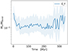 |
Fig. A.1. Ratio between the modidifed-Bondi accretion rate Ṁin and the classical Bondi rate in simulation qcrE_f. |
A.2. The derivative of fEdd
Here we compute the derivative of fEdd and find an approximate expression suitable for interpreting results shown in section 5.1. Starting from Eq. (A.6) and replacing a/J• = c/GM•2, the time derivative of fEdd reads
 (A.9)
(A.9)
where in the second row, we plugged in Eqs. (A.1, A.2), and (A.4) in place of Ṁα, Ṁ∙ and  and, for Eq. (A.4), we approximated all vectors as lying along the same direction. Eq. (A.9) can be simplified as follows. First, we note that
  , according to the definition of
  (Eq. A.5). In other words, the removal of mass and angular momentum from the disk due to the wind ejection does not affect the disk accretion rate. In addition,
  and
and  are both
  , being Mα ≪ M•. Similarly, noting that TBP in Eq. (A.3) doesn’t affect affect the spin modulus but only its direction, we can write
  since the specific angular momentum of gas orbiting at the ISCO is much smaller than the disk total specific angular momentum Jα/Mα. In this way, Eq. (A.9) reduces to
 (A.10)
Now, if we write  (see Section A.1) and
  (using Eq. 5), we obtain
 (A.11)
This equation points out that the leading terms driving the evolution of fEdd are the loss of mass due to accretion, here expressed in terms of Ṁw, and the replenishment of mass from resolved scales, represented by Ṁin. If we define the coefficients Cw = ηw−1 and Cin = (1 − 5⟨Λ⟩/7(Jα/Mα)) we get Eq. (17). For our choice of parameters, being vw/c = 0.01, we have that Cw = 0.1(η/0.1)−1 is of the same order of Cin, whose value is shown in Fig. A.2 for the three simulations qcrE.
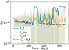 |
Fig. A.2. Coefficients Cin in qcrE simulations. The lines correspond to the median values over time bins of 5 Myr, while the shaded regions span from the 16th to the 84th percentiles over these bins. The coefficient Cw is also shown for the qcrE_f run. |
Appendix B: CGM energetic balance
In this section we discuss more in detail the energetic balance in the CGM, i.e. we compare the cooling luminosity of the gas and the energy flux of the outflow. The cooling luminosity is defined as  , where Λcool, i is the total cooling function of the i−th particle and the sum spans over the N gas particles in the radial bin [r − ΔR/2, r + ΔR/2), where we used ΔR = 1.5 kpc. We defined the energy flux of the outflow as
  , where vi, ui and vr, i are the i-th particle velocity, internal energy and radial velocity. In Fig. B.1 we show the time averages (over the same snapshots accounted in 5.2.4) of these quantities for the qcrE simulations.
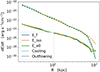 |
Fig. B.1. Time averages of the cooling luminosity (dashed) and outflow energy flux (solid) radial profiles for the qcrE simulations. Time averages are taken considering snapshots up to 180 Myr from t0. |
For each simulation, the location where the two energy rates become comparable roughly coincides with the maximum radius within which the CGM is affected by the outflow, as shown in the Fig. 14. While for anisotropic feedback (qcrE_f and qcrE_a0) this occurs at R ∼ 100 kpc, for isotropic feedback (qcrE_iso) the region impacted by the outflow extends beyond the radial range considered.
Appendix C: Wind particles
In this section we study the mass resolution of wind particles and the location where such particles are merged to nonwind particles for qcrE_f simulation. In Fig. C.1 we show the normalized histograms of the wind particles masses at four snapshots of qcrE_f: at one quarter, one half, three quarters and at the end of the simulation. The vertical cyan line shows the value of the nonwind particle mass resolution. According to this figure, wind particles throughout the simulation have masses orders of magnitude smaller than the initial ISM resolution, reason why we exclude the possibility that at the time of spawning these particles could result in a significant and instantaneous perturbation of the gas density surrounding the MBH. In addition, we considered the location where wind particles are merged into ISM particles. Figure C.2 shows the normalized histogram of the radii where such mergers occur throughout all qcrE_f simulation. It follows that wind particles capture is much more likely to occur within the first few hundreds pc from the MBH, but still takes place up to a distance of ∼10 kpc.
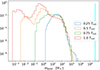 |
Fig. C.1. Normalized histograms of wind particles masses at four snapshots of qcrE_f simulation. The cyan line indicates the mass of nonwind particles at the beginning of the simulation. |
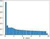 |
Fig. C.2. Normalized histogram of the radii where winds particles merge with ISM particles in qcrE_f simulation. |
All Tables
All Figures
|
Fig. 1. Luminosity angular pattern η(a)f(θ; a) for different spin values. |
| In the text | |
|
Fig. 2. Radiative efficiency (left y-axis) and the effective radiation semiopening angle (right y-axis) as a function of the spin parameter a. |
| In the text | |
|
Fig. 3. Schematic view of the outflow structure in a slice subtended by a solid angle ΔΩ and centered in a direction forming an angle θ with the MBH spin. This stratified structure comprises the AGN wind, the shocked wind (which extends up to a distance R(θ, t) from the MBH), the shocked ISM, and the unperturbed ISM. The illustration also shows the warped accretion disc that feeds the spinning MBH. |
| In the text | |
|
Fig. 4. Final snapshots of the propagation of an AGN wind-driven outflow for different spin values (increasing from left to right) and the two considered regimes (energy-driven in the top row and momentum-driven in the bottom one). Each panel illustrates the density, temperature, and pressure fields in units of the corresponding quantities of the assumed background medium as well as the wind mass fraction. In the energy-driven simulations, the outflow can be divided into four distinct sections: (1) the freely expanding wind, (2) the shocked wind, (3) the shocked ambient medium, and (4) the undisturbed ambient medium. In the momentum-driven simulations, radiative cooling makes the shocked wind layer cool and regions (2) and (3) are condensed into a thin shell. The wind tracer is injected together with the wind and is therefore only present in regions (1) and (2). The black lines correspond to the analytical location of the contact discontinuity between regions (2) and (3), as computed in Eqs. (11)–(13). In momentum-driven simulations, the cyan dashed lines indicate the effective aperture of the radiation as defined in Sect. 2.1. |
| In the text | |
|
Fig. 5. Density slices of three snapshots from simulation qcrC_f, with the disk face-on in the top panels and side-on in the bottom panels. The MBH location is marked by a black dot. |
| In the text | |
|
Fig. 6. Density slices of three snapshots from simulation qcrE_f, with the disk face-on in the top panels and side-on in the bottom panels. The MBH location is marked by a black dot. |
| In the text | |
|
Fig. 7. From left to right, edge-on maps of the gas density, the wind mass fraction, the internal energy, and the electron abundance fraction of simulation qcrE_f at t = 24 Myr. |
| In the text | |
|
Fig. 8. Evolution of the mass inflow rate Ṁin on the subgrid disk and the mass outflow rate Ṁw ejected in winds for the three qcrE simulations. The solid and dashed lines correspond to the median values of these quantities over time bins of 5 Myr, while the shaded regions span from the 16th to the 84th percentiles of Ṁin and Ṁw within the bins. |
| In the text | |
|
Fig. 9. Evolution of fEdd in qcrE and qcrC simulations. The lines correspond to the median values of fEdd over time bins of 5 Myr, while the shaded regions represent the fluctuations within the bins from the 16-th to 84-th percentiles. |
| In the text | |
|
Fig. 10. MBH spin and mass growth in qcrE and qcrC simulations. The red and blue bullet points mark the instants corresponding to the snapshots shown in Figures 5 and 6. |
| In the text | |
|
Fig. 11. Star formation rate in the nuclear region (left) and at galactic scale (right) for qcrE, qcrC, and qcrNoFb simulations. Here, t = 0 corresponds to the initial condition with the spinning gaseous halo in hydrostatic equilibrium and t0 = 150 Myr (when AGN feedback is turned on) is marked with a gray vertical line. |
| In the text | |
|
Fig. 12. Evolution of the central cavity size in qcrE, qcrC, and qcrNoFb simulations. |
| In the text | |
|
Fig. 13. Evolution of the outflow semiopening angle in qcrE, qcrC, and qcrNoFb simulations. |
| In the text | |
|
Fig. 14. Polar plots of the time averages of CGM temperature and entropy for qcrE simulations. Time averages are taken considering snapshots up to 180 Myr from t0. |
| In the text | |
|
Fig. 15. Time averages of the density radial profile of the CGM for the qcrE simulations. |
| In the text | |
|
Fig. A.1. Ratio between the modidifed-Bondi accretion rate Ṁin and the classical Bondi rate in simulation qcrE_f. |
| In the text | |
|
Fig. A.2. Coefficients Cin in qcrE simulations. The lines correspond to the median values over time bins of 5 Myr, while the shaded regions span from the 16th to the 84th percentiles over these bins. The coefficient Cw is also shown for the qcrE_f run. |
| In the text | |
|
Fig. B.1. Time averages of the cooling luminosity (dashed) and outflow energy flux (solid) radial profiles for the qcrE simulations. Time averages are taken considering snapshots up to 180 Myr from t0. |
| In the text | |
|
Fig. C.1. Normalized histograms of wind particles masses at four snapshots of qcrE_f simulation. The cyan line indicates the mass of nonwind particles at the beginning of the simulation. |
| In the text | |
|
Fig. C.2. Normalized histogram of the radii where winds particles merge with ISM particles in qcrE_f simulation. |
| In the text | |
Current usage metrics show cumulative count of Article Views (full-text article views including HTML views, PDF and ePub downloads, according to the available data) and Abstracts Views on Vision4Press platform.
Data correspond to usage on the plateform after 2015. The current usage metrics is available 48-96 hours after online publication and is updated daily on week days.
Initial download of the metrics may take a while.