| Issue |
A&A
Volume 685, May 2024
|
|
|---|---|---|
| Article Number | A92 | |
| Number of page(s) | 20 | |
| Section | Numerical methods and codes | |
| DOI | https://doi.org/10.1051/0004-6361/202348925 | |
| Published online | 14 May 2024 | |
Supermassive black hole spin evolution in cosmological simulations with OPENGADGET3★
1
Universitäts-Sternwarte, Fakultät für Physik, Ludwig-Maximilians-Universität München, Scheinerstr. 1, 81679 München, Germany
e-mail: This email address is being protected from spambots. You need JavaScript enabled to view it.
2
Astronomy Unit, Department of Physics, University of Trieste, via Tiepolo 11, 34131 Trieste, Italy
3
INAF – Osservatorio Astronomico di Trieste, via Tiepolo 11, 34131 Trieste, Italy
4
ICSC – Italian Research Center on High Performance Computing, Big Data and Quantum Computing, Bologna, Italy
5
Max-Planck-Institut für Astrophysik, Karl-Schwarzschild-Str. 1, 85741 Garching, Germany
Received:
12
December
2023
Accepted:
19
February
2024
Abstract
Context. The mass and spin of massive black holes (BHs) at the centre of galaxies evolve due to gas accretion and mergers with other BHs. Besides affecting the evolution of relativistic jets, for example, the BH spin determines the efficiency with which the BH radiates energy.
Aims. Using cosmological, hydrodynamical simulations, we investigate the evolution of the BH spin across cosmic time and its role in controlling the joint growth of supermassive BHs and their host galaxies.
Methods. We implemented a sub-resolution prescription that models the BH spin, accounting for both BH coalescence and misaligned accretion through a geometrically thin, optically thick disc. We investigated how BH spin evolves in two idealised setups, in zoomed-in simulations and in a cosmological volume. The latter simulation allowed us to retrieve statistically robust results for the evolution and distribution of BH spins as a function of BH properties.
Results. We find that BHs with MBH ≲ 2 × 10⁷ M⊙ grow through gas accretion, occurring mostly in a coherent fashion that favours spin-up. Above MBH ≳ 2 × 10⁷ M⊙, the gas angular momentum directions of subsequent accretion episodes are often uncorrelated with each other. The probability of counter-rotating accretion and hence spin-down increases with BH mass. In the latter mass regime, BH coalescence plays an important role. The spin magnitude displays a wide variety of histories, depending on the dynamical state of the gas feeding the BH and the relative contribution of mergers and gas accretion. As a result of their combined effect, we observe a broad range of values of the spin magnitude at the high-mass end. Reorientation of the BH spin direction occurs on short timescales (≲ 10 Myr) only during highly accreting phases (ƒEdd ≳ 0.1). Our predictions for the distributions of BH spin and spin-dependent radiative efficiency as a function of BH mass are in very good agreement with observations.
Key words: accretion, accretion disks / black hole physics / methods: numerical / galaxies: nuclei
Movie associated to Fig. 7 is available at https://www.aanda.org
© The Authors 2024
 Open Access article, published by EDP Sciences, under the terms of the Creative Commons Attribution License (https://creativecommons.org/licenses/by/4.0), which permits unrestricted use, distribution, and reproduction in any medium, provided the original work is properly cited.
This article is published in open access under the Subscribe to Open model. This email address is being protected from spambots. You need JavaScript enabled to view it. to support open access publication.
1 Introduction
Supermassive black holes (BHs; 106 ≲ MBH/ M⊙ ≲ 1010) at the centre of massive galaxies are observed as active galactic nuclei (AGN) if they accrete material from and release energy in their proximity. This process, dubbed AGN feedback, is able to significantly affect the surroundings of the BHs and it is thought to play a significant role in the evolution of massive galaxies (e.g. Benson et al. 2003; Di Matteo et al. 2005). Feedback has been broadly categorised in two modes, depending on the main channel of energy release (Churazov et al. 2005; Sijacki et al. 2007; Fabian 2012). In the so-called quasar mode, operating close to the Eddington limit, most of the energy is released in the form of radiation and winds (Silk & Rees 1998; Fabian 1999; Harrison et al. 2018). This mode is prevalent at earlier epochs (e.g. Croton et al. 2006). A second mode occurs at a highly sub-Eddington rate, when energy is channelled mostly into powerful relativistic jets (McNamara & Nulsen 2007, 2012; Cattaneo et al. 2009). This mode is often referred to as maintenance or radio mode. However, jets can also be efficient in super-Eddington accretion discs, which are found to become geometrically thick and able to confine the jet (Sądowski et al. 2014; Sądowski & Narayan 2015; Massonneau et al. 2023b; Lowell et al. 2024).
It has been advocated that rotating BHs have a fundamental role in the formation of jets (Davis & Tchekhovskoy 2020) and related feedback (McNamara & Nulsen 2012). The spin JBH of a BH with mass MBH can range from zero to the maximal value  . Thus, a BH is characterised by the dimensionless spin parameter a = JBH/Jmax. A maximally spinning 109 M⊙ BH can potentially provide ~1062 erg of rotational energy (McNamara & Nulsen 2012) that could be injected into the surroundings and offset cooling, once a mechanism to extract this energy is in action. Theoretically, a viable mechanism has been suggested by Blandford & Znajek (1977; see also Lasota et al. 2014). This process requires poloidal magnetic fields floated to an accretion flow, surrounding a rotating BH. The accreting matter drags the poloidal field into the BH ergosphere, where the BH rotation twists the field lines, generates a toroidal component of the field, and exerts an effective pressure that accelerates the plasma (see e.g. Tchekhovskoy 2015). Thus, the power of the jet is affected by the BH spin magnitude and the magnetic field flux threading the BH event horizon. The latter can be maximised in the so-called magnetically arrested disc state. In this configuration, magnetic flux is accumulated near the event horizon until it becomes dynamically relevant. In this state, the ratio between the jet power and accretion power (i.e. η = Pjet/(Ṁc2)) can be larger than one (Tchekhovskoy et al. 2011; McKinney et al. 2012; Narayan et al. 2022; Ricarte et al. 2023; Lowell et al. 2024). This is possible by extracting rotational energy from the BH. Launching powerful jets requires the presence of an accretion flow that acts as an float for the magnetic field and drags it inwards. If a jet is created, it is possible to tap into the rotational energy of the BH. Conversely, it is possible to power an AGN by accretion alone (without extracting spin energy), but in this case the maximum power output can only reach a few tens of percent of the accretion power.
Observationally, a connection between the BH spin and the jet power has been proposed to explain the observed radio-loudness (radio-to-optical flux density ratio, Sikora et al. 2007) in samples of AGN (e.g. Sikora et al. 2007; Martínez-Sansigre & Rawlings 2011). Ghisellini et al. (2010) found that the power of the most powerful jets in their sample of blazars (see Giommi et al. 2012, for a definition) can exceed the luminosity of the accretion disc by a factor of approximately ten. They argued that extraction of rotational energy may provide the additional power required. They also argued that if this is the case, the observed correlation between Pjet and accretion disc luminosity may arise from a link between the accretion and rotational energy extraction processes (as discussed above). The results published so far by the Event Horizon Telescope (EHT) collaboration have also favoured the extraction of rotational energy as a mechanism to efficiently produce jets (Event Horizon Telescope Collaboration 2021, 2022). Furthermore, although instrumental capabilities have prevented a conclusive confirmation so far, future polarimetry measurements with EHT could provide more direct observational support for this process (Chael et al. 2023).
The direction of the BH spin also plays a key role in jet formation. Spinning BHs create an outward Poynting flux in the direction of the BH spin, through the Blandford–Znajek mechanism (Hawley & Krolik 2006; Nakamura et al. 2008). Several observations of nearby clusters exhibit the presence of multiple pairs of jet-inflated cavities that have distinct angular orientations relative to the central galaxy (e.g. Forman et al. 2007; David et al. 2009; Sanders et al. 2009; Fabian et al. 2011; Hlavacek-Larrondo et al. 2015). This suggests multiple generations of jets propagating along different directions. The observations may be interpreted as spin re-orientation, provided that processes close to the BH manage to modify the BH spin and thus the launching direction of the jet (e.g. accretion proceeding on different planes across subsequent events). A few numerical works have demonstrated that it is possible to recover the observed morphologies by assuming a re-orienting jet (Cielo et al. 2018; Horton et al. 2020; Lalakos et al. 2022).
Black hole spins evolve across cosmic time due to accretion and mergers. Observational estimates of the BH spin parameter are therefore crucial to gain insight into its evolution. Several methods have been adopted in the literature to infer the BH spin of AGN (e.g. X-ray reflection methods or thermal continuum fitting, see Reynolds 2021, for a review). Most of the measurements published to date have been based on X-ray reflection spectroscopy based on Fe K lines. Recent works have developed a new class of high-density disc models (Jiang et al. 2019, 2022), which have been used to estimate the spin in low-mass BHs by modelling the X-ray relativistic reflection continuum (Mallick et al. 2022). The observed jet powers can also be used to determine the spin (Daly 2009, 2011, 2019, 2021). This method is particularly useful because it can be applied to large samples of AGN exhibiting jets. Lastly, interferometric observations with the EHT might provide constraints on the spin of M87* from the circularity of the shadow (Broderick et al. 2022), from the phase-twisting of light propagating near the BH (Tamburini et al. 2020), or from the linear polarisation pattern (Palumbo et al. 2020). The former method was only able to infer a clockwise rotation with the current observational capabilities (i.e. a spin vector pointing away from Earth). The latter provided an estimate of a = 0.90 ± 0.05 and an angle with respect to the line of sight i = 163° ± 2°.
From the theoretical standpoint, several analytical studies have been focussed on investigating the mechanism driving spin evolution that is likely linked to the coupling between the accretion disc and the BH spin (Bardeen 1970; Pringle 1981; Scheuer & Feiler 1996; Natarajan & Pringle 1998; Natarajan & Armitage 1999; King et al. 2005; Martin et al. 2007; Perego et al. 2009). If a geometrically thin, optically thick disc is misaligned with respect to the BH spin rotation axis, the innermost part aligns with the BH spin and is connected to the unperturbed outermost part through a smooth warp (Bardeen-Petterson effect). The flow through this region exerts a torque on the BH spin, modifying its direction. Recently, full general-relativistic magneto-hydrodynamic simulations performed by Liska et al. (2019) were able to reproduce this effect in magnetised thin discs.
Further works have focussed on building upon the analytical theory to understand the evolution of BH spin as a response of accretion and mergers, as well as the relative contribution between the two channels. A number of works adopted a semi-analytical treatment in a hierarchical cosmological context, with various recipes for the drivers of gas accretion and its effect on spin evolution (Volonteri et al. 2005; Berti & Volonteri 2008; Lagos et al. 2009; Fanidakis et al. 2011; Sesana et al. 2014; Griffin et al. 2019; Izquierdo-Villalba et al. 2020). Other studies focussed on simulating evolutionary histories of BHs under the assumption of a fixed fuelling angular momentum distribution and analysed how it affects the distribution of BH spins (Volonteri et al. 2007; King et al. 2008; Dotti et al. 2013; Zhang & Lu 2019). Going a step further, some works developed models suitable to be used on the fly in hydrodynamical simulations (Maio et al. 2013; Fiacconi et al. 2018), to study isolated systems at a high resolution. The model by Fiacconi et al. (2018) was also coupled to novel feedback recipes for winds (Cenci et al. 2020; Sala et al. 2021) and jets (Talbot et al. 2021). Recently, using the same model, Bollati et al. (2023) studied the dynamics of massive BH binaries in the presence of spin-dependent radiative feedback, whereas Talbot et al. (2023) focussed on the effect of jets in gas-rich galaxy mergers. While all of the above-mentioned works assumed a thin accretion disc, Huško et al. (2022) developed a spin evolution model that assumes a thick disc and applied it to study jet feedback in galaxy clusters. Dubois et al. (2014a) made a further step forward and developed a model suited to cosmological, hydrodynamical simulations, built upon the work of Volonteri et al. (2007) and King et al. (2005, 2008). The model was used to perform zoom-in simulations (Dubois et al. 2014a) and later updated to include jets, with a BH spin-dependent direction and power (Beckmann et al. 2019; Dubois et al. 2021; Dong-Páez et al. 2023; Massonneau et al. 2023a; Koudmani et al. 2023; Peirani et al. 2024).
Comparatively fewer works have been dedicated to the study of spin evolution in a cosmological box and have used a large statistical sample of BHs. Dubois et al. (2014b) ran their spin evolution model, although only in post-processing, on the output of the HORIZON-AGN simulation. Bustamante & Springel (2019) performed a set of simulations of a cosmological volume, evolving the spin on the fly with a similar model, although with a few differences at the sub-resolution level with respect to our implementation (see Sects. 2.2 and 6). In this work, we focus on studying supermassive BH spin evolution with a sub-resolution model that follows the latter two works. Our aim is to take full advantage from the statistically significant simulated population of BHs in a cosmological box. Using information provided by cosmological, hydrodynamical simulations, we aim to analyse in detail the coupled evolution of the spin direction and magnitude, the effect of the dynamical state of the gas fuelling the BHs, and the impact of mergers.
This paper is organised as follows. Section 2 describes the theoretical basis of our model and its implementation. Section 3 presents the suite of simulations we used to test our model and statistically study BH spins. Section 4 presents our simulation results, whereas in Sect. 5 we discuss their implications. In Sect. 6, we compare our work with previous studies in the literature. In Sect. 7, we summarise and conclude.
2 The model
In this section, we present our sub-resolution model for spin evolution due to gas accretion onto BHs and mergers and its coupling to the resolved scales. We implement our model in the TREEPM code OPENGADGET3 (see Groth et al. 2023), descendant of a non-public evolution of the GADGET-3 code (originally from Springel 2005). The code features a modern smoothed particle hydrodynamics (SPH) description (Beck et al. 2016) and adopts a bias-corrected, sixth-order Wendland kernel (Dehnen & Aly 2012) with 295 neighbours.
2.1 BH treatment
Our sub-resolution model is built within the broader BH physics module for cosmological simulations originally described in Springel et al. (2005b), with modifications as in Hirschmann et al. (2014) and Steinborn et al. (2015). Each BH in our simulations is treated as a collisionless sink particle, coupled to other particles only by gravity. We associate an SPH kernel to every BH (with smoothing length hBH) in a similar fashion as for the gas particles, with the same number of neighbours. The gravitational force on the BH is softened using a Plummer-equivalent softening length ɛBH. Its value is specific for each simulation and stated in the corresponding subsections. To select haloes where to seed new BH particles, we apply a FoF (Friends-of-Friends) algorithm to the stellar particles alone. In this way, we identify stellar bulges. We adopt a linking length of l = 0.05 and require that a halo has a stellar mass corresponding to M*,seed to host a new BH seed. We also demand that the halo has a stellar over dark matter (DM) mass fraction f* > 0.05 and a gas over stellar mass fraction fgas > 0.1, to ensure that the identified stellar bodies are newly forming galaxies and not tidally stripped stellar remains. The seed is created at the position of the star particle with the largest binding energy within the group, with an initial mass MBH,seed. The values of MBH,seed and M*,seed for each simulation are stated in the corresponding subsections. Alternatively, BHs with specific properties can be inserted in the initial conditions (ICs) to study a specific configuration of an idealised system (Sects. 3.1 and 3.2).
We do not apply any pinning of the BHs to the position of the potential minimum within hBH. Besides, we do not apply any drag force from the continuous gas accretion onto the BH and keep position and velocity of the central BH when BHs merge. We allow BHs to merge if the following criteria are met: (i) their relative velocity is smaller than 0.5cs, where cs is the sound speed of the gas, averaged in a kernel-weighted fashion; (ii) their distance is smaller than five times ɛBH; (iii) the binary binding energy is smaller than  (see Hirschmann et al. 2014, for further details).
Besides mergers, BHs also increase their mass1 by accreting gas. The mass inflow rate onto the BH is computed using the Bondi–Hoyle–Lyttleton prescription (hereafter Bondi; Hoyle & Lyttleton 1939; Bondi & Hoyle 1944; Bondi 1952):
 (1)
(1)
where ρ is the gas density, v is the velocity of the BH with respect to the gas and G is the gravitational constant. We compute the properties marked with 〈⋅〉 as a kernel-weighted average over the BH neighbouring particles. We also enforce a maximum radius on hBH for the computation, racc = 100 kpc. The dimensionless parameter αacc is often adopted to account for the detailed turbulent structure of the interstellar medium (ISM) in the vicinity of the BH (e.g. Springel et al. 2005a; Booth & Schaye 2009; but see e.g. Valentini et al. 2020), typically unresolved in cosmological simulations because of the limited spatial resolution (~kpc). Following Steinborn et al. (2015), we compute two different Bondi rates (motivated by e.g. Gaspari et al. 2013, as thoroughly discussed in Steinborn et al. 2015) using αacc,hot = 10 and αacc,cold = 100 (unless stated otherwise) for the hot and cold gas phases2 respectively. We assume that the accretion rate onto the BH is given by
 (2)
(2)
where ṀEdd = 4πGMBHmp/(σTϵrc) is the Eddington (1916) accretion rate, mp the proton mass, σT the Thomson cross section, c the speed of light, and ϵr the radiative efficiency. The latter depends on the BH dimensionless spin parameter in our simulations, as explained in Sect. 2.2.1.
2.2 Spin evolution algorithm
Our model is designed for simulations whose spatial resolution ranges from few tens of parsecs to a few kiloparsecs (see Sect. 3), several orders of magnitudes larger than the physical size of an accretion disc around a BH (< 1pc, Frank et al. 2002). In the approach often adopted in cosmological simulations, an accretion disc is not included in the modelling (e.g. Springel et al. 2005b; Booth & Schaye 2009). In our implementation, we introduce a sub-grid accretion disc as an intermediate step in the mass transfer between the resolved scales and the BH. We then assume that the mass transfer rate from the resolved scales onto the accretion disc is equal to the mass rate from the accretion disc onto the BH. The mass rate is defined by Eqs. (1) and (2). We also assume that the gas maintains the angular momentum direction it has at the resolved scales. The inclusion of an accretion disc is necessary to model the physical effects that modify the spin due to gas accretion, as explained in the following.
2.2.1 Accretion disc and spin evolution
We define the BH angular momentum vector JBH as
 (3)
(3)
where jBH is the unit vector encoding its direction and JBH is its magnitude. We define 0 ≤ a ≤ 1. In what follows, a negative sign encodes counter-rotating conditions on a BH with spin parameter a. JBH evolves because of its interaction with the distribution of matter in a surrounding accretion disc, whose angular momentum is misaligned with respect to JBH. Our model assumes an optically thick, geometrically thin Shakura & Sunyaev (1973) accretion disc.
If we start from a completely flat disc surrounding a spinning BH, Lense–Thirring precession forces the fluid elements close to the BH to precess and induces them to rotate in the BH equatorial plane. If viscosity is sufficiently high, the shear stresses propagate the perturbation diffusively until a warped steady state of the disc is reached (Bardeen & Petterson 1975; Martin et al. 2007). The largest deviation from a flat profile – that is, disc annuli where the gas angular momentum is misaligned with respect to both the unperturbed outer region of the disc and the BH spin – occurs at the warp radius. The latter is defined as the radius Rw at which the Lense-Thirring precession timescale  (Wilkins 1972) is equal to the warp propagation timescale
  (Pringle 1981; Perego et al. 2009). The vertical shear viscosity ν2 governs the propagation of vertical perturbations (e.g. Volonteri et al. 2007; Perego et al. 2009; Dotti et al. 2013; Dubois et al. 2014b). Following Dubois et al. (2014b), we computed
 (4)
(4)
where MBH,8= MBH/(108 M⊙), ϵr,01 = ϵr/0.1 and we define the Eddington ratio fEdd = ṀBH/ṀEdd. The radial shear viscosity ν1 is responsible for the radial inward drift of gas across the disc. We also assume that the viscosity α-parameter (Shakura & Sunyaev 1973) is  , following King et al. (2005), and
  , following Ogilvie (1999), leading to a fiducial value for the ratio ν2/ν1 = 85.
The flow of matter through the warp is responsible to exert a torque that modifies only the direction of the BH spin. Indeed, matter flowing from the unperturbed outermost region to the aligned innermost region through the warp changes its angular momentum direction, therefore forcing the BH spin orientation to change and ensure conservation of the total angular momentum (King et al. 2005; Dotti et al. 2013). Since the torque acting to modify the direction of the BH spin is produced by matter flowing through the warped region at Rw, we adopt the same assumption as Volonteri et al. (2007) and Dubois et al. (2014b) and define Jd = Jdjd as the angular momentum of the disc within Rw. King et al. (2005) showed that starting from a configuration where JBH and Jd are initially misaligned, the torque resulting from the warped configuration always leads the BH spin to align with the total angular momentum Jtot of the system disc+BH
 (5)
(5)
Moreover, the torque acts dissipatively on the disc, whose angular momentum ends up either aligned or counter-aligned with the BH spin, depending on the ratio between the angular momentum magnitudes. Namely, the counter-aligned configuration is possible if and only if
 (6)
(6)
where θBH−d is the angle subtended by the initial angular momentum directions jBH and jd (i.e. cos θBH−d = jBH ⋅ jd). Only the (counter-) aligned innermost (i.e. within Rw) region can effectively transfer its angular momentum to the BH, once the matter enclosed within this region is eventually accreted (Volonteri et al. 2007). Therefore, Rw is also the relevant radial scale to estimate the variation of the BH spin magnitude as a result of the accretion of this innermost part. Since the radial shear viscosity ν1 is responsible for the inward drift of matter across the disc, the region within Rw is accreted on a timescale  (King et al. 2005; Perego et al. 2009; Dubois et al. 2014b). We follow Dubois et al. (2014b) and compute
 (7)
(7)
We note that ν1 ≪ v2 and the warp propagation timescale tw is thus much shorter than the radial drift timescale  . As a consequence, the timescale on which the warp forms is much shorter than that over which the spin magnitude and direction change. We then estimate the mass enclosed within the warped region Md as
 (8)
(8)
where ṀBH is given by Eq. (2). When Md is accreted onto the BH, the BH spin magnitude a changes due to the accretion of its ISCO angular momentum, according to the expression derived in Bardeen (1970)
![Mathematical equation: ${a_{\rm{f}}} = {1 \over 3}{{r_{{\rm{isco}}}^{1/2}} \over {{M_{{\rm{ratio}}}}}}\left[ {4 - {{\left( {3{{{r_{{\rm{isco}}}}} \over {M_{{\rm{ratio}}}^2}} - 2} \right)}^{1/2}}} \right],$](/articles/aa/full_html/2024/05/aa48925-23/aa48925-23-eq17.png) (9)
(9)
where
 (10)
(10)
and, normalising to the gravitational radius Rg = RBH/2 = GMBH/c2,
![Mathematical equation: ${r_{{\rm{isco}}}} = {R_{{\rm{isco}}}}/{R_{\rm{g}}} = 3 + {Z_2} \pm {\left[ {\left( {3 - {Z_1}} \right)\left( {3 + {Z_1} + 2{Z_2}} \right)} \right]^{1/2}},$](/articles/aa/full_html/2024/05/aa48925-23/aa48925-23-eq19.png) (11)
(11)
where the positive (negative) sign is for counter(co)-rotating orbits. Z1 and Z2 are functions of the BH dimensionless spin parameter only:
![Mathematical equation: ${{Z_1} = 1 + {{\left( {1 - {a^2}} \right)}^{1/3}}\left[ {{{(1 + a)}^{1/3}} + {{(1 - a)}^{1/3}}} \right],}$](/articles/aa/full_html/2024/05/aa48925-23/aa48925-23-eq20.png) (12)
(12)
 (13)
(13)
The quantity Risco ranges from 1 to 9 Rg, for co- and counter-rotating orbits on a maximally spinning BH respectively, as illustrated in the bottom panel of Fig. 1. Physical sizes are therefore between ~5 × 10⁻⁶MBH,8 pc and ~5 × 10⁻⁵MBH,8 pc. The mass accreted is also corrected for the radiated energy, where
 (14)
(14)
The top panel of Fig. 1 shows the value of ϵr as a function of a.
Finally, as mentioned before, we estimate the angular momentum Jd of the accreted disc region that determines the spin variation in magnitude and direction (and is also used to evaluate condition (6)) as
 (15)
(15)
where  is the keplerian angular frequency. While Risco ~ 1 − 9Rg, the warped region is at hundreds of gravitational radii (see Eq. (4)), thus a few orders of magnitude larger. Therefore, the BH spin direction changes on a shorter timescale than its magnitude (Scheuer & Feiler 1996; Perego et al. 2009; Dotti et al. 2013).
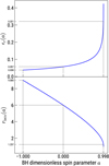 |
Fig. 1 Radiative efficiency – Eq. (14) – (top panel) and radius of the innermost stable circular orbit – Eq. (11) – (bottom panel), as a function of the BH dimensionless spin parameter. Some reference values of these quantities are also highlighted: a = −1, for a counter-rotating orbit around a maximally spinning BH; a = 0, for a non-spinning BH; a = 0.998, for the maximum spin allowed in our simulations. |
2.2.2 BH spin update iteration
The algorithm that we adopt to update BH mass and spin in our simulations models the above-mentioned processes, and makes sure that the BH mass grows consistently with the rate given by Eq. (2). Following Dubois et al. (2014b), BH mass and spin are updated in iterations (hereafter accretion episodes) composed of the following steps:
- 1.
We assume that an accretion disc forms around the BH, characterised by the accretion rate given by Eq. (2). We further assume that the initial angular momentum direction of the disc jd is set by the resolved scales of the simulation, parallel to the direction of the angular momentum of the gas within the BH kernel jg:
 (16)
(16)where
 (17)
(17)LBH,kernel is computed considering only the cold gas particles – the component that is able to settle into an accretion disc. w is the dimensionless SPH kernel function. This is the initial misaligned configuration illustrated on the left in Fig. 2.
- 2.
We compute Rw using Eq. (4). This defines the region of the disc (marked in blue in Fig. 2) that exerts the alignment torque on the BH spin and whose gas is eventually accreted by the end of the accretion episode.
- 3.
We compute Md and Jd, using Eqs. (8) and (15) respectively. This defines the total angular momentum of the accretion episode Jtot = JBH + Jd = JBH + Jdjd (black solid vector in Fig. 2). We note that we are assuming that the warped distribution that defines the innermost aligned region of the disc (central panel in Fig. 2) develops on a timescale shorter than those over which the BH spin direction and magnitude change, as explained in Sect. 2.2.1.
- 4.
We establish whether the innermost part of the disc is co- or counter-rotating using Eq. (6), by computing
 (18)
(18)
 (19)
(19)In case of counter-rotating conditions, risco and ϵr are computed with a negative sign in front of a.
- 5.
The final BH spin direction changes as a result of the alignment torque and ends up parallel to the total angular momentum (vector scheme on the right in Fig. 2), i.e.
 .
. - 6.
The disc within Rw is consumed and the BH spin magnitude changes according to Eq. (9) (right panel in Fig. 2), with Md computed in step 3. Counter-alignment is taken into consideration as described in step 4. We also cap the spin parameter to 0.998, which is the maximum spin allowed if photon trapping is assumed (Thorne 1974). The BH mass is increased by ∆MBH = Md(1 − ϵr).
We stress that it is possible to update the BH magnitude and direction separately because the latter changes over a shorter timescale than the former, meaning that first the BH spin aligns with the total angular momentum, then the magnitude changes because of accretion at the ISCO (for a detailed discussion on the impact of relevant timescales, see Perego et al. 2009; Dotti et al. 2013). Moreover, Eq. (9) does not depend on the direction, because it models angular momentum accretion from the innermost disc region, that is (counter-)aligned with the equatorial plane of the spinning BH due to the Bardeen–Petterson effect.
We also note that the mass per accretion episode Md might be smaller or larger than the amount of mass required to be accreted during the simulation timestep ∆t. Therefore, we follow Bustamante & Springel (2019) and adopt the following strategy:
if Md < ṀBH∆t, multiple accretion episodes occur over one BH simulation timestep ∆t. We allow for timestep sub-cycles indexed with a counter variable, therefore executing N = ṀBH∆t/Md accretion episodes. All the sub-cycles share the same accretion rate, computed at the beginning of the timestep. At the end of each sub-cycle (i.e. accretion episode) we update BH spin and mass.
if Md > ṀBH∆t, we adopt the same strategy extending the counter across multiple timesteps. The code executes N = Md/(ṀBH∆t) timesteps, then the accretion episode ends and the BH mass and spin are updated using averages for the accretion rate necessary in Eqs. (4), (8), and (18), namely
 (20)
(20)
Figure 3 illustrates how the final value of a after a single accretion episode depends on Mratio, for a few example values of initial a, assuming no misalignment is present. We note that the plotted lines do not correspond to evolutionary tracks of the BH in our simulations, the latter ones being defined instead by a succession of multiple accretion episodes, each one characterised by different initial directions and different values for Mratio and risco. The solid and dotted lines correspond to counter-rotating events. Figure 3 shows that a single counter-rotating accretion episode on a maximally spinning BH (solid line) would be able to spin it down to a = 0, if the accreted mass per episode were ≃25% of the BH initial mass. It would require an accreted mass of -2 times the BH mass to spin it up to a = 1, in a direction opposite to the initial one. Similarly, a counter-rotating accretion episode on a BH with a = 0.5 (dotted line) would require ≃ 0.1 MBH and 1.75 MBH to achieve the same results, respectively. An accretion episode on a non-spinning BH (dashed line) needs to be 1.5MBH to spin it up to its maximal value, whereas it needs to be equal to ≃MBH to obtain the same result on a BH with a = 0.5 in co-rotating conditions (dash-dotted line).
 |
Fig. 2 Schematic of the steps that compose a single accretion episode. The vector schemes in the upper part of the figure represent the initial and final configurations of the angular momenta, in a case similar to the one shown in Fig. lb by King et al. (2005). Left: an accretion disc settles around the BH, in a misaligned configuration. Centre: a warp develops, and the innermost part is forced to rotate in the BH equatorial plane and either co- or counter-align. Right: the BH spin changes in magnitude when gas is accreted at the innermost stable orbit. |
2.2.3 Self-gravity regime
Depending on the physical conditions, parts of the accretion disc could become unstable because of their own self-gravity (Dotti et al. 2013). This occurs at radii that are beyond
 (21)
(21)
The mass stable against fragmentation (see Dotti et al. 2013) is then
 (22)
(22)
Under this condition, only the region of the disc within Rsg can be accreted. Therefore, if Rsg < Rw we set Md = Msg and substitute Rw with Rsg in Eqs. (15) and (18). In this case,
 (23)
(23)
Whenever a BH is seeded, its spin is set to zero. As soon as ṀBH > 0, a disc is initialised with an angular momentum equal to
 (24)
(24)
since we assume that only the portion of the disc that is stable against fragmentation can eventually accrete on the BH. The rest of the algorithm proceeds as before. Msg and Rsg are computed using Eqs. (21) and (22) respectively.
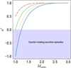 |
Fig. 3 Final BH spin dimensionless parameter after a single accretion episode as a function of Mratio as defined in Eq. (10). The solid, dotted, dashed and dot-dashed lines represent af for the initial spin values −1, −0.5, 0, and 0.5 respectively. The solid and dotted lines represent the event of an accretion episode in which the accretion disc is counter-rotating with respect to the BH. |
2.3 BH mergers
We implement a prescription to account for spin evolution in the case of BH mergers. In what follows, we adopt the same strategy as Dubois et al. (2014b) and Bustamante & Springel (2019). We use equations retrieved in a full general-relativistic framework by Rezzolla et al. (2008a) to compute the final spin after a merger event. Following their notation, we define a = ajBH. Once two BHs characterised by masses M1, M2 and spins a1, a2 have been selected to merge according to the criteria described in Sect. 2.1, the final spin vector of the remnant BH af is given by
 (25)
(25)
where q = M2/M1, with M1 ≥ M2. In this formula, M1 and M2 are the BH physical masses. ℓ = ℓ′/(M1 M2) where ℓ′ is the binary orbital angular momentum that cannot be radiated away in gravitational waves before coalescence. The magnitude of ℓ is provided by Rezzolla et al. (2008a) and reads
 (26)
(26)
Here, cos ϕ = a ⋅ ℓ/(aℓ) depicts the angle subtended by the spin vector of BH with ℓ, µ = q/(1 + q)2. s4 = −0.129, s5 = −0.384, t0 = −2.686, t2 = −3.454, t3 = 2.353 are the parameters of the fit to their numerical results. We assume that ℓ is parallel to the binary angular momentum L = L1 + L2 (Rezzolla et al. 2008a). Li=1,2 is the angular momentum vector of BH i with respect to the binary centre of mass (CM), computed as Li = Mi(ri − rCM) × (υ − υCM). The values for the radii ri and velocities υi are retrieved when the BHs are selected to merge.
2.4 AGN feedback
Our AGN feedback model assumes that a fraction ϵf of the radiated energy is coupled to the local ISM (refer to Sect. 3 for values), as often adopted in cosmological simulations (see e.g. Springel et al. 2005a; Booth & Schaye 2009). The total rate of coupled energy is thus:
 (27)
(27)
where ϵf is the coupling efficiency of the feedback energy to the surrounding ISM. An amount of energy  is distributed among the particles surrounding each BH in a weighted fashion, using the SPH kernel. Moreover, we follow Hirschmann et al. (2014) and implement a transition from quasar- to maintenance-mode feedback by assuming a coupling efficiency ϵf larger by a factor of four when fEdd < 0.01. In our model, the radiative efficiency ϵr depends on a through Eq. (14). This is at variance with other implementations where ϵr is either kept fixed (e.g. Springel et al. 2005b; Booth & Schaye 2009; Hirschmann et al. 2014) or depends on the accretion rate and BH mass using a phenomenological prescription (e.g. Steinborn et al. 2015).
3 The suite of simulations
In the following sections, we present our suite of simulations. The simulations are carried out with an advanced formulation of SPH (Beck et al. 2016), including a low-viscosity scheme (Dolag et al. 2005; Donnert et al. 2013) and isotropic thermal conduction (Dolag et al. 2004). The code also features metallicity-dependent radiative cooling, using the procedure described in Wiersma et al. (2009), and accounts for the presence of a uniform, time-dependent ionising background (Haardt & Madau 2001). We adopt the model by Springel & Hernquist (2003) to include a stochastic treatment of star formation and to describe the multiphase ISM, so that each gas particle (with hydrogen number density above a threshold nH = 0.5 cm−3) is made up of a cold, star-forming phase in pressure equilibrium with a hot phase. A detailed chemical evolution model (Tornatore et al. 2007) allows us to account for the metal enrichment of the ISM by ageing and exploding stars. We assume the lifetime function by Padovani & Matteucci (1993), and stellar yields for supernovae type Ia by Thielemann et al. (2003), supernovae type II by Nomoto et al. (2013) and asymptotic giant branch stars by Karakas & Lattanzio (2007). Each star particle represents a simple stellar population described by a Chabrier (2003) initial mass function.
We consider two idealised cases, a galaxy in isolation (Sect. 3.1) and a galaxy merger (Sect. 3.2), to test the model in a simple setup and study the evolution of the BH spin in a well-controlled environment. We also consider three setups in a full cosmological context (Sects. 3.3 and 3.4), which is key to capture the effects that the complex interplay between accretion and feedback can have on BH spin evolution. All the tests are performed including cooling, as well as star formation and evolution. The cosmological simulations include AGN and stellar feedback, whereas the idealised tests are performed with stellar feedback but no AGN feedback.
3.1 Idealised Milky Way galaxy
The first test we present is based upon the setup described in Steinwandel et al. (2019) aimed at modelling a Milky Way-like galaxy with total halo mass of M200 = 1012 M⊙ in isolation with a BH at the potential minimum. M200 is the mass enclosed within the spherical region whose average density is 200 times the critical density of the Universe. We defer the reader to their paper for the detailed procedure used to generate the ICs.
Table 1 summarises the initial properties of the central BH in our tests. We consider a fiducial case (IdealGal-fid), initialised with Mbh,0 = 5 × 10⁶ M⊙, a0 = 0.5, θz,0 = 170° and fEdd = 1. θz is the angle subtended by the BH spin and the z-axis. We perform further tests modifying one parameter at a time with respect to the fiducial run. Each simulation is labelled according to the value of the modified parameter, as in Table 1. Each test assumes a fixed Eddington fraction ƒEdd for the duration of the simulation.
The resolution is the same for all the tests. Masses of DM, gas and star particles are: mDM = 9.6 × 10⁵ M⊙, mg=m* = 4.8 × 10⁴ M⊙, respectively; the softening lengths are: εDM = 218 pc and εg = ε* = εBH = 50 pc.
Parameter summary for the idealised tests.
 |
Fig. 4 Gas density map of the ICs for the galaxy merger. The black arrows trace the local gas projected velocity field, while the white arrows indicate the initial direction of the CM of each galaxy. The arrows are scaled arbitrarily for visualisation purposes. |
3.2 Idealised galaxy merger
The second set of ICs describes a galaxy merger with a mass ratio of 1:1, initialised following the procedure described in Karademir et al. (2019).
The setup consists of two identical Milky Way-like galaxies, each with mass M200 = 1.89 × 10¹² M⊙. Each of them is embedded in a DM halo and has a spherical stellar bulge component, as well as an exponential stellar and gas discs. The initial separation of their CMs is 80 kpc and they rotate one around the other in the same direction in which they complete their revolution. The angle between the line connecting the two galaxy centres and their initial velocity vectors is equal to 40°. Figure 4 shows the setup. The BHs are initialised with a = 0 and MBH = 2 × 10s M⊙.
In this setup, mDM = 3.22 × 10⁶ M⊙, mg = m* = 1.86 × 10⁶ M⊙, εDM = 83 pc and εg = ε* = εBH = 20 pc.
3.3 Zoom-in simulations
We perform our zoom-in simulations starting from ICs generated with the procedure described in Bonafede et al. (2011). We consider two halos: a region with target mass M200 ≃ 1012 h−1 M⊙, dubbed ASIN; a region with target mass M200 ≃ 1013 h−1 M⊙, dubbed DFROGIN. They are selected from a parent DM-only simulation of a periodic box with side length Lbox = 1 h−1 cGpc and resolution mDM = 109 h−1 M⊙. The final resolution is quoted in Table 2, together with the properties and parameters of each simulation. This set of simulations adopts a flat ΛCDM cosmo-logical model, with a matter density parameter Ωm = 0.24, a baryon density parameter Ωb = 0.04 and h = 0.72. The initial power spectrum follows n = 0.96 and is normalised to σ8 = 0.8.
3.4 Cosmological box
We carry out a simulation starting from the ICs of the cosmological volume with Lbox = 48 h−1 cMpc (hereafter Box4) of the Magneticum3 simulations suite. Such a simulation, that contains ~103 BHs at redshift z = 0, allows us to analyse the properties of a statistically significant BH population, rather than focussing only on the specific behaviour of a few BHs.
Table 2 summarises the properties and parameters of the simulation. It assumes a flat ΛCDM model, with Ωm = 0.272, Ωb = 0.0456 and h = 0.704, n = 0.963 and σ8 = 0.809.
4 Results
4.1 Idealised Milky Way galaxy
Figure 5 presents the BH spin evolution in the tests listed in Table 1. Top left panel shows the time evolution of θz, the angle between jBH and the unit vector indicating the positive z-axis jz. The isolated galaxy is initialised with the angular momentum of the accreting gas along jz (i.e. θz=π refers to the BH spin direction being anti-parallel to the galaxy angular momentum, while θz = 0 refers to complete alignment). According to condition (6), counter-rotating accretion requires both jd • jBH > π/2 and Jd < 2JBH· In IdealGal-fid, IdealGal-120, IdealGal-5e5, IdealGal-5e7 and IdealGal-0.3 both conditions are satisfied at the beginning. However, the accreting gas in the BH surroundings keeps the same direction across the entire simulation (i.e. jg remains constant). As a result, the initial sub-grid disc direction jd for every accretion episode is also constant (Eq. (16), jg = jd). Therefore, each of them induces the BH spin to tilt towards the angular momentum direction of the large-scale external reservoir. We note that also Jd/JBH is approximately constant in these runs (a and ϵr vary slightly, but Jd/JBH depends weakly on them, see Eq. (19)). Whether or not condition (6) is verified in these tests depends only on jd•jBH (actually only on jBH, since jd is constant). Each vertical dotted line marks the first instant in which accretion becomes co-rotating (from counter-rotating; i.e. condition (6) is no longer verified after this instant). In IdealGal-fid the BH spin completes its alignment with the external reservoir in ~2 Myr. If we keep the same Eddington ratio but change the BH mass (IdealGal-5e5 and IdealGal-5e7, respectively), alignment takes the same time. On the other hand, alignment takes longer (~5 Myr) to complete with the same mass but a lower Eddington ratio (IdealGal-0.3). At fixed BH mass and Eddington ratio (IdealGal-fid, -120, and -30), the alignment timescale depends weakly on the initial misalignment angle. A smaller θZ,0 leads to a faster alignment.
The bottom left panel of Fig. 5 illustrates the time evolution of the BH spin parameter a. Since IdealGal-fld, IdealGal-120, IdealGal-5e5, IdealGal-5e7 and IdealGal-0.3 start with counter-rotating accretion conditions, a decreases. At t≃1 Myr co-rotating conditions take over and a starts increasing. The turnaround point occurs in correspondence of the dotted line, after which condition (6) is no longer verified. In IdealGal-30, a monotonically increases as condition (6) is not verified from the very beginning.
The top right panel of Fig. 5 shows θz as a function of the ratio MBH/MBH,0. At fixed θz,0 (IdealGal-fid, -5e5, -5e7, and -0.3), the same ratio of accreted mass over BH mass (MBH ~ 5% MBH,0) is needed for complete alignment to occur, regardless of other parameters. The actual time it takes to align depends on how fast the BH accretion proceeds. BHs whose spin starts with smaller θZ,0 (IdealGal-120 and -30) require less time.
The bottom right panel of Fig. 5 presents a as a function of the ratio MBH/MBH,0· Similarly to the bottom left panel, the turnaround point occurs in correspondence of the dotted line, when accretion switches from counter- to co-rotating. This plot further shows that it occurs at about the same value of MBH/MBH,0 at fixed θZ,0. Finally, for smaller θZ,0 a smaller ratio is required to reach the turnaround point.
The behaviour of both θz and a as a function of MBH/MBH,0 is similar for simulations assuming the same θZ,0 because ƒEdd is fixed. Indeed, the BH grows according to the following differential equation
 (28)
(28)
where τS = σTc/(4πGmp) ~ 4.5 × 10⁸ yr is the Salpeter time. As a result,
 (29)
(29)
Therefore, the evolution of θz and a as a function of time is different depending on ƒEdd (compare IdealGal-fid and IdealGal-0.3). On the other hand, the curves overlap if we consider MBH/MBH,0 as the independent variable (and they are independent of MBH,0 – see IdealGal-fid, IdealGal-5e5, IdealGal-5e7).
Parameter summary of the cosmological simulations.
 |
Fig. 5 Spin alignment process in the idealised Milky Way galaxy. Top panels: angle subtended by the BH angular momentum and the z-axis θr. Bottom panels: BH spin parameter a. Quantities are plotted as a function of time (left panels) and of the ratio between accreted and initial BH mass MBH/MBH,0 (right). Each line represents one simulation of the set summarised in Table 1. Dotted lines represent the instant after which condition (6) is no longer satisfied. |
4.2 Idealised galaxy merger
Figure 6 presents the evolution of the spins of the two BHs (one identified with the solid blue lines and the other with the dashed orange lines) in the idealised merger simulation. The left panel shows the evolution of quantities for the entire simulated times-pan, whereas the right panel shows a 2 Myr window, centred on the merger instant, marked in both panels by the vertical grey dotted line.
The first row from the top of Fig. 6 shows the separation distance between the BHs. The galaxies undergo three pericen-tre passages before the BHs merge (left panel), at ~336.15 Myr (right panel).
The second row of Fig. 6 follows the evolution of the spin parameter a. The left panel shows that both BHs follow an identical path from zero spin to maximal within 50 Myr (the two galaxies of the pair are identical). They are kept at maximal spin by accretion occurring consistently on the same plane, until the third pericentre passage. At this stage accretion becomes less coherent – that is, the direction of the local angular momentum has larger variability – and a decreases slightly due to counter-rotating accretion conditions. In the right panel, second row, just before the merger instant we identify two progenitors with a ~ 0.9. The final remnant has a ~ 0.9.
The third row of Fig. 6 shows the evolution of MBH. On the left, we see that the mass increases steadily and identically for the two BHs. The right panel allows us to identify two equal-mass progenitors with MBH = 1.2 × 10⁶ M⊙ merging into a remnant of MBH = 2.4 × 10⁶ M⊙.
Rows four to six of Fig. 6 show the three components of the BH spin direction. In the left panel we see that the two BHs consistently accrete from the same plane, hence their spins are kept very well aligned with the angular momentum direction of the host galaxies, which is along jz. The pericentre passages create some disturbance in the gas close to the BH, temporarily inducing the BH spin to tilt. This effect is more prominent close to the merger. In the right panel, we see that the BH spin components immediately before the merger are close to jz, although with some disturbances induced by the local environment. Furthermore, the spin of the remnant is also aligned with jz.
Figure 7 represents visually the process just described, using a volume rendering of the gas density in the simulation, for two simulation snapshots. The field of view depicted in the figure spans a width of 55 kpc and a height of 31 kpc, as measured along a plane that intersects the centre of the rendering volume, offering a perspective view of the merging galaxies. The arrows represent the instantaneous directions of the BH spins. The top panel of Fig. 7 corresponds to the instant marked by the green dash-dotted line in the right panel of Fig. 6, showing the pre-merger configuration. The bottom panel of Fig. 7 corresponds to the time marked by the purple dashed line, displaying the post-merger configuration.
The idealised galaxy merger test enables a simplified computation of the expected BH spin of the merger remnant to validate the result obtained. The pre-merger configuration (as shown in the right panels of Fig. 6 and in the top panel of Fig. 7) can be approximated to the idealised configuration of an equal-mass BH binary with aligned spins treated in Rezzolla et al. (2008b). In this configuration, the final spin magnitude af depends only on the initial spin magnitudes a1 and a2 (and the final direction is equal to the initial one). Two BHs with a ~ 0.9 and spins in the same direction are indeed expected to end up in a merger remnant with a ~ 0.9 and spin along the original, common rotation axis, as observed in our test.
 |
Fig. 6 Time evolution of a few properties of the two BHs (each of them is depicted by either blue solid or orange dotted lines) in the idealised galaxy merger simulation. From top to bottom: separation distance between the two BHs; BH dimensionless spin parameter; BH mass; x,y, z component of the unit vector of the BH angular momentum. Left panel: entire simulated timespan. Right panel: timespan of 2 Myr, centred on the time of the merger (grey, dotted vertical line). The vertical green dash-dotted and purple dashed lines mark the instants in time illustrated in the top and bottom panel of Fig. 7, respectively. |
4.3 Zoom-in simulations
Figure 8 presents projected gas density maps at z = 0 of ASIN (top) and DFROGIN (bottom). The white dots mark the positions of the BHs in the simulation. In what follows, we consider only the BHs that lie within a spherical region of radius 5R200 at z = 0, centred on the target halo of interest of the zoom-in region (i.e. the most massive one at z = 0). R200 is the radius of the spherical volume, centred on the subhalo, whose average density is 200 times the critical density of the Universe. The region is marked by the white circle in Fig. 8. The main purpose of this selection is to exclude BHs that are close the border of the high-resolution region.
Figure 9 shows the BH sample at z = 0 in ASIN (diamonds) and DFROGIN (stars) in the BH mass-stellar mass (MBH − M*) plane. The BHs are selected according to the criterion explained above; the sample is composed by four BHs in ASIN with 106.5 ≲ MBH/M⊙ ≲ 108 and 21 BHs in DFROGIN, with 106 ≲ MBH/M⊙ ≲ 109. Each BH is associated to a subhalo identified with the sub-structure finder algorithm SUBFIND (Springel et al. 2001; Dolag et al. 2009) based on particle ID matching. Whenever more than one BH is associated to the same subhalo, the closest to the subhalo centre is chosen. M* is the stellar mass as computed by SUBFIND. The dashed line shows the experimental fit by McConnell & Ma (2013), while crosses with associated uncertainties show observations from Kormendy & Ho (2013).
Figure 10 presents the spin parameters of the BHs in the simulated regions as a function of MBH at z = 0, with the same symbols used in Fig. 9. We compare our simulation output to the available observations that provide estimates of a and BH mass, with associated uncertainties. We include the collection by Reynolds (2021), with updates by Bambi et al. (2021) as described in Sisk-Reynés et al. 2022, as well as the low-mass sample by Mallick et al. (2022). We also include the spin estimate by Walton et al. (2021). In particular, we include the result by Sisk-Reynés et al. (2022), who provide a well-defined constraint of the spin of a ~3 × 10⁹ M⊙ BH, the most massive for which such a measure has been obtained to date. We observe a range of BH masses (106 ≲ MBH/M⊙ ≲ 5 × 10⁷) where BH spins tend to be larger than a ~ 0.70, in both the simulated regions. Several of them are maximally spinning. For masses above 5 × 10⁷ M⊙, there are no maximally spinning BHs, whereas the most massive BH in each region systematically has a lower spin, a ≃ 0.25 in ASIN and a ≃ 0.1 in DFROGIN.
Figure 11 shows the time evolution of a few BH properties predicted by the sub-resolution model. We restrict our analysis to the most massive BH of the sample in DFROGIN, and focus on the relationship between BH spin and gas accretion as they evolve with time. The evolutionary tracks of the other BHs in the sample display features which are similar to those of our reference, most massive BH as for the interplay between the BH spin and the fuelling gas. The upper axis of Fig. 11 marks the time since the Big Bang, while the lower axis shows the redshift z. Across the panels, the vertical dashed lines mark the occurrence of mergers.
The top panel of Fig. 11 shows the z-components of jBH (black, solid line) and jg (orange, dashed line). Before 1.7 Gyr, jg varies gradually with time, with a clear, average trend and limited scatter. From ≃l.7 to ≃2.6 Gyr a trend in jg is still present but the scatter increases, jBH follows the average evolution of jg. From ≃2.6 to ≃6 Gyr, jg exhibits drastic and sudden changes, whereas jBH remains stable with minimal variations. After ≃6 Gyr, jBH often undergoes abrupt variations due to the erratic behaviour of jg.
The second row of Fig. 11 shows cos θBH–d (black solid line), the left-hand-side term of Eq. (6), as a function of time. The orange dashed line shows −Jd/(2JBH), the right-hand side of Eq. (6). Before ≃1.7 Gyr each accretion episode is characterised by consistently small misalignment. Between ≃l.7 and ≃2.6 Gyr several accretion episodes display θBH–d close to π/2. After ≃2.6 Gyr accretion episodes are mostly misaligned. This panel also allows us to easily identify counter-rotating accretion episodes, when cos(θBH–d ) < −Jd/(2JBH) (e.g. around 2.2 Gyr and 4.5 Gyr).
The third row of Fig. 11 shows Jd/2JBH, the ratio between the accretion disc and the BH angular momentum per accretion episode. This quantity controls how much a single accretion episode is able to modify the direction of the BH spin and ultimately determines to which degree the BH spin is able to follow the variations of jg. Being the BH spin direction  after an accretion episode parallel to then
  (i.e. the direction change is negligible; Sect. 2.2.2). Conversely, if Jd ⪢ JBH, then
  (i.e. jBH aligns with the direction imparted by jd and hence jg). In an intermediate configuration jBH only partially aligns with jd. The latter situation is expected to occur before ≃6 Gyr, when Jd/JBH ≲ 0.1. However, at t ≳ 6 Gyr Jd/JBH sometimes approaches 1; as a result, jBH exhibits larger variations as a response to large changes in jg. Although here we inspect the evolution of Jd/JBH and θBH–d for one BH as an example, we properly quantify how the change jBH depends on these two quantities by analysing accretion episodes statistically in the cosmological box (Sect. 4.4).
The fourth row of Fig. 11 shows the BH dimensionless spin parameter a. Its evolution is characterised by a maximally spinning phase until t ≃1.95 Gyr (z ≳ 3.3). The largest spin-downs occur because of mergers, although we also observe counter-rotating phases that decrease the spin due to gas accretion (e.g. at t ≃ 2.2 and ≃2.35 Gyr, as well as around 4.5 Gyr).
The fifth row of Fig. 11 plots the radiative efficiency, which depends on a (see Eq. (14)). The dash-dotted, dashed and dotted lines mark the values of efficiency for a = 0.998, 0 and for a counter-rotating episode on a BH with a = 1, respectively. The maximally spinning period before z ~ 3.5 corresponds to a maximal efficiency of 0.32, whereas later times are characterised by a lower efficiency. Counter-rotating accretion conditions are clearly visible as a drastic decrease in efficiency, close to the minimum theoretical value marked by the dotted line.
The sixth row of Fig. 11 illustrates the Eddington ratio ƒEdd· Accretion is Eddington-limited soon after the BH is seeded (z ~ 4.9). ƒEdd is typically ≳ 10–1 until z ~ 2.6. Between 0.9 ≲ z ≲ 2.6, ƒEdd ⪡10–1 for most of the time. A few highly accreting (ƒEdd ≃ 10−1) episodes occur in proximity of the mergers at z ~ 0.9 and z ~ 0.7, and lead to significant reorientation of the BH spin (see first row of Fig. 11). After z ~ 0.7 ƒEdd is mostly ≲10−3. Comparing with the evolution of a (fourth row of Fig. 11), we observe that the largest ƒEdd, the largest is the change induced in a.
The last row of Fig. 11 plots MBH· The BH increases its mass by three orders of magnitude during the highly accreting phase at z ≳ 2.6. After z ~ 2.6, the BH gets more massive (by about one order of magnitude) mostly due to mergers.
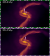 |
Fig. 7 3D perspective volumetric rendering of the gas density in the idealised galaxy merger simulation. The field of view depicted in the figure spans a width of 55 kpc and a height of 31 kpc, as measured along a plane that intersects the centre of the rendering volume. Top panel: last snapshot before the merger. Bottom panel: first snapshot after merger. The arrows mark the instantaneous direction of the BH spin vector. A movie is available online. |
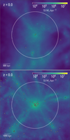 |
Fig. 8 Gas surface density maps at z = 0 for the ASIN (top) and DFROGIN (bottom) runs. The white circle indicates a spherical region of radius 5R200, centred on the target halo of the zoom-in region (i.e. the most massive at z = 0). The white dots mark the positions of the BHs in the simulation. |
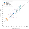 |
Fig. 9 MBH as a function of stellar mass M*, at z = 0. Diamonds and stars represent BHs in ASIN and DFROGIN, respectively. The dashed line shows the experimental fit by McConnell & Ma (2013), while crosses with associated uncertainties show data from Kormendy & Ho (2013). |
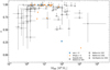 |
Fig. 10 BH spin parameters a of the selected BH sample in ASIN (diamonds) and DFROGIN (stars) as a function of MBH, at z = 0. The squares and pentagons show the collection of observational measurements of the BH spin parameter by Reynolds (2021; with updates from Bambi et al. 2021) and Mallick et al. (2022), respectively. The hexagon represents the spin estimate reported by Walton et al. (2021) and the diamond represents the measurement obtained by Sisk-Reynés et al. (2022). |
4.4 Cosmological box
For the analysis of BOX4 we consider all the BHs in the cosmological volume and we select them at z = 0. We associate each BH to a subhalo based on particle ΓD matching using SUBFIND and whenever more than one BH is associated to the same subhalo, the closest to the subhalo centre is chosen. The sample includes 1790 BHs, in a mass range between 6 × 10⁶ and 2 × 10¹⁰ M⊙.
Figure 12 frames the Box4 BH sample at z ~ 0 in the MBH − M*. plane. M* corresponds to the subhalo stellar mass as computed by SUBFIND. We compare our sample to observations by McConnell & Ma (2013) and Kormendy & Ho (2013; as in Fig. 9). Each point is colour-coded according to the number of mergers of the BH (including their progenitors). The number increases with increasing BH mass.
In Fig. 13, we show how BH spin parameters change as a function of MBH in Box4 (similar to Fig. 10). The simulated BHs are indicated by circles, and are colour-coded according to the number of mergers they have undergone. We compare our simulation output to the observational data by Reynolds (2021); Bambi et al. (2021); Walton et al. (2021); Sisk-Reynés et al. (2022); Mallick et al. (2022; as in Fig. 10). The BH sample is much more numerous than in the zoom-in regions and the mass range extends further on the high-end, up to 2 ~ 1010 M⊙. We identify three mass ranges in which we observe different distributions of α. Close to the seeding mass (~5.5 × 10⁵ M⊙), we can see a steep increase of a with MBH. We caution that the match with observations in this region is due to the choice of the seeding mass, which determines at which mass scale this regime of steep increase occurs. The BH population characterised by 106 ≲ MBH/ M⊙ ≲ 2 × 10⁷ shows a systematic tendency for highly spinning BHs (a ≳ 0.85), with most of them close to the maximal value. BHs with masses above 2 × 10⁷ M⊙ display a wider range of a, extending as low as a ~ 0.1. Moreover, we observe a sharp transition at MBH ~ 108 M⊙, associated clearly with the regime where mergers start to occur. This mass range also corresponds to the largest scatter in a. The robustness of this result is consolidated by the larger number of BHs probing this high-mass regime with respect to the zoom-in simulations. We also note that for MBH ≳ 5 × 10⁸ M⊙ there are no maximally spinning BHs.
Figure 14 shows the evolution of a of the five most massive BHs in the sample as a function of mass. The redshift is encoded in the colour gradient of each curve. The symbols mark the position of each BH in the plot at a few specific instants in time, corresponding to z = 0, 1, 2, 3, 4, colour-coded accordingly. As soon as the BHs are seeded, they undergo a phase of rapid increase of a, then they reach and maintain a maximally spinning state. We also notice that when MBH is between 106 and 2 × 10⁷ M⊙, BHs undergo short transitory periods of spin-down due to counter-rotating accretion or mergers. on the other hand, a reaches again the maximal state afterwards, highlighting that co-rotating accretion is dominant. After the BHs overcome the 2 × 10⁷ M⊙ mass scale, α exhibits a tendency to decrease. In addition, we observe large and sudden changes due to mergers (when also the mass increases significantly at the same time). A binary with BH spins oriented towards opposite directions results in a severe spin-down of the remnant compared to the state immediately before the merger. The wider distribution of a at the highest masses in Fig. 13 suggests that spin-down due to counter-rotating accretion and mergers occurs frequently.
In Fig. 15, we carry out a statistical analysis of a few key properties of the accretion episodes occurred in the Box4 run, to gain insight on the mechanisms with which gas accretion drives the trends observed in Figs. 13 and 14. For the analysis, the entire set of accretion episodes occurred during the simulation is considered (i.e. for every BH at every redshift). The top panel of Fig. 15 shows a 2D histogram where accretion episodes are binned according to their values of Jd/JBH and MBH. Each 2D bin is colour-coded by the number of accretion episodes in that bin. The dashed and dotted lines represent the dependence of Jd/JBH on mass from Eq. (18) (i.e.  for the self-gravitating case and
  for the standard case), assuming a = 0.998 and fEdd = 1. The distribution observed in Jd/JBH at fixed mass bin is due to different values of a and fĵdd· However, Jd/JBH depends weakly on the latter two quantities, while it depends on MBH quite strongly (see Eq. (19)). Above MBH ~ 108 M⊙ accretion occurs mostly in the self-gravitating regime (i.e. Rsg < Rw). The middle panel of Fig. 15 shows a 2D histogram where accretion episodes are binned according to their values of θBH–d and MBH. The solid white line indicates the median value of θBH–d per BH mass bin, whereas the shaded region represents the 25th and 75th percentile of the distribution of θBH–d in that BH mass bin. We observe that accretion episodes are characterised predominantly by small misalignment (75% of them has θBH–d ≲ 0.25 rad ~ 15°) below MBH ~ 108 M⊙. Above this mass threshold, the distribution broadens with increasing mass, showing that large misalignment is increasingly more probable. However, we caution that in this regime less accretion episodes occur, therefore the significance of this trend is limited by low-number statistics. We note that when Jd ⪡ JBH, the minimum angle required for an episode to satisfy condition (6) is θBH–d = π/2. The minimum angle is larger for larger Jd/JBH, whereas for Jd ≥ 2JBH accretion will be always co-rotating regardless the initial misalignment. Since a large misalignment is more probable at high BH masses (middle panel of Fig. 15) whereas Jd/JBH decreases with mass above MBH ~ 108 M⊙ (top panel of Fig. 15), counter-rotating accretion episodes are more likely. In the bottom panel of Fig. 15, we plot the fraction of accretion episodes that are counter-rotating with respect to the total number per BH mass bin. This fraction increases with increasing mass and it is as high as 0.5 for the highest mass bins. We also note that if the self-gravity prescription were not in place, Jd/JBH ≳ 1 above MBH ~ 108 M⊙, co-rotating conditions would be prevalent at all masses, and the gas accretion channel of spin evolution would have generally larger probability of increasing the spin.
It is now possible to assess the contribution of gas accretion to the trends discussed in Figs. 13 and 14 in light of the results shown in Fig. 15. Below MBH ~ 108 M⊙, most of the accretion episodes are co-rotating, therefore spin-up is favoured. Counter-rotating accretion episodes do occur, but the decrease in spin is transitory and co-rotating accretion leads the spin back to maximal. Conversely, above MBH ~ 108 M⊙ the probability of counter-rotating accretion (and hence spin-down) increases as a function of mass.
In Fig. 16, we quantify the direction variation imparted to the BH spin as a function of the properties of each accretion episode. The plot shows the angle ΔθBH between the direction of the BH spin before and after each accretion episode (i.e. ) in the Box4 run, as a function of Jd/JBH. The accretion episodes (circles) are colour-coded by θBH–d, the BH spin-disc misalignment at the beginning of the episode. The dashed lines indicate the analytical dependence computed using Eq. (5) and expressing
  as a function of Jd/JBH, at fixed θBH–d. If Jd ⪡ JBH then ΔθBH ~ 0, regardless θBH–d. If Jd ⪢ JBH, then ΔθBH ~ θBH–d. Increasing values of Jd/JBH induce larger alignment of jBH with jd per accretion episode. Fig. 16 also shows that, overall, Jd/JBH ≳ 1 is rare. Therefore complete alignment of jBH with jd (ΔθBH = θBH–d) never occurs in a single accretion episode and accretion episodes lead at most to partial alignment with the instantaneous direction of the accreting gas.
Figure 17 shows the radiative efficiency ϵr across the BH sample at z = 0, as a function of MBH. The trends shown in Fig. 13 are reflected in the distribution of ϵr. Indeed, each BH has its own value of ϵr at each instant, dependent on a (see Fig. 1). We observe predominantly high efficiency (~0.32) at intermediate BH masses (106 ≲ MBH/ M⊙ ≲ 2 × 10⁷). A lower efficiency value becomes more likely at higher masses (above 4 × 10⁷ M≲), whereas at the highest masses (above 5 × 10⁸ M≲) efficiencies have systematically lower values (~0.06–0.l). The radiative efficiency also depends on whether, at a given instant, accretion is proceeding in co- or counter-rotating accretion conditions. Points with ϵr below the dashed line correspond to BHs that are accreting in counter-rotating conditions. Indeed, the probability of having counter-rotating conditions increases with mass above 4 × 10⁷ M⊙ (bottom panel of Fig. 15). We also compare our simulated sample with a collection of radiative efficiency factors provided in Daly (2021). Since the simulation points refer to the sample at z = 0, we consider all the sources in the observational catalogue that have z < 0.24.
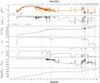 |
Fig. 11 Summary of properties related to the most massive BH in the DFROGIN run, as they evolve across time. From top to bottom: z-component of the BH spin direction jBH,z (black, solid line) and direction of the angular momentum of the gas in the BH kernel jg,z (orange, dashed line); cosine of the angle between the accretion disc and the BH spin at the beginning of each accretion episode cos θBH–d (i.e. left-hand side of Eq. (6), black solid line) and − Jd/(2JBH) (i.e. right-hand side of Eq. (6), orange dashed line); ratio of the magnitudes of the disc and BH angular momenta Jd/JBH; BH dimensionless spin parameter α; radiative efficiency of the accretion disc єr; Eddington ratio fEdd; BH mass MBH. |
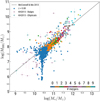 |
Fig. 12 MBH as a function of stellar mass M* for the Box4 run. Circles represent the simulated sample at z = 0, while the observational points are as in Fig. 9. The points are colour-coded according to the number of mergers BH have undergone. |
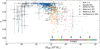 |
Fig. 13 Distribution of BH spin parameters as a function of the BH mass in Box4 (circles), at z = 0. The points are colour-coded according to the number of mergers BH have undergone. The squares and pentagons show the collection of observational measurements of the BH spin parameter by Reynolds (2021; with updates from Bambi et al. 2021) and Mallick et al. (2022), respectively. The hexagon represents the spin estimate reported by Walton et al. (2021) and the diamond represents the measurement obtained by Sisk-Reyn6s et al. (2022). |
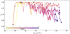 |
Fig. 14 BH dimensionless spin parameter a as a function of MBH, for the five most massive BHs at z = 0, for the Box4 run. Each line corresponds to one BH and is colour-coded by redshift. The symbols mark the position of each BH in the plot at a few specific instants in time, corresponding to z = 0, 1, 2, 3, 4, colour-coded accordingly. |
5 Discussion
5.1 Evolution of the BH spin direction
Our algorithm for spin evolution proceeds through accretion episodes that modify jBH as an effect of the external change in jg. As shown in Fig. 16, only if Jd ≫ JBH a single accretion episode is able to induce complete alignment with jd and therefore with jg. Conversely, if Jd ≪ JBH, then JBH is insensitive to external change. We observe that in our simulations accretion episodes are in general characterised by Jd/JBH ≲ 1 (Fig. 16), therefore accretion episodes induce only partial alignment of jBH with jd. Larger values of Jd/JBH reduce the misalignment between jBH and jg to a larger degree. The relation between jBH and jd (and hence jg) on timescales longer than a single accretion episode depends on Jd/JBH and on the variability of jg. For the reference BH considered in DFROGIN, the top panel of Fig. 11 shows that before t ~ 2.6 Gyr jg varies gradually with time, although with some variability on short (i.e. ≲1 Myr) timescales. On the other hand, jg changes erratically after t ~ 2.6 Gyr. In the former case jBH manages to follow the average evolution of jg, whereas the two directions are decoupled in the latter. The middle panel of Fig. 15 shows that statistically such large misalignment is more probable at the highest masses. Combined with low values of Jd/JBH, it results in counter-rotating accretion conditions to be more frequent with increasing mass (bottom panel of Fig. 15).
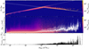 |
Fig. 15 Statistical analysis of a few key properties of the accretion episodes occurred in the Box4 run. The entire set of accretion episodes occurred during the simulation has been considered (i.e. for every BH and at every redshift). The top (middle) panel shows a 2D histogram of the values of Jd/JBH (θBH−d) as a function of mass. Each bin is colour-coded by the number of accretion episodes in that bin (Nbin), normalised to the total number of episodes per mass bin (Nmass bin). In the top panel, the dashed line pinpoints |


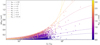 |
Fig. 16 BH spin direction variation per accretion episode (i.e. |


5.2 Evolution of the BH spin magnitude
The BH spin magnitude evolution via gas accretion is driven by the amount of accreted mass and by the radius of the ISCO (Eq. (9)). Therefore, it evolves more rapidly in high accretion rate phases. Furthermore, counter-rotating accreting gas is characterised by a larger ISCO (bottom panel of Fig. 1), thus a larger angular momentum per unit mass. The same amount of accreted mass induces a larger (negative) change in a than if it were accreted in co-rotating conditions. At fixed mass, if co-and counter-rotating episodes occurred in equal number, the net effect would actually be a decrease in a (Dotti et al. 2013). Whether there is a trend to increase or decrease the spin magnitude depends on the accretion rate and on how frequent co- or counter-rotating accretion is. Moreover, mergers also contribute to influence a. In Figs. 10 and 13, we analyse the trends of a with BH mass and observe that BHs with MBH ≲ 2 × 10⁷ M⊙ show systematic spin-up. This effect is attributed to the prevalence of co-rotating accretion conditions (bottom panel of Fig. 15). Mergers do not occur in this range of masses (see Fig. 13), hence the trend is exclusively due to gas accretion. For MBH ≳ 2 × 10⁷ M⊙, we observe a wide distribution of a, indicating that the behaviour strongly depends on the detailed history, and there is no systematic behaviour. In this mass regime, several elements contribute to the trend: i) the fraction of counter-rotating episodes increases with mass (bottom panel of Fig. 15) but it remains generally lower than 50%; ii) co-rotating conditions and hence spin-up still occur; iii) only the BHs in the highest mass bins (≳ 5 × 10⁹ M⊙) reach a fraction ≳ 0.5 and exhibit systematically low spins (a ≃ 0.2–0.3). We also note that above MBH ≳ 108 BHs undergo several mergers (Fig. 13) and Eddington ratios are generally highly sub-Eddington (e.g. second to last panel of Fig. 11). Therefore, mergers significantly contribute to the variation of the spin. Moreover, mergers with misaligned directions tend to significantly decrease a (e.g. fourth panel of Fig. 11). From Fig. 13, we infer that the widening of the distribution at the high masses is associated with the increasing importance of mergers and a more likely counter-rotating accretion.
In Fig. 13, we also note that BHs close to the seeding mass (MBH ≃ 5.5 × 10⁵ M⊙) are characterised by a steep increase of a with mass. The region in the a – MBH plane that these BHs occupy is mostly determined by MBH,seed. However, the initial value of a does not affect the following evolution, since any initial spin value is quickly evolved to maximal due to large accretion rates.
Overall, the trends in a as a function of MBH are consistent between the zoom-in simulations (Fig. 10) and the Box4 (Fig. 13), which even have different resolutions. The distribution of a is compatible with the observations within the uncertainties, across the entire mass range.
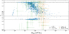 |
Fig. 17 Radiative efficiencies of the BH populations at redshift z = 0, as a function of mass, for the Box4 run. The triangles show the collection of empirical estimates of the radiative efficiency by Daly (2021). The dotted, dashed and dash-dotted lines mark the values of the efficiency corresponding to a = −1,0,0.998, respectively, for reference. The population in the bottom part of the figure represents the BH that are accreting in counter-rotating conditions. |
5.3 Radiative efficiency
The radiative efficiency plays an important role. First of all, it enters the computation of the Eddington accretion rate. Since the BH accretion rate cannot exceed this rate in our model, the efficiency directly affects the Eddington-limited growth phases. According to Eq. (29), the e-folding timescale
 (30)
(30)
depends on the efficiency. Eddington-limited co-rotating accretion on a maximally spinning BH (i.e. ϵr ~ 0.32) implies  Myr, whereas in counter-rotating conditions (ϵr ~ 0.038)
  Myr. A lower efficiency leads to a significantly faster BH growth. In our simulations, Eddington-limited phases are characterised by maximally spinning BHs and co-rotating accretion, thus growth proceeds with ϵr ~ 0.32 (see e.g. ϵr panel in Fig. 11).
The efficiency also controls the amount of feedback energy released to the surroundings, at a given ṀBH (see Eq. (27)). A lower efficiency implies less released energy and subsequent increased accretion. It also means a faster increase in MBH (because of the factor 1 − ϵr in Eq. (10)). This in turn boosts ṀBH (due to the ∝ MBH dependence in Eddington-limited phases or ∝  otherwise, see Eq. (1)), leading to stronger feedback outbursts that hinder accretion. In addition, since the Eddington accretion rate depends on the efficiency, the switch to maintenance mode feedback is also affected. Overall, the effects just discussed contribute in a non-trivial way to modify the evolutionary path of a BH through the feedback loop. Our simulations – where all these processes are self-consistently taken into account – show that BHs are on the observed correlation between BH mass and stellar mass (Figs. 12 and 9). While the detailed evolutionary path along the plane MBH − M*, changes, each BH is eventually able to approach the correlation, implying that the BHs still grow in an overall self-regulated scenario.
Figure 17 highlights that ϵr tends to decrease with increasing mass at the high-mass end. We also find that the distribution of our simulated sample is compatible with the distribution of empirical estimates by Daly (2021), within the uncertainties. We note that the empirical sample is obtained with a method that does not rely on a specific accretion disc model. Therefore, while our sample has an upper and lower limit for the efficiency determined by our theoretical assumption on the disc structure, the interpretation of the empirical estimates is not bound to such an assumption. On the other hand, assuming for the accretion disc a different model based, for instance, on a hot accretion flow (Yuan & Narayan 2014), would imply lower efficiencies than in the thin disc theory.
6 Comparison with previous works
Dubois et al. (2014b) and Bustamante & Springel (2019) perform a statistical study similar to ours. The former simulate a cosmological volume with size and resolution comparable to BOX4 and the latter a smaller box with higher resolution (Lbox = 25 h−1 cMpc and mDM = 8.4 × 10⁶ M⊙). Our spin evolution model follows Dubois et al. (2014b), although we track the spin on the fly whereas in their work the spin is tracked in post-processing. ϵr is assumed to be fixed to 0.1. They include a thermal feedback channel for fEdd > 0.01 and a bipolar outflow launched in the direction of the local gas otherwise, but both do not depend on a. Bustamante & Springel (2019) adopt an on-the-fly spin update algorithm similar to ours, with a variable ϵr affecting the thermal feedback mode. However, below a mass-dependent fEdd threshold, BHs inject purely kinetic energy, with a fixed efficiency and random direction, isotropic on average. Moreover, when the sub-grid accretion disc is affected by self-gravity the angular momentum direction of each accretion episode is extracted from a chosen angular distribution. In our implementation we assume it is fixed and equal to the gas angular momentum direction at all times. Interestingly, the trends we find in Fig. 13 are in agreement with both works, regardless of whether or not ϵr depends on a or whether the spin is evolved in post-processing rather than on the fly. This indicates that the variability of the radiative efficiency does not play a significant role in setting these trends. On the other hand, ϵr does affect AGN feedback and BH growth (Sect. 2.4). As a result, a different prescription for ϵr changes the detailed time evolution of BH mass and stellar mass, leading to a different path towards the MBH − M*, relation and more scatter around it (Bustamante & Springel 2019). Nonetheless, Fig. 12 shows that the self-regulated scenario is still present and eventually leads the BHs on the relation.
We find that the dynamical state of the feeding material, combined with the key parameter Jd/JBH, plays a significant role in the evolution of the BH spin due to gas accretion (Figs. 15 and 16). Dotti et al. (2013) conclude that when Jd/JBH ≪ 1 (as it occurs in our simulations, see Fig. 15), the feeding angular momentum distribution determines whether a increases or decreases. Our findings regarding the behaviour of the spin in response to the feeding conditions are in agreement with theirs, as well as with Dubois et al. (2014b) and Bustamante & Springel (2019). When the gas angular momentum direction varies slowly and its misalignment with respect to the BH spin is small (indicating a preferential direction), the BHs are maximally spinning. This generally occurs at MBH ≲ 108 M⊙ (see Figs. 11, 14, 15). Conversely, uncorrelated gas angular momentum directions lead to increasingly probable counter-rotating accretion and BH spin-down (bottom panel of Fig. 15, Sect. 4.4). We note that the large scatter in a at high masses (Fig. 13) is found also by Dubois et al. (2014a) and Bustamante & Springel (2019), despite the different prescriptions for AGN feedback. This might indicate that its effect is to generally induce loss of coherence in the angular momentum distribution (middle panel of Fig. 15), regardless of the specific channel.
In contrast to our model, Bustamante & Springel (2019) introduce stochasticity in jd (Eq. (16)) at the sub-resolution level, on top of the resolved variability in the simulation. Such a prescription can be thought as a way to account for turbulent structures in the ISM that are not resolved in cosmological simulations (see e.g. Murchikova et al. 2019; Ressler et al. 2020 for our Galactic centre). Bustamante & Springel (2019) assume that in the self-gravity regime jd is extracted from a distribution that ranges from random (isotropic) to concentrated around the preferential axis set by the local gas angular momentum (anisotropic). As a result, they observe a more pronounced decoupling between jd and jBH compared to us, in case of an isotropic distribution. On the other hand, they find the same widening of the distribution of a at high BH masses, regardless of the degree of anisotropy. Dubois et al. (2014a) also explore the effect of varying the distribution of jd at the sub-resolution level. However, they introduce stochasticity in all accretion regimes. They find that even a slight anisotropy leads to results that are very similar to the completely coherent case (i.e. when the gas preserves the angular momentum direction as measured by the simulation). Only if the gas angular momentum is randomly oriented at all masses, then BHs settle on a ~ 0.2–0.3 (King et al. 2008) and an increasing trend of spin with mass is found (Fanidakis et al. 2011; in those conditions the trend is produced by mergers, that tend to bring slowly spinning BHs to values around 0.7 for MBH ≳ 109 M⊙). One possibility to explain these results is that when gas accretion is sub-dominant, the trend is mainly driven by mergers. However, we observe that above MBH ≳ 108 M⊙ gas accretion does contribute to spin evolution, inducing both spin-up and spin-down (Fig. 14). The net effect depends crucially on the accretion rate, the BH environment and the level of anisotropy of the feeding gas. In our simulations such conditions arise naturally and we find that the level of anisotropy varies widely over time and across the BH population. In addition to gas accretion, mergers also contribute to modify the spin value (Fig. 13), but the relative contribution of gas accretion and mergers to spin evolution is different depending on the detailed cosmological history. We postpone a systematic study to a future work.
Finally, we note that we do not integrate the full differential equation that describes the precession and alignment process, due to the coupling between the gas distribution in the accretion disc and the BH spin (at variance with, e.g., Fiacconi et al. 2018). Rather, we assume that the process is discretised in accretion episodes and is globally taken into account, while the total angular momentum is conserved (Sect. 2.2), following King et al. (2005). Fiacconi et al. (2018) developed an algorithm that includes the full detailed treatment, although it requires high temporal and spatial resolution. In fact, timesteps as low as 10−3 Myr are required in some cases to meaningfully integrate the differential equation, which are prohibitive in a full cosmological context. Moreover, their model measures directly the inflow properties as resolved by the simulation at the sub-resolution boundary, rather than using an effective prescription such as the Bondi parametrisation. Therefore, it is suitable for high-resolution simulations (e.g. approximately a parsec scale). In contrast, we assume that the mass rate through the sub-resolution accretion disc is equal to the mass accretion rate onto the BH and it is identical to the Bondi accretion rate at all times. We further note that Fiacconi et al. (2018) model spin evolution only due to gas accretion, although mergers are expected to contribute to spin evolution for MBH ≳ 108 M⊙ (Fanidakis et al. 2011; Dubois et al. 2014a) and the low-redshift growth of massive BHs is dominated by mergers in several models (e.g. Weinberger et al. 2018; Pacucci & Loeb 2020). Although they do not produce a statistical sample of BHs, they perform a suite of simulations aimed at mimicking a range of realistic conditions. Despite the approach is different in a number of numerical aspects, the expected effect of the gas accretion channel on spin evolution is in line with ours: systematic spin-up for MBH ≲ 107 M⊙ and a wider distribution of a at higher masses.
7 Conclusions
We have implemented a sub-resolution model to track the evolution of BH spins due to gas accretion and mergers in large-scale cosmological simulations. The model assumes the presence ofa misaligned thin accretion disc perturbed by the metric of a spinning BH, which in turn experiences a torque that modifies its spin direction. The BH radiative efficiency and Eddington accretion rate are dependent on the BH spin and thus variable across cosmic time. Their impact on accretion and feedback is therefore captured self-consistently. We have designed a simulation suite featuring idealised, isolated systems (Sects. 4.1 and 4.2) to validate the model and cosmological setups (Sects. 4.3 and 4.4) to investigate statistical properties of the BH population. We summarise our findings as follows:
The ability of a single accretion episode to modify the BH spin depends on the amount of mass and angular momentum it carries with respect to the BH (Jd/JBH, Fig. 16). An accretion episode with larger Jd/JBH induces the BH spin direction jBH to tilt more towards the gas angular momentum direction jg;
The evolution of the direction and the magnitude of the spin are tightly coupled. When Jd/JBH ≲ 1 (Fig. 15), the feeding distribution of the gas angular momentum directions determines whether a preferably increases or decreases. If accretion occurs consistently along the same plane (e.g. Fig. 5), spin-up is expected. Conversely, if jg changes direction erratically, counter-rotating conditions and spin-down can occur (Figs. 11 and 15);
In a cosmological context, we identified two regimes, depending on the distribution of a with BH mass (Fig. 13). BHs with MBH ≲ 2 × 10⁷ M⊙ tend to be highly spinning (a ≳ 0.85). At the high-mass range (MBH ≳ 2 × 10⁷ M⊙), a exhibits a broad range of values;
We observed a wide variety of evolutionary histories for a (Fig. 14), depending on the dynamical state of the gas feeding the BH and the occurrence of coalescences. This indicates that the level of anisotropy of jg and the relative contribution of mergers and accretion varies across the BH population;
When jg exhibits some degree of coherence and varies slowly (generally at z ≳ 2 and MBH ≲ 2 × 10⁷ M⊙), jBH follows the average evolution of jg and small misalignment is observed (Fig. 15). At late times (z ≲ 2), jg shows large and abrupt changes, while jBH is stable over long periods (hundreds of millions of years, e.g. Fig. 11). Indeed, since Jd/JBH ≲ 1, accretion episodes are not able to modify significantly jBH. This frequently leads to large misalignment;
The tendency for maximal spin in the low-mass range is due to the accretion of co-rotating gas with small misalignment (Fig. 15). The wide range of values of a in the high-mass range is due to mergers and more isotropically distributed jg, and this results in a probability of counter-rotating accretion that increases with mass (Figs. 14 and 15). The distribution of jg arises self-consistently, as measured from the simulation;
Including a self-consistent ϵr has an important effect on determining the BH growth rate in the Eddington-limited phases. A higher efficiency during these phases implies a lower growth rate. Our statistical sample shows that BHs with MBH ≲ 4 × 10⁷ M⊙ always have efficiencies around 0.32, whereas the most massive BHs generally have lower efficiencies (Fig. 17);
Although the variable ϵr modifies the detailed path on the MBH − M*, plane, BHs eventually approach the observed correlation, indicating self-regulated growth;
The spin with which BHs are initialised is erased quickly after they are seeded. Massive BHs can retain some information on the dynamical state of the gas they recently accreted (Figs. 14 and 15).
We caution that so far we have coupled the spin evolution model to a single channel of energy injection, namely purely thermal, aimed at reproducing the radiative feedback. An additional mechanism, in which large-scale jets (tens to hundreds of kilo-parsecs) are the key actors, is thought to be specifically relevant at the high-mass end. We plan to include this feature in future works, by coupling the spin evolution model to a feedback channel from jets, which is dependent on the spin magnitude and direction.
Movies
Movie 1 associated with Fig. 7 Access Supplementary Material
Acknowledgements
We would like to thank the anonymous Referee for the valuable comments and insights, that helped to improve the content and the presentation of the manuscript. L.S. acknowledges support from ‘BiD4BEST’ – European Innovative Training Network (ITN) funded by the Marie Skłodowska-Curie Actions (860744) in Horizon 2020. M.V. is supported by the Fondazione ICSC, Spoke 3 Astrophysics and Cosmos Observations, National Recovery and Resilience Plan (PNRR) Project ID CN_00000013 “Italian Research Center on High-Performance Computing, Big Data and Quantum Computing” funded by MUR (Missione 4, Componente 2, Investimento 1.4: Potenziamento strutture di ricerca e creazione di campioni nazionali di R&S, M4C2-19) – Next Generation EU. M.V. also acknowledges partial financial support from the INFN Indark Grant. This work was supported by the Deutsche Forschungsgemeinschaft (DFG, German Research Foundation) under Germany’s Excellence Strategy -EXC-2094 – 390783311 and we are especially grateful for the support through the Computational Center for Particle and Astrophysics (C2PAP). Some of the analyses reported in this work have been performed using PYNBODY (Pontzen et al. 2013)
References
- Bambi, C., Brenneman, L. W., Dauser, T., et al. 2021, Space Sci. Rev., 217, 65 [CrossRef] [Google Scholar]
- Bardeen, J. M. 1970, Nature, 226, 64 [Google Scholar]
- Bardeen, J. M., & Petterson, J. A. 1975, ApJ, 195, L65 [Google Scholar]
- Beck, A. M., Murante, G., Arth, A., et al. 2016, MNRAS, 455, 2110 [Google Scholar]
- Beckmann, R. S., Dubois, Y., Guillard, P., et al. 2019, A&A, 631, A60 [EDP Sciences] [Google Scholar]
- Benson, A. J., Bower, R. G., Frenk, C. S., et al. 2003, ApJ, 599, 38 [NASA ADS] [CrossRef] [Google Scholar]
- Berti, E., & Volonteri, M. 2008, ApJ, 684, 822 [NASA ADS] [CrossRef] [Google Scholar]
- Blandford, R. D., & Znajek, R. L. 1977, MNRAS, 179, 433 [NASA ADS] [CrossRef] [Google Scholar]
- Bollati, F., Lupi, A., Dotti, M., & Haardt, F. 2023, MNRAS, 520, 3696 [NASA ADS] [CrossRef] [Google Scholar]
- Bonafede, A., Dolag, K., Stasyszyn, F., Murante, G., & Borgani, S. 2011, MNRAS, 418, 2234 [NASA ADS] [CrossRef] [Google Scholar]
- Bondi, H. 1952, MNRAS, 112, 195 [Google Scholar]
- Bondi, H., & Hoyle, F. 1944, MNRAS, 104, 273 [Google Scholar]
- Booth, C. M., & Schaye, J. 2009, MNRAS, 398, 53 [Google Scholar]
- Broderick, A. E., Tiede, P., Pesce, D. W., & Gold, R. 2022, ApJ, 927, 6 [NASA ADS] [CrossRef] [Google Scholar]
- Bustamante, S., & Springel, V. 2019, MNRAS, 490, 4133 [CrossRef] [Google Scholar]
- Cattaneo, A., Faber, S. M., Binney, J., et al. 2009, Nature, 460, 213 [NASA ADS] [CrossRef] [Google Scholar]
- Cenci, E., Sala, L., Lupi, A., Capelo, P. R., & Dotti, M. 2020, MNRAS, 500, 3719 [NASA ADS] [CrossRef] [Google Scholar]
- Chabrier, G. 2003, PASP, 115, 763 [Google Scholar]
- Chael, A., Lupsasca, A., Wong, G. N., & Quataert, E. 2023, ApJ, 958, 65 [NASA ADS] [CrossRef] [Google Scholar]
- Churazov, E., Sazonov, S., Sunyaev, R., et al. 2005, MNRAS, 363, L91 [NASA ADS] [Google Scholar]
- Cielo, S., Babul, A., Antonuccio-Delogu, V., Silk, J., & Volonteri, M. 2018, A&A, 617, A58 [CrossRef] [EDP Sciences] [Google Scholar]
- Croton, D. J., Springel, V., White, S. D. M., et al. 2006, MNRAS, 365, 11 [Google Scholar]
- Daly, R. A. 2009, ApJ, 696, L32 [NASA ADS] [CrossRef] [Google Scholar]
- Daly, R. A. 2011, MNRAS, 414, 1253 [NASA ADS] [CrossRef] [Google Scholar]
- Daly, R. A. 2019, ApJ, 886, 37 [CrossRef] [Google Scholar]
- Daly, R. A. 2021, MNRAS, 500, 215 [Google Scholar]
- David, L. P., Jones, C., Forman, W., et al. 2009, ApJ, 705, 624 [NASA ADS] [CrossRef] [Google Scholar]
- Davis, S. W., & Tchekhovskoy, A. 2020, ARA&A, 58, 407 [Google Scholar]
- Dehnen, W., & Aly, H. 2012, MNRAS, 425, 1068 [NASA ADS] [CrossRef] [Google Scholar]
- Di Matteo, T., Springel, V., & Hernquist, L. 2005, Nature, 433, 604 [NASA ADS] [CrossRef] [Google Scholar]
- Dolag, K., Jubelgas, M., Springel, V., Borgani, S., & Rasia, E. 2004, ApJ, 606, L97 [NASA ADS] [CrossRef] [Google Scholar]
- Dolag, K., Vazza, F., Brunetti, G., & Tormen, G. 2005, MNRAS, 364, 753 [NASA ADS] [CrossRef] [Google Scholar]
- Dolag, K., Borgani, S., Murante, G., & Springel, V. 2009, MNRAS, 399, 497 [Google Scholar]
- Dong-Páez, C. A., Volonteri, M., Beckmann, R. S., et al. 2023, A&A, 673, A120 [NASA ADS] [CrossRef] [EDP Sciences] [Google Scholar]
- Donnert, J., Dolag, K., Brunetti, G., & Cassano, R. 2013, MNRAS, 429, 3564 [Google Scholar]
- Dotti, M., Colpi, M., Pallini, S., Perego, A., & Volonteri, M. 2013, ApJ, 762, 68 [NASA ADS] [CrossRef] [Google Scholar]
- Dubois, Y., Volonteri, M., & Silk, J. 2014a, MNRAS, 440, 1590 [Google Scholar]
- Dubois, Y., Volonteri, M., Silk, J., Devriendt, J., & Slyz, A. 2014b, MNRAS, 440, 2333 [Google Scholar]
- Dubois, Y., Beckmann, R., Bournaud, F., et al. 2021, A&A, 651, A109 [NASA ADS] [CrossRef] [EDP Sciences] [Google Scholar]
- Eddington, A. S. 1916, MNRAS, 77, 16 [NASA ADS] [Google Scholar]
- Event Horizon Telescope Collaboration (Akiyama, K., et al.) 2021, ApJ, 910, L13 [Google Scholar]
- Event Horizon Telescope Collaboration (Akiyama, K., et al.) 2022, ApJ, 930, L17 [NASA ADS] [CrossRef] [Google Scholar]
- Fabian, A. C. 1999, MNRAS, 308, L39 [NASA ADS] [CrossRef] [Google Scholar]
- Fabian, A. C. 2012, ARA&A, 50, 455 [Google Scholar]
- Fabian, A. C., Sanders, J. S., Allen, S. W., et al. 2011, MNRAS, 418, 2154 [Google Scholar]
- Fanidakis, N., Baugh, C. M., Benson, A. J., et al. 2011, MNRAS, 410, 53 [NASA ADS] [CrossRef] [Google Scholar]
- Fiacconi, D., Sijacki, D., & Pringle, J. E. 2018, MNRAS, 477, 3807 [NASA ADS] [CrossRef] [Google Scholar]
- Forman, W., Jones, C., Churazov, E., et al. 2007, ApJ, 665, 1057 [NASA ADS] [CrossRef] [Google Scholar]
- Frank, J., King, A., & Raine, D. J. 2002, Accretion Power in Astrophysics: Third Edition (Cambridge, UK: Cambridge University) [Google Scholar]
- Gaspari, M., Ruszkowski, M., & Oh, S. P. 2013, MNRAS, 432, 3401 [NASA ADS] [CrossRef] [Google Scholar]
- Ghisellini, G., Tavecchio, F., Foschini, L., et al. 2010, MNRAS, 402, 497 [Google Scholar]
- Giommi, P., Padovani, P., Polenta, G., et al. 2012, MNRAS, 420, 2899 [NASA ADS] [CrossRef] [Google Scholar]
- Griffin, A. J., Lacey, C. G., Gonzalez-Perez, V., & Lagos, C. d. P. 2019, arXiv e-prints [arXiv: 1912.09490] [Google Scholar]
- Groth, F., Steinwandel, U. P., Valentini, M., & Dolag, K. 2023, MNRAS, 526, 616 [NASA ADS] [CrossRef] [Google Scholar]
- Haardt, F., & Madau, P. 2001, in Clusters of Galaxies and the High Redshift Universe Observed in X-rays, eds. D. M. Neumann, & J. T. V. Tran, 64 [Google Scholar]
- Harrison, C. M., Costa, T., Tadhunter, C. N., et al. 2018, Nat. Astron., 2, 198 [Google Scholar]
- Hawley, J. F., & Krolik, J. H. 2006, ApJ, 641, 103 [CrossRef] [Google Scholar]
- Hirschmann, M., Dolag, K., Saro, A., et al. 2014, MNRAS, 442, 2304 [Google Scholar]
- Hlavacek-Larrondo, J., McDonald, M., Benson, B. A., et al. 2015, ApJ, 805, 35 [NASA ADS] [CrossRef] [Google Scholar]
- Horton, M., Krause, M., & Hardcastle, M. 2020, MNRAS, 499, 5765 [NASA ADS] [CrossRef] [Google Scholar]
- Hoyle, F., & Lyttleton, R. A. 1939, Math. Proc. Camb. Phil. Soc., 35, 405 [NASA ADS] [CrossRef] [Google Scholar]
- Huško, F., Lacey, C. G., Schaye, J., Schaller, M., & Nobels, F. S. J. 2022, MNRAS, 516, 3750 [CrossRef] [Google Scholar]
- Izquierdo-Villalba, D., Bonoli, S., Dotti, M., et al. 2020, MNRAS, 495, 4681 [NASA ADS] [CrossRef] [Google Scholar]
- Jiang, J., Fabian, A. C., Dauser, T., et al. 2019, MNRAS, 489, 3436 [NASA ADS] [CrossRef] [Google Scholar]
- Jiang, J., Abdikamalov, A. B., Bambi, C., & Reynolds, C. S. 2022, MNRAS, 514, 3246 [NASA ADS] [CrossRef] [Google Scholar]
- Karademir, G. S., Remus, R.-S., Burkert, A., et al. 2019, MNRAS, 487, 318 [Google Scholar]
- Karakas, A., & Lattanzio, J. C. 2007, PASA, 24, 103 [NASA ADS] [CrossRef] [Google Scholar]
- King, A. R., Lubow, S. H., Ogilvie, G. I., & Pringle, J. E. 2005, MNRAS, 363, 49 [NASA ADS] [CrossRef] [Google Scholar]
- King, A. R., Pringle, J. E., & Hofmann, J. A. 2008, MNRAS, 385, 1621 [NASA ADS] [CrossRef] [Google Scholar]
- Kormendy, J., & Ho, L. C. 2013, ARA&A, 51, 511 [Google Scholar]
- Koudmani, S., Somerville, R. S., Sijacki, D., et al. 2023, MNRAS, submitted [arXiv:2312.08428] [Google Scholar]
- Lagos, C. D. P., Padilla, N. D., & Cora, S. A. 2009, MNRAS, 395, 625 [NASA ADS] [CrossRef] [Google Scholar]
- Lalakos, A., Gottlieb, O., Kaaz, N., et al. 2022, ApJ, 936, L5 [NASA ADS] [CrossRef] [Google Scholar]
- Lasota, J. P., Gourgoulhon, E., Abramowicz, M., Tchekhovskoy, A., & Narayan, R. 2014, Phys. Rev. D, 89, 024041 [NASA ADS] [CrossRef] [Google Scholar]
- Liska, M., Tchekhovskoy, A., Ingram, A., & van der Klis, M. 2019, MNRAS, 487, 550 [CrossRef] [Google Scholar]
- Lowell, B., Jacquemin-Ide, J., Tchekhovskoy, A., & Duncan, A. 2024, ApJ, 960, 82 [CrossRef] [Google Scholar]
- Maio, U., Dotti, M., Petkova, M., Perego, A., & Volonteri, M. 2013, ApJ, 767, 37 [NASA ADS] [CrossRef] [Google Scholar]
- Mallick, L., Fabian, A. C., García, J. A., et al. 2022, MNRAS, 513, 4361 [NASA ADS] [CrossRef] [Google Scholar]
- Martin, R. G., Pringle, J. E., & Tout, C. A. 2007, MNRAS, 381, 1617 [NASA ADS] [CrossRef] [Google Scholar]
- Martínez-Sansigre, A., & Rawlings, S. 2011, MNRAS, 414, 1937 [CrossRef] [Google Scholar]
- Massonneau, W., Dubois, Y., Volonteri, M., & Beckmann, R. S. 2023a, A&A, 669, A143 [NASA ADS] [CrossRef] [EDP Sciences] [Google Scholar]
- Massonneau, W., Volonteri, M., Dubois, Y., & Beckmann, R. S. 2023b, A&A, 670, A180 [NASA ADS] [CrossRef] [EDP Sciences] [Google Scholar]
- McConnell, N. J., & Ma, C.-P. 2013, ApJ, 764, 184 [Google Scholar]
- McKinney, J. C., Tchekhovskoy, A., & Blandford, R. D. 2012, MNRAS, 423, 3083 [Google Scholar]
- McNamara, B. R., & Nulsen, P. E. J. 2007, ARA&A, 45, 117 [NASA ADS] [CrossRef] [Google Scholar]
- McNamara, B. R., & Nulsen, P. E. J. 2012, New J. Phys., 14, 055023 [NASA ADS] [CrossRef] [Google Scholar]
- Murchikova, E. M., Phinney, E. S., Pancoast, A., & Blandford, R. D. 2019, Nature, 570, 83 [NASA ADS] [CrossRef] [Google Scholar]
- Nakamura, M., Tregillis, I. L., Li, H., & Li, S. 2008, ApJ, 686, 843 [NASA ADS] [CrossRef] [Google Scholar]
- Narayan, R., Chael, A., Chatterjee, K., Ricarte, A., & Curd, B. 2022, MNRAS, 511, 3795 [NASA ADS] [CrossRef] [Google Scholar]
- Natarajan, P., & Armitage, P. J. 1999, MNRAS, 309, 961 [NASA ADS] [CrossRef] [Google Scholar]
- Natarajan, P., & Pringle, J. E. 1998, ApJ, 506, L97 [NASA ADS] [CrossRef] [Google Scholar]
- Nomoto, K., Kobayashi, C., & Tominaga, N. 2013, ARA&A, 51, 457 [CrossRef] [Google Scholar]
- Ogilvie, G. I. 1999, MNRAS, 304, 557 [NASA ADS] [CrossRef] [Google Scholar]
- Pacucci, F., & Loeb, A. 2020, ApJ, 895, 95 [NASA ADS] [CrossRef] [Google Scholar]
- Padovani, P., & Matteucci, F. 1993, ApJ, 416, 26 [Google Scholar]
- Palumbo, D. C. M., Wong, G. N., & Prather, B. S. 2020, ApJ, 894, 156 [Google Scholar]
- Peirani, S., Suto, Y., Beckmann, R. S., et al. 2024, A&A, in press, https://doi.org/10.1051/0004-6361/202349101 [Google Scholar]
- Perego, A., Dotti, M., Colpi, M., & Volonteri, M. 2009, MNRAS, 399, 2249 [NASA ADS] [CrossRef] [Google Scholar]
- Pontzen, A., Roškar, R., Stinson, G., & Woods, R. 2013, Astrophysics Source Code Library, [record ascl:1305.002] [Google Scholar]
- Pringle, J. E. 1981, ARA&A, 19, 137 [NASA ADS] [CrossRef] [Google Scholar]
- Ressler, S. M., White, C. J., Quataert, E., & Stone, J. M. 2020, ApJ, 896, L6 [NASA ADS] [CrossRef] [Google Scholar]
- Reynolds, C. S. 2021, ARA&A, 59, 117 [NASA ADS] [CrossRef] [Google Scholar]
- Rezzolla, L., Barausse, E., Dorband, E. N., et al. 2008a, Phys. Rev. D, 78, 044002 [NASA ADS] [CrossRef] [Google Scholar]
- Rezzolla, L., Dorband, E. N., Reisswig, C., et al. 2008b, ApJ, 679, 1422 [CrossRef] [Google Scholar]
- Ricarte, A., Narayan, R., & Curd, B. 2023, ApJL, accepted [arXiv:2307.04621] [Google Scholar]
- Sądowski, A., & Narayan, R. 2015, MNRAS, 453, 3214 [CrossRef] [Google Scholar]
- Sądowski, A., Narayan, R., McKinney, J. C., & Tchekhovskoy, A. 2014, MNRAS, 439, 503 [CrossRef] [Google Scholar]
- Sala, L., Cenci, E., Capelo, P. R., Lupi, A., & Dotti, M. 2021, MNRAS, 500, 4788 [Google Scholar]
- Sanders, J. S., Fabian, A. C., & Taylor, G. B. 2009, MNRAS, 396, 1449 [NASA ADS] [CrossRef] [Google Scholar]
- Scheuer, P., & Feiler, R. 1996, MNRAS, 282, 291 [NASA ADS] [CrossRef] [Google Scholar]
- Sesana, A., Barausse, E., Dotti, M., & Rossi, E. M. 2014, ApJ, 794, 104 [NASA ADS] [CrossRef] [Google Scholar]
- Shakura, N. I., & Sunyaev, R. A. 1973, A&A, 24, 337 [NASA ADS] [Google Scholar]
- Sijacki, D., Springel, V., Di Matteo, T., & Hernquist, L. 2007, MNRAS, 380, 877 [NASA ADS] [CrossRef] [Google Scholar]
- Sikora, M., Stawarz, L., & Lasota, J.-P. 2007, ApJ, 658, 815 [NASA ADS] [CrossRef] [Google Scholar]
- Silk, J., & Rees, M. J. 1998, A&A, 331, L1 [NASA ADS] [Google Scholar]
- Sisk-Reynés, J., Reynolds, C. S., Matthews, J. H., & Smith, R. N. 2022, MNRAS, 514, 2568 [CrossRef] [Google Scholar]
- Springel, V. 2005, MNRAS, 364, 1105 [Google Scholar]
- Springel, V., & Hernquist, L. 2003, MNRAS, 339, 289 [Google Scholar]
- Springel, V., White, S. D. M., Tormen, G., & Kauffmann, G. 2001, MNRAS, 328, 726 [Google Scholar]
- Springel, V., Di Matteo, T., & Hernquist, L. 2005a, MNRAS, 361, 776 [Google Scholar]
- Springel, V., White, S. D. M., Jenkins, A., et al. 2005b, Nature, 435, 629 [Google Scholar]
- Steinborn, L. K., Dolag, K., Hirschmann, M., Prieto, M. A., & Remus, R.-S. 2015, MNRAS, 448, 1504 [Google Scholar]
- Steinwandel, U. P., Beck, M. C., Arth, A., et al. 2019, MNRAS, 483, 1008 [NASA ADS] [CrossRef] [Google Scholar]
- Talbot, R. Y., Bourne, M. A., & Sijacki, D. 2021, MNRAS, 504, 3619 [NASA ADS] [CrossRef] [Google Scholar]
- Talbot, R. Y., Sijacki, D., & Bourne, M. A. 2023, MNRAS, accepted [arXiv:2306.07316] [Google Scholar]
- Tamburini, F., Thidé, B., & Della Valle, M. 2020, MNRAS, 492, L22 [NASA ADS] [CrossRef] [Google Scholar]
- Tchekhovskoy, A. 2015, The Formation and Disruption of Black Hole Jets, eds. I. Contopoulos, D. Gabuzda, & N. Kylafis, Astrophys. Space Sci. Lib., 414, 45 [NASA ADS] [CrossRef] [Google Scholar]
- Tchekhovskoy, A., Narayan, R., & McKinney, J. C. 2011, MNRAS, 418, L79 [NASA ADS] [CrossRef] [Google Scholar]
- Thielemann, F. K., Argast, D., Brachwitz, F., et al. 2003, in From Twilight to Highlight: The Physics of Supernovae, eds. W. Hillebrandt, & B. Leibundgut, 331 [Google Scholar]
- Thorne, K. S. 1974, ApJ, 191, 507 [Google Scholar]
- Tornatore, L., Borgani, S., Dolag, K., & Matteucci, F. 2007, MNRAS, 382, 1050 [Google Scholar]
- Valentini, M., Murante, G., Borgani, S., et al. 2020, MNRAS, 491, 2779 [Google Scholar]
- Volonteri, M., Madau, P., Quataert, E., & Rees, M. J. 2005, ApJ, 620, 69 [NASA ADS] [CrossRef] [Google Scholar]
- Volonteri, M., Sikora, M., & Lasota, J.-P. 2007, ApJ, 667, 704 [CrossRef] [Google Scholar]
- Walton, D. J., Balokovic, M., Fabian, A. C., et al. 2021, MNRAS, 506, 1557 [NASA ADS] [CrossRef] [Google Scholar]
- Weinberger, R., Springel, V., Pakmor, R., et al. 2018, MNRAS, 479, 4056 [Google Scholar]
- Wiersma, R. P. C., Schaye, J., Theuns, T., Dalla Vecchia, C., & Tornatore, L. 2009, MNRAS, 399, 574 [NASA ADS] [CrossRef] [Google Scholar]
- Wilkins, D. C. 1972, Phys. Rev. D, 5, 814 [CrossRef] [Google Scholar]
- Yuan, F., & Narayan, R. 2014, ARA&A, 52, 529 [NASA ADS] [CrossRef] [Google Scholar]
- Zhang, X., & Lu, Y. 2019, ApJ, 873, 101 [NASA ADS] [CrossRef] [Google Scholar]
In our code BHs are characterised by two masses, a dynamical mass used to compute gravitational interactions and a physical mass used in all the BH sub-resolution models.
The hot phase is composed by particles with a temperature T > 2 × 10⁵ K. The cold phase is composed by star-forming particles (see Sect. 3) and gas particles that have a temperature T < 2 × 10⁵ K.
We note that we exclude the sources catalogued as LINERs.
All Tables
All Figures
|
Fig. 1 Radiative efficiency – Eq. (14) – (top panel) and radius of the innermost stable circular orbit – Eq. (11) – (bottom panel), as a function of the BH dimensionless spin parameter. Some reference values of these quantities are also highlighted: a = −1, for a counter-rotating orbit around a maximally spinning BH; a = 0, for a non-spinning BH; a = 0.998, for the maximum spin allowed in our simulations. |
| In the text | |
|
Fig. 2 Schematic of the steps that compose a single accretion episode. The vector schemes in the upper part of the figure represent the initial and final configurations of the angular momenta, in a case similar to the one shown in Fig. lb by King et al. (2005). Left: an accretion disc settles around the BH, in a misaligned configuration. Centre: a warp develops, and the innermost part is forced to rotate in the BH equatorial plane and either co- or counter-align. Right: the BH spin changes in magnitude when gas is accreted at the innermost stable orbit. |
| In the text | |
|
Fig. 3 Final BH spin dimensionless parameter after a single accretion episode as a function of Mratio as defined in Eq. (10). The solid, dotted, dashed and dot-dashed lines represent af for the initial spin values −1, −0.5, 0, and 0.5 respectively. The solid and dotted lines represent the event of an accretion episode in which the accretion disc is counter-rotating with respect to the BH. |
| In the text | |
|
Fig. 4 Gas density map of the ICs for the galaxy merger. The black arrows trace the local gas projected velocity field, while the white arrows indicate the initial direction of the CM of each galaxy. The arrows are scaled arbitrarily for visualisation purposes. |
| In the text | |
|
Fig. 5 Spin alignment process in the idealised Milky Way galaxy. Top panels: angle subtended by the BH angular momentum and the z-axis θr. Bottom panels: BH spin parameter a. Quantities are plotted as a function of time (left panels) and of the ratio between accreted and initial BH mass MBH/MBH,0 (right). Each line represents one simulation of the set summarised in Table 1. Dotted lines represent the instant after which condition (6) is no longer satisfied. |
| In the text | |
|
Fig. 6 Time evolution of a few properties of the two BHs (each of them is depicted by either blue solid or orange dotted lines) in the idealised galaxy merger simulation. From top to bottom: separation distance between the two BHs; BH dimensionless spin parameter; BH mass; x,y, z component of the unit vector of the BH angular momentum. Left panel: entire simulated timespan. Right panel: timespan of 2 Myr, centred on the time of the merger (grey, dotted vertical line). The vertical green dash-dotted and purple dashed lines mark the instants in time illustrated in the top and bottom panel of Fig. 7, respectively. |
| In the text | |
|
Fig. 7 3D perspective volumetric rendering of the gas density in the idealised galaxy merger simulation. The field of view depicted in the figure spans a width of 55 kpc and a height of 31 kpc, as measured along a plane that intersects the centre of the rendering volume. Top panel: last snapshot before the merger. Bottom panel: first snapshot after merger. The arrows mark the instantaneous direction of the BH spin vector. A movie is available online. |
| In the text | |
|
Fig. 8 Gas surface density maps at z = 0 for the ASIN (top) and DFROGIN (bottom) runs. The white circle indicates a spherical region of radius 5R200, centred on the target halo of the zoom-in region (i.e. the most massive at z = 0). The white dots mark the positions of the BHs in the simulation. |
| In the text | |
|
Fig. 9 MBH as a function of stellar mass M*, at z = 0. Diamonds and stars represent BHs in ASIN and DFROGIN, respectively. The dashed line shows the experimental fit by McConnell & Ma (2013), while crosses with associated uncertainties show data from Kormendy & Ho (2013). |
| In the text | |
|
Fig. 10 BH spin parameters a of the selected BH sample in ASIN (diamonds) and DFROGIN (stars) as a function of MBH, at z = 0. The squares and pentagons show the collection of observational measurements of the BH spin parameter by Reynolds (2021; with updates from Bambi et al. 2021) and Mallick et al. (2022), respectively. The hexagon represents the spin estimate reported by Walton et al. (2021) and the diamond represents the measurement obtained by Sisk-Reynés et al. (2022). |
| In the text | |
|
Fig. 11 Summary of properties related to the most massive BH in the DFROGIN run, as they evolve across time. From top to bottom: z-component of the BH spin direction jBH,z (black, solid line) and direction of the angular momentum of the gas in the BH kernel jg,z (orange, dashed line); cosine of the angle between the accretion disc and the BH spin at the beginning of each accretion episode cos θBH–d (i.e. left-hand side of Eq. (6), black solid line) and − Jd/(2JBH) (i.e. right-hand side of Eq. (6), orange dashed line); ratio of the magnitudes of the disc and BH angular momenta Jd/JBH; BH dimensionless spin parameter α; radiative efficiency of the accretion disc єr; Eddington ratio fEdd; BH mass MBH. |
| In the text | |
|
Fig. 12 MBH as a function of stellar mass M* for the Box4 run. Circles represent the simulated sample at z = 0, while the observational points are as in Fig. 9. The points are colour-coded according to the number of mergers BH have undergone. |
| In the text | |
|
Fig. 13 Distribution of BH spin parameters as a function of the BH mass in Box4 (circles), at z = 0. The points are colour-coded according to the number of mergers BH have undergone. The squares and pentagons show the collection of observational measurements of the BH spin parameter by Reynolds (2021; with updates from Bambi et al. 2021) and Mallick et al. (2022), respectively. The hexagon represents the spin estimate reported by Walton et al. (2021) and the diamond represents the measurement obtained by Sisk-Reyn6s et al. (2022). |
| In the text | |
|
Fig. 14 BH dimensionless spin parameter a as a function of MBH, for the five most massive BHs at z = 0, for the Box4 run. Each line corresponds to one BH and is colour-coded by redshift. The symbols mark the position of each BH in the plot at a few specific instants in time, corresponding to z = 0, 1, 2, 3, 4, colour-coded accordingly. |
| In the text | |
|
Fig. 15 Statistical analysis of a few key properties of the accretion episodes occurred in the Box4 run. The entire set of accretion episodes occurred during the simulation has been considered (i.e. for every BH and at every redshift). The top (middle) panel shows a 2D histogram of the values of Jd/JBH (θBH−d) as a function of mass. Each bin is colour-coded by the number of accretion episodes in that bin (Nbin), normalised to the total number of episodes per mass bin (Nmass bin). In the top panel, the dashed line pinpoints |
| In the text | |
|
Fig. 16 BH spin direction variation per accretion episode (i.e. |
| In the text | |
|
Fig. 17 Radiative efficiencies of the BH populations at redshift z = 0, as a function of mass, for the Box4 run. The triangles show the collection of empirical estimates of the radiative efficiency by Daly (2021). The dotted, dashed and dash-dotted lines mark the values of the efficiency corresponding to a = −1,0,0.998, respectively, for reference. The population in the bottom part of the figure represents the BH that are accreting in counter-rotating conditions. |
| In the text | |
Current usage metrics show cumulative count of Article Views (full-text article views including HTML views, PDF and ePub downloads, according to the available data) and Abstracts Views on Vision4Press platform.
Data correspond to usage on the plateform after 2015. The current usage metrics is available 48-96 hours after online publication and is updated daily on week days.
Initial download of the metrics may take a while.