| Issue |
A&A
Volume 612, April 2018
|
|
|---|---|---|
| Article Number | A42 | |
| Number of page(s) | 20 | |
| Section | Cosmology (including clusters of galaxies) | |
| DOI | https://doi.org/10.1051/0004-6361/201730734 | |
| Published online | 19 April 2018 | |
The VIMOS Ultra Deep Survey
Luminosity and stellar mass dependence of galaxy clustering at z ~ 3★
1
National Centre for Nuclear Research,
ul. Hoza 69,
00-681
Warszawa, Poland
e-mail: This email address is being protected from spambots. You need JavaScript enabled to view it.
2
Aix Marseille Université, CNRS, Laboratoire d’Astrophysique de Marseille,
UMR 7326,
13388
Marseille, France
3
Astronomical Observatory of the Jagiellonian University,
Orla 171,
30-001
Cracow, Poland
4
INAF – Osservatorio Astronomico di Bologna,
Via Gobetti 93/3,
40129
Bologna, Italy
5
Department of Physics, University of California, Davis,
One Shields Ave.,
Davis,
CA
95616, USA
6
INAF–IASF Milano,
Via Bassini 15,
20133
Milano, Italy
7
ESA/ESTEC SCI-S,
Keplerlaan 1,
2201
AZ,
Noordwijk, The Netherlands
8
Space Telescope Science Institute,
3700 San Martin Drive,
Baltimore,
MD
21218, USA
Received:
6
March
2017
Accepted:
19
December
2017
Abstract
We present a study of the dependence of galaxy clustering on luminosity and stellar mass in the redshift range 2 < z < 3.5 using 3236 galaxies with robust spectroscopic redshifts from the VIMOS Ultra Deep Survey (VUDS), covering a total area of 0.92 deg2. We measured the two-point real-space correlation function wp(rp) for four volume-limited subsamples selected by stellar mass and four volume-limited subsamples selected by MUV absolute magnitude. We find that the scale-dependent clustering amplitude r0 significantly increases with increasing luminosity and stellar mass. For the least luminous galaxies (MUV < −19.0), we measured a correlation length r0 = 2.87 ± 0.22 h−1 Mpc and slope γ = 1.59 ± 0.07, while for the most luminous (MUV < −20.2) r0 = 5.35 ± 0.50 h−1 Mpc and γ = 1.92 ± 0.25. These measurements correspond to a strong relative bias between these two subsamples of Δb∕b* = 0.43. Fitting a five-parameter halo occupation distribution (HOD) model, we find that the most luminous (MUV < −20.2) and massive (M⋆ > 1010 h−1 M⊙) galaxies occupy the most massive dark matter haloes with ⟨Mh⟩ = 1012.30 h−1 M⊙. Similar to the trends observed at lower redshift, the minimum halo mass Mmin depends on the luminosity and stellar mass of galaxies and grows from Mmin = 109.73 h−1 M⊙ to Mmin = 1011.58 h−1 M⊙ from the faintest to the brightest among our galaxy sample, respectively. We find the difference between these halo masses to be much more pronounced than is observed for local galaxies of similar properties. Moreover, at z ~ 3, we observe that the masses at which a halo hosts, on average, one satellite and one central galaxy is M1 ≈ 4Mmin over all luminosity ranges, which is significantly lower than observed at z ~ 0; this indicates that the halo satellite occupation increases with redshift. The luminosity and stellar mass dependence is also reflected in the measurements of the large-scale galaxy bias, which we model as bg,HOD (>L) = 1.92 + 25.36(L/L*)7.01. We conclude our study with measurements of the stellar-to-halo mass ratio (SHMR). We observe a significant model-observation discrepancy for low-mass galaxies, suggesting a higher than expected star formation efficiency of these galaxies.
Key words: large-scale structure of Universe / galaxies: statistics / galaxies: structure / dark matter / galaxies: high-redshift
Based on data obtained with the European Southern Observatory Very Large Telescope, Paranal, Chile, under Large Programme 185.A-0791.
© ESO 2018
1 Introduction
The large structure of the Universe consists of two main elements: the luminous, baryonic matter (e.g. in the form of stars, gas and dust) and dominant underlying dark matter. The properties and evolution of the former components can, and have been, directly mapped with the use of large sky surveys both at local and high redshifts using a variety of observations at different wavelengths. As for the second, dark component, the situation is less clear. Direct observations are currently difficult, but in the paradigm of the Λ cold dark matter (CDM) cosmology the visible baryonic matter indirectly traces the dark matter structure. If we assume that all galaxies are hosted by dark matter haloes (White & Rees 1978), the information about the underlying dark matter distribution can be extracted, for example using the mean occupation of galaxies in dark matter haloes. However, the relation between these two components is not straightforward. In particular, the spatial distribution of baryonic matter is biased with respect to that of dark matter, which is a result of additional physics of the baryonic component, such as star formation, supernova feedback, and galaxy merging, which regulate the formation and evolution of galaxies (see e.g. Kaiser 1984; Bardeen et al. 1986; Mo & White 1996; Kauffmann et al. 1997). It has been shown that the difference between the luminous and dark matter distributions depends both on the epoch of galaxy formation and the physical properties of galaxies (e.g. Fry 1996; Tegmark & Peebles 1998). Therefore, studies of the evolution of the luminous-dark matter relation (called bias) and its dependence on various galaxy properties (such as luminosity, stellar mass, or colour) are crucial, because they can provide us with valuable information for investigating the nature of the underlying dark matterdistribution and, in the wider perspective, understanding the evolution of the accelerating Universe. MgAl2O4[s]
There are various methods used to infer the properties of dark matter through the observations of the luminous component. The most direct methods involve gravitational lensing (Zwicky 1937), which is a unique observational technique that allows for probing both the nature and distribution of dark matter (e.g. Van Waerbeke et al. 2000; Metcalf & Madau 2001; Moustakas & Metcalf 2003; Hoekstra et al. 2004; Massey et al. 2007; Fu et al. 2008; Rines et al. 2013). The gravitational lensing observations, however, are usually possible only for a special set of circumstances, as the objects available for exploration are limited by the geometry of lens and sources (see e.g. Blandford & Narayan 1992; Meylan et al. 2006). Other methods for studying dark-luminous matter relations are applied on the scale of individual galaxies, where studies of rotation curves (Rubin et al. 1978) of stars or gas clouds within individual galaxies are used to explore the hosting dark matter halo masses and density profiles, thereby improving the understanding of the role of dark matter haloes in galaxy formation and evolution (e.g. Genzel et al. 2017; Dekel et al. 2017; Katz et al. 2017). On the large scales considered in this work, the most effective methods make use of statistical tools. Among these, the most extensively used method is galaxy clustering based on galaxy correlation function measurements, which allows us to understand the time evolution of luminous-dark matter relation and its dependence on galaxy properties.
The galaxy correlation function is a simple, yet powerful statistical tool (Peebles 1980) and it can be modelled using, among others, the two parameter power-law  (Davis & Peebles 1983) model or can be modelled from halo occupation distribution models (HOD; Seljak 2000; Peacock & Smith 2000; Magliocchetti & Porciani 2003; Zehavi et al. 2004; Zheng et al. 2005). In the HOD framework, the theoretical description of the correlation function differs for different scales r, accounting for the fact that the clustering of galaxies residing in the same halo differs from clustering between galaxies residing in separate haloes. For small scales (r ≤ 1.5 h−1 Mpc) the one-halo term is dominant, as it describes exclusively the clustering of galaxies that reside within a single dark matter halo. On the contrary, on large scales (r ≥ 3 h−1 Mpc), the two-halo term is dominant, which describes the clustering of galaxies residing in separate dark matter haloes.
Using these two prescriptions of the galaxy correlation function it has been shown that galaxy clustering, and by extension the galaxy-dark matter relation, strongly depends on various galaxy properties. In general, at local (z ~ 0) and intermediate (z < 2) redshifts, luminous and massive galaxies tend to be more strongly clustered than their less luminous and less massive counterparts. Additionally, it has been found that the clustering strength varies as a function of morphology, colour, and spectral type. Galaxies with bulge dominated morphologies, red colours, or spectral types indicating old stellar populations also exhibit stronger clustering and a preference for dense environments (e.g. Norberg et al. 2002; Pollo et al. 2006; de la Torre et al. 2007; Coil et al. 2008; Meneux et al. 2006, 2008, 2009; Abbas et al. 2010; Hartley et al. 2010; Zehavi et al. 2011; Coupon et al. 2012; Mostek et al. 2013; Marulli et al. 2013; Beutler et al. 2013; Guo et al. 2015; Skibba et al. 2015). These studies are in good agreement with the hierarchical theory of galaxy formation and evolution (White et al. 1987; Kauffmann et al. 1997; Benson et al. 2001).
A lot of effort has been put into testing whether or not similar clustering dependencies can be observed at high redshift (z > 2). Some evidence for a difference between the clustering of massive, luminous, and faint galaxies has been found (e.g. Daddi et al. 2003; Adelberger et al. 2005; Le Fèvre et al. 2005; Ouchi et al. 2005; Lee et al. 2006; Hildebrandt et al. 2009; Wake et al. 2011; Lin et al. 2012; Bielby et al. 2014). However, most of these observational constraints suffer from a combination of many types of selection biases because of the limited sample size and volume explored of galaxy surveys performed at z > 2. Until now, high redshift samples have been either too small to allow a subdivision into galaxy classes or the samples targeted special types of galaxies, such as extremely massive red objects or sources selected using a Lyman-break or BzK technique, that cannot be easily related to galaxy populations at lower redshifts. Therefore, the overall picture of the possible dependence of galaxy clustering on luminosity and stellar mass at these high redshifts is still difficult to establish.
In this paper we attempt to overcome some of these difficulties and provide improved constraints on the dependence of galaxy clustering with luminosity and stellar mass at high redshifts. We compute the projected two-point correlation function wp (rp) for galaxy samples limited in luminosity and stellar mass in the redshift range 2 < z < 3.5 using the data sample from VIMOS Ultra Deep Survey (VUDS; Le Fèvre et al. 2015). There are two main features of VUDS that are advantageous for our studies. First, because VUDS is a spectroscopic survey, it provides a very reliable redshift measurement of a large number of galaxies in a relatively large field. Second, since its target selection is based mainly on photometric redshifts, the VUDS survey targets a representatively sampled population of star-forming galaxies that have luminosities close to the characteristic (~ L*) luminosity and are relatively easy to compare to low redshift objects. Consequently, we are able to present reliable correlation function measurements, with power-law and HOD fitting, as well as measurements of the galaxy bias, and satellite fraction at z ~ 3, and discuss all these results in terms of the current scenario of the density field evolution. Additionally, the comparison between VUDS clustering measurements with similar studies performed at lower redshifts allows us to put constraints on the cosmic evolution of the relationship between dark matter and galaxy properties, hence between gravity and cosmology, on the one hand, and processes associated with baryonic physics, on the other hand.
The paper is organized as follows. In Sect. 2 we briefly describe the properties of the VUDS survey and our selected samples. The methods used to measure the correlation function and derive power-law and HOD fits are presented in Sect. 3. Results and comparison of our findings to other works are described in Sect. 4. We discuss the luminosity and stellar mass dependence, and the redshift evolution of galaxy clustering, galaxy bias, halo mass, satellite fraction, and stellar-to-halo mass ratio in Sect. 5, before concluding in Sect. 6.
Throughout all this paper, we adopt a flat ΛCDM cosmologicalmodel with Ωm = 0.3175 and ΩΛ = 0.6825 (Planck Collaboration XVI 2014). The Hubble constant is parametrized via h = H0∕100 to ease the comparison with previous works. We report correlation length measurements in comoving coordinates and express magnitudes in the AB system.
2 Data
2.1 VUDS survey summary
Our galaxy sample is drawn from the VIMOS Ultra Deep Survey (VUDS). Details about the survey strategy, target selection, data processing, and redshift measurements are presented in Le Fèvre et al. (2015). Below we provide only a brief summary of those survey features that are relevant to the study of the galaxy clustering presented in this paper.
The VUDS spectroscopic survey targets ~10 000 galaxies in the redshift range 2 < z < 6+. The survey covers a total area of ~1 deg2 across three independent fields (see Fig. 1), thus reducing the effect of cosmic variance, which is important for galaxy clustering measurements. The majority (~ 88%) of targets are selected based on photometric redshifts (zphot + 1σ ≥ 2.4) derived from deep multi-band photometry available for the VUDS fields, and supplemented with the targets selected by various magnitude and colour-colour criteria (mainly Lyman-break galaxies; LBGs). As the result, the VUDS sample at redshift z > 2, exceeds greatly the number of spectroscopically confirmed galaxies from all previous surveys, allowing for the selection, for example of various volume-limited subsamples characterized by different galaxy properties. Moreover, because of its target selection method, VUDS can be considered as a largely representative sample of star-forming galaxies with luminosities close to the characteristic luminosity, i.e. ~ 0.3L* < LUV < 3L* (Cassata et al. 2013) observed at redshift z > 2. However, the dusty galaxy population at high redshift in VUDS sample is almost certainly under-represented.
The core engine for redshift measurement in VUDS is the cross-correlation of the observed spectrum with the reference templates using the EZ redshift measurement code (Garilli et al. 2010). At the end of the process, each redshift is assigned a flag that expresses the reliability of the measurement (for details see Le Fèvre et al. 2015). In our study we used only the most reliable objects, which have the high 75– 100% probability that the redshift measurement is correct (zflag = 2, 3, 4, and 9). It is worth mentioning that the galaxies assigned with lower flags, for example zflag = 1, do not appear to occupy a distinct region of stellar mass/MUV phase space relative to the zflag ≥ 2 sample; therefore, owing to this flag selection, we do not exclude any specific type of galaxies from the sample. The influence of this selection on the clustering measurements and correction methods used, are fully described in Durkalec et al. (2015b).
The selected VUDS sample also benefits from an extended multiwavelength data set (see Le Fèvre et al. 2015). The multiwavelength photometry is used to compute absolute magnitudes from the spectral energy distribution (SED) fitting using the “Le Phare” code (Arnouts et al. 1999; Ilbert et al. 2006), as described in detail by Ilbert et al. (2005) and references therein (see also Tasca et al. 2015).
Stellar masses are measured via GOSSIP+ (Galaxy Observed-Simulated SED Interactive Program) software, which performs a joint fitting of both spectroscopy and multiwavelength photometry data with stellar population models, as described in detail by Thomas et al. (2017). We note that this stellar mass measurement method differs from the commonly used techniques based on, for example SED fitting on multiwavelength photometry. We decided to use the GOSSIP+ stellar masses because of the larger number of reliable M⋆ measurements available for the VUDS sample. Based on the tests performed prior to this study, we observe no noticeable difference in the correlation function shape and/or correlation amplitude when GOSSIP+ derived or Le Phare derived stellar masses are used.
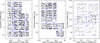 |
Fig. 1 Spatial distribution of galaxies with spectroscopic redshifts 2 < z < 3.5 in three independent VUDS fields: COSMOS (left panel), VVDS-02h (central panel), and ECDFS (right panel). The blue crosses indicate VIMOS pointing centres. |
2.2 Luminosity and stellar mass subsamples selection
Our full sample consists of 3236 objects with reliable spectroscopic redshifts in the range 2 < z < 3.5 observed in three independent fields, COSMOS, VVDS-02h, and ECDFS. These fields cover a total area of 0.92 deg2 , which is the sum of VIMOS slitmask outline after accounting for overlaps (see Fig. 1), corresponding to a volume of ~ 1.75 × 10⁷ Mpc3 . The spatial distribution of galaxies in each field is presented in Fig. 1, while Fig. 2 shows their redshift distribution. The general properties of the whole sample, including the number of galaxies, median redshift, and the effective area, are listed in Table 1.
For the following analysis we selected four volume-limited luminosity subsamples with the selection cuts made in the UV rest-frame absolute magnitudes, computed at a rest wavelength of 1500 (MUV,1500, also denoted as MFUV and further in this work simplified to MUV), and four stellar mass subsamples to study the luminosity and stellar mass dependence of the galaxy clustering, respectively, within the redshift range 2 < z < 3.5. We chose this specific redshift range to be able to study galaxy clustering of as faint galaxies as possible, and at the same time, to maintain volume completeness and large number of galaxies in the various subsamples. In contrast, the choice of the UV wavelength for the luminosity selection is driven by the fact that VUDS is an optically selected survey. The full wavelength coverage of VUDS is 3650–9350 , which corresponds to the UV rest-frame wavelength coverage at redshift ~3.
All of selected subsamples were chosen to contain the number of galaxies sufficient for a reliable measurement of the correlation function based on tests performed on VUDS data prior to this research (see Durkalec et al. 2015b). Selection cuts for different subsamples are shown in Fig. 3. Additionally, general properties of these subsamples including number of galaxies, median redshifts, UV median absolute magnitudes  , and median stellar masses
  of each subsample are listed in Tables 2 and 3.
To account for the mean brightening of galaxies due to their evolution and to ease the comparison between measurements based on samples from various epochs, we normalized the absolute magnitudes and stellar masses, at each redshift, to the corresponding value of the characteristic absolute magnitude  of the Schechter luminosity function in the UV band or to the characteristic stellar mass logM*, respectively. Therefore, for the absolute magnitudes we computed
  , where
  is the original (not corrected) absolute magnitude in the UV filter,
  is the characteristic absolute magnitude, and
  is the characteristic luminosity for galaxies at z = 0. Similar correction was applied for the stellar masses. The values of the characteristic absolute magnitudes were estimated based on the work of Bouwens et al. (2015); Mason et al. (2015); Hagen et al. (2015); Finkelstein et al. (2015); Sawicki & Thompson (2006), while the characteristic stellar masses were taken from Ilbert et al. (2013) and Pérez-González et al. (2008). The details of the methods used to determine the values of characteristic absolute magnitudes and stellar masses at a given redshift are presented in Appendix A.
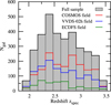 |
Fig. 2 Redshift distribution of the VUDS galaxy sample in the redshift range 2.0 < z < 3.5 used in this study. The filled grey histogram represents the total sample of galaxies, while the red, blue, and green histograms represent the contribution from COSMOS, VVDS-02h, and ECDFS fields, respectively. |
Properties of the galaxy sample in the range 2 < z < 3.5, as used in this study.
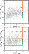 |
Fig. 3 Construction of the volume-limited galaxy subsamples with different luminosity
(upper panel) and stellar mass (lower panel). In both figures the grey dots
represent the distribution of VUDS galaxies as a function of spectroscopic redshift
z.
At each redshift UV
band, absolute magnitudes and stellar masses are normalized to the characteristic absolute magnitudes or to the
characteristic stellar mass, respectively (see Sect. 2.2). The different colour lines delineate the selection cuts
for selected UV
absolute magnitude and stellar mass subsamples as defined in Tables 2 and
3. The dashed black line represents the evolution of the not corrected characteristic
UV
absolute magnitude |

Properties of the galaxy luminosity subsamples, as used in this study.
Properties of the galaxy stellar mass subsamples, as used in this study.
3 Measurement methods
This work isan extension of our previous studies presented in Durkalec et al. (2015b), and all the methods used in this study to quantify thegalaxy clustering are similar to those presented therein. This includes computation techniques, error estimations, analysis of systematics in the correlation function measurements, and correction methods. A detailed description is provided in Sect. 3 of Durkalec et al. (2015b), while below we provide a short summary of the procedures.
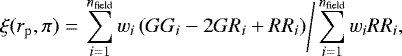
We measured the real-space correlation function ξ(rp, π) of the combined data from three independent VUDS fields through the Landy–Szalay estimator (Landy & Szalay 1993). The differences in size and galaxy numbers between the fields were accounted for by an appropriate weighting scheme. In particular, each pair was multiplied by the number of galaxies per unit volume as follows:
 (1)
(1)
where  and GG, GR, RR are the number of distinct galaxy–galaxy, galaxy–random, and random–random pairs with given separations lying in the intervals of (rp, rp + drp) and (π, π + dπ), respectively. Integrating the measured ξ(rp, π) along the line of sight gives us the two-point projected correlation function wp (rp), which is the two-dimensional counterpart of the real-space correlation function, free from the redshift-space distortions (Davis & Peebles 1983). This correlation function is written as
 (2)
(2)
In practice, a finite upper integral limit πmax has to be used to avoid adding uncertainties to the result. A value that is too small results in missing small-scale signal of correlation function wp(rp), while a value that is too large has the effect of inducing an unjustified increase in the wp (rp) amplitude (see e.g. Guzzo et al. 1997; Pollo et al. 2005). After performing a number of tests for different πmax, we found that wp (rp) is insensitive to the choice of πmax in the range 15 < πmax < 20 h−1 Mpc. Therefore, we chose πmax = 20 h−1 Mpc, which is the maximum value for which the correlation function measurement was not appreciably affected by the mentioned uncertainties.
All correlation function measurements presented in this paper were corrected for the influence of various systematics originating in the VUDS survey properties, by introducing the correction scheme developed in Durkalec et al. (2015b). In particular, we accounted for the galaxies excised from the observations due to the VIMOS layout and other geometrical constraints introduced by the target selection (see Fig. 1). Also, the correcting scheme addresses the possible underestimation of the correlation function related to the small fraction of incorrect redshifts present in the sample and small-scale underestimations observed in tests based on the VUDS mock catalogues.
To estimate the two-point correlation function errors, we applied a combined method (see Durkalec et al. 2015b), which makes use of the so-called blockwise bootstrap resampling method with Nboot = 100 (Barrow et al. 1984) coupled to Nmock = 66 independentVUDS mock catalogues (see Durkalec et al. 2015b; de la Torre et al. 2013, for details about mocks), similar to the method proposed by Pollo et al. (2005). The associated covariance matrix Cik between the values wp on ith and kth scale was computed using
 (3)
(3)
where “⟨⟩” indicates an average over all bootstrap or mock realizations, the  is the value of wp computed at rp = ri in the cone j, where 1 < j < Nmock for the VUDS mocks, and 1 < j < Nboot for the bootstrap data.
Throughout this study we used two approximations of the shape of the real-space correlation function. The first one is a power-law function  , where r0 and γ are the correlation length and slope, respectively. With this parametrization, the integral in Eq. (2) can be computed analytically and wp(rp) can be expressed as
 (4)
(4)
where Γ is the Euler’s Gamma function. Despite its simplicity, a power-law model remains an efficient and simple approximation of galaxy clustering properties.
A second, more detailed description of the real-space correlation function, used here, was performed in the framework of the HOD models. Following a commonly used, analytical prescription, we parametrized the halo occupation model in the way used, for example by Zehavi et al. (2011) and motivated by Zheng et al. (2007). The mean halo occupation function ⟨Ng (Mh)⟩, i.e. the number of galaxies that occupy the dark matter halo of a given mass is the sum of the mean occupation functions for the central and satellite galaxies,
 (5)
(5)
where
![Mathematical equation: \begin{eqnarray*} \langle N_{\textrm{cen}}(M_{\textrm{h}})\rangle & = & \frac{1}{2}\left[1+\textrm{erf}\left(\frac{\log M_{\textrm{h}}-\log M_{\min}}{\sigma_{\log M}}\right) \right], \\ \langle N_{\textrm{sat}}(M_{\textrm{h}})\rangle & = & \langle N_{cen}(M_{\textrm{h}})\rangle \times \left(\frac{M_{\textrm{h}}-M_0}{M_1'}\right)^{\alpha}.\end{eqnarray*}](/articles/aa/full_html/2018/04/aa30734-17/aa30734-17-eq18.png) (6) (7)
(6) (7)
This model includes five free parameters, two of which represent characteristic halo masses that describe the mass scales of haloes hosting central galaxies and their satellites. The characteristic mass Mmin is the minimum mass needed for half of the haloes to host one central galaxy above the assumed luminosity (or mass) threshold, i.e. ⟨Ncen(Mmin)⟩ = 0.5, whereas the second characteristic mass M1 is the mass of haloes that on average have one additional satellite galaxy above the luminosity (or mass) threshold, i.e. ⟨Nsat(M1)⟩ = 1. We note that M1 is different from  from Eq. (7). However, both quantities are related to each other and in most cases
  (see Table 4). The remaining three free parameters are σlog M, which is related to the scatter between the galaxy luminosity (or stellar mass) and halo mass Mh , the cut-off mass scale M0 , and the high-mass power-law slope α of the satellite galaxy mean occupation function.
The HOD parameter space for each galaxy sample has been explored via the population Monte Carlo (PMC) technique (Wraith et al. 2009; Kilbinger et al. 2011), using the full covariance error matrix, as described in Durkalec et al. (2015b). From the best-fitting HOD parameters we derived quantities describing the halo and galaxy properties, such as the average host halo mass ⟨Mh⟩,
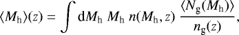 (8)
(8)
the large-scale galaxy bias bg,
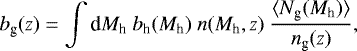 (9)
(9)
and the fraction of satellite galaxies per halo fs
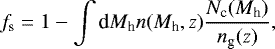 (10)
(10)
where n(Mh, z) is the dark matter mass function, bh(Mh, z) is the large-scale halo bias, and ng(z) represents the number density of galaxies,
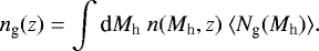 (11)
(11)
4 Results
The two-point projected correlation function wp(rp) was measured in four volume-limited luminosity subsamples and four stellar mass subsamples selected from a totalnumber of 3236 spectroscopically confirmed VUDS galaxies observed in the redshift range 2 < z < 3.5. The composite correlation functions (from three VUDS fields; see Sect. 3) measured for each of these luminosity and stellar mass subsamples are presented in Fig. 4, while the associated best power-law and HOD fits are shown in Fig. 5.
In the case of luminosity limited subsamples, the minimum scale rp that can be reliably measured varies slightly for different galaxy subsamples. For the two faintest subsamples we measure a correlation signal on scales 0.3 < rp < 15 h−1 Mpc, while for the more luminous subsamples it can be measured only on scales 0.5 < rp < 15 h−1 Mpc. We set these particular limits after performing a range of tests on correlation function measured for each of VUDS luminosity subsamples (see Sect. 2.2). The lower rp limit is set at the lowest scale for which, first, we are able to measure a correlation function signal, i.e. wp (rp) has a positive value, and/or, second, we are able to reliably correct (see Durkalec et al. 2015b, for details about the used correction methods) the underestimation of the correlation function that occurs owing to missing close galaxy pairs; this is the result of the low number of galaxies in the sample and/or VIMOS limitations and positions of spectral slits. The maximum scale limit of rp has been chosen as a result of similar tests and under the same conditions. This time, however, the distant galaxy pairs at large rp are missing because of the finite size of VUDS fields.
In practice, we therefore limit our measurement to scales for which the number of galaxy-galaxy pairs in VUDS data is sufficient to measure correlation function with uncertainties that do not exceed the value of wp (rp), and are not affected by volume effects.
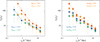 |
Fig. 4 Projected correlation functions for volume-limited samples corresponding to different luminosity (left panel, circles) and stellar mass (right panel, squares) bins, as labelled. |
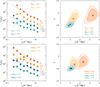 |
Fig. 5 Projected two-point correlation function wp(rp) associated with the best-fitting power-law function (left side) and best-fit power-law parameters r0 and γ along with 68.3% and 95.4% joint confidence levels (right side) in four UV absolute magnitude subsamples (upper panel) and four stellar mass subsamples (lower panel). The symbols and error bars (see Sect. 3 for the error estimation method) denote measurements of the composite correlation function for different luminosity (circles) and stellar mass (squares) subsamples selected from VUDS survey in the redshift range 2 < z < 3.5. For clarity, offsets are applied both to the data points and best-fitting curves of the wp (rp), i.e. the values of wp(rp) and associated best fits for galaxy subsamples with increasing luminosity and stellar masses were staggered by 0.5 dex each. Error contours on the fit parameters are obtained taking into account the full covariance matrix. The 68.3% and 95.4% joint confidence levels are defined in terms of the corresponding likelihood intervals that we obtain from our fitting procedure. |
4.1 Luminosity and stellar mass dependence – power-law fitting of the CF
The best power-law fits of wp(rp), parametrized with two free parameters r0 and γ (see Sect. 3), are presented in the left panel of Fig. 5. The best-fitting parameters for all luminosity and stellar mass subsamples are listed in Table 4 and their 68.3% and 95.4% joint confidence levels are shown in the right panel of Fig. 5.
At redshift z ~ 3 we observe a pronounced dependence of galaxy clustering on both luminosity and stellar mass; the brightest and most massive galaxies are more strongly clustered than their fainter and less massive counterparts (see Fig. 4).
This dependence is reflected in the increase of the correlation length r0 . We find that r0 rises from r0 = 2.87 ± 0.22 h−1 Mpc for the least luminous galaxy subsample (with  ) to r0 = 5.35 ± 0.50 h−1 Mpc for the most luminous galaxies (with
  ). This observed luminosity dependence is systematic, but it becomes more significant for the most luminous galaxies. The correlation functions of the galaxies with increasing luminosities moving from MUV < −19.0 to MUV < −20.0 are very similar at scales rp > 2 h−1 Mpc, which results in a subtle increase in r0 between these subsamples (see Table 4). The rapid growth in the correlation length, by Δ r0 ~ 2 h−1 Mpc, can be observed afterwards for the brightest galaxies (MUV < −20.2).
A similar behaviour occurs for the galaxies selected according to their stellar masses that have a correlation length increasing from r0 = 3.03 ± 0.18 h−1 Mpc for the least massive subsample ( ) to r0 = 4.37 ± 0.48 h−1 Mpc measured for the most massive subsample (
 ). However, in this case the change in the correlation function between subsamples of increasing stellar mass appears to be smoother.
The second of the two free parameters, the slope γ, has also a tendency to grow with increasing luminosity and stellar mass. We find that for the luminosity selected subsamples the value of γ rises from γ = 1.59 ± 0.07 for the faint galaxies to γ = 1.92 ± 0.25 for the brightest galaxies. Similarly, the slope of the power-law fit changes from γ = 1.61 ± 0.06 to γ = 1.82 ± 0.20 for the stellar mass selected subsamples. This increase in the value of γ is likely related to the continuously stronger one-halo term measured for subsamples with increasing luminosities and stellar masses, as discussed below.
4.2 Luminosity and stellar mass dependence – HOD modelling
In the left panel of Fig. 6 we present the measurements of the projected real-space correlation function wp (rp) and the best-fitting HOD models for the four volume-limited UV absolute magnitude (upper panel) and stellar mass (lower panel) subsamples at redshift z ~ 3. As shown, for all selected galaxy samples the best-fitting HOD models reproduce the measurements of the projected correlation function well. However, it is noticeable that in all cases there are some deviations with respect to the model, which predicts correlation function values at large scales (rp > 10 h−1 Mpc) lower than measured. Given the measurement errors, these deviations are more significant for the two least massive and least luminous subsamples. We verified that these deviations are mostly driven by the behaviour of the correlation function measured in the COSMOS field, which is the field with the most galaxies distributed over the largest area in our sample (it comprises of ~ 50% of our galaxy sample; see Table 1), hence with a significant influence on the combined correlation function. The flattening of wp (rp) measured for the COSMOS field at large separations rp > 5 h−1 Mpc can be explained by the presence of an extremely large structure in the COSMOS field, which spans a size comparable to that covered by VUDS-COSMOS (see Appendix B and Cucciati et al., in prep.).
In Table 4 we list the values of the best-fitting HOD parameters (inferred using the full error covariance matrix) with their 1σ errors. Similar to what is seen at lower redshifts (e.g. Zehavi et al. 2011; Abbas et al. 2010; Zheng et al. 2007), we observe a mass growth of the dark matter haloes hosting galaxies with rising luminosity and stellar mass. The minimum halo mass Mmin, for which at least 50% of haloes host one central galaxy, increases from Mmin = 109.73±0.51 h−1 M⊙ to Mmin = 1011.58±0.62 h−1 M⊙ for galaxies with the median UV absolute magnitude  and
and  , respectively. At the same time, for galaxy subsamples selected according to stellar mass, Mmin grows from Mmin = 109.75±0.48 h−1 M⊙ to Mmin = 1011.23±0.56 h−1 M⊙ for galaxies with
  to
to  .
.
We also observe a growth of another characteristic halo mass, M1 , with the luminosity and stellar mass of galaxies. The limiting mass of dark matter halo hosting on average one additional satellite galaxy above the luminosity (or mass) threshold increases from M1 = 1010.33±0.74 h−1 M⊙ for the faintest galaxy subsample to M1 = 1012.29±0.48 h−1 M⊙ for the most luminous galaxies. Similarly, for the stellar mass selected subsamples M1 rises from M1 = 1010.21±0.69 h−1 M⊙ to M1 = 1011.57±0.65 h−1 M⊙ from the less to the most massive galaxy subsamples, respectively.
These changes, both, of the minimum Mmin and satelliteM1 masses of dark matter haloes hosting galaxies with different properties are in agreement with the predictions of the hierarchical scenario of structure formation as discussed in Sect. 5.3.
Additionally, we observe an increase with luminosity of the high-mass slope α of the satellite occupation in the UV absolute magnitude selected galaxy subsamples. For the two brightest subsamples (MUV < −20.0 and MUV < −20.2) α is noticeably higher α =1.95 ± 0.23, than observed for the fainter galaxy populations, where α takes values around unity. This observed difference is likely related to the more pronounced one-halo term for the most luminous galaxy sample. It indicates that satellite galaxies are more likely to occupy most massive dark matter haloes. The situation is less clear for the stellar mass selected subsamples, where, given the measurement uncertainties, we do not observe any significant change in the slope α for the four different stellar mass subsamples.
All these differences in the HOD parameter values measured for galaxy populations with different luminosities and stellar masses are reflected in the evolution of the halo occupation function presented in the right panels of Fig. 6. The halo occupation function shifts towards higher halo masses when going towards brighter and more massive galaxy subsamples showing that more luminous and more massive galaxies, respectively, occupy more massive haloes. For the luminosity selected subsamples this shift of the halo occupation function is rather continuous, while for the stellar mass selected galaxies there is a rapid 1 dex increase in halo masses moving from the two least massive to the two most massive galaxy populations.
Such a rapid shift in the halo mass related to a relatively small change in the stellar mass has not been reported in the literature. At z ~ 2 McCracken et al. (2015), based on the angular correlation function measurements, finds a continuous growth of both minimum (from Mmin ~ 1012.4 M⊙ to Mmin ~ 1012.6 M⊙) and satellite halo masses (from M1 ~ 1013.45 M⊙ to M1 = 1014.0 M⊙) for galaxies with stellar masses ranging from  to
to  . Similarly, at z ~ 1.5 Hatfield et al. (2016) measured a steady increase in the minimum halo mass by Δ logMmin = 0.5 M⊙ for subsamples of galaxies with stellar masses from
  to
to  . These studies, however, do not cover stellar masses smaller than
  , which is the threshold limit of the most massive galaxy subsample used in this work.
The presence of the halo mass discontinuity with respect to the increasing stellar mass of galaxies and lack of such discontinuity observed for luminosity selected subsamples suggests that the relationship between the luminosity of a galaxy and the corresponding halo mass significantly differs from the relationship between its stellar mass and the mass of the dark matter halo. This in turn implies that the processes determining the galaxy luminosity, even if related to the evolution of the hosting halo, could be more complex than the relation between the halo and galaxy stellar mass.
The observed discontinuity in halo mass, with respect to small difference in stellar mass, directly influences the observed stellar-to-halo mass relation. In particular we observe that, at z ~ 3, low-mass end of this relation deviates from the theoretical predictions by, for example Behroozi et al. (2013) and Moster et al. (2013). We discuss the possible implications of this result in more detail in Sect. 5.5.
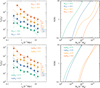 |
Fig. 6 Projected two-point correlation function wp(rp) associated with the best-fitting HOD models (left side) and evolution of the halo occupation function of the best-fit HOD model (right side) in four UV absolute magnitude subsamples (upper panel) and four stellar mass subsamples (lower panel). The symbols and error bars (see Sect. 3 for the error estimation method) denote measurements of the composite correlation function for different luminosity (circles) and stellar mass (squares) subsamples selected from the VUDS survey in the redshift range 2 < z < 3.5. For clarity, offsets are applied to both the data points and best-fitting curves of the wp (rp), i.e. the values of wp(rp) and associated best fits for the galaxy subsamples with increasing luminosity and stellar masses were staggered by 0.5 dex each. |
5 Discussion
5.1 Dependency of galaxy clustering on their luminosity and stellar-mass
Our most important conclusion is that at redshift z ~ 3 galaxy clustering depends on luminosity and stellar mass. As presented in Fig. 4 and described in Sect. 4.1, we observe a constant increase of r0 from faint and low massive samples to the most luminous and the most massive samples. This implies that at high redshift the most luminous and most massive galaxies are more strongly clustered than their fainter and less massive counterparts and that a higher clustering is observed on both small and large spatial scales.
This luminosity and stellar mass dependence of galaxy clustering can be explained in the framework of the hierarchical mass growth paradigm. In this scenario, the mass overdensities of the density field collapsed overcoming the cosmological expansion. The initiallystronger overdensities grew faster, hence their stronger clustering pattern imprinted in the dark matter density field. With time, the resulting dark matter haloes merged together, forming larger haloes, which served as the environment in which galaxies formed and evolved (Press & Schechter 1974; White 1976). The strongest and most clustered overdensities produced the largest haloes, containing the corresponding amount of baryons, which – in turn – agglomerated to produce the largest and most massive (consequently also the most luminous) galaxies. This behaviour is reflected in the N-body simulations complemented by semi-analytical models, which show that the galaxy luminosity and stellar mass are tightly correlated with the mass of their haloes. In consequence, the clustering of a particular galaxy sample is expected to be largely determined by the clustering of haloes that host these galaxies (Conroy et al. 2006; Wang et al. 2007).
This simple picture, however, complicates when we need to take the evolution of galaxies, driven by baryonic physics, into account. This makes it more difficult to predict how exactly luminosity and stellar mass dependence of galaxy clustering changes with time. In particular, star formation occurs only after baryonic matter reaches a certain critical density and proceeds in a different way depending, for example on the initial galaxy mass, halo mass, and interactions with other galaxies (see e.g. White & Rees 1978; De Lucia et al. 2007; López-Sanjuan et al. 2011; Tasca et al. 2014). Therefore, the evolution of luminosity and stellar mass clustering dependence is not only related to the growth of dark matter halo masses, but also to the physics of baryons that make up the galaxies. We expect that for the most massive galaxies occupying the most massive dark matter haloes, the build up of stellar mass is eventually limited by various feedback effects (e.g. Blanton et al. 1999), while the less massive galaxies occupying less massive dark matter haloes continue to form stars (downsizing; see e.g. De Lucia et al. 2006). In consequence, we expect to observe a strong luminosity and stellar mass dependence of galaxy clustering at z ~ 3 and its weakening with time.
However, the question of whether there is a differential evolution between low and high luminosity galaxies or low and high stellar mass galaxies from z ~ 3 to z ~ 0 remains open. It is difficult to compare the strength of galaxy clustering at different redshifts. The clustering amplitudes observed at different epochs cannot be easily related because of the differences in the selection methods used to sample galaxies in different surveys, which in turn results in sampling different galaxy populations at different redshifts. Still, we find that our results, which indicate that a higher clustering amplitude observed for more luminous galaxies on both small and large spatial scales rp , are consistentwith the results based on the data from low (e.g. the SDSS survey, Zehavi et al. 2011; Guo et al. 2015, the 2dF survey, Norberg et al. 2002) and intermediate (e.g. the DEEP2 survey, Coil et al. 2006, the VVDS survey, Pollo et al. 2006; Abbas et al. 2010, the zCOSMOS, Meneux et al. 2009, the VIPERS survey, Marulli et al. 2013) redshift ranges. For example, based on the large SDSS z ~ 0 galaxy sample Zehavi et al. (2011) found that the correlation length increases by Δ r0 ~ 6.5 h−1 Mpc between galaxies with Mr < −18.0 and Mr < −22.0. Moreover, similar to our work, the luminosity dependence is more pronounced for bright samples and less significant for the fainter samples (see Sect. 4.1). At intermediate redshift ranges, for example Marulli et al. (2013) analysing data from the VIPERS survey, found that at z ~ 1 the correlation length increases from r0 = 4.29 ± 0.19 h−1 Mpc to r0 = 5.87 ± 0.43 h−1 Mpc for galaxies with MB < −20.5 and MB < −21.5, respectively. Consistent with these findings at lower redshifts, also at z ~ 3, we find a Δr0 ~ 2.5 increase between the faintest (MUV < −19.0) and the brightest (MUV < −20.2) galaxies and a Δr0 ~ 1.5 increase between stellar mass selected subsamples. As mentioned at the beginning of this paragraph, because all these measurements possibly consider different galaxy populations, we are not able to draw a detailed conclusion about whether or not luminosity and stellar mass clustering dependence is stronger (or weaker) at high redshift in comparison to the local Universe. What can be safely said, however, is that dependence of clustering with luminosity and stellar mass is present and strong at z ~ 3, as it is observed at z ~ 0 (Δ r0 of the same order of magnitude at both redshifts), and therefore much of the processes that produced luminosity and stellar mass clustering dependence must have been at work at significantly higher redshift than z ~ 3.
5.2 Relative and large-scale galaxy bias of different luminosity and stellar mass subsamples
Using the best-fitting power-law parameters r0 and γ, we interpretour results in terms of the relation between the distribution of galaxies and the underlying dark matter density field for galaxy populations with different luminosities. We compare the values of the relative galaxy bias b∕b* measured from the VUDS survey to the bias of galaxy populations with different luminosities measured at lower redshift ranges, taken from the literature.
The relative bias parameter, b∕b*, is based on the amplitude of the correlation function relative to that of L* galaxies and can be defined as the relative bias of the generic ith sample with a given median luminosity Lmed, with respect to that corresponding to L*, as
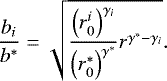 (12)
(12)
In our study we use a fixed scale r = 1 h−1 Mpc (see also Meneux et al. 2006, for a slightly different definition). To apply this formula, first we need to estimate the values of  and γ* for
  galaxies. We obtain them through a linear fit to the relation between correlation length and absolute magnitude of the sample normalized to the characteristic absolute magnitude at median redshift
  and
and  measured in this work.
Figure 7 shows the relative bias measured for the VUDS galaxies with the luminosities sampled at z ~ 3 compared to various results at lower redshifts, along with the analytic fit of the 2dFGRS data b∕b* = 0.85 + 0.16L∕L* from Norberg et al. (2002) and b∕b* = 0.85 + 0.15L∕L*− 0.04(M − M*) based on the SDSS sample (Tegmark et al. 2004).
In each luminosity subsample the relative bias at z ~ 3 of galaxies with Lmed∕L* < 1 is significantly lower than that observed at lower redshifts for galaxies with similar Lmed∕L* ratios. However, none of our subsamples have Lmed > L*; thus we cannot exclude the possibility that for galaxies with Lmed > L* the relative bias would be higher, which is very likely, taking into account the trend visible in Fig. 7. Additionally, we observe that the value of b∕b* rises more steeply with Lmed∕L* for high redshift galaxies than observed locally. At z ~ 3 the relative bias increases from low values b∕b* = 0.42 ± 0.03 at low luminosities to b∕b* = 0.85 ± 0.11 for the high luminosity subsample. Pollo et al. (2006) found a similar steep growth of the relative bias for galaxies observed at z ~ 1. At z ~ 0, instead, b∕b* increases only by ~0.1 in the same Lmed∕L* interval, following the model from Norberg et al. (2002). This appears to be an indication that going back in time the bias contrast of the most luminous galaxies with respect to the rest of the population becomes stronger and is consistent with the fact that fainter galaxies are found to be significantly less biased tracers of the mass than brighter galaxies even at high redshifts. However, we need to take into account the possibility that the observed strengthening of b∕b* relation with luminosity at higher redshifts can also be partially attributed to a more pronounced one-halo term at higher z making the power-law fit of the clustering measurement less reliable.
In orderto break this ambiguity, we use the best-fitting parameters of the HOD model to estimate the large-scale galaxy bias bg,HOD, using Eq. (9). The results obtained for the luminosity and stellar mass subsamples at z ~ 3 are given in Table 4 and presented in Fig. 8, where for comparison we also plot the results obtained at lower redshifts. For both, the UV absolute magnitude and stellar mass selected subsamples, the values of bg,HOD measuredat z ~ 3 are significantly higher than locally, indicating that in the early stages of evolution galaxies are highly biased tracers of the underlying dark matter density field. As shown in the right panel of Fig. 8, the galaxy bias decreases systematically with cosmic time for all stellar masses extending to z > 3, that is the trend found at lower redshifts (e.g. McCracken et al. 2015). The observed decrease in the galaxy bias with cosmic time can be explained in terms of the hierarchical scenario of structure formation. At early epochs the first galaxies are expected to form in the most dense regions, resulting in a high bias with respect to the underlying average mass density field. As the mass density field evolves with time, these regions grow in size and mass, the gas trapped inside becomes too hot to collapse, effectively preventing the formation of new stars (e.g. Blanton et al. 1999) and resulting in galaxy formation systematically moving to less dense, hence less biased, regions.
In addition to the redshift dependence of galaxy bias and in agreement with previous studies at lower redshifts (e.g. Norberg et al. 2002; Tegmark et al. 2004; Meneux et al. 2008; Zehavi et al. 2011; Mostek et al. 2013), we observe a clear luminosity and stellar mass bias dependence, in which the brightest and most massive galaxies are the most biased.
In the left panel of Fig. 8 we show the large-scale galaxy bias bg,HOD as a function of luminosity and compare this bias with the similar results from Zehavi et al. (2011). As presented, at z ~ 0 the luminosity dependence of bias is nearly flat for galaxies with luminosities L ≤ L* and then rises at brighter luminosities. According to Zehavi et al. (2011) this relation is best fitted by the functional form  . We adopt a similar formula to model the galaxy bias–luminosity relation, and at z ~ 3 we find that for the luminosity threshold samples bg,HOD(>L) is best fitted by
 (13)
(13)
which is represented by a solid line in the left panel of Fig. 8. Here L is the UV luminosity and L* corresponds to the characteristic absolute magnitude  obtained as described in Appendix A. Our estimate of the dependence of the large-scale bias on galaxy luminosity is nearly flat for galaxies with luminosities L ≤ 0.5L* and rises very sharply for brighter galaxies. Therefore, in agreement with the analysis of the relative bias discussed above, this suggests that the bias contrast between bright and faint galaxies becomes stronger when going back in time.
In the right panel of Fig. 8 we also present the large-scale galaxy bias measurements for the stellar mass selected subsamples. We compare our results with the similar measurements at z ~ 0.5 from Skibba et al. (2015; open circles), at z ~ 1 from Mostek et al. (2013; filled triangles), and from McCracken et al. (2015) over the redshift 0.5 < z < 3.5 (black lines), based on the large PRIMUS, DEEP2, and UltraVISTA galaxy samples, respectively. In addition to the bg values at z ~ 3 being higher than observed at lower redshifts (discussed earlier), we find that the galaxy bias rises towards more massive galaxies from bg,HOD = 1.99 ± 0.58 measured for galaxies with Mmed = 109.48 h−1 M⊙ to bg,HOD = 2.84 ± 0.99 for the most massive galaxy subsample with Mmed = 1010.24 h−1 M⊙. These galaxy bias values are also in excellent agreement with measurements based on N-body simulations performed by Chiang et al. (2013), who at z = 3 find bg = 2.24 and bg = 2.71 for galaxies with stellar masses M > 109 M⊙ and M > 1010 M⊙, respectively. As for the luminosity selected galaxies, we made an attempt to model this bias-stellar mass relation at z ~ 3. We find that the best-fitting function, represented in Fig. 8 by a solid line, is given by
 (14)
(14)
where M is the galaxy stellar mass and M* is the characteristic stellar mass at z ~ 3.
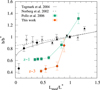 |
Fig. 7 Relative bias b∕b* (see Eq. (12)) for the selected VUDS luminosity subsamples at z ~ 3 (orange circles) as a function of luminosity with L* as a reference point. The results from this work are compared to similar studies at lower redshift ranges: at z ~ 0.1 from Zehavi et al. (2011) (filled black circles) and Norberg et al. (2002) (black crosses), and at z ~ 0.9 from Pollo et al. (2006) (green circles). The lines indicate the analytic fit of the 2dFGRS data from Norberg et al. (2002) (black solid line) and SDSS data from Tegmark et al. (2004) (black dashed line), as described in the text. |
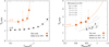 |
Fig. 8 Large-scale galaxy bias bg,HOD as a functionof luminosity, with L* as a reference point (left panel) and as a function of stellar mass with M* as a reference point (right panel). In both plots, the coloured points indicate measurements at z ~ 3 from this work; the solid lines indicate the best-fit functions of the bias-luminosity dependence bg,HOD(>L) (Eq. (13)) and bias-stellar mass dependence bg,HOD(>M) (Eq. (14)) as described in Sect. 5.2. In the left panel, the black circles show the results from Zehavi et al. (2011) at z ~ 0 and the dashed line represents the empirical fit of the bias-luminosity dependence in the functional form given therein. In the right panel, we show for comparison the bg measurements at z ~ 0.5 from Skibba et al. (2015) represented by open circles, those at z ~ 1 by Mostek et al. (2013) are indicated by black triangles and from different samples in the redshift range 0.5 < z < 2.5 measured by McCracken et al. (2015) shown as black lines as labelled. |
5.3 Halo masses of different galaxy populations
In Fig. 9 we show the values of two characteristic halo masses, Mmin and M1 , in terms of the sample threshold luminosity (left panel) and stellar mass (right panel) relative to the characteristic luminosity and stellar mass, Lthresh∕L* and Mthresh∕M*, respectively, at different redshifts. The minimum halo mass needed for half of the haloes to host one central galaxy above the luminosity or stellar mass threshold Mmin (filled symbols) and the mass of haloes with on average one additional satellite galaxy above the luminosity or stellar mass threshold M1 (open symbols), measured at z ~ 3 are compared with similar results at z ~ 0 from Zehaviet al. (2011), represented by dashed and dotted lines, respectively. As shown, the values of both Mmin and M1 at z~ 3 for all galaxy luminosities are lower than measured in the local Universe. This observation suggests that to hostat least one central galaxy, above the luminosity or stellar mass threshold, the dark matter haloes at low redshift need to accumulate a larger amount of mass than is seen at higher redshifts.
In Sect. 4.2 we noted that minimum halo masses grow with increasing luminosity and stellar mass of the galaxy sample. Similar growth is reported at lower redshifts (e.g. Zheng et al. 2007; Abbas et al. 2010; Zehavi et al. 2011; Coupon et al. 2012; de la Torre et al. 2013); however, as presented in Fig. 9, at z ~ 3 the contrast between halo masses of faint and bright galaxies is much larger than observed in the local Universe for galaxies with similar Lthresh∕L*. This impliesthat at high redshift the bright and most massive galaxies are much more likely to occupy the most massive dark matter haloes. Combining this with the earlier observation that a lower mass dark matter halo is needed to host a galaxy of higher luminosity/stellar mass at higher redshift suggests that the processes responsible for the subsequent increase of the mass of the halo and stellar mass of the galaxies operate on different timescales and are both stellar mass and epoch dependent.
With the increasing Mmin we observe a proportional growth of M1. At all luminosities the values of Mmin and M1 present an approximately constant ratio M1∕Mmin ≈ 4 . This indicates that at z ~ 3 the halo hosting one central and one satellite galaxy (above a luminosity threshold) needs to be only four times more massive than the halo that hosts only one central galaxy. For the stellar mass selected subsamples, this factor is even smaller M1 ∕Mmin ≈ 2.5. For comparison, in the local Universe theratio between M1 and Mmin is higher. At z ~ 0 Zehavi et al. (2011) found the scale factor M1 ≈ 17Mmin for the SDSS galaxies selected by their r-band absolute magnitude, while at intermediate redshift z ~ 1 Zheng et al. (2007) and Skibba et al. (2015) observed a slightly lower factor of ≈ 15 and McCracken et al. (2015) reported values of ≈10 for galaxies at 1.5 < z < 2.0. These results, combined with our observations at z ~ 3, can be interpret as evidence that, firstly, at higher redshifts dark matter haloes consist of many recently accreted satellites, and secondly, the M1∕Mmin ratio evolves with redshift with lower values observed at higher redshifts; this finding is in agreement with other studies (e.g. de la Torre et al. 2013; Skibba et al. 2015; McCracken et al. 2015) and can be explained by the relation between halo versus galaxy merging (Conroy et al. 2006; Wetzel et al. 2009). The dark matter halo mergers create an infall of satellite galaxies onto a halo, while the galaxy major mergers destroy these halos. If the halo mergers occur more often than the galaxy mergers, we can expect a large satellite population, resulting in a small M1 ∕Mmin ratio.
According to the high-resolution N-body simulations performed by Wetzel et al. (2009), at z > 2.5 the merger rate of subhaloes (effectively galaxies) is significantly lower than that of haloes. For example, at z ~ 3 haloes of mass Mh ≈ 1012 h−1 M⊙ are expected to experience ~0.9 mergers/Gyr, compared to only ~0.4 mergers/Gyr expected for subhaloes; based on a preliminary VUDS sample Tasca et al. (2014) found an even lower value of major galaxy mergers, i.e. 0.17 mergers/Gyr. This implies that at z > 2.5 the satellite galaxies are created faster than they are destroyed. Moreover, the halo versus galaxy merger ratio decreases with time and at z < 1.6 the two merger rates are approximately the same. Therefore, there is an expected rapid rise in the satellite halo occupation at redshifts higher than z ~ 2 and its slow levelled evolution afterwards. Simulation predictions from Wetzel et al. (2009) are indirectly confirmed by our measurements. The high number of satellites per halo at high redshift is reflected in the small ratio of M1 ∕Mmin, while a smaller halo occupation at lower redshift corresponds to its increase with time.
From the observational side the galaxy major merger rate has been shown to rapidly rise from z ~ 0 to z ~ 1.5 (e.g. de Ravel et al. 2009; López-Sanjuan et al. 2011, 2013) and to decrease for higher redshifts z > 2 (Tasca et al. 2014). This indicates that the peak of galaxy merging activity occurred around z ~ 1.5–2 (see also Conselice et al. 2008), hence later than the lower redshift limit of our galaxy sample. These observational results combined with large-scale N-body simulations predictions, mentioned earlier, might explain the observed low value of M1 ∕Mmin at z ~ 3 and its increase with cosmic time.
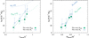 |
Fig. 9 Characteristic halo masses from the best-fitting HOD models of the correlation function selected in luminosity vs. Lthresh∕L* (left panel) and selected in stellar mass vs. Mthresh∕M* (right panel). Minimum halo masses Mmin for which 50% of haloes host one central galaxy above the threshold limit (filled symbols) and masses of haloes which on average host one additional satellite galaxy M1 (open symbols) observed at z ~ 3 are compared with similar results found by Zehavi et al. (2011) at z ~ 0, for the luminosity selected galaxies, and by Skibba et al. (2015) at z ~ 0.5, for the stellar mass selected galaxies (dotted and dashed lines). |
5.4 Satellite fraction
We compute the fraction of satellite galaxies per halo fs for all luminosity and stellar mass subsamples using the HOD best-fitting parameters (Eq. (10)). The results, as a function of threshold luminosity with L* is a reference point (left panel) and threshold stellar mass with M* a reference point (right panel), are shown in Fig. 10. We compare our measurements at z ~ 3, represented by filled symbols with similar results obtained at z ~ 0 by Zehavi et al. (2011) (left panel, dashed line) and at z ~ 0.5 by Skibba et al. (2015) (right panel, open triangles).
These results have implications for satellite abundances as a function of luminosity and stellar mass, as well as a function of redshift. At z ~ 3 we observe a luminosity dependence of satellite abundance. The satellite fraction drops from ~ 60% for the faintest galaxy population to ~20% for the brightest galaxies. A lower value of fs for the brightest galaxies does not necessarily mean that there are no other satellite galaxies occupying a dark matter halo, but rather that there are no bright satellite galaxies. Therefore, our results would suggest that, at high redshift it is more probable that a dark matter haloes host faint satellite galaxies, rather than very bright galaxies. A similar, however less steep, trend is present in the local Universe (Zehavi et al. 2011). The situation is less clear for galaxies selected according to their stellar mass. Taking into account the uncertainties of our measurement, we are not able to determine if fs changes with the stellar mass of galaxies, as observed at lower redshift ranges (Skibba et al. 2015). At face value our data suggest the possible presence of a small drop, by Δfs ~ 0.1, from the least massive to the most massive galaxies, but it is not a significant change (at the level of 0.5σ).
From the perspective of the redshift evolution, we observe that the satellite fraction of the two faintest galaxy subsamples and of all the stellar mass selected galaxy subsamples is higher at z ~ 3 than it is observed at lower redshift. This means that at high redshift it is more likely that a halo hosts a satellite galaxy above a given threshold limit, than locally. This high satellite abundance observed for star-forming galaxies with L ~ L* at high redshift can be explained using the same reasoning as presented in Sect. 5.3. This high abundance suggests that the infall of the satellite galaxies, as a result of halo mergers, onto a dark matter halo is faster than their destruction via galaxy major mergers (Wetzel et al. 2009). Therefore, the subhaloes that form after halo mergers are likely to remain intact and this leads to a large number of satellite galaxies at high redshift, resulting in the measured high satellite fraction. It is necessary to mention, however, that this conclusion applies to star-forming galaxies, with L ~ L*, as the used data sample does not include a population of faint galaxies at z ~ 3.
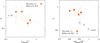 |
Fig. 10 Satellite fraction fs as a functionof threshold luminosity, with L* as a reference point (left panel) and as a function of threshold stellar mass, with M* as a reference point (right panel). Results obtained in this work at z ~ 3 (filled symbols) are compared with similar measurements from lower redshift ranges. In the left panel the dashed line indicates the satellite fraction as measured at z ~ 0 by Zehavi et al. (2011), while in the right panel results found by Skibba et al. (2015) at z ~ 0.5 are shown with open triangles. |
5.5 Stellar to halo mass relation for low-mass galaxies
In this section we focus on the relationship between halo mass and stellar mass of each galaxy sample, in the literature simply referred to as the stellar-to-halo mass relation (SHMR; see e.g. Behroozi et al. 2010, 2013; Moster et al. 2013; Leauthaud et al. 2012; Yang et al. 2012; Durkalec et al. 2015a).
In Fig. 11 we present the SHMR at z ~ 3 for all stellar mass subsamples used in this paper (filled squares). Owing to the construction of the subsamples (threshold limited) and the halo occupation model used, we plot the parameter Mmin to represent the halo mass associated with the threshold stellar masses  of the galaxy subsamples. The errors associated with the stellar mass threshold limit are computed as the average of the errors on M⋆ for each stellar mass subsample separately.
We compare our results with the z = 3 theoretical model predictions by Behroozi et al. (2013) and Moster et al. (2013), which both use the abundance matching method to infer stellar-to-halo mass relation, and with models by Yang et al. (2012), which are based on galaxy clustering and HOD modelling. We find that, for the massive galaxies, with stellar masses M⋆ > 109.75 M⊙ our results are in agreement with these models. However, for galaxies with low stellar masses (M⋆ < 109.25 M⊙), there is a striking difference between our z ~ 3 measurements of SHMR and the theoretical model predictions. For these galaxies all models predict significantly more massive (by 1 dex) dark matter haloes than inferred from our measurements. For instance, we estimate haloes of Mh= 109.75 M⊙ hosting galaxies with minimum stellar masses of  , while modelpredictions by Behroozi et al. (2013) place the same galaxies in much more massive haloes of Mh~ 1011 M⊙. In other words, we observe that the low-mass galaxies at z ~ 3 have formedstars more efficiently than it is expected from these models, which all assume a much steeper decrease of the effective star formation with decreasing halo mass.
Such discrepancies between model predictions and observational constraints at high redshift have not been reported before in the literature. For example, in our previous studies (Durkalec et al. 2015a) based on the preliminary VUDS observations and for subsamples covering a wider redshift range (2.0< z < 5.0), and higher stellar masses, we found the SHMR in broad agreement with theoretical model predictions. At z ~ 2 for numerous stellar mass subsamples, McCracken et al. (2015) compared the HOD based SHMR measurements with the abundance matching based models and found them to be in broad agreement. Similarly, at z = 3, Ishikawa et al. (2017) have reported an excellent agreement of their SHMR measurements with the model predictions by Behroozi et al. (2013) for a large Lyman break galaxy (LBGs) sample. It is important to note, however, that galaxies used in these studies do not reach the stellar mass range below M⋆ = 109.1 M⊙2, while the stellar mass limit of our least massive subsample is significantly smaller (108.75 M⊙). The same limitation applies to the theoretical models of SHMR at high redshift, which are not constrained by observations at the low stellar mass end (e.g. the SHMR model by Behroozi et al. 2013, at z = 3 is constrained only down to M⋆ = 109.4 M⊙).
The SHMR is most commonly parametrized either with a double power-law function (Behroozi et al. 2010; Yang et al. 2012; Moster et al. 2013), or with a the five parameter function proposed by Behroozi et al. (2013), which retains a power-law form for halo masses Mh ≪ 1011.97 at z = 3. Our results suggest that, at high redshifts, this power-law shape is broken at the low-mass end below Mh = 1011 M⊙ (see Fig. 11). In particular, according to our measurements, the stellar to halo mass ratio is higher than predicted for this halo mass range. This is in agreement with the conclusion by Behroozi et al. (2013) who note that the low-mass end of the SHMR cannot be predicted by extrapolating results from massive galaxies and fit with the power-law function alone.
A similar higher-than-expected stellar mass to halo mass ratio is observed for dwarf galaxies (e.g. Boylan-Kolchin et al. 2012; Ferrero et al. 2012; Miller et al. 2014; Brook et al. 2014; Read et al. 2017). The low-mass galaxy subsamples used in this paper are not as low mass as the dwarf galaxies observed in the local group; the minimum stellar mass of VUDS galaxies used in our sample is M⋆ = 108.75 M⊙, while the masses of local dwarf galaxies are 106–109 M⊙. However, the low-mass observation-model discrepancy of SHMR we observe is consistent with these low-mass low redshift samples and it is possible that similar processes are behind it at high z for the higher mass galaxies.
A possible explanation of the discrepancy between the observed SHMR of low-mass galaxies and models may lie in the flaws of the abundance matching technique (used in the presented theoretical models to infer SHMR) coupled with our still poor understanding of the feedback effects that influence not only the galaxy stellar mass assembly, but also the mass distribution of the hosting dark matter haloes (e.g. Pontzen & Governato 2012; Di Cintio et al. 2014; Ogiya & Mori 2014; Katz et al. 2017). The abundance matching technique uses simulated dark matter distributions. It is well known, however, that N-body simulations predict a dark matter halo mass function much steeper than the galaxy stellar mass function derived from observations(Press & Schechter 1974; Jenkins et al. 2001; Sheth et al. 2001; Springel et al. 2005). Moreover, this difference increases while moving towards low, both stellar and halo, mass regimes (our point of interest here). This difference is usually reconciled by assuming that galaxy formation is directly connected to the fact that halo mass and galaxies do not form efficiently in low-mass haloes. This leads to an overestimation of halo masses for low-mass galaxies, when the galaxies are matched with haloes under the assumption that dark matter-only simulations represent structure formation and that every halo hosts a galaxy, which is the case in the abundance matching method. This overestimation of the halo masses derived by models, with respect to the observations, is the one visible in Fig. 11 for the galaxies with M⋆ < 109.5.
The relation between dark matter halo mass and galaxy stellar mass is therefore not direct. It can be additionally influenced by, for example the strong feedback effects, which affect the star formation in low-mass galaxies more strongly than in more massive galaxies. In particular the strong positive feedback (either SN or AGN originated) would result in higher than expected star formation efficiency of low-mass galaxies visible as the model-observation discrepancy for these galaxies in Fig. 11.
At low redshifts the feedback effects have been proposed to have a major impact on the evolution of dwarf galaxies (see e.g. Ferrara & Tolstoy 2000; Fujita et al. 2004; Mashchenko et al. 2008; Sawala et al. 2011; Kawata et al. 2014; Oñorbe et al. 2015; Chen et al. 2016; Papastergis & Shankar 2016). Our SHMR measurements, i.e. the higher than expected star formation efficiency, suggest that at z ~ 3 a positive feedback effects have a significant influence on stellar mass assembly in not only dwarf galaxies (M⋆ < 109), as it is observed locally, but also in more massive galaxies, which at z = 0 are not observed to be strongly affected. This conclusion can be supported by the fact that a strong feedback effects, bothpositive and negative, has been observed in abundance in nearly all star-forming galaxies at high z (e.g. Pettini et al. 2001; Shapley et al. 2003; Weiner et al. 2009; Steidel et al. 2010; Jones et al. 2012; Newman et al. 2012; Erb 2015; Talia et al. 2017; Le Fèvre et al. 2017).
However, we note that other processes might be at work, hence this interpretation may not be the only one and that only further observations of low-mass high redshift galaxies might help to resolve the problem. For example, positive feedback might not be sufficient to alleviate model to observations at low-mass end, and we need to account also for the possible existence of so-called dark haloes, i.e. haloes that are completely devoid of stars (see e.g. Sawala et al. 2013, 2015). A high number of such haloes would strongly affect the accuracy of models based on the abundance matching techniques. Also, regardless of the fact that introducing a strong positive feedback in low-mass galaxies at high redshifts is physically motivated, it might not produce the correct star formation histories, resulting in a more numerous population of passive galaxies than is observed locally, as suggested by, for example Fontanot et al. (2009); Weinmann et al. (2012), and Moster et al. (2013). We, therefore, conclude that a mixture of both effects, i.e. strong positive feedback effects and a high number of empty dark matter haloes is a possible explanation of the observed trends.
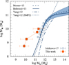 |
Fig. 11 Stellar mass–halo mass relation (SHMR) of central galaxies obtained for different stellar mass selected subsamples
at z ~ 3
(orange symbols). The halo masses are represented by the best-fit parameter
Mmin ,
while the associated stellar masses of the galaxies are represented by the threshold limits
|

6 Summary and conclusions
In this paper we study the luminosity and stellar mass dependence of galaxy clustering at redshift z ~ 3 using a large spectroscopic sample of 3236 star-forming galaxies from the VUDS survey. We measure the real-space correlation function wp (rp) in four volume-limited luminosity subsamples, with the cuts made in UV absolute magnitude, and four stellar mass subsamples. Our measurements are quantified in the framework of two approximations. The first is the power-law model  with two free parameters. The second is based on the HOD model with five free parameters.
The main results and conclusions of our study can be summarized as follows:
-
We observe an increase of the correlation length r0 with the luminosity and stellar mass of the galaxy populations, indicating a luminosity and stellar mass dependence of galaxy clustering at z ~ 3. For UV luminosity selected subsamples r0 rises from r0 = 2.87 ± 0.22 h−1 Mpc to r0 = 5.35 ± 0.50 h−1 Mpc over a threshold UV absolute magnitude ranging from MUV = −19.0 to MUV = −20.2. A similar trend is found for stellar mass selected galaxy samples, where the correlation length grows from r0 = 3.03 ± 0.18 h−1 Mpc to r0 = 4.37 ± 0.48 h−1 Mpc over a relatively small stellar mass range ΔlogM⋆ = 1.25 h−1 M⊙. Based onthese observations we conclude that at z ~ 3 the luminous and most massive galaxies exist preferentially in denser regions of the Universe than their less luminous and less massive counterparts. This trend is consistent with similar trends reported at lower redshifts and is still strong at z ~ 3. It indicates that mechanisms that led to luminosity and stellar mass clustering dependence must have been at work at a significantly higher redshift than z ~ 3.
-
Based on the power-law approximation of the correlation function, we interpret our results in terms of the relation between the distribution of galaxies and the underlying dark matter density field, called bias (b), relative to the b* of the L* galaxies. We note that at z ~ 3 the measured values of b∕b*, in each luminosity subsample, are significantly lower than observed for the local and intermediate redshift ranges for galaxies of similar properties. Additionally, we observe that the relative galaxy bias grows with the increasing luminosity of the sample from low values b∕b* = 0.41 ± 0.03 at low luminosities to b∕b* = 0.86 ± 0.1 for the high luminosity subsample. This growth of b∕b* at z ~ 3 with luminosity is much steeper than measured for local galaxies, indicating that going back in time the bias contrast of the most luminous galaxies to the rest of the population was stronger. This is consistent with the fact that fainter galaxies are found to be significantly less biased tracers of the mass than the brighter galaxies, now confirmed at high redshifts.
-
Taking advantage of the HOD best-fitting parameters we measure the large-scale galaxy bias bg,HOD. We interpret our results in terms of both redshift evolution and as a function of luminosity and stellar mass. As expected in the framework of the hierarchical scenario of structure formation and evolution, we observe that the bg,HOD measured at z ~ 3 is significantly higher than locally, indicating that in the early stages of the evolution of the Universe galaxies were more biased tracers of the underlying dark matter density field than is currently observed. In addition to redshift evolution, we also note a clear luminosity and stellar mass bg,HOD dependence, with the brightest and most massive galaxies being the most biased. We find that the luminosity dependence is much steeper than observed in the local Universe. The large-scale galaxy bias grow by Δbg,HOD = 1.16, while at z ~ 0 it increases only by Δbg,HOD = 0.09 over the same luminosity range. A similar growth is observed for stellar mass selected galaxies, with the large-scale galaxy bias rising from bg,HOD = 1.99 ± 0.58 to bg,HOD = 2.84 ± 0.99 over the threshold stellar mass range of ΔlogM⋆ = 1.25. Following Zehavi et al. (2011), we made an attempt to model the galaxy bias–luminosity and galaxy bias–stellar mass relation, and at z ~ 3 we find that for the luminosity threshold samples bg,HOD(>L) is best fitted by
 ,
while for the stellar mass threshold samples the best fit is
,
while for the stellar mass threshold samples the best fit is  .
. -
We report values of the best-fitting HOD parameters for all volume-limited UV absolute magnitude and stellar mass subsamples at redshift z ~ 3. Similar to what is seen at lower redshift we observe a growth of the dark matter halo characteristic masses Mmin and M1 with rising luminosity and stellar mass of the galaxy population, indicating that bright and most massive galaxies are likely to occupy the most massive dark matter haloes. Both quantities grow proportionally with a scaling relation of M1∕Mmin ≈ 4 for the luminosity selected subsamples and M1∕Mmin ≈ 2.5 for the stellar mass selected galaxies. These values are much lower than observed at z ~ 0, where this ratio is reported to have values of M1∕Mmin ≈ 15–20 (Zehavi et al. 2011; McCracken et al. 2015; Skibba et al. 2015), which suggests that at high redshift dark matter haloes contain mainly recently accreted satellite galaxies. We discuss the observed low value of M1∕Mmin at z ~ 3 and its increase with cosmic time in terms of the halo versus galaxy merging relation. We infer that dark matter halo mergers are more frequent than galaxy mergers at z ~ 3. Our results are consistent with high resolution N-body simulations (see Sect. 5.3).
-
We discuss further the satellite galaxies that occupy dark matter haloes at z ~ 3 by measuring the satellite fraction fs. Again our results have implications for the satellite abundances as a function of luminosity and stellar mass, but also as a function of redshift. At z ~ 3 we find that the satellite fraction of the faintest galaxies reaches fs ~ 60%, while for the brightest galaxies it drops to ~20%. Therefore our results suggest that it is more probable that dark matter haloes host more faint satellite galaxies than very bright galaxies. For stellar mass selected subsamples, the satellite fraction remains constant over the sampled stellar mass range, with fs ~ 50–60%.
-
Finallywe focus on the SHMR obtained for different stellar mass subsamples. We find that our z ~ 3 stellar to halo mass ratio is higher than expected in models, for example Behroozi et al. (2013) for the low-mass galaxies (M⋆ < 109.25 M⊙, Fig. 11). This suggests that the low-mass galaxies are producing stars more effectively than expected. We discuss the possibility that strong SNe or AGN feedback effects are at work that would at least partly explain the observed discrepancy between observations and models for low-mass galaxies at z ~ 3.
Measurements presented in this paper are the first of their kind performed at z > 2 based on a large unbiased sample of spectroscopically confirmed redshifts. As such they provide a valuable benchmark for the interpretation of the co-evolution of galaxies and large-scale structures at early epochs of galaxy formation (from the times when the Universe was only 1.5 Gyr old) and put constraints on the efficiency of the processes that drive the star formation and mass assembly in galaxies at that time. Moreover, as shown in this paper, our results very well complement lower-z measurements regarding the galaxy clustering dependencies. All of this information can be used, among others, as an input to improve galaxy formation models (e.g. semi-analytical models) and simulations (e.g. the latest hydro-dynamical simulations), which are still uncertain at high redshifts and need to be confronted by improved observational constraints.
Acknowledgements
This work is supported by funding from the European Research Council Advanced Grant ERC-2010-AdG-268107-EARLY and by INAF Grants PRIN 2010, PRIN 2012 and PICS 2013. A.D. is supported by the Polish National Science Centre grant UMO-2015/17/D/ST9/02121. This work is based on data products made available at the CESAM data centre, Laboratoire d’Astrophysique de Marseille. This work partly uses observations obtained with MegaPrime/MegaCam, a joint project of CFHT and CEA/DAPNIA, at the Canada-France-Hawaii Telescope (CFHT) which is operated by the National Research Council (NRC) of Canada, the Institut National des Sciences de l’Univers of the Centre National de la Recherche Scientifique (CNRS) of France, and the University of Hawaii.
Appendix A Correction for the luminosity and stellar mass function evolution
The mass, shape, and number density of stars in the galaxies are constantly evolving with time. Consequently we observe the overall changes in luminosity and stellar mass of the galaxy populations at different epochs. The influence of these changes on the absolute magnitude and stellar mass of the galaxy population are reflected in the evolution of the luminosity and stellar mass functions, respectively. This is particularly the case in the evolution of the M* parameter, from the best-fitted Schechter function (Schechter 1976), which describes the characteristic absolute magnitude (or stellar mass) of the galaxy population at given epoch.
The luminosity and stellar mass functions have been extensively studied in the literature, even at extremely high redshift ranges (e.g. Lilly et al. 1996; Bouwens & Illingworth 2007; Reddy & Steidel 2009; Robertson 2010; McLure et al. 2013) and all the evidence to date suggests a brightening of the galaxy population when moving back in time. In the redshift range 2 < z < 4, one of the most recent studies of the galaxy UV luminosity function from Parsa et al. (2016) (based on the combination of data from the Hubble Ultra Deep Field (HUDF), CANDELS/GOODS-South, and UltraVISTA/COSMOS surveys), shows a brightening in the UV characteristic luminosity from  at z~ 1.7 to
  at z ~ 3.8. At even higher redshift ranges (4 < z < 8) Bouwens et al. (2015) have found that the characteristic UV galaxy luminosity does not change its value significantly and at z ~ 3.8 is
  , while at z ~ 8
  .
.
In our study we focused on the luminosity and stellar mass dependencies of the galaxy clustering. In order to draw conclusions and compare our results with data from different epochs, we need to address the evolutionary brightening of galaxies. Hence, we normalized the absolute magnitudes and stellar masses, at each redshift, to the corresponding value of the characteristic luminosity  or characteristic stellar mass logM*.
Using measurements of the UV characteristic absolute magnitudes from Bouwens et al. (2015); Mason et al. (2015); Hagen et al. (2015); Finkelstein et al. (2015); Hathi et al. (2010) and Sawicki & Thompson (2006), we constructed the 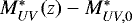 function, as presented in the upper panel of Fig. A.1, where the
  is the characteristic luminosity for galaxies at z = 0. Then the best-fitting exponential function in form,
 (A.1)
(A.1)
 |
Fig. A.1 Compilation of the values of Schechter characteristic UV
galaxy luminosity |
was used to normalize the absolute magnitudes of galaxies used in this paper. For each galaxy we take  , where
  is the original (not corrected) absolute magnitude.
We proceeded similarly to normalize the galaxy stellar masses. We took the characteristic stellar masses measured by Ilbert et al. (2013) and Pérez-González et al. (2008) in the redshift range 0 < z < 4 and fitted it with a simple exponential function, as presented in the lower panel of Fig. A.1. As before, the resulting best-fitting function,
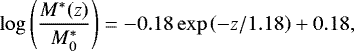 (A.2)
(A.2)
was used to normalize all stellar masses of the galaxies used in this study.
Appendix B Tests of sample variation – a large structure in the COSMOS field at z ~ 3
The correlation function measurements presented in this work were obtained from three independent VUDS fields (COSMOS, VVDS-02h, and ECDFS). The differences between these fields, such as their angular size and number of galaxies, are accounted for using an appropriate weighting scheme (see Sect. 3). This weighting scheme favours the biggest and the most populated fields to retrieve the best correlation function signal for all separations rp . At the same time, the differences between the correlation functions measured for the different fields yield information about the cosmic variance.
As a representative example in Fig. B.1 we show a comparison of the independent correlation function measurements for the MUV > −19.0 galaxy sample from two VUDS fields: COSMOS (red filled circles) and VVDS-02h (open blue circles). We note that in the further discussion we neglect the ECDFS field. Because its small size (Seff = 0.11 deg2), the measurement of the correlation function in this field does not contribute to the final wp (rp) measurement at scales rp > 5 h−1 Mpc on which the discussion below is focussed.
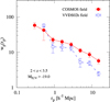 |
Fig. B.1 Projected two-point correlation function wp(rp) measured independently for the MUV > −19.0 galaxies in two VUDS fields. Red filled circles represent the correlation function measurements for the COSMOS field galaxy sample, while open blue circles show similar measurements for the VVDS-02h field sample. |
The most significant cosmic variance effect appears at large separations rp > 5 h−1 Mpc. At these large scales we observe a significant difference between the two correlation function measurements, as presented in Fig. B.1. The values of wp(rp) measured atrp > 5 h−1 Mpc for theCOSMOS field are approximately two times higher than the correlation function signal obtained for the VVDS-02h field. Naturally, this difference has an impact on the overall composite correlation function measurements presented in this work. The COSMOS field contains of the largest number of galaxies spread across the biggest effective surface (see Table 1). Therefore, the clustering results obtained for this field have the biggest impact on the final composite correlation function measurements, and this results in the higher values of the correlation function with respect to the best HOD models seen in Fig. 6. For all UV absolute magnitude and stellar mass selected subsamples, the correlation function measurement, at scales rp > 5 h−1 Mpc, is higher on average by a factor of 1.7 with respect to the HOD model.
The flattening of the correlation function measured in the COSMOS field at large scales is likely related to the existence of an extremely large structure of galaxies, possibly a proto-supercluster or a massive filament, at z ~ 2.5, which spans a size comparable to the entire filed covered by VUDS-COSMOS (Cucciati et al., in prep.). This would be the first observation of such a structure at high redshift. This hypothesis requires further investigation and is addressed in the dedicated follow-up research.
Ideally, to get the most robust measurements of the correlation function, one would exclude members of this structure from the measurements, however, firstly, the members of this structure have not been fully identified yet, and secondly, this would significantly lower the sample statistic and probably make it impossible to perform correlation function measurements for the luminosity and stellar mass selected galaxy samples.
References
- Abbas, U., de la Torre, S., Le Fèvre, O., et al. 2010, MNRAS, 406, 1306 [NASA ADS] [Google Scholar]
- Adelberger, K. L., Steidel, C. C., Pettini, M., et al. 2005, ApJ, 619, 697 [NASA ADS] [CrossRef] [Google Scholar]
- Arnouts, S., Cristiani, S., Moscardini, L., et al. 1999, MNRAS, 310, 540 [NASA ADS] [CrossRef] [Google Scholar]
- Bardeen, J. M., Bond, J. R., Kaiser, N., & Szalay, A. S. 1986, ApJ, 304, 15 [NASA ADS] [CrossRef] [Google Scholar]
- Barrow, J. D., Bhavsar, S. P., & Sonoda, D. H. 1984, MNRAS, 210, 19P [NASA ADS] [CrossRef] [Google Scholar]
- Behroozi, P. S., Conroy, C., & Wechsler, R. H. 2010, ApJ, 717, 379 [NASA ADS] [CrossRef] [Google Scholar]
- Behroozi, P. S., Wechsler, R. H., & Conroy, C. 2013, ApJ, 770, 57 [NASA ADS] [CrossRef] [Google Scholar]
- Benson, A. J., Frenk, C. S., Baugh, C. M., Cole, S., & Lacey, C. G. 2001, MNRAS, 327, 1041 [NASA ADS] [CrossRef] [Google Scholar]
- Beutler, F., Blake, C., Colless, M., et al. 2013, MNRAS, 429, 3604 [NASA ADS] [CrossRef] [Google Scholar]
- Bielby, R. M., Gonzalez-Perez, V., McCracken, H. J., et al. 2014, A&A, 568, A24 [NASA ADS] [CrossRef] [EDP Sciences] [Google Scholar]
- Blandford, R. D., & Narayan, R. 1992, ARA&A, 30, 311 [NASA ADS] [CrossRef] [Google Scholar]
- Blanton, M., Cen, R., Ostriker, J. P., & Strauss, M. A. 1999, ApJ, 522, 590 [NASA ADS] [CrossRef] [Google Scholar]
- Bouwens, R. J., & Illingworth, G. D. 2007, in Deepest Astronomical Surveys, eds. J. Afonso, H. C. Ferguson, B. Mobasher, & R. Norris, ASP Conf. Ser., 380, 41 [Google Scholar]
- Bouwens, R. J., Illingworth, G. D., Oesch, P. A., et al. 2015, ApJ, 803, 34 [NASA ADS] [CrossRef] [Google Scholar]
- Boylan-Kolchin, M., Bullock, J. S., & Kaplinghat, M. 2012, MNRAS, 422, 1203 [NASA ADS] [CrossRef] [Google Scholar]
- Brook, C. B., Di Cintio, A., Knebe, A., et al. 2014, ApJ, 784, L14 [NASA ADS] [CrossRef] [Google Scholar]
- Cassata, P., Le Fèvre, O., Charlot, S., et al. 2013, A&A, 556, A68 [NASA ADS] [CrossRef] [EDP Sciences] [Google Scholar]
- Chen, J., Bryan, G. L., & Salem, M. 2016, MNRAS, 460, 3335 [Google Scholar]
- Chiang, Y.-K., Overzier, R., & Gebhardt, K. 2013, ApJ, 779, 127 [NASA ADS] [CrossRef] [Google Scholar]
- Coil, A. L., Newman, J. A., Cooper, M. C., et al. 2006, ApJ, 644, 671 [NASA ADS] [CrossRef] [Google Scholar]
- Coil, A. L., Newman, J. A., Croton, D., et al. 2008, ApJ, 672, 153 [NASA ADS] [CrossRef] [Google Scholar]
- Conroy, C., Wechsler, R. H., & Kravtsov, A. V. 2006, ApJ, 647, 201 [NASA ADS] [CrossRef] [Google Scholar]
- Conselice, C. J., Rajgor, S., & Myers, R. 2008, MNRAS, 386, 909 [NASA ADS] [CrossRef] [Google Scholar]
- Coupon, J., Kilbinger, M., McCracken, H. J., et al. 2012, A&A, 542, A5 [NASA ADS] [CrossRef] [EDP Sciences] [Google Scholar]
- Daddi, E., Röttgering, H. J. A., Labbé, I., et al. 2003, ApJ, 588, 50 [NASA ADS] [CrossRef] [Google Scholar]
- Davis, M., & Peebles, P. J. E. 1983, ApJ, 267, 465 [NASA ADS] [CrossRef] [Google Scholar]
- de la Torre, S., Le Fèvre, O., Arnouts, S., et al. 2007, A&A, 475, 443 [NASA ADS] [CrossRef] [EDP Sciences] [Google Scholar]
- de la Torre, S., Guzzo, L., Peacock, J. A., et al. 2013, A&A, 557, A54 [NASA ADS] [CrossRef] [EDP Sciences] [Google Scholar]
- De Lucia, G., Springel, V., White, S. D. M., Croton, D., & Kauffmann, G. 2006, MNRAS, 366, 499 [NASA ADS] [CrossRef] [Google Scholar]
- De Lucia, G., Poggianti, B. M., Aragón-Salamanca, A., et al. 2007, MNRAS, 374, 809 [NASA ADS] [CrossRef] [Google Scholar]
- de Ravel, L., Le Fèvre, O., Tresse, L., et al. 2009, A&A, 498, 379 [NASA ADS] [CrossRef] [EDP Sciences] [Google Scholar]
- Dekel, A., Ishai, G., Dutton, A. A., & Maccio, A. V. 2017, MNRAS, 468, 1005 [NASA ADS] [CrossRef] [Google Scholar]
- Di Cintio, A., Brook, C. B., Macciò, A. V., et al. 2014, MNRAS, 437, 415 [NASA ADS] [CrossRef] [Google Scholar]
- Durkalec, A., Le Fèvre, O., de la Torre, S., et al. 2015a, A&A, 576, L7 [NASA ADS] [CrossRef] [EDP Sciences] [Google Scholar]
- Durkalec, A., Le Fèvre, O., Pollo, A., et al. 2015b, A&A, 583, A128 [Google Scholar]
- Erb, D. K. 2015, Nature, 523, 169 [NASA ADS] [CrossRef] [Google Scholar]
- Ferrara, A., & Tolstoy, E. 2000, MNRAS, 313, 291 [NASA ADS] [CrossRef] [Google Scholar]
- Ferrero, I., Abadi, M. G., Navarro, J. F., Sales, L. V., & Gurovich, S. 2012, MNRAS, 425, 2817 [Google Scholar]
- Finkelstein, S. L., Ryan, R. E., Jr., Papovich, C., et al. 2015, ApJ, 810, 71 [NASA ADS] [CrossRef] [Google Scholar]
- Fontanot, F., De Lucia, G., Monaco, P., Somerville, R. S., & Santini, P. 2009, MNRAS, 397, 1776 [NASA ADS] [CrossRef] [Google Scholar]
- Fry, J. N. 1996, ApJ, 461, L65 [NASA ADS] [CrossRef] [Google Scholar]
- Fu, L., Semboloni, E., Hoekstra, H., et al. 2008, A&A, 479, 9 [NASA ADS] [CrossRef] [EDP Sciences] [Google Scholar]
- Fujita, A., Mac Low, M.-M., Ferrara, A., & Meiksin, A. 2004, ApJ, 613, 159 [NASA ADS] [CrossRef] [Google Scholar]
- Garilli, B., Fumana, M., Franzetti, P., et al. 2010, PASP, 122, 827 [NASA ADS] [CrossRef] [Google Scholar]
- Genzel, R., Schreiber, N. M. F., Übler, H., et al. 2017, Nature, 543, 397 [NASA ADS] [CrossRef] [Google Scholar]
- Guo, H., Zheng, Z., Zehavi, I., et al. 2015, MNRAS, 453, 4368 [NASA ADS] [CrossRef] [Google Scholar]
- Guzzo, L., Strauss, M. A., Fisher, K. B., Giovanelli, R., & Haynes, M. P. 1997, ApJ, 489, 37 [NASA ADS] [CrossRef] [Google Scholar]
- Hagen, L. M. Z., Hoversten, E. A., Gronwall, C., et al. 2015, ApJ, 808, 178 [NASA ADS] [CrossRef] [Google Scholar]
- Hartley, W. G., Almaini, O., Cirasuolo, M., et al. 2010, MNRAS, 407, 1212 [NASA ADS] [CrossRef] [Google Scholar]
- Hatfield, P. W., Lindsay, S. N., Jarvis, M. J., et al. 2016, MNRAS, 459, 2618 [NASA ADS] [CrossRef] [Google Scholar]
- Hathi, N. P., Ryan, R. E., Jr., Cohen, S. H., et al. 2010, ApJ, 720, 1708 [NASA ADS] [CrossRef] [Google Scholar]
- Hildebrandt, H., Pielorz, J., Erben, T., et al. 2009, A&A, 498, 725 [NASA ADS] [CrossRef] [EDP Sciences] [Google Scholar]
- Hoekstra, H., Yee, H. K. C., & Gladders, M. D. 2004, ApJ, 606, 67 [NASA ADS] [CrossRef] [Google Scholar]
- Ilbert, O., Tresse, L., Zucca, E., et al. 2005, A&A, 439, 863 [NASA ADS] [CrossRef] [EDP Sciences] [Google Scholar]
- Ilbert, O., Arnouts, S., McCracken, H. J., et al. 2006, A&A, 457, 841 [NASA ADS] [CrossRef] [EDP Sciences] [Google Scholar]
- Ilbert, O., McCracken, H. J., Le Fèvre, O., et al. 2013, A&A, 556, A55 [NASA ADS] [CrossRef] [EDP Sciences] [Google Scholar]
- Ishikawa, S., Kashikawa, N., Toshikawa, J., et al. 2017, ApJ, 841, 8 [NASA ADS] [CrossRef] [Google Scholar]
- Jenkins, A., Frenk, C. S., White, S. D. M., et al. 2001, MNRAS, 321, 372 [NASA ADS] [CrossRef] [MathSciNet] [Google Scholar]
- Jones, O. C., Kemper, F., Sargent, B. A., et al. 2012, MNRAS, 427, 3209 [NASA ADS] [CrossRef] [Google Scholar]
- Kaiser, N. 1984, ApJ, 284, L9 [NASA ADS] [CrossRef] [Google Scholar]
- Katz, H., Lelli, F., McGaugh, S. S., et al. 2017, MNRAS, 466, 1648 [NASA ADS] [CrossRef] [Google Scholar]
- Kauffmann, G., Nusser, A., & Steinmetz, M. 1997, MNRAS, 286, 795 [NASA ADS] [CrossRef] [Google Scholar]
- Kawata, D., Gibson, B. K., Barnes, D. J., Grand, R. J. J., & Rahimi, A. 2014, MNRAS, 438, 1208 [NASA ADS] [CrossRef] [Google Scholar]
- Kilbinger, M., Benabed, K., Cappe, O., et al. 2011, ArXiv e-prints [arXiv:1101.0950] [Google Scholar]
- Landy, S. D., & Szalay, A. S. 1993, ApJ, 412, 64 [NASA ADS] [CrossRef] [Google Scholar]
- Le Fèvre, O., Guzzo, L., Meneux, B., et al. 2005, A&A, 439, 877 [NASA ADS] [CrossRef] [EDP Sciences] [Google Scholar]
- Le Fèvre, O., Tasca, L. A. M., Cassata, P., et al. 2015, A&A, 576, A79 [NASA ADS] [CrossRef] [EDP Sciences] [Google Scholar]
- Le Fèvre, O., Lemaux, B. C., Nakajima, K., et al. 2017, A&A, submitted [arXiv:1710.10715] [Google Scholar]
- Leauthaud, A., Tinker, J., Bundy, K., et al. 2012, ApJ, 744, 159 [NASA ADS] [CrossRef] [Google Scholar]
- Lee, K.-S., Giavalisco, M., Gnedin, O. Y., et al. 2006, ApJ, 642, 63 [NASA ADS] [CrossRef] [Google Scholar]
- Lilly, S. J., Le Fevre, O., Hammer, F., & Crampton, D. 1996, ApJ, 460, L1 [NASA ADS] [CrossRef] [Google Scholar]
- Lin, L., Dickinson, M., Jian, H.-Y., et al. 2012, ApJ, 756, 71 [NASA ADS] [CrossRef] [Google Scholar]
- López-Sanjuan, C., Le Fèvre, O., de Ravel, L., et al. 2011, A&A, 530, A20 [NASA ADS] [CrossRef] [EDP Sciences] [Google Scholar]
- López-Sanjuan, C., Le Fèvre, O., Tasca, L. A. M., et al. 2013, A&A, 553, A78 [NASA ADS] [CrossRef] [EDP Sciences] [Google Scholar]
- Magliocchetti, M., & Porciani, C. 2003, MNRAS, 346, 186 [NASA ADS] [CrossRef] [Google Scholar]
- Marulli, F., Bolzonella, M., Branchini, E., et al. 2013, A&A, 557, A17 [NASA ADS] [CrossRef] [EDP Sciences] [Google Scholar]
- Mashchenko, S., Wadsley, J., & Couchman, H. M. P. 2008, Science, 319, 174 [NASA ADS] [CrossRef] [Google Scholar]
- Mason, C. A., Trenti, M., & Treu, T. 2015, ApJ, 813, 21 [NASA ADS] [CrossRef] [Google Scholar]
- Massey, R., Rhodes, J., Ellis, R., et al. 2007, Nature, 445, 286 [NASA ADS] [CrossRef] [PubMed] [Google Scholar]
- McCracken, H. J., Wolk, M., Colombi, S., et al. 2015, MNRAS, 449, 901 [NASA ADS] [CrossRef] [Google Scholar]
- McLure, R. J., Dunlop, J. S., Bowler, R. A. A., et al. 2013, MNRAS, 432, 2696 [NASA ADS] [CrossRef] [Google Scholar]
- Meneux, B., Le Fèvre, O., Guzzo, L., et al. 2006, A&A, 452, 387 [NASA ADS] [CrossRef] [EDP Sciences] [Google Scholar]
- Meneux, B., Guzzo, L., Garilli, B., et al. 2008, A&A, 478, 299 [NASA ADS] [CrossRef] [EDP Sciences] [Google Scholar]
- Meneux, B., Guzzo, L., de la Torre, S., et al. 2009, A&A, 505, 463 [NASA ADS] [CrossRef] [EDP Sciences] [Google Scholar]
- Metcalf, R. B., & Madau, P. 2001, ApJ, 563, 9 [NASA ADS] [CrossRef] [Google Scholar]
- Meylan, G., Jetzer, P., North, P., et al., eds. 2006, Gravitational Lensing: Strong, Weak and Micro (Berlin: Springer) [Google Scholar]
- Miller, S. H., Ellis, R. S., Newman, A. B., & Benson, A. 2014, ApJ, 782, 115 [NASA ADS] [CrossRef] [Google Scholar]
- Mo, H. J., & White, S. D. M. 1996, MNRAS, 282, 347 [NASA ADS] [CrossRef] [Google Scholar]
- Mostek, N., Coil, A. L., Cooper, M., et al. 2013, ApJ, 767, 89 [NASA ADS] [CrossRef] [Google Scholar]
- Moster, B. P., Naab, T., & White, S. D. M. 2013, MNRAS, 428, 3121 [NASA ADS] [CrossRef] [Google Scholar]
- Moustakas, L. A., & Metcalf, R. B. 2003, MNRAS, 339, 607 [NASA ADS] [CrossRef] [Google Scholar]
- Newman, S. F., Genzel, R., Förster-Schreiber, N. M., et al. 2012, ApJ, 761, 43 [NASA ADS] [CrossRef] [Google Scholar]
- Norberg, P., Baugh, C. M., Hawkins, E., et al. 2002, MNRAS, 332, 827 [NASA ADS] [CrossRef] [Google Scholar]
- Oñorbe, J., Boylan-Kolchin, M., Bullock, J. S., et al. 2015, MNRAS, 454, 2092 [NASA ADS] [CrossRef] [Google Scholar]
- Ogiya, G., & Mori, M. 2014, ApJ, 793, 46 [NASA ADS] [CrossRef] [Google Scholar]
- Ouchi, M., Hamana, T., Shimasaku, K., et al. 2005, ApJ, 635, L117 [NASA ADS] [CrossRef] [Google Scholar]
- Papastergis, E., & Shankar, F. 2016, A&A, 591, A58 [NASA ADS] [CrossRef] [EDP Sciences] [Google Scholar]
- Parsa, S., Dunlop, J. S., McLure, R. J., & Mortlock, A. 2016, MNRAS, 456, 3194 [Google Scholar]
- Peacock, J. A., & Smith, R. E. 2000, MNRAS, 318, 1144 [NASA ADS] [CrossRef] [Google Scholar]
- Peebles, P. J. E. 1980, The Large-Scale Structure of the Universe (Princeton, NJ: Princeton University Press) [Google Scholar]
- Pérez-González, P. G., Rieke, G. H., Villar, V., et al. 2008, ApJ, 675, 234 [NASA ADS] [CrossRef] [Google Scholar]
- Pettini, M., Shapley, A. E., Steidel, C. C., et al. 2001, ApJ, 554, 981 [NASA ADS] [CrossRef] [Google Scholar]
- Planck Collaboration XVI. 2014, A&A, 571, A16 [NASA ADS] [CrossRef] [EDP Sciences] [Google Scholar]
- Pollo, A., Meneux, B., Guzzo, L., et al. 2005, A&A, 439, 887 [NASA ADS] [CrossRef] [EDP Sciences] [Google Scholar]
- Pollo, A., Guzzo, L., Le Fèvre, O., et al. 2006, A&A, 451, 409 [NASA ADS] [CrossRef] [EDP Sciences] [Google Scholar]
- Pontzen, A., & Governato, F. 2012, MNRAS, 421, 3464 [NASA ADS] [CrossRef] [Google Scholar]
- Press, W. H., & Schechter, P. 1974, ApJ, 187, 425 [NASA ADS] [CrossRef] [Google Scholar]
- Read, J. I., Iorio, G., Agertz, O., & Fraternali, F. 2017, MNRAS, 467, 2019 [NASA ADS] [Google Scholar]
- Reddy, N. A., & Steidel, C. C. 2009, ApJ, 692, 778 [NASA ADS] [CrossRef] [Google Scholar]
- Rines, K., Geller, M. J., Diaferio, A., & Kurtz, M. J. 2013, ApJ, 767, 15 [NASA ADS] [CrossRef] [Google Scholar]
- Robertson, B. E. 2010, ApJ, 713, 1266 [NASA ADS] [CrossRef] [Google Scholar]
- Rubin, V. C., Thonnard, N., & Ford, W. K., Jr. 1978, ApJ, 225, L107 [NASA ADS] [CrossRef] [Google Scholar]
- Sawala, T., Guo, Q., Scannapieco, C., Jenkins, A., & White, S. 2011, MNRAS, 413, 659 [NASA ADS] [CrossRef] [Google Scholar]
- Sawala, T., Frenk, C. S., Crain, R. A., et al. 2013, MNRAS, 431, 1366 [NASA ADS] [CrossRef] [Google Scholar]
- Sawala, T., Frenk, C. S., Fattahi, A., et al. 2015, MNRAS, 448, 2941 [NASA ADS] [CrossRef] [Google Scholar]
- Sawicki, M., & Thompson, D. 2006, ApJ, 648, 299 [NASA ADS] [CrossRef] [Google Scholar]
- Schechter, P. 1976, ApJ, 203, 297 [Google Scholar]
- Seljak, U. 2000, MNRAS, 318, 203 [NASA ADS] [CrossRef] [Google Scholar]
- Shapley, A. E., Steidel, C. C., Pettini, M., & Adelberger, K. L. 2003, ApJ, 588, 65 [NASA ADS] [CrossRef] [Google Scholar]
- Sheth, R. K., Mo, H. J., & Tormen, G. 2001, MNRAS, 323, 1 [NASA ADS] [CrossRef] [Google Scholar]
- Skibba, R. A., Coil, A. L., Mendez, A. J., et al. 2015, ApJ, 807, 152 [NASA ADS] [CrossRef] [Google Scholar]
- Springel, V., White, S. D. M., Jenkins, A., et al. 2005, Nature, 435, 629 [NASA ADS] [CrossRef] [PubMed] [Google Scholar]
- Steidel, C. C., Erb, D. K., Shapley, A. E., et al. 2010, ApJ, 717, 289 [NASA ADS] [CrossRef] [Google Scholar]
- Talia, M., Brusa, M., Cimatti, A., et al. 2017, MNRAS, 471, 4527 [NASA ADS] [CrossRef] [Google Scholar]
- Tasca, L. A. M., Le Fèvre, O., López-Sanjuan, C., et al. 2014, A&A, 565, A10 [NASA ADS] [CrossRef] [EDP Sciences] [Google Scholar]
- Tasca, L. A. M., Le Fèvre, O., Hathi, N. P., et al. 2015, A&A, 581, A54 [NASA ADS] [CrossRef] [EDP Sciences] [Google Scholar]
- Tegmark, M., & Peebles, P. J. E. 1998, ApJ, 500, L79 [NASA ADS] [CrossRef] [Google Scholar]
- Tegmark, M., Blanton, M. R., Strauss, M. A., et al. 2004, ApJ, 606, 702 [NASA ADS] [CrossRef] [Google Scholar]
- Thomas, R., Le Fèvre, O., Scodeggio, M., et al. 2017, A&A, 602, A35 [NASA ADS] [CrossRef] [EDP Sciences] [Google Scholar]
- Van Waerbeke, L., Mellier, Y., Erben, T., et al. 2000, A&A, 358, 30 [NASA ADS] [Google Scholar]
- Wake, D. A., Whitaker, K. E., Labbé, I., et al. 2011, ApJ, 728, 46 [NASA ADS] [CrossRef] [Google Scholar]
- Wang, L., Li, C., Kauffmann, G., & De Lucia, G. 2007, MNRAS, 377, 1419 [NASA ADS] [CrossRef] [Google Scholar]
- Weiner, B. J., Coil, A. L., Prochaska, J. X., et al. 2009, ApJ, 692, 187 [NASA ADS] [CrossRef] [Google Scholar]
- Weinmann, S. M., Pasquali, A., Oppenheimer, B. D., et al. 2012, MNRAS, 426, 2797 [NASA ADS] [CrossRef] [Google Scholar]
- Wetzel, A. R., Cohn, J. D., & White, M. 2009, MNRAS, 395, 1376 [NASA ADS] [CrossRef] [Google Scholar]
- White, S. D. M. 1976, MNRAS, 177, 717 [NASA ADS] [CrossRef] [Google Scholar]
- White, S. D. M., & Rees, M. J. 1978, MNRAS, 183, 341 [NASA ADS] [CrossRef] [Google Scholar]
- White, S. D. M., Davis, M., Efstathiou, G., & Frenk, C. S. 1987, Nature, 330, 451 [NASA ADS] [CrossRef] [Google Scholar]
- Wraith, D., Kilbinger, M., Benabed, K., et al. 2009, Phys. Rev. D, 80, 023507 [NASA ADS] [CrossRef] [Google Scholar]
- Yang, X., Mo, H. J., van den Bosch, F. C., Zhang, Y., & Han, J. 2012, ApJ, 752, 41 [NASA ADS] [CrossRef] [Google Scholar]
- Zehavi, I., Weinberg, D. H., Zheng, Z., et al. 2004, ApJ, 608, 16 [NASA ADS] [CrossRef] [Google Scholar]
- Zehavi, I., Zheng, Z., Weinberg, D. H., et al. 2011, ApJ, 736, 59 [NASA ADS] [CrossRef] [Google Scholar]
- Zheng, Z., Berlind, A. A., Weinberg, D. H., et al. 2005, ApJ, 633, 791 [NASA ADS] [CrossRef] [Google Scholar]
- Zheng, Z., Coil, A. L., & Zehavi, I. 2007, ApJ, 667, 760 [NASA ADS] [CrossRef] [Google Scholar]
- Zwicky, F. 1937, ApJ, 86, 217 [NASA ADS] [CrossRef] [Google Scholar]
M⋆ = 109.1 M⊙ in Durkalec et al. (2015a), M⋆ = 109.4 M⊙ in Ishikawa et al. (2017) and M⋆ = 1010 M⊙ in McCracken et al. (2015).
All Tables
All Figures
|
Fig. 1 Spatial distribution of galaxies with spectroscopic redshifts 2 < z < 3.5 in three independent VUDS fields: COSMOS (left panel), VVDS-02h (central panel), and ECDFS (right panel). The blue crosses indicate VIMOS pointing centres. |
| In the text | |
|
Fig. 2 Redshift distribution of the VUDS galaxy sample in the redshift range 2.0 < z < 3.5 used in this study. The filled grey histogram represents the total sample of galaxies, while the red, blue, and green histograms represent the contribution from COSMOS, VVDS-02h, and ECDFS fields, respectively. |
| In the text | |
|
Fig. 3 Construction of the volume-limited galaxy subsamples with different luminosity
(upper panel) and stellar mass (lower panel). In both figures the grey dots
represent the distribution of VUDS galaxies as a function of spectroscopic redshift
z.
At each redshift UV
band, absolute magnitudes and stellar masses are normalized to the characteristic absolute magnitudes or to the
characteristic stellar mass, respectively (see Sect. 2.2). The different colour lines delineate the selection cuts
for selected UV
absolute magnitude and stellar mass subsamples as defined in Tables 2 and
3. The dashed black line represents the evolution of the not corrected characteristic
UV
absolute magnitude |
| In the text | |
|
Fig. 4 Projected correlation functions for volume-limited samples corresponding to different luminosity (left panel, circles) and stellar mass (right panel, squares) bins, as labelled. |
| In the text | |
|
Fig. 5 Projected two-point correlation function wp(rp) associated with the best-fitting power-law function (left side) and best-fit power-law parameters r0 and γ along with 68.3% and 95.4% joint confidence levels (right side) in four UV absolute magnitude subsamples (upper panel) and four stellar mass subsamples (lower panel). The symbols and error bars (see Sect. 3 for the error estimation method) denote measurements of the composite correlation function for different luminosity (circles) and stellar mass (squares) subsamples selected from VUDS survey in the redshift range 2 < z < 3.5. For clarity, offsets are applied both to the data points and best-fitting curves of the wp (rp), i.e. the values of wp(rp) and associated best fits for galaxy subsamples with increasing luminosity and stellar masses were staggered by 0.5 dex each. Error contours on the fit parameters are obtained taking into account the full covariance matrix. The 68.3% and 95.4% joint confidence levels are defined in terms of the corresponding likelihood intervals that we obtain from our fitting procedure. |
| In the text | |
|
Fig. 6 Projected two-point correlation function wp(rp) associated with the best-fitting HOD models (left side) and evolution of the halo occupation function of the best-fit HOD model (right side) in four UV absolute magnitude subsamples (upper panel) and four stellar mass subsamples (lower panel). The symbols and error bars (see Sect. 3 for the error estimation method) denote measurements of the composite correlation function for different luminosity (circles) and stellar mass (squares) subsamples selected from the VUDS survey in the redshift range 2 < z < 3.5. For clarity, offsets are applied to both the data points and best-fitting curves of the wp (rp), i.e. the values of wp(rp) and associated best fits for the galaxy subsamples with increasing luminosity and stellar masses were staggered by 0.5 dex each. |
| In the text | |
|
Fig. 7 Relative bias b∕b* (see Eq. (12)) for the selected VUDS luminosity subsamples at z ~ 3 (orange circles) as a function of luminosity with L* as a reference point. The results from this work are compared to similar studies at lower redshift ranges: at z ~ 0.1 from Zehavi et al. (2011) (filled black circles) and Norberg et al. (2002) (black crosses), and at z ~ 0.9 from Pollo et al. (2006) (green circles). The lines indicate the analytic fit of the 2dFGRS data from Norberg et al. (2002) (black solid line) and SDSS data from Tegmark et al. (2004) (black dashed line), as described in the text. |
| In the text | |
|
Fig. 8 Large-scale galaxy bias bg,HOD as a functionof luminosity, with L* as a reference point (left panel) and as a function of stellar mass with M* as a reference point (right panel). In both plots, the coloured points indicate measurements at z ~ 3 from this work; the solid lines indicate the best-fit functions of the bias-luminosity dependence bg,HOD(>L) (Eq. (13)) and bias-stellar mass dependence bg,HOD(>M) (Eq. (14)) as described in Sect. 5.2. In the left panel, the black circles show the results from Zehavi et al. (2011) at z ~ 0 and the dashed line represents the empirical fit of the bias-luminosity dependence in the functional form given therein. In the right panel, we show for comparison the bg measurements at z ~ 0.5 from Skibba et al. (2015) represented by open circles, those at z ~ 1 by Mostek et al. (2013) are indicated by black triangles and from different samples in the redshift range 0.5 < z < 2.5 measured by McCracken et al. (2015) shown as black lines as labelled. |
| In the text | |
|
Fig. 9 Characteristic halo masses from the best-fitting HOD models of the correlation function selected in luminosity vs. Lthresh∕L* (left panel) and selected in stellar mass vs. Mthresh∕M* (right panel). Minimum halo masses Mmin for which 50% of haloes host one central galaxy above the threshold limit (filled symbols) and masses of haloes which on average host one additional satellite galaxy M1 (open symbols) observed at z ~ 3 are compared with similar results found by Zehavi et al. (2011) at z ~ 0, for the luminosity selected galaxies, and by Skibba et al. (2015) at z ~ 0.5, for the stellar mass selected galaxies (dotted and dashed lines). |
| In the text | |
|
Fig. 10 Satellite fraction fs as a functionof threshold luminosity, with L* as a reference point (left panel) and as a function of threshold stellar mass, with M* as a reference point (right panel). Results obtained in this work at z ~ 3 (filled symbols) are compared with similar measurements from lower redshift ranges. In the left panel the dashed line indicates the satellite fraction as measured at z ~ 0 by Zehavi et al. (2011), while in the right panel results found by Skibba et al. (2015) at z ~ 0.5 are shown with open triangles. |
| In the text | |
|
Fig. 11 Stellar mass–halo mass relation (SHMR) of central galaxies obtained for different stellar mass selected subsamples
at z ~ 3
(orange symbols). The halo masses are represented by the best-fit parameter
Mmin ,
while the associated stellar masses of the galaxies are represented by the threshold limits
|
| In the text | |
|
Fig. A.1 Compilation of the values of Schechter characteristic UV
galaxy luminosity |
| In the text | |
|
Fig. B.1 Projected two-point correlation function wp(rp) measured independently for the MUV > −19.0 galaxies in two VUDS fields. Red filled circles represent the correlation function measurements for the COSMOS field galaxy sample, while open blue circles show similar measurements for the VVDS-02h field sample. |
| In the text | |
Current usage metrics show cumulative count of Article Views (full-text article views including HTML views, PDF and ePub downloads, according to the available data) and Abstracts Views on Vision4Press platform.
Data correspond to usage on the plateform after 2015. The current usage metrics is available 48-96 hours after online publication and is updated daily on week days.
Initial download of the metrics may take a while.