| Issue |
A&A
Volume 610, February 2018
|
|
|---|---|---|
| Article Number | A64 | |
| Number of page(s) | 14 | |
| Section | Galactic structure, stellar clusters and populations | |
| DOI | https://doi.org/10.1051/0004-6361/201731153 | |
| Published online | 02 March 2018 | |
A revised estimate of the distance to the clouds in the Chamaeleon complex using the Tycho–Gaia Astrometric Solution★
Scientific Support Office, Directorate of Science, European Space Research and Technology Center (ESA/ESTEC),
Keplerlaan 1,
2201
AZ Noordwijk, The Netherlands
e-mail: This email address is being protected from spambots. You need JavaScript enabled to view it.
Received:
11
May
2017
Accepted:
11
October
2017
Abstract
Context. The determination of the distance to dark star-forming clouds is a key parameter to derive the properties of the cloud itself and of its stellar content. This parameter is still loosely constrained even in nearby star-forming regions.
Aim. We want to determine the distances to the clouds in the Chamaeleon-Musca complex and explore the connection between these clouds and the large-scale cloud structures in the Galaxy.
Methods. We used the newly estimated distances obtained from the parallaxes measured by the Gaia satellite and included in the Tycho–Gaia Astrometric Solution catalog. When known members of a region are included in this catalog we used their distances to infer the distance to the cloud. Otherwise, we analyzed the dependence of the color excess on the distance of the stars and looked for a turn-on of this excess, which is a proxy of the position of the front-edge of the star-forming cloud.
Results. We are able to measure the distance to the three Chamaeleon clouds. The distance to Chamaeleon I is 179-10-10+11+11pc, where the quoted uncertainties are statistical and systematic uncertainties, respectively, ~20 pc further away than previously assumed. The Chamaeleon II cloud is located at the distance of 181-5-10+6+11pc, which agrees with previous estimates. We are able to measure for the first time a distance to the Chamaeleon III cloud of 199-7-11+8+12pc. Finally, the distance of the Musca cloud is smaller than 603603-70-92+91+133 pc. These estimates do not allow us to distinguish between the possibility that the Chamaeleon clouds are part of a sheet of clouds parallel to the Galactic plane, or perpendicular to it.
Conclusions. We measured a larger distance to the Chamaeleon I cloud than assumed in the past, confirmed the distance to the Chamaeleon II region, and measured for the first time the distance to the Chamaleon III cloud. These values are consistent with the scenario in which the three clouds are part of a single large-scale structure. Gaia Data Release 2 will allow us to put more stringent constraints on the distances to these clouds by giving us access to parallax measurements for a larger number of members of these regions.
Key words: stars: distances / stars: formation / dust, extinction / open clusters and associations: individual: Chamaeleon / ISM: clouds
Tables 3–6 are only available at the CDS via anonymous ftp to cdsarc.u-strasbg.fr (130.79.128.5) or via http://cdsarc.u-strasbg.fr/viz-bin/qcat?J/A+A/610/A64
ESA Research Fellow; Current address: European Southern Observatory, Karl-Schwarzschild-Str. 2, 85748 Garching bei München, Germany.
© ESO 2018
1 Introduction
Star-forming regions in the solar neighborhood are ideal laboratories to study pre-main-sequence (PMS) evolution and properties of star-forming clouds. One key parameter in these studies is the distance to the objects. Many physical properties, such as cloud size and mass, stellar luminosity, and space motion depend on distance. Any uncertainty in the distance estimate directly translates into uncertainty in the deduced age, mass, and other properties of young stellar objects (YSOs).
To date, the major limitation in the estimate of the distance to star-forming clouds is the lack of directly measured parallaxes for a large number of stars, which are mainly available from the HIPPARCOS parallaxes (Perryman et al. 1997) for the brightest nearby stars. Therefore, photometric determined distances have been used in the past (e.g., Whittet et al. 1997) to derive distances with relatively high uncertainties. The Gaia mission (Gaia Collaboration 2016b) is overcoming this limitation. In particular, the Tycho-Gaia Astrometric Solution (TGAS) from the first Gaia data release (Gaia Collaboration 2016a) already provides parallaxes to stars down to G ~ 12 mag. Data from TGAS can be used to determine distances both of members of a given star-forming cloud or to field stars in its vicinity. We use this information in this work to determine the distance to the nearby Chamaleon-Musca star-forming complex.
The proximity of the Chamaeleon-Musca star-forming complex has triggered many studies of the system and its PMS population. The complex contains four dark clouds: Chamaeleon I, II, III, and Musca (Luhman 2008). These objects are visible in the Gaia stellar density map shown in Fig. 1. The extinction of the central parts of the clouds is so high that very few stars can be seen through to the limiting magnitude G < 20.7 of Gaia. The complex is located southward of the Galactic plane around l = 300°, b = −15°.
The distance to the Chamaeleon I dark cloud has been extensively discussed in the literature. The previous results vary between 115 and 215 pc (Schwartz 1992). In Whittet et al. (1987), the analysis of the reddening of field stars along the line of sight led to a distance estimate of 140 ± 12 pc. In Franco (1991) the distance to the cloud is also found to be 140 pc. The latest result by Whittet et al. (1997) combined the method of reddening turn-on with other distance indicators and deduced 160 ± 15 pc. This is the commonly assumed distance to the stars in this region (e.g., Luhman 2008).
The distance to Chamaeleon II is more difficult to pin down and consequently less certain. Initially, this was constrained to be within 115 and 400 pc (Graham & Hartigan 1988). In Franco (1991) the analysis of the extinction distribution along the line of sight gave a distance of 158 ± 40 pc. Hughes & Hartigan (1992) deduced a distance of 200 ± 20 pc. In Whittet et al. (1997), the distance to the Chamaeleon II cloud was found to be 178 ± 18 pc.
For the Chamaeleon III dark cloud the distance is poorly constrained in the literature. Whittet et al. (1997) gives an estimate using the assumption that the Chamaeleon star-forming region is on a sheet of clouds parallel to the Galactic plane (as later discussed in Sect. 4.2). Using this assumption their estimate was 140–160 pc.
The Musca cloud is located northward of the Chamaeleon region (see Fig. 1). It is a thin elongated dark cloud possibly about to start forming stars (Cox et al. 2016). Its distance is not well constrained in the literature partly because no PMS stars have been identified at optical wavelengths in the cloud. Franco (1991) argues that it is part of the Chamaeleon system and thus should be around 140 pc.
The paper is structured in five sections. After the introduction, Sect. 2 presents the methods used to determine the distances to the clouds. In Sect. 3 results are given individually for each cloud. Section 4 addresses the question of the physical structure of the Chamaeleon-Musca complex and the impact on PMS properties of the newly deduced distances. Finally, in Sect. 5 we summarize our conclusions.
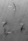 |
Fig. 1 Gaia star density map of the Chamaeleon-Musca region. The figure is a 11° × 13° field centered on the coordinates (l = 300.5°, b = −13.3°). |
2 Methods to determine cloud distances
Two different methods are used to determine the distances to the clouds in the Chamaeleon-Musca complex, and we describe both methods in this section.
2.1 Members distance
The distance to a single star may be unreliable as an indication of the distance to a cluster of young stars. Taking advantage of the fact that stars often form together and analyzing distances to all members of a cluster it is possible to have a more reliable estimate. Photometric distances to PMS stars are uncertain as standard colors, extinction, and luminosity are all poorly known. A more reliable way by far is to have a direct trigonometric measurement.
We selected PMS stars for which the parallax has been directly measured with Gaia. At this stage this is limited to the TGAS catalog (Gaia Collaboration 2016a). The trigonometric parallaxes have been converted to distances by assuming an anisotropic prior derived from the observed stars in a Milky Way model as discussed in Astraatmadja & Bailer-Jones (2016), using the values obtained without including the systematic uncertainties on the parallaxes. In the following we adopt the mode value of the inferred distances plus or minus the difference to the 5 and 95 percentile of the posteriors, following Bailer-Jones (2015). This implies that the uncertainties we quote on the TGAS distances correspond to a 2σ uncertainty.
The distance to a region determined using the distances to individual confirmed members is then taken as the inverse of the mean value of the parallax to the members, weighted for their squared 1σ uncertainty, following, for example, de Zeeuw et al. (1999).
2.2 Reddening turn-on distance
The second method is based on the principle that the presence of a cloud results in an sudden increase of the extinction at the distance of the front edge of the cloud. Using the measurements of field stars in the line of sight toward a cloud, it is possible to deduce a distance where the increase of the extinction happens. This method is particularly useful in the Chamaeleon complex, given its vicinity and apparent lack of material in front of the clouds (Whittet et al. 1997; Corradi et al. 1997). Indeed, this method has limitations if applied to non-homogeneous clouds, where a background star could be located on the line of sight of the cloud but observed at negligible extinction or in cases where significant extinction is present in front of the cloud.
We chose only stars for which the parallax has been directly measured with Gaia (Gaia Collaboration 2016b). We selected the stars spatially located in the line of sight to the clouds. The cloud extent is determined using the Infrared Astronomical Satellites (IRAS) 100 μm flux map1 (Schlegel et al. 1998).
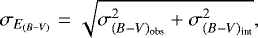
The B − V color excess (E(B−V )) caused by extinction, is given by the following formula:
 (1)
(1)
where  is the observed color of a star in the Johnson–Cousins system and
  is the intrinsic color in the Johnson–Cousins system.
The observed colors are computed from the Tycho 2 photometry in the BT and V T bands (H∅g et al. 2000) by transforming to the Johnson–Cousins system as discussed in Perryman et al. (1997). The intrinsic colors depend on the spectral type (SpT) and luminosity class of the star. Here, we used the relations between the spectral type and the intrinsic color by Gottlieb (1978) and Pecaut & Mamajek (2013). We used the compilation by Pecaut & Mamajek (2013) for dwarfs and subgiants with spectral type between K1 and M5, and that by Gottlieb (1978) for earlier type subgiants, giants, and stars with luminosity classes I and II. The consistency of the two catalogs is shown in Fig. 2. The difference between the two is in general small and always ≤0.1 mag for dwarfs and ≤0.15 mag for subgiants.
The spectral types for the stars in our sample are taken from the reference reported in Simbad (Wenger et al. 2000) and these are reported in Tables 3–6. When the luminosity class information is missing from Simbad, we determined it using a color magnitude diagram (CMD), as discussed in Appendix A. There are stars for which Simbad reports only the effective temperature (Teff )2. We determined their spectral type using the Teff-SpT relation corresponding to the luminosity class determined from the CMD. The Teff -SpT relations are taken from Pecaut & Mamajek (2013) for dwarfs and subgiants, while such relations for giant stars are a combination of Perrin et al. (1998) and Alonso et al. (1999).
The uncertainty on the color excess is computed using the following formula:
 (2)
(2)
where  is the uncertainty on color excess,
  is the uncertainty on the observed color, and
  is the uncertainty on the intrinsic color. The uncertainty on the observed color depends on the uncertainty of the Tycho-2 magnitude measurements
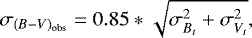 (3)
(3)
where  is the uncertainty on Bt magnitude,
  is the uncertainty on V t magnitude and the factor comes from the transformation between the instrumental magnitude system and the Johnson–Cousins system. The uncertainty on the intrinsic color is directly linked to the spectral type uncertainty. The latter is assumed to be of one subclass consistent with other work (Andersson et al. 2011; Torres et al. 2006). In the case of stars with only the effective temperature, its uncertainty comprises the uncertainty on the spectral type. For estimating the uncertainty on the intrinsic color the uncertainty of the spectral type is used.
The distance to the cloud is derived from the analysis of the extinction distribution along the line of sight toward field stars. The absorption due to the cloud material causes an increase of the color excess indicating the onset of extinction due to the cloud. The front edge of the cloud lies in the interval between the non-reddened field stars in front of the cloud and the reddened stars behind it. The distance to the cloud is defined as the inverse of the weighted mean parallax of the last non-reddened on-cloud star and the first reddened star. Practically, it means that the star in front of the edge of the cloud must have 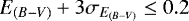 mag and the star after the edge must have a
  mag to be included in the analysis of the cloud distance. The choice of 0.2 mag is driven by the fact that our measurements on non-reddened stars lead to negative value of the colors as large as ~–0.2 mag, which is then considered as our systematic uncertainty.
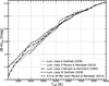 |
Fig. 2 Comparison of |

3 Results
We present the results for each cloud independently. For the Chamaeleon I cloud both analysis methods could be used, since eight of its confirmed members are included in the TGAS catalog. On the contrary, only the reddening turn-on method can be used to constrain the distance of the other clouds.
3.1 Chamaeleon I
3.1.1 Members analysis
The Chamaeleon I star-forming region comprises more than 200 members (Luhman 2004, 2007; Luhman & Muench 2008). We searched in the TGAS catalog (Gaia Collaboration 2016a) for members of this region and found that eight of the brightest objects are included. The limited number of matches is due to the magnitude limit (G ~12 mag) of the TGAS catalog. Five of these targets were already included in the HIPPARCOS catalog (van Leeuwen 2007). Their parallaxes and distances are reported in Table 1, obtained by inverting the parallax for the HIPPARCOS data and from Astraatmadja & Bailer-Jones (2016) for TGAS data, and including the errors on these values. While for parallaxes the 1σ uncertainty is reported, for distances wecomputed the 1σ asymmetric error on the HIPPARCOS distances from the inversion of the parallax plus or minus its error, and we reported the difference to the 5 and95 percentile of the median of the TGAS distance reported by Astraatmadja & Bailer-Jones (2016). The latter is a 2σ uncertainty. The comparison between the parallaxes and the corresponding inferred distances reported in the two catalogs is shown in Fig. 3. The new estimates of the parallaxes and their inferred distances to these five objects with TGAS are larger than the HIPPARCOS ones in four cases, although the two sets of values are compatible within their uncertainty.
The positions and proper motions vectors for the eight previously reported members are reported in Table 2 and shown in Fig. 4. These objects are located in different parts of the cloud, spanning from the dust cloudlet on the north end to the dust-depleted region to the south, and their individual distances range from ~160 pc to ~200 pc with typicaluncertainties of 8–9 pc. There is a hint of a north-south distance gradient, with the target TYC 9410-1954-1, located in the northern cloudlet, having a distance of 162 pc, stars in the dense region at the center having distances between ~180–190 pc, and the star on the southern part, TYC 9414-33-1 having a distance of 207
 pc. However, this could also indicate that the north cloudlet is separated from the main Chamaeleon I cloud, and lays ~20 pc closer to us,or even that the Chamaeleon I cloud is actually composed of three different regions. We are not yet in a position to discriminate between these hypotheses due to the still large uncertainties on the distances and to the limited number of targets. Therefore, we consider the objects in this cloud to be located at a single distance.
To determine the distance of the Chamaeleon I cloud based on the distances to its individual members we first note that two of these members have different proper motions and distances with respect to the other members. These are TYC 9414-33-1, which is located outside the cloud on the southern side at a distance of almost 210 pc, and TYC 9410-1954-1, which is at ~160 pc and in the northern cloudlet. The former is considered a member of Chamaelon I since it has a proper motion direction similar to other members of this region that are too faint to be in the TGAS catalog (Lopez Martí et al. 2013). We determine the distance to the Chamaeleon I cloud by performing a weighted mean over the parallaxes to the other six members, and we invert this mean parallax to obtain
![Mathematical equation: \begin{equation*} \bar{\textrm{d}}_{\textrm{Chamaeleon \ I, \ members}} = 188 ^{+6+11}_{-6-10} \ [\textrm{pc}],\end{equation*}](/articles/aa/full_html/2018/02/aa31153-17/aa31153-17-eq19.png) (4)
(4)
where the uncertainties are 1σ statistical and systematic3 uncertainties, respectively. This value would be  pc if TYC 9410-1954-1 is also included, and
  pc if all the eight members included in the TGAS catalog are considered. All these values are consistent within their statistical uncertainties and we thus use the value reported in Eq. (4) as a reference in the following.
HIPPARCOS and TGAS parallaxes and inferred distances of the five members of Chamaeleon I included in both catalogs.
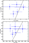 |
Fig. 3 Top: TGAS parallaxes (πTGAS) vs. HIPPARCOS parallaxes (πHip) to the five members of Chamaeleon I included in both HIPPARCOS catalog (van Leeuwen 2007) and TGAS catalog (Gaia Collaboration 2016a). The black line represents the one to one relation. Bottom: same for distances, taken as inverse of the parallax for HIPPARCOS data and from Astraatmadja & Bailer-Jones (2016) for TGAS (see Table 1). Uncertainties on both axes are as discussed in Table 1, and they correspond to 1σ uncertainty for the HIPPARCOS values and 2σ for TGAS. |
Members of Chamaeleon I included in the TGAS catalog.
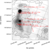 |
Fig. 4 IRAS maps of the Chamaeleon I region at 100 μm (Schlegel et al. 1998). The six contours range from 8 MJy/sr to 30 MJy/sr. The positions of the members of this region included in the TGAS catalog are represented with red circles. The red arrows represent their displacement in 105 yr. The Tycho-2 or HIPPARCOS name and TGAS distance of each star are reported as labels for each object. |
3.1.2 Reddening turn-on analysis
The reddening turn-on method described in Sect. 2.2 is used here to obtain a distance to the Chamaeleon I cloud that is independent on that based on the distances to the members and also obtained using the distances to more stars, both in or close to the cloud. To determine which stars can be used in this analysis we first compared the position of the members of the Chamaeleon I region (Luhman 2007; Luhman & Muench 2008) and the dust cloud density map (Schlegel et al. 1998) with the position of all the stars included in the TGAS catalog. We then selected only 59 stars from the TGAS catalog thatare located on the line of sight of the cloud or in its vicinity. The TGAS stars selected with this criterion areshown in Fig. 5. The number density of stars in the TGAS catalog located on the line of sight of the densest parts of the cloud is lower than around the cloud due to the magnitude limit of the TGAS catalog.
Both the spectral type and luminosity class are available for all the eight Chamaeleon I members included in the TGAS catalog and for 35 other stars selected for the analysis. In addition, we derived the luminosity class for six field stars in the TGAS catalog missing this information from the literature, and for 18 field stars in the TGAS catalog for which only the effective temperatureis estimated in the literature. As shown in Appendix A, 22 of these stars are dwarfs and two have luminosity class between subgiants and dwarfs (see Table 3).
We showin Fig. 6 the measured E(B − V ) color excess versus the distance obtained from the TGAS parallax for all the stars. We observe a turn-on of the color-excess, which we consider the distance of the front edge of the cloud, at a parallax of 5.60 ± 0.34 mas, corresponding to a distance of
![Mathematical equation: \begin{equation*} d_{\textrm{Chamaeleon\ I}} = 179 ^{+11+11}_{-10-10} \ \textrm{[pc]}, \end{equation*}](/articles/aa/full_html/2018/02/aa31153-17/aa31153-17-eq22.png) (5)
(5)
where the uncertainties are 1σ statistical and systematic uncertainties, respectively. The weighted mean parallax is obtained from the measured parallaxes of the two objects used in the computation, and the statistical uncertainty is obtained by propagating their individual uncertainties. The distance is derived by inverting the parallax, and the statistical and systematic uncertainties by computing the difference between the distance and the inverted parallax plus or minus the statistical or systematic uncertainties. This value is compatible within the 1σ uncertainties with the distance determined considering only the members of Chameleon I. This agreement confirms that both methods areviable to derive distances to star-forming regions, and we thus use the reddening turn-on method in the following to measure the distances to the other Chamaeleon clouds, where no members are included in the TGAS catalog. The discrepancy on the nominal values of the distances determined with the two methods is also possibly ascribed to the fact that they probe two different regions of the cloud. The reddening turn-on method measures the distance to the front-edge of the cloud, while the mean distance of the members is sensitive to the radial extent of the cloud itself. Assuming that the cloud is as deep as it is extended in the sky, namely ~2°, ~7 pc at 179 pc, the difference in the nominal values is consistent with this possibility. Since we know that stars form at all positions within the star-forming clouds and that the selection of members of the region included in the TGAS catalog is highly incomplete and biased by the magnitude limit of this catalog, and thus by the intrinsic luminosity of the targets and by the amount of reddening on the line of sight, we consider the distance of the front edge of the cloud as the real distance to the Chamaeleon I cloud.
This newly estimated distance for the Chamaelon I region is compatible within 1σ uncertainties with the previous estimate of 160 ± 15 pc (Whittet et al. 1997), but the nominal value is 19 pc further away than assumed. This discrepancy is because the distances derived from the TGAS parallaxes are statistically significantly larger than the photometric distances for the same stars used by Whittet et al. (1997), which are reported in Table B.1 and shown in Fig. 7. Thus, some stars considered to be in front of the cloud by Whittet et al. (1997) are actually behind the cloud. We discuss that the possible reasons for the difference is an incorrectly estimated luminosity class in the previous works in Appendix B.
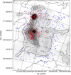 |
Fig. 5 IRAS maps of Chamaeleon I region in 100 μm flux (Schlegel et al. 1998). The six contours range from 8 to 30 MJy/sr. Red stars represent the known members of ChamaeleonI taken from Luhman (2007) and Luhman & Muench (2008). Blue circles indicate the TGAS stars selected for our analysis. |
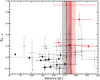 |
Fig. 6 Extinction distribution along the line of sight for stars located on the line of sight of the Chamaeleon I cloud. The dashed line represents the position of the front edge of the cloud determined by the reddening turn-on method and the gray shaded region its 1σ uncertainty. The red dotted line indicates the average distance of the members, shown here for comparison, and the red shaded region indicates the 1σ uncertainty on this value, either statistical (darker red region) or systematic (lighter red region). The members of the Chamaeleon I region are represented with stars, the field stars for which both the spectral type and luminosity class are reported in the literature are shown with circles, whereas triangles indicate objects for which we estimate the luminosity class ourselves. Symbols colored in red indicate the stars with color excess larger than 0 at 3σ, in black withcolor excess <0.2, and those in gray indicate the uncertainties too large to be considered in either of these two categories. We highlight with black circles the stars used to compute the distance of the reddening turn-on, thus the front edge of the cloud. |
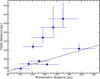 |
Fig. 7 Comparison of photometric distances (dphot) vs. TGAS distances (dTGAS) for the Whittet et al. (1997) stars that are relevant for the computation of the onset. The black line represents dTGAS = dphot. |
3.2 Chamaeleon II
The distance of the Chamaeleon II cloud is derived here using solely the reddening turn-on method, since no members of this region are included in the TGAS catalog owing to their faintness. Figure 8 shows the position of the known members of the Chamaeleon II region and of the 44 stars included in the TGAS catalog located on the line of sight of this region and used forthe analysis.
Both the spectral type and luminosity class are available from the literature for 28 of the TGAS stars on the line of sight of the Chamaeleon II cloud. For the remaining stars, the luminosity class is missing in five cases and only the effective temperature is reported for 11 stars. These luminosity classes are computed as discussed in Appendix A, and we find thatthey are always dwarfs, apart from two cases where they are between subgiants and dwarfs (see Table 4).
We thus computed the E(B − V ) color excess for these targets, and this is shown as a function of their distance in Fig. 9. The distance of the reddening turn-on, and thus of the front-edge of the cloud, is found to be at a parallax of 5.53 ± 0.16 mas, corresponding to a distance of
![Mathematical equation: \begin{equation*} d_{\textrm{Chamaeleon\ II}} = 181^{+6+11}_{-5-10} \ \textrm{[pc]}, \nonumber \end{equation*}](/articles/aa/full_html/2018/02/aa31153-17/aa31153-17-eq23.png)
which is well compatible with the previous estimate of 178 ± 18 pc by Whittet et al. (1997), and definitely rules out the hypothesis of much larger distances of 400 pc previously claimed for this cloud.
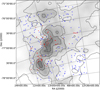 |
Fig. 8 IRAS 100 μm flux maps of Chamaeleon II region. The six contours range from 8 to 30 MJy/sr. Red stars represent the confirmed members of Chamaeleon II reported in Spezzi et al. (2008). Blue circles indicate the TGAS stars in this field of view. |
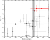 |
Fig. 9 Color excess as a function of distance for stars included in the TGAS catalog and located on the line of sight of the Chamaeleon II cloud. The dashed line represents the position of the cloud front edge, and the gray shaded region its uncertainty. Other symbols are as in Fig. 6. |
3.3 Chamaeleon III
The Chamaeleon III region is less studied than the previous regions and no information about its young stellar population is available. We thus selected, for distance analyses, the 39 stars included in the TGAS catalog that are located on the line of sight of the cloud, as shown in Fig. 10. We were only able to find both the spectral type and luminosity class information in the literature for nine of these stars, while we determined the luminosity class for nine additional stars missing this information, and for the remaining 21 stars for which only the effective temperature is reported. As discussed in Appendix A, all but five of these stars are main-sequence stars, while the others are in between subgiants and dwarfs in three cases, and subgiants in the last two cases (see Table 5).
We computed the color excess for all these stars and showed it versus their distances in Fig. 11. This allowed us to locate the distance of the front edge of the cloud at a parallax of 5.19 ± 0.21 mas, corresponding to a distance of
![Mathematical equation: \begin{equation*} d_{\textrm{Chamaeleon\ III}} = 193 ^{+8+12}_{-7-11} \ \textrm{[pc]}. \nonumber \end{equation*}](/articles/aa/full_html/2018/02/aa31153-17/aa31153-17-eq24.png)
Compared to the distances to the other clouds, this value is to be considered slightly more uncertain owing to the higher level of structuring of this cloud (see Fig. 10). It is possible that some denser cloudlets are closer, which makes the analysis more uncertain4. Furthermore, a smaller number of stars are available for the analysis. In any case, this value represents the first ever estimate of the distance of this cloud and confirms that its distance is compatible with the distances of the other two clouds, although the nominal value is ~10–15 pc further away. This result suggests that it is possible that these three Chamaeleon clouds are higher density star-forming regions of a single larger cloud structure.
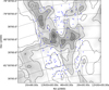 |
Fig. 10 IRAS maps of Chamaeleon III region in 100 μm flux. The six contours range from 8 to 30 MJy/sr. Blue circles indicate the TGAS stars in this field of view. |
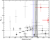 |
Fig. 11 Color excess vs. distance for the stars located on the line of sight of the Chamaeleon III cloud. The black dashed line represents the position of the cloud front edge, while the blue dashed line indicates the distance to the Chamaelon I and II clouds. Other symbols are as in Fig. 6. |
3.4 Musca
The Musca cloud is an elongated and much narrower structure in the sky than the Chamaeleon clouds. We show the extent of this cloud in Fig. 12, together with the position of the 76 stars included in the TGAS catalog,which are selected to determine the reddening turn-on distance for this cloud. For only six of these stars, both the spectral type and luminosity class are reported in the literature, while for the remaining 70 stars only the effective temperatureis available, and we derive their luminosity class as discussed in Appendix A. We find that 20 of these stars are dwarfs, one is in between subgiant and dwarf, 22 are subgiants, and 27 are giants (see Table 6).
The analysis of the color excess versus distance for these 76 stars, shown in Fig. 13, does not allow us to constrain the distance of the front edge of the Musca cloud. We can only infer the mean parallax of the two closest significantly reddened stars, which is found to be 1.66 ± 0.22, corresponding to a distance of  pc. This can be considered as an upper limit on the distance to this cloud. The impossibility of deriving a more stringent constraint on the distance to this cloud is due to the large uncertainties on the color excess of the stars on the line of sight; this is mainly because only the effective temperature is available for the vast majority of these stars and because these temperatures are in many cases photometrically computed, thus more uncertain.
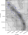 |
Fig. 12 IRAS maps of Musca region in 100 μm flux. The six contours range from 8 to 30 MJy/sr. Blue circles indicate the TGAS stars in this field of view. |
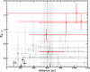 |
Fig. 13 Extinction distribution along the line of sight of Musca. Symbols as in Fig. 6. The dashed line indicates the inverted mean value of the parallaxes of the first two reddened stars, with its statistical uncertainty shown with a gray region. |
3.5 Summary
We report the final distances to three of the four clouds that we analyzed in Table 7. The distances to the Chamaeleon I is found to be ~20 pc larger than previously assumed, although the difference is still compatible within the measurement uncertainties. On the contrary, the Chamaeleon II cloud is confirmed to be at a distance of ~180 pc, and is foundto be almost at the same distance as the Chamaeleon I cloud.
We are able to report for the first time a distance estimate to the Chamaeleon III cloud, which is consistent with the idea that the three Chamaeleon clouds are part of a single cloud structure and significantly larger than the previously assumed distance to this cloud. Finally, the distance to the Musca cloud is only loosely constrained to be closer than 600 pc with a large uncertainty.
Summary of the distances to the clouds studied here.
4 Discussion
4.1 Impact of the new distance estimate on stellar properties of Chamaeleon I stars
As noted in the introduction, the distance is a key parameter in the computation of several stellar properties, in particular the stellar luminosity (L⋆). This value is used together with the effective temperature and evolutionary models to derive the stellar mass (M⋆) and age. We determined that the distance to the Chamaeleon I region is  pc, and not 160 ± 15 pc as previously assumed. Although the two values are compatible within their uncertainties, we explored the impact of the difference in the nominal value of the distance on the stellar properties of the young stellar objects in this region.
In the following, we use the values of L⋆ determined with spectroscopy and assuming a distance of 160 pc by Manara et al. (2016, 2017). The stellar luminosity is modified by a factor equal to the squared ratio of the new and previous distance estimate 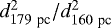 . This implies that L⋆ is higher by 25% owing to the larger distance estimate. The difference in the values of L⋆ is shown on the Hertzsprung-Russel diagram (HRD) in Fig. 14. The values of L⋆ obtained with the newly derived distance to the Chamaeleon I region are still compatible within 1σ with those using the previously used distance.
In turn,the mass and age of the stars are also affected by the different value of the distance to the region, and we compute the new values using the evolutionary models by Baraffe et al. (2015). The variations on the stellar masses are negligible, since this value mainly depends on the temperature of the stars for low mass stars at this evolutionary stage (cf. Fig. 14), which is unaffected by the distance estimate. On the contrary, the age estimate using the new distance suggests that the Chamaeleon I stellar population is ≲1 Myr younger than previously found.
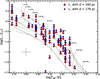 |
Fig. 14 Hertzsprung Russel diagram (HRD) of young stars with disks in the Chamaeleon I region studied by Manara et al. (2016, 2017). The red diamonds and blue circles indicate L⋆ computed with the distance of 160 pc found by Whittet et al. (1997) with our distance of 179 pc, respectively. Typical uncertainties are shown with a cross in the bottom left corner. The evolutionary models (isochrones in solid lines and evolutionarytracks with dashed lines) are taken from Baraffe et al. (2015). |
4.2 Connection between the Chameleon clouds and large-scale structures
Now that the distance of the three Chamaeleon clouds is constrained we put this information together with the position of these clouds in Galactic coordinates to investigate the connection between these clouds and large-scale structures in the Milky Way galaxy.
We have shown that the Chamaeleon I and Chamaeleon II clouds are both at ~180 pc from us, while the Chamaeleon III region is slightly further away. According to Corradi et al. (1997), there is negligible interstellar material between us and the Chamaeleon-Musca complex, as observed by the low extinction measured. Thus, emission from dust particles should arise from clouds located at the same distance or further away than the Chamaeleon-Musca complex. We show in Fig. 15 a dust density map of this complex, which shows the presence of dust structures connecting the three Chamaeleon clouds with each other and the Musca cloud. This structure could represent a physical link between the clouds.
We discuss the connection between this structure and larger scale structures in the context of two hypotheses reported in the literature. King et al. (1979) observed the nebulosity structures in the vicinity of the southern celestial pole and proposed the existence of a sheet-like structure of clouds extending in parallel to the Galactic plane and southward from it with a distance of between 40 and 80 pc from the plane. On the contrary, Corradi et al. (1997) investigated the color excess as a function of distance in a large region of the sky ranging from the Southern Coalsack (l =300°, b = 0°) to the Chamaeleon-Musca complex (l = 300°, b = −15°). They found evidence of a possible physical association between these two structures, and thus hypothesized the existence of a sheet-like structure of clouds perpendicular to the Galactic plane. They suggested that these clouds could be overdensities formed at the interface between the Local and Loop I bubbles.
We represent our results and these two hypotheses with a scheme in Fig. 16. The distance to the sheet of clouds parallel to the Galactic plane (zs ) and the distance to the sheet of clouds perpendicular to it (xs) are obtained using the following equations:
 (6)
(6)
where d is the distance and b the Galacticlatitude of the clouds.
We can determine the distance from the Galactic plane to the sheet of clouds parallel to it (King et al. 1979), and the distance from the Sun to the sheet of clouds perpendicular to the Galactic plane (Corradi et al. 1997) using the distance to the three Chamaeleondark clouds. The values obtained with the distance to each of the clouds are reported in Table 8. All three estimates of the distance of the hypothetical parallel sheet of clouds from the Galactic plane are consistent with each other within 2σ at most, which is similar to the distances of the perpendicular sheet of clouds from the Sun. Thus, we cannot distinguish between the two hypotheses solely based on the measured distances to the three Chamaeleon clouds.
Independent information on the distance to the Southern Coalsack region leads us to consider the hypothesis that a sheet of clouds perpendicular to the Galactic plane is a viable possibility. This region is located at Galactic latitude b = 0°, and thus xs corresponds to its distance (see Eq. (6)). The distance to this region was measured by Rodgers (1960) and Franco (1989) to be 174 ± 18 pc and 180 ± 26 pc, respectively. These values are well compatible with the values of xs derived hereusing the distance to the Chamaleon I and II clouds, which supports the hypothesis of the existence of a sheet of clouds perpendicular to the Galactic plane. However, we cannot with our data discard either of the two hypotheses or the possibility that both structures exist.
Finally, we try to put more stringent constraints on the distance to the Musca cloud in the context of the two hypotheses of large-scale structures we discussed. By knowing the Galactic latitude of this region (b = −9°) and assuming the values ofxs and zs of Table 8, we can invert Eq. (6) to infer a distance to the Musca cloud. The result of this exercise is a distance dparallel = 311 ± 54 pc or dperpendicular = 179 ± 7 pc according tothe two hypotheses, respectively. Both values are well consistent with the loose upper limit we have derived from the color excess analysis.
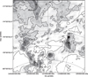 |
Fig. 15 IRAS 100 μm flux map of Chamaeleon-Musca region. The six contours range from 8 to 30 MJy/sr. |
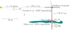 |
Fig. 16 Schematic view of the large-scale structure of the dust clouds in the direction of the Chamaeleon-Musca complex. The location of the Sun is represented with a yellow circle, while the blue, red, green, and black points represent the location of the three Chamaeleon clouds and Southern Coalsack dark cloud, respectively, derived using the distances from our work in the case of the Chamaeleon clouds, and the Galactic coordinates of the objects. The large gray and green cloud are the dust and gas hypothetical structure proposed by King et al. (1979) and Corradi et al. (1997), respectively, as discussed in the text. |
Values zs and xs for the studied clouds.
5 Conclusions
In this work we used the newly released data from the Data Release 1 of the Gaia satellite, in particular the parallax estimates from the TGAS catalog, to constrain the distance to the four main clouds in the Chamaeleon-Musca complex. Owing to the limiting magnitude of the TGAS catalog we were able to derive a distance by directly computing the mean value of the distances to members only in the Chamaeleon I cloud. This analysis of the distances to the members led us to estimate a distance of  pc for this cloud, where the errors are statistical and systematic, respectively.
We then combined the parallax values from the TGAS catalog for stars on the line of sight of the Chamaeleon-Musca clouds with measurements of their E(B − V ) color excess. By measuring the parallax at which we observe an increase of the color excess to values larger than zero we were able to locate the front edge of the cloud and thus to infer its distance. This method allows us to measure a distance of  pc to the Chamaeleon I cloud, which is compatible with the distance to the members and further away than the previously assumed distance to this cloud. A discrepency in the photometric distance estimates with respect to the TGAS distances causes this difference; this shows the importance of parallax based distances for the analysis. Furthermore, we confirm the distance to the Chamaeleon II cloud with the reddening turn-on method and measure a distance of
  pc, consistent with that to the Chamaeleon I cloud. We are then able to measure for the first time the distance to the Chamaeleon III cloud, which is found to be
  pc and only to suggest that the distance to the Musca cloud is smaller than
  pc.
pc.
The newly estimated further distance to the Chamaeleon I cloud results in an increase of the stellar luminosities of 25%, which implies a slightly younger age for this region by ≲1 Myr, but it affects the other stellar properties only within their uncertainties.
Finally, we discussed the relation of the clouds in the Chamaeleon-Musca region with two different possible large-scale cloud structures hypothesized in the literature, namely, a sheet of cloud parallel or perpendicular to the Galactic plane. The distances we measured to the three Chamaeleon clouds, combined with their Galactic coordinates, do not allow us to rule out either of the hypotheses. In the context of these hypotheses, we compute two possible distances to the Musca cloud, namely, dparallel = 311 ± 54 pc and dperpendicular = 179 ± 7 pc.
The major limitation of our study is represented by the limited number of members of the targeted clouds included in the TGAS catalog, mainly because of the limiting magnitude of this catalog. This limitation will be largely overcome by the future Gaia Data Release 2, which is planned for April 2018. Parallaxes for stars as faint as G ~ 20 mag will be included and will allow us to use the distance to a larger number of members to derive the distances to nearby star -forming regions (d ≲ 300 pc). On the other hand, we will be able to apply the reddening turn-on method to star-forming clouds even in the cases where the members of the region are too faint to be included in the Gaia catalog, for example, where most of their members are still embedded in their envelope or where star formation has not started yet.
Acknowledgements
This work has made use of data from the European Space Agency (ESA) mission Gaia (http://www.cosmos.esa.int/gaia), processed by the Gaia Data Processing and Analysis Consortium (DPAC, http://www.cosmos.esa.int/web/gaia/dpac/consortium). Funding for the DPAC has been provided by national institutions, in particular the institutions participating in the Gaia Multilateral Agreement. This research has made use of the SIMBAD database, operated at CDS, Strasbourg, France. J.V. acknowledges the ESA trainee program and C.F.M. acknowledges an ESA research fellowship funding. We acknowledge a detailed and constructive anonymous referee report, which significantly improved the paper. Finally, we would like to thank Jos De Bruijne, Eleonora Zari, and Stella Reino for their stimulating comments.
Appendix A: Color magnitude diagrams to determine luminosity classes of stars
Our methodof deriving distances to dark clouds from the determination of the reddening turn-on distance relies on the availabilityof spectral type, luminosity class, photometry, and distance for each star on the line of sight. We describe how we derived the luminosity class for the targets when this is not available in the literature. We converted the observed V magnitude of the targets into absolute magnitude using the parallax estimates from the TGAS catalog converted into distances as discussed byAstraatmadja & Bailer-Jones (2016). We used the standard deviation on the mode of the posteriors as an uncertainty on the distance. This value is well in line with using the 5 and 95 percentile of the posteriors for small parallax errors, as in the majority of the stars used here. Small differences in these uncertainties causing a misclassification do not affect the results significantly, as we discuss in the following. We used this information together with the B − V color to locate the stars on the color-magnitude diagram (CMD). Then, we compared the location of the stars on the CMD with the color and magnitudes reported for different luminosity classes by Pecaut & Mamajek (2013) for dwarfs (V) and K1-M5 subgiants (IV) and by Gottlieb (1978) for earlier type subgiants, giants (III), and luminosity classes I and II.
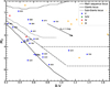 |
Fig. A.1 Absolute V magnitude vs. B − V color for the stars on the line of sight of the Chamaeleon I cloud with known spectral type and luminosity class, as labeled. The black line represents the main-sequence locus, the dashed line represents the Giants locus, and the dotted line the subgiants locus (Pecaut & Mamajek 2013; Gottlieb 1978, see text for details). The dashed and dotted lines represent the limit between luminosity classes V, IV/V, and IV. The black arrow indicates the reddening vector. |
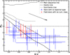 |
Fig. A.2 Absolute V magnitude vs. B − V color for the stars on the line of sight of the Chamaeleon I cloud without an estimate of the luminosity class. Red symbols indicate stars with spectral types derived from spectroscopy and missing the luminosity class, while blue symbols indicate only when the effective temperature is available. Lines are as in Fig. A.1. |
Figure A.1 shows the CMD for stars on the line of sight of the Chamaeleon I cloud, for which both the spectral type and luminosity class are reported in the literature. This diagram confirms that the luminosity class estimated in the literature agrees with the loci expected for the different luminosity classes with only a few outliers. However, a misclassification in the luminosity class between subgiants and dwarfs would have a limited effect on the color excess value. Indeed, the difference in E(B − V ) between a B8V star and a B8IV star is 0.018 mag and is similar for other spectral types. This uncertainty is included in the error budget and does not affect substantially our analysis. Finally, the reddening vector is parallel to the dwarf and subgiant locus, as shown on Fig. A.1, thus increasing values of extinction do not affect our results.
The CMDs used to determine the luminosity class for stars on the line of sight of the four clouds analyzed here are shown in Figs. A.2–A.5 for the Chamaeleon I, II, III, and Musca clouds, respectively. Most of the stars in the line of sight of the Chamaeleon I and II have luminosity class V with only two exceptions in each region. In the Chamaleon III line of sight,instead, seven stars are not of luminosity class V, and an higher fraction of luminosity classes III and IV are present on the line of sight of the Musca cloud.
Appendix B: Discrepancies between photometric distances and TGAS distances
The previous estimate of the distance to the Chamaeleon I cloud of 160 ± 15 pc was obtained by Whittet et al. (1997) using the same reddening turn-on method as used by us. We investigate the origin of the different estimates, which is related to the difference in the distances estimated from the TGAS parallax versus the photometric distances used by Whittet et al. (1997), shown in Fig. B.1 for the stars in common in the two works. These values are reported in Table B.1. While there is an agreement between the two methods for four stars with distances smaller than 150 pc and for one star at ~200 pc, there are four additional stars (TYC 9414-642-1, TYC 9410-2627-1, TYC 9410-2608-1, TYC 9411-998-1) for which the two methods do not agree, where the TGAS distances are significantly larger. These stars were considered to be in front of the cloud by Whittet et al. (1997) based on the photometric distances, while they appear to be behind the cloud with the TGAS estimates.
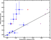 |
Fig. B.1 Distances estimated from TGAS parallax measurements vs. photometric distances used by Whittet et al. (1997) for the same stars, shown with blue points. Red diamonds show the photometric distance computed assuming RV = 3.1, and purple triangles indicate the same value correcting the luminosity class of the targets using their position on the CMD in Fig. B.2. |
Objects used in the comparison.
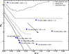 |
Fig. B.2 Color magnitude diagram of the stars in Table B.1. The absolute magnitude are computed using the TGAS distances and the B and V are taken from Høg et al. (2000). The Tycho 2 id and spectral classification (Whittet et al. 1997) of each star are reported and the luminosity class corresponding to the position on the CMD is computed with the TGAS distance. |
We first explore the possibility that the differences are due to the reddening law assumed by Whittet et al. (1997) and used to compute the photometric distance. They assumed a value of RV = 1.1 × E(V − K)∕E(B − V ), which results in very different values from one target to another. We thus assume RV = 3.1 for all the stars and recalculate their photometric distances. As shown in Fig. B.1, the differences in the photometric distances are too small to explain the discrepancy between the two methods.
We thus consider the hypothesis that the luminosity class of the stars was incorrectly estimated, and for this aim we show in Fig. B.2 the CMD of the stars in Table B.1, where the absolute V magnitudes are computed using the TGAS distances. The four F-type dwarfs and the K-type giant are the five stars for which the distances derived with the two methods are compatible. Also their positions on the CMD is always consistent with the luminosity class assumed by Whittet et al. (1997). Similarly, the G-type subgiant is still consistent with the previously assumed luminosity class, and thus the discrepancy between the photometric distance and the TGAS distance cannot be explained with this argument. On the contrary, we find that the luminosity class was incorrectly estimated for the remaining three stars with discrepancy in the distances estimates with the two methods. Once we compute the photometric distances with the correct luminosity class and assuming RV = 3.1 (Fig. B.1) we find a better agreement between this distance and the TGAS distances.
We conclude that the reason for the different estimate of the distance to the Chamaeleon I cloud is due to the incorrect estimateof the photometric distance of four stars in the work by Whittet et al. (1997), which led the authors to derive a closer distance to this region. The reason for the erroneously estimated photometric distances is due to a wrong luminosity class determination for these targets. Once error is corrected, the agreement between the TGAS and photometric distances is good. This shows the importance of having distances estimates derived from parallaxes, as these are independent of the stellar parameters.
References
- Alonso, A., Arribas, S., & Martínez-Roger, C. 1999, A&AS, 140, 261 [NASA ADS] [CrossRef] [EDP Sciences] [Google Scholar]
- Ammons, S. M., Robinson, S. E., Strader, J., et al. 2006, ApJ, 638, 1004 [NASA ADS] [CrossRef] [Google Scholar]
- Andersson, B.-G., Pintado, O., Potter, S. B., Straižys, V., & Charcos-Llorens, M. 2011, A&A, 534, A19 [NASA ADS] [CrossRef] [EDP Sciences] [Google Scholar]
- Appenzeller, I. 1977, A&A, 61, 21 [NASA ADS] [Google Scholar]
- Astraatmadja, T. L., & Bailer-Jones, C. A. L. 2016, ApJ, 833, 119 [NASA ADS] [CrossRef] [Google Scholar]
- Bailer-Jones, C. A. L. 2015, PASP, 127, 994 [NASA ADS] [CrossRef] [Google Scholar]
- Baraffe, I., Homeier, D., Allard, F., & Chabrier, G. 2015, A&A, 577, A42 [NASA ADS] [CrossRef] [EDP Sciences] [Google Scholar]
- Bastian, U., & Röser, S. 1993, PPM Star Catalogue. Positions and proper motions of 197179 stars south of –2.5 degrees declination for equinox and epoch J2000.0. Vol. III: Zones -00 to –20 degrees, Vol. IV: Zones –30 to –80 degrees [Google Scholar]
- Bijaoui, A., Recio-Blanco, A., De Laverny, P., & Ordenovic, C. 2012, Statistical Methodology, 9, 55 [Google Scholar]
- Corradi, W. J. B., Franco, G. A. P., & Knude, J. 1997, A&A, 326, 1215 [NASA ADS] [Google Scholar]
- Cox, N. L. J., Arzoumanian, D., André, P., et al. 2016, A&A, 590, A110 [NASA ADS] [CrossRef] [EDP Sciences] [Google Scholar]
- de Zeeuw, P. T., Hoogerwerf, R., de Bruijne, J. H. J., Brown, A. G. A., & Blaauw, A. 1999, AJ, 117, 354 [NASA ADS] [CrossRef] [Google Scholar]
- Franco, G. A. P. 1989, A&A, 215, 119 [NASA ADS] [Google Scholar]
- Franco, G. A. P. 1991, A&A, 251, 581 [NASA ADS] [Google Scholar]
- Gaia Collaboration (Brown, A. G. A., et al.) 2016a, A&A 595, A2 [NASA ADS] [CrossRef] [EDP Sciences] [Google Scholar]
- Gaia Collaboration (Prusti, T., et al.) 2016b, A&A 595, A1 [NASA ADS] [CrossRef] [EDP Sciences] [Google Scholar]
- Gottlieb, D. M. 1978, ApJS, 38, 287 [NASA ADS] [CrossRef] [Google Scholar]
- Graham, J. A., & Hartigan, P. 1988, AJ, 95, 1197 [NASA ADS] [CrossRef] [Google Scholar]
- Gustafsson, B., Edvardsson, B., Eriksson, K., et al. 2008, A&A, 486, 951 [NASA ADS] [CrossRef] [EDP Sciences] [Google Scholar]
- Høg, E., Fabricius, C., Makarov, V. V., et al. 2000, A&A, 355, L27 [Google Scholar]
- Houk, N., & Cowley, A. P. 1975, University of Michigan Catalogue of two-dimensional spectral types for the HD stars. Volume I [Google Scholar]
- Hughes, J., & Hartigan, P. 1992, AJ, 104, 680 [NASA ADS] [CrossRef] [Google Scholar]
- Irvine, N. J., & Houk, N. 1977, PASP, 89, 347 [NASA ADS] [CrossRef] [Google Scholar]
- Jackson, J., & Stoy, R. H. 1996, VizieR Online Data Catalog: I/116 [Google Scholar]
- King, D. J., Taylor, K. N. R., & Tritton, K. P. 1979, MNRAS, 188, 719 [NASA ADS] [Google Scholar]
- Kordopatis, G., Gilmore, G., Steinmetz, M., et al. 2013, AJ, 146, 134 [NASA ADS] [CrossRef] [Google Scholar]
- Lopez Martí, B., Jimenez Esteban, F., Bayo, A., et al. 2013, A&A, 551, A46 [NASA ADS] [CrossRef] [EDP Sciences] [Google Scholar]
- Luhman, K. L. 2004, ApJ, 602, 816 [NASA ADS] [CrossRef] [Google Scholar]
- Luhman, K. L. 2007, ApJS, 173, 104 [Google Scholar]
- Luhman, K. L. 2008, Chamaeleon, ed. B. Reipurth, 2, 169 [Google Scholar]
- Luhman, K. L., & Muench, A. A. 2008, ApJ, 684, 654 [NASA ADS] [CrossRef] [Google Scholar]
- Manara, C. F., Fedele, D., Herczeg, G. J., & Teixeira, P. S. 2016, A&A, 585, A136 [NASA ADS] [CrossRef] [EDP Sciences] [Google Scholar]
- Manara, C. F., Testi, L., Herczeg, G. J., et al. 2017, A&A, 604, A127 [NASA ADS] [CrossRef] [EDP Sciences] [Google Scholar]
- Nesterov, V. V., Kuzmin, A. V., Ashimbaeva, N. T., et al. 1995, A&AS, 110, 367 [NASA ADS] [Google Scholar]
- Pecaut, M. J., & Mamajek, E. E. 2013, ApJS, 208, 9 [NASA ADS] [CrossRef] [Google Scholar]
- Perrin, G., Coudé du Foresto, V., Ridgway, S. T., et al. 1998, A&A, 331, 619 [NASA ADS] [Google Scholar]
- Perryman, M. A. C., Lindegren, L., Kovalevsky, J., et al. 1997, A&A, 323, L49 [NASA ADS] [Google Scholar]
- Recio-Blanco, A., Bijaoui, A., & de Laverny P. 2006, MNRAS, 370, 141 [NASA ADS] [CrossRef] [Google Scholar]
- Rodgers, A. W. 1960, MNRAS, 120, 163 [NASA ADS] [CrossRef] [Google Scholar]
- Schlegel, D. J., Finkbeiner, D. P., & Davis, M. 1998, ApJ, 500, 525 [NASA ADS] [CrossRef] [Google Scholar]
- Schwartz, R. D. 1992, The Chamaeleon Dark Clouds and T-Associations, ed. B. Reipurth, 93 [Google Scholar]
- Spezzi, L., Alcalá, J. M., Covino, E., et al. 2008, ApJ, 680, 1295 [NASA ADS] [CrossRef] [Google Scholar]
- Torres, C. A. O., Quast, G. R., da Silva, L., et al. 2006, A&A, 460, 695 [NASA ADS] [CrossRef] [EDP Sciences] [Google Scholar]
- van Leeuwen F. 2007, A&A, 474, 653 [NASA ADS] [CrossRef] [EDP Sciences] [Google Scholar]
- Vrba, F. J., & Rydgren, A. E. 1984, ApJ, 283, 123 [NASA ADS] [CrossRef] [Google Scholar]
- Wenger, M., Ochsenbein, F., Egret, D., et al. 2000, A&AS, 143, 9 [NASA ADS] [CrossRef] [EDP Sciences] [Google Scholar]
- Whittet, D. C. B., Kirrane, T. M., Kilkenny, D., et al. 1987, MNRAS, 224, 497 [NASA ADS] [CrossRef] [Google Scholar]
- Whittet, D. C. B., Prusti, T., Franco, G. A. P., et al. 1997, A&A, 327, 1194 [NASA ADS] [Google Scholar]
The maps are taken from the NASA/IPAC Infrared Science Archive (IRSA) website http://irsa.ipac.caltech.edu/applications/DUST/
The effective temperatures for the stars with no spectral type are either from Kordopatis et al. (2013) or Ammons et al. (2006). In Kordopatis et al. (2013) the effective temperatures were deduced from spectroscopy using a combination of two different algorithms, a projection method called MATISSE (Recio-Blanco et al. 2006) and a decision-tree method called DEGAS (Bijaoui et al. 2012). The spectra of the stars are fitted to synthesized MARCS model atmospheres (Gustafsson et al. 2008). In Ammons et al. (2006) the effective temperatures were photometrically computed using a χ2 -optimized fitting polynomials method. Perrin et al. (1998) and Alonso et al. (1999) also used photometric determination by utilizing a minimization method.
All TGAS parallaxes have a systematic uncertainty of 0.3 mas (Gaia Collaboration 2016a). This is already included in the individual uncertainties on parallaxes in the TGAS catalog, but it affects any mean value as well, and is therefore always reported in this work.
The well-known T Cha star is projected between Chamaeleon III and Chamaleon I in the sky, but this star is actually in the foreground at d = 107 pc.
All Tables
HIPPARCOS and TGAS parallaxes and inferred distances of the five members of Chamaeleon I included in both catalogs.
All Figures
|
Fig. 1 Gaia star density map of the Chamaeleon-Musca region. The figure is a 11° × 13° field centered on the coordinates (l = 300.5°, b = −13.3°). |
| In the text | |
|
Fig. 2 Comparison of |
| In the text | |
|
Fig. 3 Top: TGAS parallaxes (πTGAS) vs. HIPPARCOS parallaxes (πHip) to the five members of Chamaeleon I included in both HIPPARCOS catalog (van Leeuwen 2007) and TGAS catalog (Gaia Collaboration 2016a). The black line represents the one to one relation. Bottom: same for distances, taken as inverse of the parallax for HIPPARCOS data and from Astraatmadja & Bailer-Jones (2016) for TGAS (see Table 1). Uncertainties on both axes are as discussed in Table 1, and they correspond to 1σ uncertainty for the HIPPARCOS values and 2σ for TGAS. |
| In the text | |
|
Fig. 4 IRAS maps of the Chamaeleon I region at 100 μm (Schlegel et al. 1998). The six contours range from 8 MJy/sr to 30 MJy/sr. The positions of the members of this region included in the TGAS catalog are represented with red circles. The red arrows represent their displacement in 105 yr. The Tycho-2 or HIPPARCOS name and TGAS distance of each star are reported as labels for each object. |
| In the text | |
|
Fig. 5 IRAS maps of Chamaeleon I region in 100 μm flux (Schlegel et al. 1998). The six contours range from 8 to 30 MJy/sr. Red stars represent the known members of ChamaeleonI taken from Luhman (2007) and Luhman & Muench (2008). Blue circles indicate the TGAS stars selected for our analysis. |
| In the text | |
|
Fig. 6 Extinction distribution along the line of sight for stars located on the line of sight of the Chamaeleon I cloud. The dashed line represents the position of the front edge of the cloud determined by the reddening turn-on method and the gray shaded region its 1σ uncertainty. The red dotted line indicates the average distance of the members, shown here for comparison, and the red shaded region indicates the 1σ uncertainty on this value, either statistical (darker red region) or systematic (lighter red region). The members of the Chamaeleon I region are represented with stars, the field stars for which both the spectral type and luminosity class are reported in the literature are shown with circles, whereas triangles indicate objects for which we estimate the luminosity class ourselves. Symbols colored in red indicate the stars with color excess larger than 0 at 3σ, in black withcolor excess <0.2, and those in gray indicate the uncertainties too large to be considered in either of these two categories. We highlight with black circles the stars used to compute the distance of the reddening turn-on, thus the front edge of the cloud. |
| In the text | |
|
Fig. 7 Comparison of photometric distances (dphot) vs. TGAS distances (dTGAS) for the Whittet et al. (1997) stars that are relevant for the computation of the onset. The black line represents dTGAS = dphot. |
| In the text | |
|
Fig. 8 IRAS 100 μm flux maps of Chamaeleon II region. The six contours range from 8 to 30 MJy/sr. Red stars represent the confirmed members of Chamaeleon II reported in Spezzi et al. (2008). Blue circles indicate the TGAS stars in this field of view. |
| In the text | |
|
Fig. 9 Color excess as a function of distance for stars included in the TGAS catalog and located on the line of sight of the Chamaeleon II cloud. The dashed line represents the position of the cloud front edge, and the gray shaded region its uncertainty. Other symbols are as in Fig. 6. |
| In the text | |
|
Fig. 10 IRAS maps of Chamaeleon III region in 100 μm flux. The six contours range from 8 to 30 MJy/sr. Blue circles indicate the TGAS stars in this field of view. |
| In the text | |
|
Fig. 11 Color excess vs. distance for the stars located on the line of sight of the Chamaeleon III cloud. The black dashed line represents the position of the cloud front edge, while the blue dashed line indicates the distance to the Chamaelon I and II clouds. Other symbols are as in Fig. 6. |
| In the text | |
|
Fig. 12 IRAS maps of Musca region in 100 μm flux. The six contours range from 8 to 30 MJy/sr. Blue circles indicate the TGAS stars in this field of view. |
| In the text | |
|
Fig. 13 Extinction distribution along the line of sight of Musca. Symbols as in Fig. 6. The dashed line indicates the inverted mean value of the parallaxes of the first two reddened stars, with its statistical uncertainty shown with a gray region. |
| In the text | |
|
Fig. 14 Hertzsprung Russel diagram (HRD) of young stars with disks in the Chamaeleon I region studied by Manara et al. (2016, 2017). The red diamonds and blue circles indicate L⋆ computed with the distance of 160 pc found by Whittet et al. (1997) with our distance of 179 pc, respectively. Typical uncertainties are shown with a cross in the bottom left corner. The evolutionary models (isochrones in solid lines and evolutionarytracks with dashed lines) are taken from Baraffe et al. (2015). |
| In the text | |
|
Fig. 15 IRAS 100 μm flux map of Chamaeleon-Musca region. The six contours range from 8 to 30 MJy/sr. |
| In the text | |
|
Fig. 16 Schematic view of the large-scale structure of the dust clouds in the direction of the Chamaeleon-Musca complex. The location of the Sun is represented with a yellow circle, while the blue, red, green, and black points represent the location of the three Chamaeleon clouds and Southern Coalsack dark cloud, respectively, derived using the distances from our work in the case of the Chamaeleon clouds, and the Galactic coordinates of the objects. The large gray and green cloud are the dust and gas hypothetical structure proposed by King et al. (1979) and Corradi et al. (1997), respectively, as discussed in the text. |
| In the text | |
|
Fig. A.1 Absolute V magnitude vs. B − V color for the stars on the line of sight of the Chamaeleon I cloud with known spectral type and luminosity class, as labeled. The black line represents the main-sequence locus, the dashed line represents the Giants locus, and the dotted line the subgiants locus (Pecaut & Mamajek 2013; Gottlieb 1978, see text for details). The dashed and dotted lines represent the limit between luminosity classes V, IV/V, and IV. The black arrow indicates the reddening vector. |
| In the text | |
|
Fig. A.2 Absolute V magnitude vs. B − V color for the stars on the line of sight of the Chamaeleon I cloud without an estimate of the luminosity class. Red symbols indicate stars with spectral types derived from spectroscopy and missing the luminosity class, while blue symbols indicate only when the effective temperature is available. Lines are as in Fig. A.1. |
| In the text | |
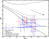 |
Fig. A.3 Same as Fig. A.2 for stars on the line of sight of the Chamaeleon II cloud. |
| In the text | |
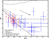 |
Fig. A.4 Same as Fig. A.2 for stars on the line of sight of the Chamaeleon III cloud. |
| In the text | |
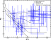 |
Fig. A.5 Same as Fig. A.2 for stars on the line of sight of the Musca cloud. |
| In the text | |
|
Fig. B.1 Distances estimated from TGAS parallax measurements vs. photometric distances used by Whittet et al. (1997) for the same stars, shown with blue points. Red diamonds show the photometric distance computed assuming RV = 3.1, and purple triangles indicate the same value correcting the luminosity class of the targets using their position on the CMD in Fig. B.2. |
| In the text | |
|
Fig. B.2 Color magnitude diagram of the stars in Table B.1. The absolute magnitude are computed using the TGAS distances and the B and V are taken from Høg et al. (2000). The Tycho 2 id and spectral classification (Whittet et al. 1997) of each star are reported and the luminosity class corresponding to the position on the CMD is computed with the TGAS distance. |
| In the text | |
Current usage metrics show cumulative count of Article Views (full-text article views including HTML views, PDF and ePub downloads, according to the available data) and Abstracts Views on Vision4Press platform.
Data correspond to usage on the plateform after 2015. The current usage metrics is available 48-96 hours after online publication and is updated daily on week days.
Initial download of the metrics may take a while.