| Issue |
A&A
Volume 609, January 2018
|
|
|---|---|---|
| Article Number | A20 | |
| Number of page(s) | 38 | |
| Section | Extragalactic astronomy | |
| DOI | https://doi.org/10.1051/0004-6361/201630313 | |
| Published online | 22 December 2017 | |
The ALHAMBRA survey: 2D analysis of the stellar populations in massive early-type galaxies at z < 0.3⋆
1 Centro de Estudios de Física del Cosmos de Aragón (CEFCA), Unidad Asociada al CSIC, Plaza San Juan 1, 44001 Teruel, Spain
e-mail: This email address is being protected from spambots. You need JavaScript enabled to view it.
2 Instituto de Astrofísica de Andalucía (IAA-CSIC), Glorieta de la Astronomía s/n, 18080 Granada, Spain
3 Departamento de Física Teórica, Universidad Autonoma de Madrid (UAM-CSIC), 28049 Cantoblanco, Madrid, Spain
4 AstroParticule et Cosmologie (APC), Université Paris Diderot, CNRS/IN2P3, CEA/lrfu, Observatoire de Paris, Sorbonne Paris Cité, 10 rue Alice Domon et Léonie Duquet, 75205 Paris Cedex 13, France
5 Instituto de Astrofísica de Canarias (IAC), vía Láctea s/n, 38205 La Laguna, Tenerife, Spain
6 Institut de Ciències de l’Espai (IEEC-CSIC), Facultat de Ciències, Campus UAB, 08193 Bellaterra, Barcelona, Spain
7 Departamento de Astrofísica, Universidad de La Laguna (ULL), 38205 La Laguna, Tenerife, Spain
8 Instituto de Física de Cantabria (CSIC-UC), 39005 Santander, Spain
9 Unidad Asociada Observatorio Astronómico (IFCA-UV), 46980 Paterna, Valencia, Spain
10 Ethiopian Space Science and Technology Institute (ESSTI), Entoto Observatory and Research Center (EORC), Astronomy and Astrophysics Research Division, PO Box 33679, Addis Ababa, Ethiopia
11 Observatori Astronòmic, Universitat de València, C/ Catedràtic José Beltrán 2, 46980 Paterna, Spain
12 Departament d’Astronomia i Astrofísica, Universitat de València, 46100 Burjassot, Spain
13 Department of Theoretical Physics, University of the Basque Country UPV/EHU, 48080 Bilbao, Spain
14 IKERBASQUE, Basque Foundation for Science, Bilbao, Spain
15 Departamento de Física Atómica, Molecular y Nuclear, Facultad de Física, Universidad de Sevilla, 41012 Sevilla, Spain
16 Instituto de Astrofísica, Universidad Católica de Chile, Av. Vicuna Mackenna 4860, 782-0436 Macul, Santiago, Chile
17 Centro de Astro-Ingeniería, Universidad Católica de Chile, Av. Vicuna Mackenna 4860, 782-0436 Macul, Santiago, Chile
18 Campus of International Excellence UAM+CSIC, Cantoblanco, 28049 Madrid, Spain
Received: 21 December 2016
Accepted: 25 July 2017
Abstract
We present a technique that permits the analysis of stellar population gradients in a relatively low-cost way compared to integral field unit (IFU) surveys. We developed a technique to analyze unresolved stellar populations of spatially resolved galaxies based on photometric multi-filter surveys. This technique allows the analysis of vastly larger samples and out to larger galactic radii. We derived spatially resolved stellar population properties and radial gradients by applying a centroidal Voronoi tessellation and performing a multicolor photometry spectral energy distribution fitting. This technique has been successfully applied to a sample of 29 massive (M⋆ > 1010.5M⊙) early-type galaxies at z < 0.3 from the ALHAMBRA survey. We produced detailed 2D maps of stellar population properties (age, metallicity, and extinction), which allow us to identify galactic features. Radial structures were studied, and luminosity-weighted and mass-weighted gradients were derived out to 2–3.5 Reff. We find that the spatially resolved stellar population mass, age, and metallicity are well represented by their integrated values. We find the gradients of early-type galaxies to be on average flat in age (∇log AgeL = 0.02 ± 0.06 dex/Reff) and negative in metallicity (∇[Fe/H]L = −0.09 ± 0.06 dex/Reff). Overall,the extinction gradients are flat (∇Av = −0.03 ± 0.09 mag/Reff ) with a wide spread. These results are in agreement with previous studies that used standard long-slit spectroscopy, and with the most recent IFU studies. According to recent simulations, these results are consistent with a scenario where early-type galaxies were formed through major mergers and where their final gradients are driven by the older ages and higher metallicity of the accreted systems. We demonstrate the scientific potential of multi-filter photometry to explore the spatially resolved stellar populations of local galaxies and confirm previous spectroscopic trends from a complementary technique.
Key words: galaxies: evolution / galaxies: formation / galaxies: photometry / galaxies: elliptical and lenticular, cD
Based on observations collected at the German-Spanish Astronomical Center, Calar Alto, jointly operated by the Max-Planck-Institut für Astronomie (MPIA) at Heidelberg and the Instituto de Astrofísica de Andalucía (CSIC).
© ESO, 2017
1. Introduction
Large spectroscopic surveys such as the Sloan Digital Sky Survey (SDSS; York et al. 2000), the Galaxy and Mass Assembly project (GAMA; Driver et al. 2011), or the 2dF Galaxy Redshift Survey (2dFGRS; Colless et al. 2001) dramatically improved our understanding of galaxy formation in the local Universe. Through the analysis of sensitive absorption lines or via full spectral fitting techniques, we can derive galaxy properties such as the star formation history, chemical content, or stellar mass. However, these large galaxy surveys are restricted to single-aperture observations per galaxy and are usually limited to their central regions. Large photometric surveys are in general also restricted to global galaxy information since they mostly rely on integrated photometry. Internal inhomogeneities of a galaxy, such as radial age and metallicity gradients, are the results of its star formation and enrichment history. Therefore, spatially resolved studies of galaxies are essential to uncover the formation and assembly of local galaxies.
Early attempts to study radially resolved stellar populations are based on multiwavelength broadband photometry (e.g., MacArthur et al. 2004; Wu et al. 2005; La Barbera et al. 2005, 2010; Tortora et al. 2010; Muñoz-Mateos et al. 2011) as well as long-slit spectroscopy for nearby galaxies (e.g., Gorgas et al. 1990; Davidge 1992; Sánchez-Blázquez et al. 2006, 2007, 2011; MacArthur et al. 2009). Several line-strength gradient studies on early-type galaxies (e.g., Gonzalez & Gorgas 1995; Tantalo, et al. 1998; Koleva et al. 2011; Sánchez-Blázquez et al. 2006) show mean flat or slightly positive age gradients.
Theoretically, shallow metallicity gradients are expected if major mergers are a key factor in the formation of elliptical galaxies (Kobayashi 2004). On the other hand, minor mergers of low-mass and metal-poor galaxies can change the age and metallicity radial structure of the already formed galaxy as it increases in size. Different ingredients such as galactic winds, metal cooling, or AGN feedback can have important effects that modify the initial formation scenario and produce a different behavior of the galaxy assembly and the resulting radial gradients of the present stellar population (Gibson et al. 2013; Hopkins et al. 2013; Hirschmann et al. 2013, 2015). These theoretical works show that more detailed observational data containing spatial information are required to further constrain the formation history and the different mechanisms involved in the assembly of galaxies.
The arrival of integral field spectroscopy (IFS) has brought a significant breakthrough in the field. The first generation of IFS surveys, which targeted one galaxy at a time, has been completed (SAURON, de Zeeuw et al. 2002; VENGA, Blanc et al. 2010; PINGS, Rosales-Ortega et al. 2010; ATLAS3D, Cappellari et al. 2011; CALIFA, Sánchez et al. 2012; DiskMass, Bershady et al. 2010). Currently, a new generation of multiplexed IFS surveys, which can observe multiple galaxies simultaneously, has started (SAMI, Bryant et al. 2015; MaNGA, Bundy et al. 2015). These IFS surveys allow detailed internal analyses through multiple spectra of each galaxy by creating a 2D map of the object. Recent studies using data from CALIFA provided the most comprehensive results so far regarding the radial variations of the stellar population and star formation history of nearby galaxies. Results from this survey support an inside-out scenario of galaxy formation through different studies (e.g., Pérez et al. 2013; Sánchez et al. 2014; Sánchez-Blázquez et al. 2014). Using a sample of 107 galaxies, González Delgado et al. (2014) studied the radial structure of the stellar mass surface density as well as the age distribution as a function of morphology and mass. Negative radial gradients of the stellar population ages (inner regions older than outer ones) are present in most of the galaxies, supporting an inside-out formation. However, the authors find a clear trend with galaxy mass when galaxies are separated into early-type and late-type systems. In a more extended galaxy sample, González Delgado et al. (2015) confirmed this inside-out scenario, but found that age gradients at larger distances (R> 2 Reff, i.e., half-light radius) are only mildly negative or flat, indicating that star formation is more uniformly distributed or that stellar migration is important at these distances. They also found mildly negative metallicity gradients, shallower than predicted from models of galaxy evolution in isolation.
Using a small sample of 12 galaxies produced during the MaNGA prototype (P-MaNGA) observations, Li et al. (2015) obtained maps and radial profiles for different age-sensitive spectral indices which suggest that galaxy growth is a smooth process. Wilkinson et al. (2015) found by performing full spectral fitting of P-MaNGA data that the gradients for galaxies identified as early-type are on average flat in age and negative in metallicity. Most recently, the MaNGA survey (Goddard et al. 2017) used a large representative sample of ~500 galaxies and reported that early-type galaxies generally exhibit shallow luminosity-weighted age gradients and slightly positive mass-weighted median age gradients, which points to an outside-in scenario of star formation. On the other hand, Zheng et al. (2017) also used MaNGA data, but different spectral fitting routines and different stellar population models, and found mean ages and metallicity gradients to be slightly negative, consistent with the inside-out formation scenario. These MaNGA studies are restricted to R< 1.5 Reff and a redshift range of 0.01 <z< 0.15 with a median redshift at z ~ 0.03. The conclusions of these diversity of IFU and long-slit spectroscopy studies are not fully consistent, so that a substantially larger sample size, analyzing larger galactocentric distances and higher redshifts, will help us to restrict the radial gradients and also restrict the formation scenario of these objects.
Currently, the number of multi-filter surveys is significantly increasing (e.g., COMBO-17, Wolf et al. 2003; ALHAMBRA, Moles et al. 2008; PAU, Castander et al. 2012; SHARDS, Pérez-González et al. 2013: J-PAS, Benitez et al. 2014; J-PLUS, Cenarro et al., in prep.). Half-way between classical photometry and spectroscopy, these surveys will build a formidable legacy data set by delivering low-resolution spectroscopy for every pixel over a large area of the sky. Although multi-filter observing techniques suffer from the lack of high spectral resolution, their advantages over standard spectroscopy are worth listing: 1) a narrow-/medium-band filter system provides low-resolution spectra (e.g., resolving power ~50 for J-PAS) that result in an adequate sampling of galaxy spectral energy distributions (SEDs), 2) no sample selection criteria other than the photometric depth in the detection band result in a uniform and non-biased spatial sampling that allows environmental studies, 3) the techniques have an IFU-like character, allowing a pixel-by-pixel investigation of extended galaxies, 4) the large survey areas lead to much larger galaxy samples than multi-object spectroscopic surveys, and 5) they have a much greater multiplexing advantage in terms of galaxy-pixels per night than multiplexed IFU surveys. Furthermore, direct imaging is more efficient than spectroscopy, so that multi-filter surveys are generally deeper than traditional spectroscopic studies (i.e., they provide better access to galaxy outskirts).
It is therefore clear that multi-filter surveys open a way to improve our knowledge of galaxy formation and evolution that complements standard multi-object spectroscopic surveys. During the past few years, several SED fitting codes have been developed to compensate for the peculiarities of multi-filter surveys (see Molino et al. 2014; Díaz-García et al. 2015). These codes are specifically designed to analyze the stellar content of galaxies with available multi-filter data. To fully exploit the capabilities of multi-filter surveys, we have implemented a technique that combines these multi-filter SED fitting codes with an adequate spatial binning (e.g., Voronoi tessellation). This approach allows us to analyze unresolved stellar populations of spatially resolved galaxies based on large-sky multi-filter surveys. In this paper we present this technique. In order to prove and test the reliability of our method, we present a 2D analysis of the stellar populations for a sample of early-type galaxies observed by the ALHAMBRA survey (Moles et al. 2008).
This paper is organized as follows. Section 2 gives a brief overview of the ALHAMBRA survey and of the photometric properties of our sample. In Sect. 3 we describe the technical aspect of the implemented method and present the 2D maps of age, [Fe/H], and Av. Section 4 describes the integrated properties for our sample galaxies and analyzes the potential degeneracies. Section 5 presents the radial profiles and gradients. We discuss the results in Sects. 6 and 7 presents the conclusions. Throughout this paper we assume a ΛCDM cosmology with H0 = 70 km s-1, ΩM = 0.30, and ΩΛ = 0.70.
2. Sample
The ALHAMBRA survey is a multi-filter survey carried out with the 3.5 m telescope in the Calar Alto Observatory (CAHA) using the wide-field optical camera LAICA and the near-infrared (NIR) instrument Omega-2000. ALHAMBRA uses a specially designed filter system that covers the optical range from 3500 Å to 9700 Å with 20 contiguous equal-width (FWHM ~ 300 Å) medium-band filters, plus the three standard broadbands, J, H, and Ks, in the NIR. The survey spans a total area of 4 deg2 over eight non-contiguous regions of the northern hemisphere. This characteristic filter set provides a low-resolution 23-band photospectrum corresponding to a resolving power of ~20. The final survey parameters and scientific goals, as well as the technical requirements of the filter set, were described by Moles et al. (2008). The full characterization, description, and performance of the ALHAMBRA optical photometric system was presented in Aparicio Villegas et al. (2010). For details about the NIR data reduction see Cristóbal-Hornillos et al. (2009), while the optical reduction is described in Cristóbal-Hornillos et al. (in prep.). We note that of the total ALHAMBRA survey area, only 2.8 deg2 have been analyzed and publicly released. We make use of these observations to test and prove the reliability of our method. These observations are available through the ALHAMBRA web page1.
The selection criterion of our initial sample is based on visual morphology and apparent size. In this work, we focus on the analysis of early-type galaxies (spheroidal galaxies) for simplicity. For the purposes of this early paper, we are interested in a high-quality sample of the largest and brightest galaxies. Morphological catalogs based on objective algorithms (e.g., Pović et al. 2013) are very successful, but are incomplete for very extended objects. This effect means that some of the obvious ideal objects on which to test our method are not included in these catalogs. For this reason, a visual inspection was chosen to identify our sample. The standard separation between early-type galaxies and spiral galaxies is entirely based on the presence of spiral arms or extended dust lanes in edge-on galaxies (e.g., de Vaucouleurs et al. 1991). This nearly universal definition of early-type galaxies is adopted in this paper. In order to properly bin each galaxy, we also required a minimum apparent size of every object. As a size indicator we determined the equivalent radius as  where A is the isophotal aperture area in the ALHAMBRA catalog (Molino et al. 2014). Early-type galaxies that occupy an equivalent radius of Req> 20 pixels were selected. This selection criterion restricts this work to the study of early-type galaxies located at z< 0.3. This selection provides an initial sample of 58 early-type galaxies. After the Voronoi tessellation (see Sect. 3.2), galaxies whose signal-to-noise ratio (S/N) was too low to provide a reasonable 2D map were rejected. This last cut led a final sample of 29 early-type galaxies with high enough quality for our analysis. This very restricted quality cut is based exclusively in the inspection of the final radial profiles and maps to limit the sample to well-mapped objects. Although our final sample is not complete in mass or redshift, these selection criteria identify ideal objects for testing the method and at the same time preserve a reasonable number of objects. We note, however, that without applying a volume correction or completeness study, this sample does not represent the local galaxy population. Table A.1 presents the stellar properties of the final sample.
Figure 1 shows redshifts, masses, isophotal aperture areas, and colors (mF365W−mF582W) of our final sample derived from the ALHAMBRA catalog (Molino et al. 2014). To characterize the final sample, we overplotted the total ALHAMBRA sample and our initial sample of 58 early-type galaxies. Panel a in Fig. 1 shows that galaxies removed during the S/N quality check correspond to galaxies beyond z ~ 0.25. For comparison, the CALIFA parent sample is selected in a redshift range of 0.005 < z < 0.03. P-MaNGA galaxies are located at z < 0.06, although the final MaNGA survey covers a range between 0.01 < z < 0.15. Panel d revels that 4 galaxies of our final sample have a blue color (mF365W−mF582W< 1.7) and do not populate the so-called red sequence. This is indicative of current star formation, and we expect younger stellar populations in these 4 galaxies. Figure 2 presents the color images of the 29 massive early-type galaxies analyzed in this study. From Fig. 1, we conclude that our sample of galaxies comprises massive early-type galaxies at 0.05 ≲ z ≲ 0.3.
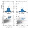 |
Fig. 1 Properties of the analyzed sample from the ALHAMBRA catalog. a) Best photometric redshift distribution, b) stellar mass distribution, c) mass versus isophotal area relation, and d) color (mF365W−mF582W) versus stellar mass diagram. Gray symbols correspond to the total ALHAMBRA sample. Dashed histograms and open circles correspond to our initial sample, and blue histograms and symbols correspond to our final sample of 29 early-type galaxies after quality control cuts. The dashed black line represents the arbitrary red sequence-blue cloud division at mF365W−mF582W < 1.7. |
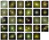 |
Fig. 2 Color images of the 29 massive early-type galaxies analyzed in this paper. Each image corresponds to 22′′ × 22′′ centered on each target. The number of each image corresponds to the ID from Table A.1. |
3. Method
The method used in the analysis can be summarized in four main steps: the homogenization of the point-spread function (PSF), the spatial binning of each object, the determination of the different stellar populations through the SED fitting of each bin, and finally, the representation of the 2D maps. The homogenization of the PSF ensures a homogeneous photometry. The spatial binning technique used in the analysis is the centroidal Voronoi tessellation. For the SED fitting, we used the MUFFIT code (MUlti-Filter FITting in photometric surveys; Díaz-García et al. 2015). In this section we describe each step in detail.
3.1. PSF homogenization
One of the challenges faced by data management of current large surveys is to provide homogeneous photometry and morphology for a large number of objects over large areas of the sky. To perform good-quality multicolor photometry, it is necessary to sample the same physical region of the galaxy taking into account the smearing produced by the different PSFs of each filter. These PSF variations may produce artificial structure that could bias our results (Bertin 2011). To avoid this problem, we have developed a method to analyze, characterize, and homogenize the PSF using the code PSFEx (Bertin 2013).
We first analyze the seeing of every image and choose a target PSF for the homogenization. The algorithm allows the user to choose the target PSF of the analyzed images. For this specific case, the worst (widest) PSF value of the image set was chosen for the homogenization. After selecting the target PSF, we generate a homogenization kernel that depends on the image position by running SExtractor (Bertin & Arnouts 1996) and PSFEx (Bertin 2013) in every image. To generate the homogenization kernel, PSFEx performs a χ2 minimization to fit the target PSF. A 2D Moffat model is used as an homogenization kernel. After determining the variable PSF models, we convolve each image with its corresponding kernel using a fast Fourier transform (FFT). Although the method penalizes computer resources, it increases the speed of the process in large images. The homogenization process allows image combinations and photometry measurements to be more consistent at the expense of degrading some images. Therefore it is important to apply the method to a set of images with similar quality. Finally, we need to take into account that the homogenization process has consequences in the image noise, producing pixel-by-pixel correlations. To correct for this, the algorithm recalculates the noise model of the images following the procedure described in Labbé et al. (2003) and Molino et al. (2014). For square apertures of different areas, the algorithm makes a high number of measurements of the sky flux in each aperture. The side of each square aperture varies from 2 to 30 pixels. A Gaussian fit is made to the resulting histogram, and the sky noise in an aperture of N pixels is modeled. Using apertures at different locations on the images, but also different aperture sizes, we account for the pixel-by-pixel correlation. This recalculated noise model has been used for computing the photometric errors.
3.2. Centroidal Voronoi tessellation
Spatial binning is a widely used technique to reach a required minimum S/N for a reliable and unbiased extraction of information. Given the large variations in the S/N across the detector, ordinary binning and smoothing techniques are not suitable to capture detailed structure. Cappellari & Copin (2003) tested different methods of adaptively binning IFS data and concluded that the centroidal Voronoi tessellation (CVT) is the optimal algorithm that solves the 2D binning problems. We used this binning scheme that adapts the size of the bin to the local S/N (e.g., larger bins were applied in regions with a low S/N, while a higher resolution was retained in parts with a high S/N). Following their prescription, we extended the adaptive spatial binning of IFS data proposed to photometric imaging data.
Before the CVT, a mask was applied to determine the area of the object to be analyzed. When the area is too small, we lose information of the outskirts. When the area is too large, it includes regions with low S/N and the tessellation will not satisfy the morphological and uniformity requirements in the outer parts. Neither situation will produce an optimal tessellation, therefore we need to reach a compromise between the resolution and the S/N achieved. All pixels inside the Kron radius of filter F365W, RKron, were selected for the CVT. RKron is defined by SExtractor as a flexible elliptical aperture that confines most of the flux from an object and has been empirically tested to enclose >90% of the object light. When secondary objects were present in the image, they were masked to avoid contaminating light. An area of 1.5 Reff of each secondary objects was masked during the analysis. Reff is defined as the half-light radius, that is, the radius containing 50% of the object light. Reff was always defined from the synthetic F814W images created to emulate the analogous band of the Advanced Camera for Surveys (ACS) onboard the Hubble Space Telescope (HST). These images are created as a linear combination of individual filter images and are used in ALHAMBRA for detection and completeness purposes (Molino et al. 2014).
The CVT algorithm is divided into three different phases:
-
Phase I: Accretion phase.
-
(i)
Start the first bin from the highest S/N pixel of the image.
-
(ii)
Evaluate the mass centroid of the current bin.
-
(iii)
Select a next pixel as candidate to be included in the current bin and analyze the following conditions:
-
(a)
the candidate pixel is adjacent to the current bin;
-
(b)
the roundness (Rc) of the bin would remain smaller than 0.3, where
 , rmax is the
maximum distance between the centroid of the bin and any of the
bin pixels, and rref is the
radius of a disk of the same area as the whole bin;
, rmax is the
maximum distance between the centroid of the bin and any of the
bin pixels, and rref is the
radius of a disk of the same area as the whole bin; -
(c)
the potential new bin S/N would not deviate from the target S/N by more than the current bin.
-
(a)
-
(iv)
Complete the addition of pixels to the current bin and start a new bin from the unbinned pixel closest to the centroid of the last bin. Return to step (ii) until all pixels are processed as successful and added to a bin or as unsuccessful and classified as unbinned.
-
(i)
-
Phase II: Reassigning phase.
-
(v)
Evaluate the mass centroid of all the successful identified binsand reassign the unsuccessfully binned pixels to the closest of thesebins.
-
(vi)
Recompute the centroid of each final bin.
-
(v)
-
Phase III: Equi-mass CVT.
-
(vii)
Use the previous centroids as initial generators to perform aVoronoi tessellation.
-
(viii)
Determine the mass centroids of the Voronoi regions according to ρ = (S/N)2 to force-generate bins that enclose equal masses according to that density. Use this new set of centroids as new generators.
-
(ix)
Iterate over step (vii) until the old and the new generators converge.
-
(vii)
This optimal binning scheme satisfies the following requirements: a) topological requirement: a partition without overlapping or holes, b) morphological requirement: the bins have to be as compact as possible so the best spatial resolution is obtained along all directions, c) uniformity requirement: small S/N scatter of the bins around a target value, to avoid compromising the spatial resolution in order to increase the S/N of each bin, and d) equal-mass bins according to a density distribution of ρ = (S/N)2.
When we consider the photometric depth of the ALHAMBRA images and the characteristic SED of typical early-type galaxies, the S/N will vary significantly from filter to filter and even along different redshifts. According to Díaz-García et al. (2015, see their Fig. 7), the bluest filter, F365W, is on average the band with the lowest S/N at redshift z < 0.4. Therefore, F365W will place constraints in our ability to determine reliable stellar population parameters. Enforcing a minimum S/N in filter F365W will ensure a proper S/N in the remaining bands and also a reliable determination of stellar parameters. In order to obtain typical uncertainties of Δlog AgeL = 0.14 and Δ[Fe/H]L = 0.20 for z < 0.4 in ALHAMBRA red-sequence galaxies, the SED fitting code used, MUFFIT, requires an S/N ~ 6 in the bluest filter, F365W. For a more detailed discussion of the effect of different S/Ns on the derived stellar population parameters, we refer to Sect. 4.2 of Díaz-García et al. (2015). To be conservative, CVT was performed in the filter F365W where the target S/N was set to 10, defined as the average S/N of the bins. The tessellation was then applied to the images in all the filters, and finally, the photometry of every region in all the filters was determined.
Although ALHAMBRA images are already background subtracted, this subtraction was applied globally over the entire image. We performed a local sky subtraction considering an area of 100 × 100 pixels (22′′ × 22′′) around each target galaxy. Assuming the small area subtended in the sky by each object, we considered as a first approximation a constant sky subtraction. A second approach was tested by applying CHEF functions (Jiménez-Teja & Benítez 2012). This tool models the light distribution of the galaxy through an orthonormal polar base that is formed by a combination of Chebyshev rational functions and Fourier polynomials. We note that no significant improvement was detected, therefore we finally applied a constant sky subtraction.
3.3. Stellar population parameters
After the CVT was performed and the photometry of every region in every filter was determined, we ran the code MUFFIT to obtain 2D maps of different stellar populations properties. MUFFIT is a generic code optimized to retrieve the main stellar population parameters of galaxies in photometric multi-filter surveys. The code compares the multi-filter fluxes of galaxies with the synthetic photometry of mixtures of two single stellar populations (SSP) for a range of redshifts and extinctions through an error-weighted χ2 approach. In addition, the code removes during the fitting process the bands that are affected by emission lines in order to improve the quality of the fit. The determination of the best solution space is based on a Monte Carlo method. This approach assumes an independent Gaussian distribution in each filter, centered on the band flux or magnitude, with a standard deviation equal to its photometric error. Each filter is observed and calibrated independently of the remaining filters, so that the errors of different filters are not expected to correlate. This approach not only provides the most likely range of ages, metallicities (both luminosity- and mass-weighted), extinctions, redshifts, and stellar masses, but sets constraints on the confidence intervals of the parameters provided.
Several studies have shown that the mixture of two SSPs is a reasonable compromise that significantly improves the reliability of determining the stellar population parameters of multi-filter galaxy data (Ferreras & Silk 2000; Kaviraj et al. 2007; Lonoce et al. 2014). Rogers et al. (2010) showed that the mixture of two SSPs is the most reliable approach to describe the stellar population of early-type galaxies. Most recently, López-Corredoira et al. (2017) fit a set of 20 red galaxies with models of a single-burst SSP, combinations of two SSPs, and an extended star formation history. They concluded that exponentially decaying extended star formation models (τ-models) improve the fits slightly with respect to the single-burst model, but they are considerably worse than the fits based on two SSPs, further supporting the residual star formation scenario. Based on these studies, we considered the two-SSP model-fitting approach the best method for our study. However, MUFFIT is currently being tested with later-type galaxies, and future versions of the code will also account for the use of different sets of SSPs or τ-models for the best choice of the user. MUFFIT has been tested and verified using data from the ALHAMBRA survey (Moles et al. 2008). In particular, MUFFIT accuracy and reliability tests are performed considering the ALHAMBRA sensitivity and filter set, which means that the analysis and results presented in Díaz-García et al. (2015) are directly applicable to our study here.
Single stellar population models are a key ingredient to distinguish the physical properties of stellar populations. We provide MUFFIT with two different sets of SSP models: BC03 (Bruzual & Charlot 2003), and E-MILES (Vazdekis et al. 2016). To explore any potential dependence of the SSP model used, the analysis of this study was performed using both sets of models. For BC03 with a spectral coverage from 91 Å to 160 μm, we selected ages up to 14 Gyr, metallicities [Fe/H] =−1.65, −0.64, −0.33, 0.09, and 0.55, Padova 1994 tracks (Bressan et al. 1993; Fagotto et al. 1994a,b; Girardi et al. 1996), and a Chabrier (2003) initial mass function (IMF). E-MILES provides a spectral range of 1680–50 000 Å at moderately high resolution for BaSTI isochrones (Pietrinferni et al. 2004). E-MILES models include the Next Generation Spectral Library (NGSL, Heap & Lindler 2007) for computing spectra of single-age and single-metallicity stellar populations in the wavelength range 1680–3540 Å, and the NIR predictions from MIUSCATIR (Röck et al. 2015). For the BaSTI isochrones, we chose 21 ages in the same age range as BC03, but with metallicities [Fe/H] =−1.26, −0.96, −0.66, −0.35, 0.06, 0.26, and 0.4. We assumed a Kroupa universal-like IMF (Kroupa 2001). MUFFIT allows the user to choose among several extinction laws. We used the Fitzpatrick reddening law (Fitzpatrick 1999) throughout, with extinctions values Av in the range of 0 and 3.1. This extinction law is suitable for dereddening any photospectroscopic data, such as ALHAMBRA (further details in Fitzpatrick 1999).
To minimize the free fitting parameters, we provide MUFFIT with an initial constraint of redshift values. We used the spectroscopic redshifts determined by SDSS (Gallazzi et al. 2005) as input parameter. When spectroscopic redshifts were not available, photometric redshifts determined by ALHAMBRA (Molino et al. 2014) were used. We note that MUFFIT linearly averages the ages and metallicities (their Eqs. (16) and (17)) (log ⟨Age⟩and log ⟨[Fe/H]⟩ versus ⟨log Age⟩ and ⟨log[Fe/H]⟩)2. Both types of averaging are found in the literature (e.g., MaNGA versus CALIFA). We note that a logarithmic weighting formalism may give more weight to younger and metal poorer stellar populations. Owing to the small range in age and [Fe/H] that we cover in our analysis, no significant consequences are introduced in the analysis because of differences in the mathematical treatment. Therefore both approaches are expected to lead to similar results.
3.4. 2D Maps: age, [Fe/H], and Av
MUFFIT provides luminosity- and mass-weighted ages, metallicities, and extinctions. Mass-weighted properties trace the whole evolutionary history of the galaxy better since they give insight into its mass assembly history. On the other hand, luminosity-weighted properties are more sensitive to the most recent periods of star formation in the galaxy. Throughout this study, we show both mass-weighted (log AgeM and [Fe/H]M) and luminosity-weighted (log AgeL and [Fe/H]L) properties as a way to complement each other and identify certain processes more clearly. As an illustrative example, Fig. 3 presents the age, metallicity, and extinction maps and radial profiles (see Sect. 5) of a galaxy using E-MILES models and luminosity-weighted properties. We note a very distinct region around (ΔX, ΔY) = (−5, −5) with a younger, more metal-poor, and more extinct stellar population than the rest of the galaxy. To further probe the quality of the SED fits, the χ2 map of every object is inspected as a goodness-of-fit quality check. A detailed definition of the error-weighted χ2 minimization process can be found in Sect. 3.2.1 of Díaz-García et al. (2015). We note that although generally speaking, a value of χ2 ~ 1 is a mean value for a good fit, χ2 serves only as an indicator. Other parameters must also be examined as the distribution of residuals. A good model fit should yield residuals that are normally distributed around zero with no systematic trends. Figure 4 shows the χ2 map of the example object. Visual inspection of the SED does not show evidence of higher photometric errors that could suggest an artificial feature, although the χ2 of the fits in that area are slightly higher than the median value. A detailed light decomposition of our sample will reveal the nature of these substructures and will be present in future studies. The 2D maps as well as the radial profiles of all the sample objects are provided in Appendix C.
4. Integrated versus resolved properties of the sample
In addition to the multi-filter photometry of every bin in a galaxy tessellation, we also determined the integrated stellar properties of each galaxy. This integrated photometry was obtained using exactly the same method as described in Sect. 3 for the galaxy as a whole, with no tessellation, emulating integrated aperture photometry. Several studies point out that in addition to the uncertainties in the stellar properties inferred from all uncertainties in the model assumptions, there are additional biases related with the fitting procedure that can affect the determination of integrated stellar population parameter. In particular, the outshining bias, that is, young stellar populations obscuring older stellar components behind their bright flux, could produce a missing mass effect (Zibetti et al. 2009; Sorba & Sawicki 2015). This problem is less severe when a resolved analysis is made, as these young components are localized in specific areas. Although we do not expect a strong contribution from young components in our sample of massive early-type galaxies, we analyze the differences obtained with both methods here.
Figure 5 compares for each galaxy the total stellar mass derived from the integrated method (log  ) with the mass obtained by adding the estimated masses in each tessellation bin (log
  ). The two values agree very well, with a mean difference of –0.0 ± 0.07 dex for BC03 and –0.01 ± 0.03 dex for E-MILES.
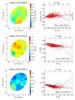 |
Fig. 3 Luminosity-weighted stellar population properties maps and radial profiles analyzed using E-MILES-based models for the example object 81461302615. Left column: 2D maps for log Age, [Fe/H], and Av covering an area of 22′′ × 22′′ around the target galaxy. The color range has been chosen to highlight inhomogeneities. Right column: log Age, [Fe/H], and Av as a function of the circularized galactocentric distance R′ (see Sect. 5). Each red circle corresponds to a bin in the 2D map. The black dashed line corresponds to the error-weighted linear fitting. Black crosses correspond to outliers identified during the sigma-clipping process and were not considered during the fit. |
Figure 6 compares the Age and [Fe/H] from the integrated photometry to the weighted mean properties (⟨Age
 and ⟨[Fe/H]) from the spatially resolved analysis. The spatially resolved weighted mean properties are defined as
 ![Mathematical equation: \begin{eqnarray} \label{eq:1} &&\langle \mathrm{Age} \rangle_{\rm L}^{\rm resolved} = \frac{{\sum_{i} L_{\mathrm{5515},i}\cdot \mathrm{Age}_{\mathrm{L},i}}}{{\sum_{i} L_{5515,i}}}, \text{and} \\\label{eq:2} &&\langle\mathrm{[Fe/H]}\rangle _{\rm L}^{\rm resolved} = \frac{{\sum_{i} L_{5515,i}\cdot \mathrm{[Fe/H]}_{\mathrm{L},i}}}{{\sum_{i} L_{5515,i}}} , \end{eqnarray}](/articles/aa/full_html/2018/01/aa30313-16/aa30313-16-eq72.png) where L5515,i is the luminosity of bin i evaluated at a reference rest-frame wavelength of 5515 Å and AgeL,i and [Fe/H] L,i the luminosity-weighted age and metallicity for that i bin.
where L5515,i is the luminosity of bin i evaluated at a reference rest-frame wavelength of 5515 Å and AgeL,i and [Fe/H] L,i the luminosity-weighted age and metallicity for that i bin.
Once again, the values are in agreement with no significant offset (Δlog AgeL,BC03 = −0.02 ± 0.15, Δlog AgeL,EMILES = −0.02 ± 0.05, Δ[Fe/H]L,BC03 = 0.03 ± 0.07, Δ[Fe/H]L,EMILES = 0.03 ± 0.08). Results are shown for both SSP models. Overall, the total stellar mass, age, and metallicity estimated from integrated photometry are remarkably robust when compared with those from a spatially resolved analysis. Similar conclusions (see Fig. B.1) are reached when mass-weighted mean properties are evaluated where the mass-weighted version of Eqs. (1) and (2) are applied (see Appendix B). These results agree with the recent conclusion obtained using CALIFA galaxies (González Delgado et al. 2014, 2015) where galaxy-averaged stellar ages, metallicities, mass surface density and extinction are well matched by the corresponding values obtained from the analysis of the integrated spectrum. Table A.1 summarizes the spatially resolved stellar properties of the sample and the median χ2 of the SED fits.
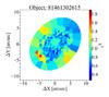 |
Fig. 4 Goodness-of-fit map, χ2, for the example object 81461302615. |
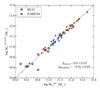 |
Fig. 5 Integrated versus spatially resolved stellar masses derived from MUFFIT for the 29 massive early-type galaxies analyzed in this paper. Both BC03 and E-MILES SSP models were used. Symbols enclosed in squares indicate the six peculiar cases analyzed in Sect. 5.1. A normal distribution has been fit to the difference between the x-axis and the y-axis. The mean and standard deviation is labeled as Δ. The black dashed line shows the one-to-one relation. |
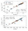 |
Fig. 6 Integrated versus spatially resolved ages and metallicities derived from MUFFIT for the 29 massive early-type galaxies analyzed in this paper. Both BC03 and E-MILES SSP models were used. Symbols enclosed in squares indicate the six peculiar cases analyzed in Sect. 5.1. A normal distribution has been fit to the difference between the x-axis and the y-axis. The mean and standard dispersion is labeled as Δ in each panel. The black dashed line shows the one-to-one relation. |
 |
Fig. 7 Spatially resolved ages and metallicities versus mass. The lines indicate the relation obtained in Gallazzi et al. (2005), where the solid line corresponds to the median distribution and the dashed lines to the 16th and 84th percentiles. Symbols enclosed in squares indicate the six peculiar cases analyzed in Sect. 5.1. |
4.1. Spatially resolved mass-age and mass-metallicity relations
Galaxies in the local Universe exhibit a clear correlation between stellar mass and their properties in the well-known mass-age and mass-metallicity (MZR) relations. Instead of characterizing the nature of these relations, we wish to determine how well our spatially resolved mass-age and mass-metallicity relations follow previous trends to guarantee that our technique is able to reproduce previous observational evidence.
In Fig. 7 we show the relation between the spatially resolved age and metallicity with the mass, assuming both SSP models. For comparison purposes, we have overplotted the relation obtained by Gallazzi et al. (2005), which includes all types of galaxies. Gallazzi et al. (2005) used a Bayesian approach to derive ages and metallicities by a simultaneous fit of five spectral absorption features. Their analysis used absorption line indices with different sensitivities for age and metallicity, focusing on Lick indices and the 4000 Å break (Gorgas et al. 1993; Worthey et al. 1994). The population properties were determined using BC03 SSP models. The ages of our galaxies show a clear increase with the galaxy mass, thus, more massive galaxies tend to be older, which represents the well-known mass-age relation. Although this trend overall follows the mass-age relation obtained by Gallazzi et al. (2005) for massive galaxies, there are five low massive galaxies for each SSP (log M⋆< 11.0) that significantly depart from the general trend. These outliers are identified as either star-forming galaxies or AGN candidates (see Sect. 5.1 for further details). Peng et al. (2015) split the galaxy population used by Gallazzi et al. into quiescent and star forming and found a different mass-age relation between the two populations. The observational evidence found by Peng et al. (2015) would explain the position of our star-forming galaxies outside the general trend. Figure 7 shows that the spatially resolved stellar population properties derived from this method reproduce the well-known downsizing effect (Cowie et al. 1996).
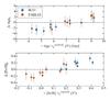 |
Fig. 8 Difference stellar population values between our study and SDSS (Gallazzi et al. 2005) as a function of AgeL (top panel) and [Fe/H]L (bottom panel) from this study. Photometric values of our analysis were determined in the same aperture size as SDSS (3′′). The black dashed line shows the one-to-one relation. |
On average, the global metallicities of the galaxies increase with their mass (bottom panel in Fig. 7) and agree with the general trend found by Gallazzi et al. (2005). Peng et al. (2015) also found a different metallicity-mass relation between quiescent and star-forming galaxies. At a given stellar mass, the stellar metallicity of quiescent galaxies is higher than for star-forming galaxies for log M⋆ < 11. According to their Fig. 2 and for our mass range, the metallicity difference for the two galaxy populations would be [Fe/H] ~−0.2 dex, in agreement with our BC03 results. In general, the behavior of our galaxy sample reproduces the mass-age and mass-metallicity relations of the local Universe well based on SDSS observations, although a clear offset is present based on the SSP models used.
4.2. Comparison with previous spectroscopic studies
No common objects were found between our sample and any IFU survey such as SAURON, CALIFA, or MaNGA. This inconvenience hinders a one-to-one galaxy comparison of our method. However, there is a subsample of nine galaxies in the SDSS catalog for which individual integrated spectroscopy is available. Estimates of ages and metallicities of the central area of these galaxies are provided by Gallazzi et al. (2005). SDSS spectra were taken using a fiber aperture of 3′′, while our photo-spectra are not restricted to a fixed aperture. For a fair comparison and to avoid any aperture effects, we considered only the spatially resolved properties of our maps in a 3′′ circular aperture placed at the galaxy center (⟨Age (3′′) and ⟨[Fe/H] (3′′)).
Figure 8 presents a one-to-one comparison of the spectroscopic luminosity-weighted ages and metallicities given by Gallazzi et al. (2005) and our photometric values analyzed in a 3′′ aperture of the subsample of nine common objects (ΔAgeL = ⟨Age (3′′) – AgeL(SDSS) and Δ[Fe/H] = ⟨[Fe/H] (3′′) – [Fe/H]L (SDSS)). The offsets between both studies are plotted against the luminosity-weighted age and metallicity to explore any dependency. A careful look at the top panel reveals that except for one single object that drives a misleading trend, the sample shows an offset for BC03, in agreement with the expected ~2 Gyr difference determined by Díaz-García et al. (2015). As the authors concluded, this discrepancy is due to intrinsic systematic differences between the two methods. In the bottom panel, an apparent trend is shown between the metallicity offsets as a function of the luminosity-weighted metallicities, suggesting a possible degeneracy. In order to study the accuracy and reliability of the stellar population parameters retrieved, we quantify the expected degeneracies among the derived parameters in the next section.
4.3. Degeneracies
Understanding the degeneracies between the different parameters is a crucial step in order to avoid any misinterpretation that could misdirect the analysis. Although some of these degeneracies are unavoidable, in this section we analyze their extension and potential effects. As in any color-dependent diagnostic technique, any parameter that can modify the color of the object needs to be evaluated. This means that we need to include not only the age and metallicity, but also the extinction in the analysis of the degeneracies. To address the degeneracy problem, we used the stellar population values recovered by MUFFIT during the Monte Carlo approach for every single object in every bin of the tessellation. Then we stacked each distribution to build a final distribution per object and obtained distributions among pairs of parameters (age, metallicity, and extinction). To quantify the final degeneracy between each pair of distributions, we followed the method used in Díaz-García et al. (2015). Each distribution of potential values is characterized by setting confidence ellipses (2D confidence intervals) that enclose the results provided during the Monte Carlo process. These ellipses are obtained from the covariance matrix of each distribution. The ellipticity, e, and the position angle, θ, of these ellipses allow us to quantify the degeneracies. A value of e close to zero implies no degeneracy between the two parameters. Furthermore, when θ lies on any of the two axes (θ is a multiple of π/2), the two parameters are not correlated and no degeneracy is found. In addition, Díaz-García et al. (2015) quantified the level of degeneracy between parameters via the Pearson correlation coefficient (see Eq. (25) in Díaz-García et al. 2015). If the Pearson coefficient, rxy, is close to 1 (or −1), the correlation (anticorrelation) is large, meaning that there is a degeneracy between the parameters. In contrast, the closer the coefficient is to 0 (e.g., −0.1 ≤ rxy ≤ 0.1), the more uncorrelated are the parameters. Thus, we finally have an ellipse of degeneracy (e, θ and rxy) per object for every pair of parameters, where the ellipse represents the covariance error ellipse that encloses, at the 95% confidence level, the distribution of the parameters during the Monte Carlo approach.
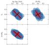 |
Fig. 9 Stacked covariance error ellipses, at the 95% confidence level, of the stellar population parameters for all the objects in the sample. The red lines illustrate the minor and major axis of each ellipse, while the black lines correspond to the median values for the entire sample for E-MILES models. |
Figure 9 corresponds to the stacking of the ellipses of degeneracy for all the objects, where the red lines illustrate the minor and major axis of each ellipse and the black lines show the median values for the entire sample. Figure 10 provides the histogram of θ, e, and rxy in all regimes. Table 1 summarizes the median values of the covariance error ellipses. An old metal-rich sample such as ours exhibits an anticorrelation in all cases. This means that, for example, a stellar population reddened by extinction can imitate the behavior of a population that is reddened because of the metal-rich content, or vice versa. We also checked that the general degeneracy trends do not significantly vary on the basis of the input model set (BC03 vs. E-MILES) except for the case of log AgeM vs. [Fe/H]M where E-MILES SSP can break or reduce the degeneracy (rxy = –0.10). We emphasize that these results are restricted to our sample, that is, to early-type galaxies, and that the covariance error ellipses for more complicated stellar population histories could be different.
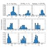 |
Fig. 10 Histogram of the position angle (θ), ellipticity (e), and Pearson’s coefficient (rxy) for E-MILES models. The related variables are shown at the top of each column. |
Median values of the covariance error ellipses for all the objects in the sample: position angle (θ), ellipticity (e), and Pearson’s coefficient (rxy).
5. Radial profiles and gradients
To show and quantify radial variations of the galaxies, we obtained the radial profiles of the three parameters (age, metallicity, and extinction) for all 29 galaxies. It is common practice to derive radial profiles of stellar population properties by binning the output values into elliptical annuli that are scaled in along the major axis such that the bins are constant in effective radius. These azimuthally averaged radial profiles assume a priori symmetry in the stellar population of the galaxies and remove the important 2D information imprint in the maps by directly collapsing the information to a 1D plot. We take a different approach by plotting the stellar population values of each bin in each object as a function of the circularized galactocentric distance, R′: 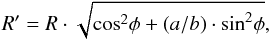 (3)where R is the galactocentric distance of the bin, φ is the angle of the bin with respect to the semi-major axis, and a/b is the semi-axis ratio of the galaxy as obtained by IRAF/Ellipse in the synthetic F814W band. Along the semi-major axis, (φ = 0) R′ = R, whereas in a more general case, R′ ≥ R. For the specific case of an apparent circular galaxy (a/b = 1), R′ = R at all φ. This parameter, R′, allows us to take the information in all the bins into account while considering the morphology of the object. The right panels in Fig. 3 present the radial profiles for the age (log Age), metallicity ([Fe/H]), and extinction (Av) as obtained from the 2D maps of an example object. Each red symbol corresponds to a bin in the 2D map. For a given R′, the spread of the values gives us an idea of the departure of the stellar population from symmetry. It is important to note that the majority of previous studies cannot reach beyond R = 1.5 Reff, except for CALIFA (González Delgado et al. 2015), which reaches 2.7 Reff. In contrast, our analysis derives gradients out to 2−3.5 Reff.
Although the radial profiles of our sample seem to follow, in general, linear relations as a function of galactocentric distance, several authors have assumed power-law gradients. For comparison purposes, radial gradients were fitted assuming a linear relation in linear space and logarithmic space as  where ∇X corresponds to the radial gradient of the different stellar population analyzed (in linear scale ∇log Age (dex/Reff), ∇[Fe/H] (dex/Reff), and ∇Av (mag/Reff) and in log scale ∇log Age (dex/dex), ∇[Fe/H] (dex/dex), and ∇Av (mag/dex) and X0 the fitted values at the central region (log Age0, [Fe/H]0, and Av0) for the case of luminosity-weighted values and mass-weighted values. Radial gradients were determined through an error-weighted linear fitting of the profiles out to 2−3.5 Reff (depending on the photometric depth of each object). The process was performed iteratively via a sigma clipping on the residuals to remove outliers. Black crosses in Fig. 3 represent values that were not considered during the fit. The black dashed line corresponds to the final gradient. The individual uncertainties of each stellar population value of each region are derived by MUFFIT through a Monte Carlo method. For clarity we did not include individual errors in the figure, but typical errors are Δlog Age = 0.15 dex, Δ[Fe/H] = 0.15 dex, and ΔAv = 0.10 mag. The gradients determined for each object are summarized in Table A.2. The radial profiles and the 2D maps of all the sample objects can be found in Appendix C.
5.1. Peculiar cases
Although it is beyond the scope of this paper to enter in the peculiarities of individual objects and maps, it is worth mentioning that the level of resolution is so high in some cases that a simple visual inspection of the maps reveals fine structures. In this section, we describe the peculiar cases that stand out from the analyzed sample. The 2D maps and the radial profiles of all the sample objects can be found in Appendix C.
-
AGN profiles: Galaxies 81422406945 (Fig. C.5), 81451206302 (Fig. C.11), and 81473103857 (Fig. C.24) show very distinct profile behaviors that are different from those of the remaining sample. With a very well-defined core, their radial profiles are not well represented by a linear fitting. Objects 81451206302 and 81422406945 were previously identified as AGN candidates based on their X-ray detection (Flesch 2016; Page et al. 2012). The source 81473103857 seems to be an obscured AGN (Cutri et al. 2002, 2003). Similar core profiles have previously been observed in several studies (Koleva et al. 2011; Li et al. 2015). Some of the CALIFA spheroidal galaxies also show positive central gradients in age (González Delgado et al. 2014, 2015). It is likely that these very young areas with high extinction levels are due to the AGN and not to the properties of the underlying stellar population.
-
Disk or ring substructures: Galaxy 81422406945 (Fig. C.5) shows an apparent disk that is particularly evident in metallicity along the major axis. As mentioned before, this object has been identified as an AGN candidate. Galaxies 81473405681 (Fig. C.13) and 81422407693 (Fig. C.22) show apparent rings more prominent in age. A detailed light decomposition of these objects will reveal the nature of these substructures.
-
Very young profiles: In addition to two of the AGN profiles (81451206302 and 81473103857) and the objects with apparent rings (81473405681 and 81422407693) mentioned before, one other galaxy also has a very young profile (81474307526, Fig. C.16). These five galaxies correspond to the blue objects outside the red sequence in Fig. 1 (panel d). These objects are star-forming galaxies or AGNs, based on their location in panel d of Fig. 1.
In order to avoid compromising the results, we excluded these six objects with peculiar profiles from the following analysis. However, considering that the main goal of this study is to present and test our method, we included the profiles, maps, and spatially resolved properties in the final tables and appendices as a probe of the potential of the method.
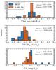 |
Fig. 11 Histograms of the linear space gradients for log AgeL (upper panel), [Fe/H]L (middle panel), and Av (bottom panel) for different SSP models. The median μ values are labeled in each panel. The six objects with peculiar profiles (Sect. 5.1) have been removed from the analysis. |
Median light-weighted and mass-weighted gradients in linear and logarithmic space.
5.2. Radial gradients
The age, metallicity, and extinction luminosity-weighted gradients in linear space are summarized in the histograms of Fig. 11. Mass-weighted stellar population gradients are shown in Fig. B.2. In order to avoid compromising the results, we excluded the peculiar cases from the analysis (see Sect. 5.1) for a final subsample of 23 objects. Table 2 presents the median light- and mass-weighted values of the linear and logarithmic space radial gradients. Although the median values do not seem to be affected by which SSP model is used, BC03 produces a higher scatter driven by a few relatively large outliers. This evidence indicates that systematic errors are associated with the different SSP models.
Comparison table providing the most relevant previous studies on stellar population gradients.
5.2.1. Age gradients
Our sample of early-type galaxies has, on average, flat age gradients with a median of ∇log AgeL = 0.02 ± 0.08 dex/Reff, and ∇log AgeL = 0.02 ± 0.06 dex/Reff for BC03 and E-MILES, respectively. As seen from Table 2 and Fig. 11, none of the input SSP models used during the analysis causes significant differences in the median gradients, although BC03 produces some outliers. It is also remarkable how similar the luminosity- and mass-weighted values are. This suggests that galaxies, on average, behave similarly on mass and on light and that the half-mass radius (RMLR) and half-light radius (Reff) on early-type galaxies should be similar. This result suggests that the contribution of the second SSP (the younger component) is small and the star formation history of our early-type population is well represented by mainly an old SSP component. This result agrees with a previous CALIFA analysis (González Delgado et al. 2014), which found the ratio for early-type galaxies to be RMLR/Reff ~ 0.9. However, our results differ from a recent MaNGA analysis. Goddard et al. (2017) found a marked difference between luminosity- and mass-weighted age gradients where the mass-weighted median age does show some radial dependence with positive gradients at all galaxy masses. A more detailed study of mass-to-light (M/L) maps and gradients of different galaxy type will be performed in future works.
To place our results in context with the literature and provide a quantitative comparison, Table 3 summarizes the most relevant previous studies on stellar population gradients in early-type galaxies. The list combines a wide variety of different observational approaches, sample sizes, and radial coverage. The radial coverage varies between 1 and 2 Reff except for the photometric studies, which reach farther galactocentric distances. The distribution of the gradients derived in these studies are visualized in Fig. 12. Most studies in the literature have found either a flat or slightly positive age gradients, except for the CALIFA inner gradient result. González Delgado et al. (2015), using CALIFA galaxies (~41 early-type), found very negative inner (<1 Reff) gradients (~–0.25) that become flat at larger galactocentric distances. Our results agree with previous long-slit analyses of early-type galaxies (e.g., Mehlert et al. 2003; Wu et al. 2005; Reda et al. 2007; Spolaor et al. 2010) and also with the most recent IFU studies (e.g., Rawle et al. 2008, 2010; Kuntschner et al. 2010; Wilkinson et al. 2015; Goddard et al. 2017), in particular regarding the lack of a significant age gradient. With a median age gradient value of 0.0 dex/Reff and 0.03 dex/dex, our results agree very well with previous studies.
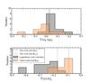 |
Fig. 12 Distribution of age and metallicity gradients for early-type galaxies obtained in previous studies. All values have been taken from Table 3. The dashed lines represent the stellar population gradients obtained in this work. |
5.2.2. Metallicity gradients
The vast majority of our galaxies have negative metallicity gradients, as expected in most of the galaxy formation scenarios. Although different notations are used to indicate metallicity ([Fe/H], [M/H] or [Z/H]), all the notations are directly comparable for solar-scaled models. Throughout this paper, we maintain the metallicity and gradient metallicity notation of the original study. The median gradients of our sample are ∇[Fe/H]L/Reff = −0.11 ± 0.07 dex/Reff for BC03 and ∇[Fe/H]L/Reff = −0.09 ± 0.06 dex/Reff for E-MILES. When we use logarithmic scale values for comparison purposes, we obtain ∇[Fe/H]L/log (R/Reff) = −0.20 ± 0.27 dex/dex and ∇[Fe/H]L/log (R/Reff) = −0.17 ± 0.13 dex/dex for BC03 and E-MILES, respectively. Once again, none of the input SSP models used during the analysis make significant differences in the median gradients. In addition, luminosity- and mass-weighted gradients are remarkably similar. Goddard et al. (2017) found luminosity- and mass-weighted metallicities and their radial dependence to be indistinguishable with an average offset of ~0.05 dex, in agreement with our results.
The metallicity gradient distribution of previous studies (Fig. 12) shows a wide range of values from –0.16 to –0.42 with a median of –0.25 dex/dex. The light-weighted metallicity gradient found in the present study (–0.17 dex/dex and –0.09 dex/Reff) is at the shallower side, but well within the distribution. Most notably, the IFU studies of Table 3 agree well with our metallicity gradients.
5.2.3. Extinction gradients
The bottom panel of Fig. 11 shows a variety of extinction behaviors with a tendency of flat Av gradients. MaNGA early-type galaxies also have a very small amount of dust and show shallow, relatively flat radial profiles (Goddard et al. 2017). González Delgado et al. (2015) CALIFA sample of ellipticals also show negative Av gradients with an almost dust-free behavior at distances larger than 1 Reff. Unfortunately, the lack of previous extinction gradient studies does not allow for further comparison.
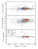 |
Fig. 13 Stellar population gradients AgeL, [Fe/H]L , and Av, in logarithmic space as a function of stellar mass. BC03 and E-MILES, SSP models have been included. Open circles correspond to Illustris simulation measurements in the outer (1–2 Reff) galaxy region (Cook et al. 2016). Dashed black lines show flat gradients. The six objects with peculiar profiles (Sect. 5.1) have been removed from the analysis. |
5.2.4. Correlation with mass
Figure 13 presents variations of stellar population gradients with the galaxy total mass. Total masses were calculated by adding the estimated mass in each tessellation bin (see Sect. 4). We overplot Illustris hydrodynamical simulation measurements in the outer galaxy region (1–2 Reff) from Cook et al. (2016). For comparison purposes, we overplot values obtained in logarithmic space and age gradients as ∇AgeL rather than ∇log AgeL. No clear correlation between total stellar mass and stellar population gradients is found for our mass range, in agreement with previous studies. González Delgado et al. (2014) also failed to find a clear trend between age gradients with mass for very massive spheroidal galaxies, although it seems that larger inner gradients occur in less massive galaxies (log M⋆< 11.2). The same behavior is found for metallicity gradients, where more massive galaxies tend to have weaker stellar metallicity gradients with no clear correlation. The MaNGA survey (Goddard et al. 2017) also failed to find a clear correlation between age and metallicity gradients with galaxy mass for massive early-type galaxies (log M⋆> 10.5). Overall, our results are compatible with those of the Illustris simulation, although our metallicity gradients are less steep than those of Illustris. Comparison with other studies shows that Illustris metallicity gradients (~–0.5 dex/dex) are steeper than the metallicity gradients from observations (see Table 3 and Fig. 12) and previous simulations (e.g., Kobayashi 2004; Hirschmann et al. 2015).
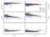 |
Fig. 14 Stacked radial profiles of log AgeL, [Fe/H]L, and Av. The left panels present the case of the E-MILES SSP models, and the right panels show the case of BC03. Gray open symbols correspond to the stellar population values of each individual bin in each spatially resolved object. Stars have been obtained by averaging the stellar population values of the sample in constant bins of 0.2 Reff between 0 ≤ R ≤ 3.6 Reff. The error bars are the standard deviation of the mean. When available, the profiles obtained by CALIFA (González Delgado et al. 2015) have been overplotted. MaNGA (Goddard et al. 2017) for early-type galaxies with log M⋆> 11.0 was also considered. The dashed black line corresponds to the best linear fit of the average stellar population values (stars). |
Stellar population gradients of the master radial profiles in linear and logarithmic space.
5.3. Master radial profile
Figures 14 and 15 show the age and metallicity (luminosity- and mass-weighted), and the extinction radial profiles obtained by stacking all the galaxies obtaining a master profile. We excluded the peculiar cases from the analysis (see Sect. 5.1) for a final subsample of 23 objects. The gray open symbols in each panel correspond to the individual bin in each spatially resolved object. The master profiles (star symbols) were obtained by averaging the stellar population properties of the sample in constant bins of 0.2 Reff between 0 ≤ R′ ≤ 3.5 Reff. The left panels in both figures correspond to E-MILES SSP models and the right panels correspond to BC03 SSP. The error bars represent the standard deviation of the mean. When available, the profiles obtained by CALIFA (González Delgado et al. 2014) are overplotted for the case of elliptical galaxies and the same BC03 SSP models as our study. Median stellar population parameters from MaNGA (Goddard et al. 2017) are also overplotted for the case of early-type galaxies with log M⋆> 11.0. Linear relations are fit to the master profiles. The gradients and the values at R′ = 0 are summarized in Table 4. Once again, the luminosity- and mass-weighted profiles show a similar behavior. We note again that while none of the input SSP models (BC03 versus E-MILES) make significant differences in the global profile, they do introduce a non-negligible offset between them.
We first remark that our profiles extend to larger galactocentric distances than any previous spectroscopic study. The reason is certainly that photometry is more sensitive than standard spectroscopy, although deeper photometry is needed to place stronger constraints on these outskirt areas. Overall, our stellar ages show flat profiles. A comparison with CALIFA shows remarkably similar radial gradients (flat ages) at R>Reff. Larger differences are found in the inner regions (R< 0.7 Reff). While our sample show a continuous flat profile, CALIFA galaxies present a negative age gradient only in these inner regions. Since the same input SSP models (i.e., BC03) are used in both studies, the different methods and techniques used are the main source to explain these discrepancies. The full spectral fitting of MaNGA uses the stellar population models of Maraston & Strömbäck (2011), which use the MILES stellar library. This means that although Figs. 14 and 15 compare MaNGA results with our results in both SSP models, in principle, the models of Maraston et al. would be more similar to E-MILES than to BC03. Our results are remarkably similar to MaNGA when E-MILES and mass-weighted properties are considered, and they slightly differ for the luminosity-weighted age gradient.
The stellar metallicity profiles show declining profiles at all radii, although our study shows slightly steeper gradients than those from CALIFA. Once again, our results are remarkably similar to MaNGA when similar SSP models are used. A larger sample and deeper photometry is needed for further analysis at larger galactocentric distances.
The stellar extinction behavior of the galaxies in our sample is consistent with a flat profile, which suggests that there are no significant changes in the dust content of early-type galaxies, and they show a constant Av = 0.2 mag at any given radius. MANGA early-type galaxies exhibit shallow relatively flat radial profiles with reddening values of E(B−V) ~ 0.05 for a similar mass range (Goddard et al. 2017). Considering Rv = Av/E(B−V) and assuming a value of Rv = 3.1, the MANGA extinction parameter is Av ~ 0.15, in good agreement with our results. In contrast, CALIFA galaxies show negative Av gradients out to R = 0.5 Reff with a dust-free behavior at larger distances, although absolute Av estimates of CALIFA are smaller than MANGA and our estimates.
In spite of the different technique used, the behavior of the radial variation of the different stellar properties is very similar in our multi-filter ALHAMBRA study and recent IFU studies. These results highlight the scientific power of our 2D multi-filter method. From this analysis, we can conclude that an average massive (~1011M⊙) early-type galaxy at a redshift z ~ 0.2 has a flat age gradient with an inner age of log Age0 ~ 0.93, and a negative metallicity gradient of ∇[Fe/H] ~−0.10 (dex/Reff) with an inner metallicity of [Fe/H]0 ~ 0.07.
6. Discussion and future work
Although the goal of this study is to explore the potential of IFU-like studies with multi-filter surveys, the successful results and the reasonable sample size allow us to shed some light on the formation history of galaxies in our sample. In this section, we compare our results with cosmological simulations and include some discussion of the prospects for extending our analysis in future works.
The most recent cosmological simulations propose a two-phase scenario for the formation of early-type galaxies: a first phase of dissipative processes (2 <z< 6) dominated by in situ star formation from inflowing cold gas (the monolithic-collapse scenario), and a second phase (0 <z< 2) where the galaxies grow through external accretion (mergers) and ex situ star formation (e.g., Domínguez-Tenreiro et al. 2006; Naab et al. 2009; Oser et al. 2012). The age and metallicity mean gradients can place constraint on the formation history of the galaxies as different formation models predict different gradients. In general, dissipative processes predict steep metallicity gradients, while merging scenarios predict shallower gradients because any pre-existing gradient is diluted (e.g., Kobayashi 2004; Pipino et al. 2008). However, different physical processes such as AGN feedback, SN feedback, young massive stars, or galactic winds can strongly influence the fraction of in situ formed stars versus accreted stars, and thus the overall gradients (Hirschmann et al. 2013, 2015). Gas-rich mergers with different degrees of dissipation have also been proposed as enhanced metallicity processes that will produce secondary star-formation events leading to steeper gradients (Kobayashi 2004).
Kobayashi (2004) successfully reproduced the formation and chemodynamical evolution of elliptical galaxies through SPH simulations. He found an average gradient of ∇log Z/log R = −0.3 dex/dex with a dispersion of ±0.2 in the local Universe. The metallicity gradients obtained in our study are considerably flatter than the values predicted by the dissipative-collapse models, thus major and minor mergers are expected to play a significant role for the assembly of these massive galaxies. With a median metallicity gradient of ∇[Fe/H]L = −0.17 ± 0.13 dex/dex, our study is in agreement with the predictions of Kobayashi (2004) of galaxies that have undergone major mergers.
In a more recent study, Hirschmann et al. (2015) investigated the origin of stellar population gradients in cosmological zoomed simulations of ten massive galaxies at large radii. The simulations followed metal cooling and enrichment from SN and AGB winds as well as galactic winds. At z ~ 0, galaxies have mean metallicity gradients of –0.35 dex/dex slightly steeper than our results. They explained the origin of these gradients as based on two components: on one hand, the accretion of metal-poorer stellar populations in major and minor mergers dilutes a pre-existing gradient (in situ gradient), on the other hand, re-infall of previously ejected metal-poor gas onto the galaxy, due to the galactic winds, could form metal-poor stars. Age gradients are in general mildly positive at z = 0 (⟨ ∇logAge⟩ = 0.04 dex/dex) because the ages of the accreted stellar population are older than those of the in situ formed stellar component. The younger in situ formed stellar populations would be a consequence of the delayed and enhanced star formation in the wind model because of the late infall of previously ejected gas.
According to Kobayashi (2004) and Hirschmann et al. (2015), our shallow negative metallicity and flat age gradients suggest that early-type galaxies in our sample have formed through major mergers where the gradients are driven by the higher metallicity and the older age of the accreted systems, together with the different mixing behavior. Using a novel approach, we have confirmed previous results and extended them to larger radii, consolidating the idea that the most massive early-type galaxies have formed primarily through major mergers and not through in situ star formation processes. However, although the general trends are established, the particular physical processes causing these trends and their relative role in galaxy formation are still unknown.
Illustris hydrodynamical simulations (Cook et al. 2016) find significant differences between the stellar population gradients in the inner galaxy regions (R<Reff) and the stellar halo (R> 2 Reff) in early-type galaxies. This study implies that the information content of the accretion history is retained in the stellar population profiles only at very large radii from the galaxy. Current limitations of spectroscopic studies at this low S/N regimes suggest that deep photometric studies in galactic stellar halos are essential to uncover the formation and assembly of local galaxies.
We here described a pilot study using a hybrid approach half-way between classical photometry and spectroscopy. We have demonstrated that our technique enables spatially resolved stellar population studies out to considerably fainter surface brightness that are not possible with current IFU surveys. This technique allows the analysis of galaxy profiles at larger galactocentric radii and at higher redshift than current surveys. It also allows studies of very nearby galaxies (z< 0.01) that are so spatially extended to be unsuitable for the small field of view of current IFU surveys. This study opens the way for an analysis of larger early-type samples and of a more general galaxy sample (i.e., later-type galaxies).
The upcoming multi-filter surveys J-PAS and J-PLUS will observe 8.500 deg2 of the sky visible from the Northern Hemisphere using a set of >70 narrow- and medium-band filters that will provide low spectral resolution (R ~ 50) multicolor information for every pixel on the sky, hence for hundreds of millions of galaxies in a large and contiguous area. The unique combination of these photometric data sets and our novel technique will permit spatially resolved studies of passive and star-forming galaxies with redshift and environment in the largest sample assembled so far.
7. Summary and conclusions
We explored the potential of IFU-like studies with multi-filter surveys using a method that combines a centroidal Voronoi tessellation and a multi-filter SED fitting method. This technique allows us to analyze unresolved stellar populations of spatially resolved galaxies based on photometric surveys. In order to validate and test the method, we analyzed the stellar population properties of 29 galaxies observed by the ALHAMBRA survey using 23 medium-filter bands at the 3.5 m telescope of the Calar Alto observatory. The sample includes elliptical galaxies covering a stellar mass range from log M⋆ = 10.5 to log M⋆ = 11.8 and with redshift 0.05 <z< 0.3. For each galaxy, 2D maps and radial profiles for (luminosity- and mass-weighted) age and metallicity and extinction were presented. Radial gradients of these properties measured out to 2–3.5 Reff were determined. Final stacked radial profiles were also obtained. In addition to demonstrating the scientific potential of multi-filter photometry to explore the spatially resolved stellar populations of local galaxies, interesting results about the formation of early-type galaxies were found and are listed below.
-
1.
Integrated galaxy properties vs. spatially averaged properties: The total stellar mass, age, and metallicity estimated from integrated photometry are remarkably reliable when compared with those from a spatially resolved analysis.
-
2.
Luminosity-weighted properties vs. mass-weighted properties: On average, the age and metallicity radial profiles and gradients are very similar when luminosity- or mass-weighted properties are used. This result suggests that early-type galaxies behave similarly on mass and on light.
-
3.
Stellar ages: Early-type galaxies have, on average, flat age gradients in agreement with previous studies. No clear correlation between total stellar mass and stellar population age gradients has been found, suggesting that for this mass range, radial variations are not primarily driven by mass. In addition, the more massive galaxies are also the older ones, preserving the “downsizing” scenario.
-
4.
Stellar metallicities: All the galaxies show [Fe/H](R) declining profiles with moderate radial dependence. The radial profiles do not scale with stellar mass. The mass-metallicity relation is also present in our sample.
-
5.
Stellar extinction: The stacked Av profile shows a flat behavior with no radial variation, suggesting that early-type galaxies have a constant dust content of Av ~ 0.2 at any given galactocentric distance.
None of the input SSP models make significant differences in our results. From these results and a comparison with theoretical predictions, we conclude that major mergers are probably the main processes in assembling early-type galaxies, where the gradients are driven by the higher metallicity and the older age of the accreted systems.
Although more detailed investigations will require larger data sets, it is clear that photometric surveys such as the upcoming J-PAS (Benitez et al. 2014) will extend 2D multi-filter studies such as the one presented here to scientific cases not available to current IFU techniques. For example, it will allow a 2D analysis of nearby galaxies at large galactocentric distance (R> 3Reff) or studying the effect of the environment on the 2D properties of nearby galaxies.
While ⟨log x ⟩ corresponds to the logarithm of the geometric mean, log⟨ x ⟩ corresponds to the logarithm of the arithmetic mean. Although the geometric mean is smaller than the arithmetic mean and less sensitive to extreme values, the geometric mean is not necessarily a good estimator of the arithmetic mean.
Acknowledgments
We thank the anonymous referee, whose thoughtful comments greatly improved the paper. We thank all the CEFCA staff for useful and productive discussions. This work has been mainly funded by the FITE (Fondos de Inversiones de Teruel) and the Spanish Ministry for Economy and Competitiveness and FEDER funds through grants AYA2012-30789 and AYA2015-66211-C2-1-P. We also acknowledge financial support from the projects AYA2014-57490-P and AYA2016-77846-P, and from the Aragón Government through the Research Group E103. B.A. has received funding from the European Union’s Horizon 2020 research and innovation programme under the Marie Sklodowska-Curie grant agreement No. 656354. M.P. acknowledges financial supports from the Ethiopian Space Science and Technology Institute (ESSTI) under the Ethiopian Ministry of Science and Technology (MoST), and from the Spanish Ministry of Economy and Competitiveness (MINECO) through research projects AYA2013-42227-P and AYA2016-76682-C3-1-P (AEI/FEDER, UE). This research made use of NASA’s Astrophysics Data System Bibliographic Services, as well as the following software packages: Astropy (Astropy Collaboration et al. 2013), Matplotlib (Hunter 2007), IPython (Pérez & Granger 2007), SciPy (Jones et al. 2001) and NumPy (van der Walt et al. 2011).
References
- Aparicio Villegas, T., Alfaro, E. J., Cabrera-Caño, J., et al. 2010, AJ, 139, 1242 [NASA ADS] [CrossRef] [Google Scholar]
- Astropy Collaboration, Robitaille, T. P., Tollerud, E. J., et al. 2013, A&A, 558, A33 [NASA ADS] [CrossRef] [EDP Sciences] [Google Scholar]
- Benitez, N., Dupke, R., Moles, M., et al. 2014, ArXiv e-prints [arXiv:1403.5237] [Google Scholar]
- Bershady M. A., Verheijen M. A. W., Swaters R. A., et al. 2010, ApJ, 716, 198 [NASA ADS] [CrossRef] [Google Scholar]
- Bertin, E. 2011, in Astronomical Data Analysis Software and Systems XX, eds. I. N. Evans, A. Accomazzi, D. J. Mink, & A. H. Rots, ASP Conf. Ser., 442, 435 [Google Scholar]
- Bertin, E. 2013, Astrophysics Source Code Library [record ascl:1301.001] [Google Scholar]
- Bertin, E., & Arnouts, S. 1996, A&AS, 117, 393 [NASA ADS] [CrossRef] [EDP Sciences] [Google Scholar]
- Blanc, G. A., Gebhardt, K., Heiderman, A., et al. 2010, in New Horizons in Astronomy: Frank N. Bash Symposium 2009, eds. L. M. Stanford, J. D. Green, L. Hao, & Y. Mao, ASP Conf. Ser., 432, 180 [Google Scholar]
- Bressan, A., Fagotto, F., Bertelli, G., & Chiosi, C. 1993, A&AS, 100, 647 [NASA ADS] [Google Scholar]
- Brough, S., Proctor, R., Forbes, D. A., et al. 2007, MNRAS, 378, 1507 [NASA ADS] [CrossRef] [Google Scholar]
- Bruzual, G., & Charlot, S. 2003, MNRAS, 344, 1000 [NASA ADS] [CrossRef] [Google Scholar]
- Bryant, J. J., Owers, H. S., Robotham, A. S. G., et al. 2015, MNRAS, 447, 2857 [NASA ADS] [CrossRef] [Google Scholar]
- Bundy, K., Bershady, Law, et al. 2015, ApJ, 798, 7 [NASA ADS] [CrossRef] [Google Scholar]
- Cappellari, M., & Copin, Y. 2003, MNRAS, 342, 345 [NASA ADS] [CrossRef] [Google Scholar]
- Cappellari, M., Emsellem, E., Krajnović, D., et al. 2011, MNRAS, 413, 813 [NASA ADS] [CrossRef] [Google Scholar]
- Castander, F. J., Ballester, O., Bauer, A., et al. 2012, in Ground-based and Airborne Instrumentation for Astronomy IV, Proc. SPIE, 8446, 84466D [CrossRef] [Google Scholar]
- Chabrier, G. 2003, PASP, 115, 763 [Google Scholar]
- Colless, M., Dalton, G., Maddox, S. J., et al. 2001, MNRAS, 328, 1039 [NASA ADS] [CrossRef] [Google Scholar]
- Cook, B. A., Conroy, C., Pillepich, A., Rodriguez-Gomez, V., & Hernquist, L. 2016, ApJ, 833, 158 [NASA ADS] [CrossRef] [Google Scholar]
- Cowie, L. L., Songaila, A., Hu, E. M., & Cohen, J. G. 1996, AJ, 112, 839 [Google Scholar]
- Cristóbal-Hornillos, D., Aguerri, J. A. L., Moles, M., et al. 2009, ApJ, 696, 1554 [NASA ADS] [CrossRef] [Google Scholar]
- Cutri, R. M., Nelson, B. O., Francis, P. J., & Smith, P. S. 2002, in AGN Surveys, eds. R. F. Green, E. Y. Khachikian, D. B. Sanders, IAU Colloq., 184, ASP Conf. Ser., 284, 127 [NASA ADS] [Google Scholar]
- Cutri R. M., Skrutskie, M. F., van Dyk, S., et al. 2003, 2MASS All Sky Catalog of Point Sources [Google Scholar]
- Davidge, T. J. 1992, AJ, 103, 1512 [NASA ADS] [CrossRef] [Google Scholar]
- Davies, R. L., Sadler, E. M., & Peletier, R. F. 1993, MNRAS, 262, 650 [NASA ADS] [Google Scholar]
- de Vaucouleurs, G., de Vaucouleurs, A., Corwin, Jr. H. G., et al. 1991, Third Reference Catalogue of Bright Galaxies, Vol. I: Explanations and references, Vol. II: Data for galaxies between 0h and 12h, Vol. III: Data for galaxies between 12h and 24h (Springer) [Google Scholar]
- de Zeeuw, P. T., Bureau, M., Emsellem, E., et al. 2002, MNRAS, 329, 513 [NASA ADS] [CrossRef] [Google Scholar]
- Díaz-García, L. A., Cenarro, A. J., López-Sanjuan, C., et al. 2015, A&A, 582, A14 [NASA ADS] [CrossRef] [EDP Sciences] [Google Scholar]
- Domínguez-Tenreiro, R., Oñorbe, J., Sáiz, A., Artal, H., & Serna, A. 2006, ApJ, 636, L77 [NASA ADS] [CrossRef] [Google Scholar]
- Driver, S. P., Hill, D. T., Kelvin, L. S., et al. 2011, MNRAS, 413, 971 [Google Scholar]
- Fagotto, F., Bressan, A., Bertelli, G., & Chiosi, C. 1994a, A&AS, 104, 365 [NASA ADS] [Google Scholar]
- Fagotto, F., Bressan, A., Bertelli, G., & Chiosi, C. 1994b, A&AS, 105, 29 [NASA ADS] [Google Scholar]
- Ferreras, I., & Silk, J. 2000, ApJ, 541, L37 [NASA ADS] [CrossRef] [Google Scholar]
- Fitzpatrick, E. L. 1999, PASP, 111, 63 [NASA ADS] [CrossRef] [Google Scholar]
- Flesch, E. W. 2016, PASA, 33, e052 [NASA ADS] [CrossRef] [Google Scholar]
- Gallazzi, A., Charlot, S., Brinchmann, J., White, S. D. M., & Tremonti, C. A. 2005, MNRAS, 362, 41 [NASA ADS] [CrossRef] [Google Scholar]
- Gibson, B. K., Pilkington, K., Brook, C. B., Stinson, G. S., & Bailin, J. 2013, A&A, 554, A47 [NASA ADS] [CrossRef] [EDP Sciences] [Google Scholar]
- Girardi, L., Bressan, A., Chiosi, C., Bertelli, G., & Nasi, E. 1996, A&AS, 117, 113 [NASA ADS] [CrossRef] [EDP Sciences] [Google Scholar]
- Goddard, D., Thomas, D., Maraston, C., et al. 2017, MNRAS, 466, 4731 [NASA ADS] [Google Scholar]
- Gonzalez, J. J., & Gorgas, J. 1995, in Fresh Views of Elliptical Galaxies, eds. A. Buzzoni, A. Renzini, & A. Serrano, ASP Conf. Ser., 86, 225 [Google Scholar]
- González Delgado, R. M., Pérez, E., Cid Fernandes, R., et al. 2014, A&A, 562, A47 [NASA ADS] [CrossRef] [EDP Sciences] [Google Scholar]
- González Delgado, R. M., García-Benito, R., Pérez, E., et al. 2015, A&A, 581, A103 [NASA ADS] [CrossRef] [EDP Sciences] [Google Scholar]
- Gorgas, J., Efstathiou, G., & Aragon Salamanca, A. 1990, MNRAS, 245, 217 [NASA ADS] [Google Scholar]
- Gorgas, J., Faber, S. M., Burstein, D., et al. 1993, ApJS, 86, 153 [NASA ADS] [CrossRef] [Google Scholar]
- Heap, S. R., & Lindler, D. J. 2007, in From Stars to Galaxies: Building the Pieces to Build Up the Universe, eds. A. Vallenari, R. Tantalo, L. Portinari, & A. Moretti, ASP Conf. Ser., 374, 409 [Google Scholar]
- Hirschmann, M., Naab, T., Davé, R., et al. 2013, MNRAS, 436, 2929 [NASA ADS] [CrossRef] [Google Scholar]
- Hirschmann, M., Naab, T., Ostriker, J. P., et al. 2015, MNRAS, 449, 528 [NASA ADS] [CrossRef] [Google Scholar]
- Hopkins, P. F., Cox, T. J., Hernquist, L., et al. 2013, MNRAS, 430, 1901 [NASA ADS] [CrossRef] [Google Scholar]
- Hunter, J. D. 2007, Comput. Sci. Eng, 9, 90 [Google Scholar]
- Jiménez-Teja, Y., & Benítez, N. 2012, ApJ, 745, 150 [NASA ADS] [CrossRef] [Google Scholar]
- Jones, E., Oliphant, T., Peterson, P., et al. 2001, SciPy: Open source scientific tools for Python, http://www.scipy.org [Google Scholar]
- Kaviraj, S., Schawinski, K., Devriendt, J. E. G., et al. 2007, ApJS, 173, 619 [NASA ADS] [CrossRef] [Google Scholar]
- Kobayashi, C. 2004, MNRAS, 347, 740 [NASA ADS] [CrossRef] [Google Scholar]
- Koleva, M., Prugniel, P., de Rijcke, S., & Zeilinger, W. W. 2011, MNRAS, 417, 1643 [NASA ADS] [CrossRef] [Google Scholar]
- Kroupa, P. 2001, MNRAS, 322, 231 [NASA ADS] [CrossRef] [Google Scholar]
- Kuntschner, H., Emsellem, E., Bacon, R., et al. 2010, MNRAS, 408, 97 [NASA ADS] [CrossRef] [Google Scholar]
- La Barbera, F., de Carvalho, R. R., Gal, R. R., et al. 2005, ApJ, 626, L19 [NASA ADS] [CrossRef] [Google Scholar]
- La Barbera, F., De Carvalho, R. R., De La Rosa, I. G., et al. 2010, AJ, 140, 1528 [NASA ADS] [CrossRef] [Google Scholar]
- La Barbera, F., Ferreras, I., de Carvalho, R. R., et al. 2012, MNRAS, 426, 2300 [NASA ADS] [CrossRef] [Google Scholar]
- Labbé, I., Franx, M., Rudnick, G., et al. 2003, AJ, 125, 1107 [NASA ADS] [CrossRef] [Google Scholar]
- Li, C., Wang, E., Lin, L., et al. 2015, ApJ, 804, 125 [NASA ADS] [CrossRef] [Google Scholar]
- Lonoce, I., Longhetti, M., Saracco, P., Gargiulo, A., & Tamburri, S. 2014, MNRAS, 444, 2048 [NASA ADS] [CrossRef] [Google Scholar]
- López-Corredoira, M., Vazdekis, A., Gutiérrez, C. M., & Castro-Rodríguez, N. 2017, A&A, 600, A91 [NASA ADS] [CrossRef] [EDP Sciences] [Google Scholar]
- MacArthur, L. A., Courteau, S., Bell, E., & Holtzman, J. A. 2004, ApJS, 152, 175 [NASA ADS] [CrossRef] [Google Scholar]
- MacArthur, L. A., González, J. J., & Courteau, S. 2009, MNRAS, 395, 28 [NASA ADS] [CrossRef] [Google Scholar]
- Maraston, C., & Strömbäck, G. 2011, MNRAS, 418, 2785 [NASA ADS] [CrossRef] [Google Scholar]
- Mehlert, D., Thomas, D., Saglia, R. P., Bender, R., & Wegner, G. 2003, A&A, 407, 423 [NASA ADS] [CrossRef] [EDP Sciences] [Google Scholar]
- Moles, M., Benítez, N., Aguerri, J. A. L., et al. 2008, AJ, 136, 1325 [Google Scholar]
- Molino, A., Benítez, N., Moles, M., et al. 2014, MNRAS, 441, 2891 [NASA ADS] [CrossRef] [Google Scholar]
- Muñoz-Mateos, J. C., Boissier, S., Gil de Paz, A., et al. 2011, ApJ, 731, 10 [NASA ADS] [CrossRef] [Google Scholar]
- Naab, T., Johansson, P. H., & Ostriker, J. P. 2009, ApJ, 699, L178 [NASA ADS] [CrossRef] [Google Scholar]
- Oser, L., Naab, T., Ostriker, J. P., & Johansson, P. H. 2012, ApJ, 744, 63 [NASA ADS] [CrossRef] [Google Scholar]
- Page, M. J., Brindle, C., Talavera, A., et al. 2012, MNRAS, 426, 903 [Google Scholar]
- Pan, Z., Li, J., Lin, W., et al. 2015, ApJ, 804, L42 [NASA ADS] [CrossRef] [Google Scholar]
- Peng, Y., Maiolino, R., & Cochrane, R. 2015, Nature, 521, 192 [NASA ADS] [CrossRef] [Google Scholar]
- Pérez, F., & Granger, B. E. 2007, Comput. Sci. Eng., 9, 21 [Google Scholar]
- Pérez, E., Cid Fernandes, R., González Delgado, R. M., et al. 2013, ApJ, 764, L1 [NASA ADS] [CrossRef] [Google Scholar]
- Pérez-González, P. G., Cava, A., Barro, G., et al. 2013, ApJ, 762, 46 [NASA ADS] [CrossRef] [Google Scholar]
- Pietrinferni, A., Cassisi, S., Salaris, M., & Castelli, F. 2004, ApJ, 612, 168 [NASA ADS] [CrossRef] [Google Scholar]
- Pipino, A., D’Ercole, A., & Matteucci, F. 2008, A&A, 484, 679 [NASA ADS] [CrossRef] [EDP Sciences] [Google Scholar]
- Pović, M., Huertas-Company, M., Aguerri, J. A. L., et al. 2013, MNRAS, 435, 3444 [NASA ADS] [CrossRef] [Google Scholar]
- Rawle, T. D., Smith, R. J., Lucey, J. R., & Swinbank, A. M. 2008, MNRAS, 389, 1891 [NASA ADS] [CrossRef] [Google Scholar]
- Rawle, T. D., Smith, R. J., & Lucey, J. R. 2010, MNRAS, 401, 852 [NASA ADS] [CrossRef] [Google Scholar]
- Reda, F. M., Proctor, R. N., Forbes, D. A., Hau, G. K. T., & Larsen, S. S. 2007, MNRAS, 377, 1772 [NASA ADS] [CrossRef] [Google Scholar]
- Röck, B., Vazdekis, A., Peletier, R. F., Knapen, J. H., & Falcón-Barroso, J. 2015, MNRAS, 449, 2853 [NASA ADS] [CrossRef] [Google Scholar]
- Rogers, B., Ferreras, I., Peletier, R., & Silk, J. 2010, MNRAS, 402, 447 [NASA ADS] [CrossRef] [Google Scholar]
- Rosales-Ortega, F. F., Kennicutt, R. C., Sánchez, S. F., et al. 2010, MNRAS, 405, 735 [Google Scholar]
- Sánchez, S. F., Kennicutt, R. C., Gil de Paz, A., et al. 2012, A&A, 538, A8 [NASA ADS] [CrossRef] [EDP Sciences] [Google Scholar]
- Sánchez, S. F., Rosales-Ortega, F. F., Iglesias-Páramo, J., et al. 2014, A&A, 563, A49 [NASA ADS] [CrossRef] [EDP Sciences] [Google Scholar]
- Sánchez-Blázquez, P., Gorgas, J., & Cardiel, N. 2006, A&A, 457, 823 [NASA ADS] [CrossRef] [EDP Sciences] [Google Scholar]
- Sánchez-Blázquez, P., Forbes, D. A., Strader, J., Brodie, J., & Proctor, R. 2007, MNRAS, 377, 759 [NASA ADS] [CrossRef] [Google Scholar]
- Sánchez-Blázquez, P., Ocvirk, P., Gibson, B. K., Pérez, I., & Peletier, R. F. 2011, MNRAS, 415, 709 [NASA ADS] [CrossRef] [Google Scholar]
- Sánchez-Blázquez, P., Rosales-Ortega, F. F., Méndez-Abreu, J., et al. 2014, A&A, 570, A6 [NASA ADS] [CrossRef] [EDP Sciences] [Google Scholar]
- Sorba, R., & Sawicki, M. 2015, MNRAS, 452, 235 [NASA ADS] [CrossRef] [Google Scholar]
- Spolaor, M., Forbes, D. A., Proctor, R. N., Hau, G. K. T., & Brough, S. 2008, MNRAS, 385, 675 [NASA ADS] [CrossRef] [Google Scholar]
- Spolaor, M., Kobayashi, C., Forbes, D. A., Couch, W. J., & Hau, G. K. T. 2010, MNRAS, 408, 272 [NASA ADS] [CrossRef] [Google Scholar]
- Tantalo, R., Chiosi, C., & Bressan, A. 1998, A&A, 333, 419 [NASA ADS] [Google Scholar]
- Tortora, C., Napolitano, N. R., Cardone, V. F., et al. 2010, MNRAS, 407, 144 [NASA ADS] [CrossRef] [Google Scholar]
- van der Walt, S., Colbert, S. C., & Varoquaux, G. 2011, Comput. Sci. Eng, 13, 22 [Google Scholar]
- Vazdekis, A., Koleva, M., Ricciardelli, E., Röck, B., & Falcón-Barroso, J. 2016, MNRAS, 463, 3409 [Google Scholar]
- Wilkinson, D. M., Maraston, C., Thomas, D., et al. 2015, MNRAS, 449, 328 [NASA ADS] [CrossRef] [Google Scholar]
- Wolf, C., Meisenheimer, K., Rix, H.-W., et al. 2003, A&A, 401, 73 [NASA ADS] [CrossRef] [EDP Sciences] [Google Scholar]
- Worthey, G., Faber, S. M., & Gonzalez, J. J. 1992, ApJ, 398, 69 [NASA ADS] [CrossRef] [Google Scholar]
- Worthey, G., Faber, S. M., Gonzalez, J. J., & Burstein, D. 1994, ApJS, 94, 687 [NASA ADS] [CrossRef] [Google Scholar]
- Wu, H., Shao, Z., Mo, H. J., Xia, X., & Deng, Z. 2005, ApJ, 622, 244 [NASA ADS] [CrossRef] [Google Scholar]
- York, D. G., Adelman, J., Anderson Jr., J. E., et al. 2000, AJ, 120, 1579 [CrossRef] [Google Scholar]
- Zheng, Z., Wang, H., Ge, J., et al. 2017, MNRAS, 465, 4572 [NASA ADS] [CrossRef] [Google Scholar]
- Zibetti, S., Charlot, S., & Rix, H.-W. 2009, MNRAS, 400, 1181 [NASA ADS] [CrossRef] [Google Scholar]
Appendix A: Stellar population properties
Stellar population properties.
Light-weighted and mass-weighted age, metallicity and extinction gradients.
Appendix B: Mass-weighted properties
Mass-weighted version of Eqs. (1) and (2):
![Mathematical equation: \appendix \setcounter{section}{2} \begin{eqnarray} \label{eq:3} &&\langle{\rm Age} \rangle_{\rm M} ^{\rm resolved} = \frac{{\sum_{i} M_{i}\cdot Age_{M,i}}}{{\sum_{i} M_{i}}}, \text{and} \\ \label{eq:4} &&\langle{\rm [Fe/H]} \rangle_{\rm M} ^{\rm resolved} = \frac{{\sum_{i} M_{i}\cdot [Fe/H]_{M,i}}}{{\sum_{i} M_{i}}}\cdot \end{eqnarray}](/articles/aa/full_html/2018/01/aa30313-16/aa30313-16-eq185.png)
Appendix C: 2D maps and radial profiles
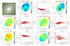 |
Fig. C.1 Luminosity- and mass-weighted maps and radial profiles for object 81461302615. Symbols are as in Fig. 3. |
All Tables
Median values of the covariance error ellipses for all the objects in the sample: position angle (θ), ellipticity (e), and Pearson’s coefficient (rxy).
Median light-weighted and mass-weighted gradients in linear and logarithmic space.
Comparison table providing the most relevant previous studies on stellar population gradients.
Stellar population gradients of the master radial profiles in linear and logarithmic space.
All Figures
|
Fig. 1 Properties of the analyzed sample from the ALHAMBRA catalog. a) Best photometric redshift distribution, b) stellar mass distribution, c) mass versus isophotal area relation, and d) color (mF365W−mF582W) versus stellar mass diagram. Gray symbols correspond to the total ALHAMBRA sample. Dashed histograms and open circles correspond to our initial sample, and blue histograms and symbols correspond to our final sample of 29 early-type galaxies after quality control cuts. The dashed black line represents the arbitrary red sequence-blue cloud division at mF365W−mF582W < 1.7. |
| In the text | |
|
Fig. 2 Color images of the 29 massive early-type galaxies analyzed in this paper. Each image corresponds to 22′′ × 22′′ centered on each target. The number of each image corresponds to the ID from Table A.1. |
| In the text | |
|
Fig. 3 Luminosity-weighted stellar population properties maps and radial profiles analyzed using E-MILES-based models for the example object 81461302615. Left column: 2D maps for log Age, [Fe/H], and Av covering an area of 22′′ × 22′′ around the target galaxy. The color range has been chosen to highlight inhomogeneities. Right column: log Age, [Fe/H], and Av as a function of the circularized galactocentric distance R′ (see Sect. 5). Each red circle corresponds to a bin in the 2D map. The black dashed line corresponds to the error-weighted linear fitting. Black crosses correspond to outliers identified during the sigma-clipping process and were not considered during the fit. |
| In the text | |
|
Fig. 4 Goodness-of-fit map, χ2, for the example object 81461302615. |
| In the text | |
|
Fig. 5 Integrated versus spatially resolved stellar masses derived from MUFFIT for the 29 massive early-type galaxies analyzed in this paper. Both BC03 and E-MILES SSP models were used. Symbols enclosed in squares indicate the six peculiar cases analyzed in Sect. 5.1. A normal distribution has been fit to the difference between the x-axis and the y-axis. The mean and standard deviation is labeled as Δ. The black dashed line shows the one-to-one relation. |
| In the text | |
|
Fig. 6 Integrated versus spatially resolved ages and metallicities derived from MUFFIT for the 29 massive early-type galaxies analyzed in this paper. Both BC03 and E-MILES SSP models were used. Symbols enclosed in squares indicate the six peculiar cases analyzed in Sect. 5.1. A normal distribution has been fit to the difference between the x-axis and the y-axis. The mean and standard dispersion is labeled as Δ in each panel. The black dashed line shows the one-to-one relation. |
| In the text | |
|
Fig. 7 Spatially resolved ages and metallicities versus mass. The lines indicate the relation obtained in Gallazzi et al. (2005), where the solid line corresponds to the median distribution and the dashed lines to the 16th and 84th percentiles. Symbols enclosed in squares indicate the six peculiar cases analyzed in Sect. 5.1. |
| In the text | |
|
Fig. 8 Difference stellar population values between our study and SDSS (Gallazzi et al. 2005) as a function of AgeL (top panel) and [Fe/H]L (bottom panel) from this study. Photometric values of our analysis were determined in the same aperture size as SDSS (3′′). The black dashed line shows the one-to-one relation. |
| In the text | |
|
Fig. 9 Stacked covariance error ellipses, at the 95% confidence level, of the stellar population parameters for all the objects in the sample. The red lines illustrate the minor and major axis of each ellipse, while the black lines correspond to the median values for the entire sample for E-MILES models. |
| In the text | |
|
Fig. 10 Histogram of the position angle (θ), ellipticity (e), and Pearson’s coefficient (rxy) for E-MILES models. The related variables are shown at the top of each column. |
| In the text | |
|
Fig. 11 Histograms of the linear space gradients for log AgeL (upper panel), [Fe/H]L (middle panel), and Av (bottom panel) for different SSP models. The median μ values are labeled in each panel. The six objects with peculiar profiles (Sect. 5.1) have been removed from the analysis. |
| In the text | |
|
Fig. 12 Distribution of age and metallicity gradients for early-type galaxies obtained in previous studies. All values have been taken from Table 3. The dashed lines represent the stellar population gradients obtained in this work. |
| In the text | |
|
Fig. 13 Stellar population gradients AgeL, [Fe/H]L , and Av, in logarithmic space as a function of stellar mass. BC03 and E-MILES, SSP models have been included. Open circles correspond to Illustris simulation measurements in the outer (1–2 Reff) galaxy region (Cook et al. 2016). Dashed black lines show flat gradients. The six objects with peculiar profiles (Sect. 5.1) have been removed from the analysis. |
| In the text | |
|
Fig. 14 Stacked radial profiles of log AgeL, [Fe/H]L, and Av. The left panels present the case of the E-MILES SSP models, and the right panels show the case of BC03. Gray open symbols correspond to the stellar population values of each individual bin in each spatially resolved object. Stars have been obtained by averaging the stellar population values of the sample in constant bins of 0.2 Reff between 0 ≤ R ≤ 3.6 Reff. The error bars are the standard deviation of the mean. When available, the profiles obtained by CALIFA (González Delgado et al. 2015) have been overplotted. MaNGA (Goddard et al. 2017) for early-type galaxies with log M⋆> 11.0 was also considered. The dashed black line corresponds to the best linear fit of the average stellar population values (stars). |
| In the text | |
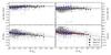 |
Fig. 15 Same as Fig. 14, but for the mass-weighted properties. |
| In the text | |
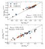 |
Fig. B.1 Same as Fig. 6, but for mass-weighted properties. |
| In the text | |
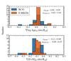 |
Fig. B.2 Same as Fig. 11, but for mass-weighted stellar properties. |
| In the text | |
 |
Fig. B.3 Same as Fig. 13, but for mass-weighted stellar properties. |
| In the text | |
|
Fig. C.1 Luminosity- and mass-weighted maps and radial profiles for object 81461302615. Symbols are as in Fig. 3. |
| In the text | |
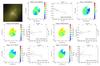 |
Fig. C.2 Same as Fig. C.1, but for object 81422100334. |
| In the text | |
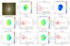 |
Fig. C.3 Same as Fig. C.1, but for object 81421207571. |
| In the text | |
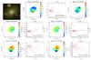 |
Fig. C.4 Same as Fig. C.1, but for object 81422303905. |
| In the text | |
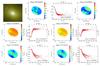 |
Fig. C.5 Same as Fig. C.1, but for object 81422406945. |
| In the text | |
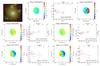 |
Fig. C.6 Same as Fig. C.1, but for object 81432100744. |
| In the text | |
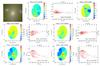 |
Fig. C.7 Same as Fig. C.1, but for object 81441106089. |
| In the text | |
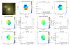 |
Fig. C.8 Same as Fig. C.1, but for object 81451305824. |
| In the text | |
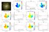 |
Fig. C.9 Same as Fig. C.1, but for object 81481104825. |
| In the text | |
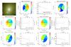 |
Fig. C.10 Same as Fig. C.1, but for object 81421106337. |
| In the text | |
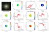 |
Fig. C.11 Same as Fig. C.1, but for object 81451206302. |
| In the text | |
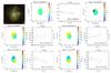 |
Fig. C.12 Same as Fig. C.1, but for object 81461400772. |
| In the text | |
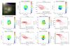 |
Fig. C.13 Same as Fig. C.1, but for object 81473405681. |
| In the text | |
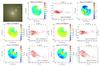 |
Fig. C.14 Same as Fig. C.1, but for object 81473406818. |
| In the text | |
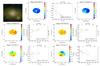 |
Fig. C.15 Same as Fig. C.1, but for object 81474201317. |
| In the text | |
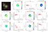 |
Fig. C.16 Same as Fig. C.1, but for object 81474307526. |
| In the text | |
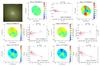 |
Fig. C.17 Same as Fig. C.1, but for object 81474404152. |
| In the text | |
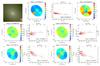 |
Fig. C.18 Same as Fig. C.1, but for object 81474404716. |
| In the text | |
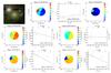 |
Fig. C.19 Same as Fig. C.1, but for object 81481201181. |
| In the text | |
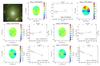 |
Fig. C.20 Same as Fig. C.1, but for object 81481402928. |
| In the text | |
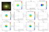 |
Fig. C.21 Same as Fig. C.1, but for object 81421103140. |
| In the text | |
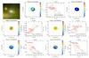 |
Fig. C.22 Same as Fig. C.1, but for object 81422407693. |
| In the text | |
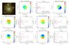 |
Fig. C.23 Same as Fig. C.1, but for object 81431100706. |
| In the text | |
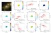 |
Fig. C.24 Same as Fig. C.1, but for object 81473103857. |
| In the text | |
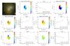 |
Fig. C.25 Same as Fig. C.1, but for object 81473111498. |
| In the text | |
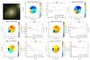 |
Fig. C.26 Same as Fig. C.1, but for object 81474103381. |
| In the text | |
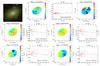 |
Fig. C.27 Same as Fig. C.1, but for object 81482205540. |
| In the text | |
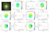 |
Fig. C.28 Same as Fig. C.1, but for object 81481401355. |
| In the text | |
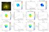 |
Fig. C.29 Same as Fig. 3 but for object 81422404933. |
| In the text | |
Current usage metrics show cumulative count of Article Views (full-text article views including HTML views, PDF and ePub downloads, according to the available data) and Abstracts Views on Vision4Press platform.
Data correspond to usage on the plateform after 2015. The current usage metrics is available 48-96 hours after online publication and is updated daily on week days.
Initial download of the metrics may take a while.