| Issue |
A&A
Volume 609, January 2018
|
|
|---|---|---|
| Article Number | A68 | |
| Number of page(s) | 19 | |
| Section | Astronomical instrumentation | |
| DOI | https://doi.org/10.1051/0004-6361/201630301 | |
| Published online | 09 January 2018 | |
Full-Stokes polarimetry with circularly polarized feeds
Sources with stable linear and circular polarization in the GHz regime⋆
1 Max-Planck-Institut für Radioastronomie, Auf dem Hügel 69, 53121 Bonn, Germany
e-mail: This email address is being protected from spambots. You need JavaScript enabled to view it.
2 Fraunhofer Institute for High Frequency Physics and Radar Techniques FHR, Fraunhoferstrasse 20, 53343 Wachtberg, Germany
3 IAPS-INAF, via Fosso del Cavaliere 100, 00133 Roma, Italy
4 Department of Astronomy, University of Michigan, 311 West Hall, 1085 S. University Avenue, Ann Arbor, MI 48109, USA
Received: 21 December 2016
Accepted: 30 May 2017
Abstract
We present an analysis pipeline that enables the recovery of reliable information for all four Stokes parameters with high accuracy. Its novelty relies on the effective treatment of the instrumental effects even before the computation of the Stokes parameters, contrary to conventionally used methods such as that based on the Müller matrix. For instance, instrumental linear polarization is corrected across the whole telescope beam and significant Stokes Q and U can be recovered even when the recorded signals are severely corrupted by instrumental effects. The accuracy we reach in terms of polarization degree is of the order of 0.1–0.2%. The polarization angles are determined with an accuracy of almost 1°. The presented methodology was applied to recover the linear and circular polarization of around 150 active galactic nuclei, which were monitored between July 2010 and April 2016 with the Effelsberg 100-m telescope at 4.85 GHz and 8.35 GHz with a median cadence of 1.2 months. The polarized emission of the Moon was used to calibrate the polarization angle measurements. Our analysis showed a small system-induced rotation of about 1° at both observing frequencies. Over the examined period, five sources have significant and stable linear polarization; three sources remain constantly linearly unpolarized; and a total of 11 sources have stable circular polarization degree mc, four of them with non-zero mc. We also identify eight sources that maintain a stable polarization angle. All this is provided to the community for future polarization observations reference. We finally show that our analysis method is conceptually different from those traditionally used and performs better than the Müller matrix method. Although it has been developed for a system equipped with circularly polarized feeds, it can easily be generalized to systems with linearly polarized feeds as well.
Key words: polarization / techniques: polarimetric / galaxies: active / radio continuum: galaxies / methods: data analysis / galaxies: jets
The data used to create Fig. C.1 are only available at the CDS via anonymous ftp to cdsarc.u-strasbg.fr (130.79.128.5) or via http://cdsarc.u-strasbg.fr/viz-bin/qcat?J/A+A/609/A68
© ESO, 2018
1. Introduction
As an intrinsic property of non-thermal emission mechanisms, the linear and circular polarization from astrophysical sources carry information about the physical conditions and processes in the radiating regions (e.g., Laing 1980; Wardle et al. 1998; Homan et al. 2009). Propagation through birefringent material – such as the intergalactic and interstellar medium – can further generate, modify, or even eliminate the polarized part of the transmitted radiation (e.g., Pacholczyk 1970; Jones & O’Dell 1977; Huang & Shcherbakov 2011). Consequently, processes that introduce variability in the emitting or transmitting regions induce dynamics in the observed polarization parameters (e.g., Marscher et al. 2008; Myserlis et al. 2014). Although these processes increase the complexity, they carry information about the mechanisms operating at the emitting regions.
The measured degree of linear and especially circular polarization of extragalactic sources in the radio window, is usually remarkably low. Klein et al. (2003) studied the B3-VLA sample in the range from 2 GHz to 10 GHz to find that the average linear polarization degree ranges from ~ 3.5% to 5%. Myserlis (2015) studied the circular polarization of almost 45 blazars in the GHz regime and found a population median of around 0.4%. Consequently, despite its importance, the reliable detection of polarized emission is particularly challenging especially when propagation and instrumental effects as well as variability processes are considered.
In the following, we present a pipeline for the reconstruction of the linear and circular polarization parameters of radio sources. The pipeline includes several correction steps to minimize the effect of instrumental polarization, allowing the detection of linear and circular polarization degrees as low as 0.3%. The instrumental linear polarization is calculated across the whole telescope beam and hence can be corrected for the observations of both point-like and extended sources. The methodology was developed for the 4.85 GHz and 8.35 GHz receivers of the 100-m Effelsberg telescope. Although these systems are equipped with circularly polarized feeds, our approach can easily be generalized for telescopes with linearly polarized feeds as well.
The consistency of our method is tested with a study of the most stable sources in our sample (in terms of both linear and circular polarization). Their stability indicates that physical conditions such as the ordering, magnitude, or orientation of their magnetic field remain unchanged over long timescales. The corresponding polarization parameters are reported for the calibration of polarization observations. We report both polarized and randomly polarized (unpolarized) sources. Conventionally, the latter are used for estimating the instrumental effects and the former to calibrate the data sets and quantify their variability.
The paper is structured as follows. In Sect. 2 an introduction to the technical aspects of the observations is presented. In Sect. 3 we present the methodology we developed to extract the polarization parameters with high accuracy. Our approach relies mainly on the careful treatment of the instrumental linear and circular polarization, discussed in Sects. 3.2 and 3.7, respectively, as well as the correction of instrumental rotation presented in Sect. 3.6. In Sect. 4 we perform a qualitative comparison between our method and the Müller matrix one. In Sect. 5 we describe the statistical analysis of the results obtained with our methodology and report on sources with stable linear and circular polarization. Finally, a discussion and the conclusions of our work are presented in Sect. 6.
Throughout the manuscript we use the conventions adopted by Commissions 25 and 40 at the 15th General Assembly of the IAU in 1973:
the reference frame of Stokes parameters Q and U is that of right ascension and declination with the polarization angle starting from north and increasing through east;
positive circular polarization measurements correspond to right-handed circular polarization.
This circular polarization convention is also in agreement with the Institute of Electrical and Electronics Engineers (IEEE) standard, according to which the electric field of a positive or right-handed circularly polarized electromagnetic wave rotates clockwise for an observer looking in the direction of propagation (IEEE Standards Board 1979).
2. Observations
The data set we discuss here was obtained with the Effelsberg 100-m telescope at 4.85 GHz and 8.35 GHz. The corresponding receivers are equipped with circularly polarized feeds (Table 1). A short description of the Stokes parameter measurement process using such systems is provided in Sect. 3.1.
The data set covers the period between July 2010 and April 2016. Until January 2015 the observations were conducted within the framework of the F-GAMMA monitoring program1 (Fuhrmann et al. 2016); beyond January 2015, data were obtained as part of multi-frequency monitoring campaigns on selected sources. The median cadence is around 1.2 months. The average duration of the observing sessions is 1.3 days.
Receiver characteristics.
The observations were conducted with “cross-scans”, that is, by slewing the telescope beam over the source position in two perpendicular directions. For the data set considered here those passes (hereafter termed “sub-scans”) were performed along the azimuth and elevation directions. The advantage of the cross-scan method is that it allows one to correct for the power loss caused by possible telescope pointing offsets. A detailed description of the observing technique is given by Angelakis et al. (2015).
In Sect. 3 we give a detailed description of the methodology followed for the reconstruction of the total flux density I, the degree of linear and circular polarization ml and mc, and the polarization angle, χ. The number of sources with at least one significant measurement (signal-to-noise ratio, S/N ≥ 3) of any of I, ml, χ or mc, is shown in Table 2, where we also list the mean uncertainty and cadence of the significant measurements at both frequencies.
Number of sources with at least one significant data point (S/N ≥ 3), mean uncertainty, and cadence of significant I, ml, mc, and χ measurements.
3. Full-Stokes polarimetry
In the current section we present the steps taken for reconstructing the circular and linear polarization parameters of the incident radiation from the observables delivered by the telescope. Our approach aims at recovering the polarization state outside the terrestrial atmosphere.
Our methodology is readily applicable to systems with circularly polarized feeds and can also easily be modified for systems with linearly polarized feeds. The latter are sensitive to the horizontal, Eh(t), and vertical, Ev(t), linearly polarized electric field components of the incident radiation. The Stokes parameters in terms of these components can be written as: 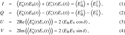 where EH,V are the amplitudes of the two orthogonal linearly polarized electric field components and δ is the phase difference between Eh(t) and Ev(t). A comparison between the Stokes parameterizations for linear (Eqs. (1)–(4)) and circular bases (Eqs. (7)–(10)) shows that for systems with linearly polarized feeds, the treatment of Stokes I needs to be kept constant, while Stokes Q, U and V should be treated as Stokes V, Q and U for systems with circularly polarized feeds, respectively. As an example, for systems with linearly polarized feeds, the instrumental polarization correction scheme presented in Sect. 3.2 should be applied in the U-V instead of the Q-U space, while the analysis of Sect. 3.7 should be applied to Stokes Q instead of V.
Figure 1 serves as a schematic summary of the analysis sequence. Each analysis level is labeled with an index (e.g., L1, L2, etc.) and is discussed in the section noted in that flow chart. The mean effect of each correction step is listed in Table 3.
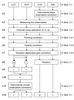 |
Fig. 1 Schematic summary of the analysis sequence. Each analysis level is labeled with an index on the left and is discussed in the section noted on the right. The mean effect of each correction step is listed in Table 3. |
Average percentage effect of each correction step on all Stokes parameters.
3.1. Measuring the Stokes parameters
Because our receivers are sensitive to the left- and right-hand circularly polarized components of the electric field, it is convenient to express the incident radiation in a circular basis: 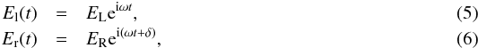 where EL,R are the amplitudes of the two (orthogonal) circularly polarized electric field components, ω is the angular frequency of the electromagnetic wave and δ is the phase difference between El(t) and Er(t).
The four Stokes parameters can then be written in terms of El(t) and Er(t) (omitting the impedance factors), as: 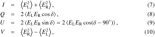 where ⟨⟩ denotes averaging over time to eliminate random temporal fluctuations of EL, ER and δ (e.g., Cohen 1958; Kraus 1966). A detailed discussion of the Stokes parametrization is given by Chandrasekhar (1950), Kraus (1966), Jackson (1998).
The system measures the four Stokes parameters by correlation operations, that is, multiplication and time averaging of the signals El(t) and Er(t), based on the parametrization of Eqs. (7)−(10): 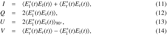 where the “*” denotes the complex conjugate and the subscript “90°” of Eq. (13) denotes that the correlation is performed after an additional phase difference of 90° is introduced between El(t) and Er(t). The auto-correlations of El(t) and Er(t) – needed for I (Eq. (11)) and V (Eq. (14)) – are processed separately in two receiver channels labeled LCP and RCP, respectively. On the other hand, the two cross-correlations of El(t) and Er(t) – needed for Q (Eq. (12)) and U (Eq. (13)) – are delivered in yet another pair of channels labeled COS and SIN. The LCP, RCP, COS and SIN channel data sets constitute the input for our pipeline (Fig. 1, level L1).
The alt-azimuthal mounting of the telescope introduces a rotation of the polarization vector in the Q-U plane by the parallactic angle, q (Fig. 1, level L8). In the general case, a potential gain difference between the COS and SIN channels introduces an additional rotation, φ. The angle φ vanishes once we balance the COS and SIN channel gains (Sect. 3.4; Fig. 1, level L4) but we need to take it into account when we calculate Stokes Q and U using the COS and SIN signals before the channel cross-calibration: ![Mathematical equation: \begin{equation} \label{eq:lp_domains} \left[ \begin{array}{c} Q\\U \end{array} \right] = \left[ \begin{array}{cr} \cos (2q + \phi) & -\sin (2q + \phi) \\ \sin (2q + \phi) & \cos (2q + \phi) \end{array} \right] \cdot \left[ \begin{array}{c} \mathrm{SIN}\\-\mathrm{COS} \end{array} \right] . \end{equation}](/articles/aa/full_html/2018/01/aa30301-16/aa30301-16-eq37.png) (15)Throughout the following analysis we occasionally express Q and U in either of the default north-east or the azimuth-elevation (azi-elv) reference frames. We differentiate the latter case by explicitly using the notation Qazi,elv or Uazi,elv, which can be calculated by setting q = 0 in Eq. (15).
(15)Throughout the following analysis we occasionally express Q and U in either of the default north-east or the azimuth-elevation (azi-elv) reference frames. We differentiate the latter case by explicitly using the notation Qazi,elv or Uazi,elv, which can be calculated by setting q = 0 in Eq. (15).
In Fig. 2 we show an example of an ~11% linearly polarized point-like source in LCP, RCP, COS and SIN channels. The Stokes I, Q, U and V are computed from Eqs. (7)–(10) and (15) once the source amplitude in those channels is known (Sect. 3.3; Fig. 1, level L12).
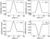 |
Fig. 2 Example of the same sub-scan in all channels on the source 3C 286 at 4.85 GHz. The abscissa is the offset from the commanded position of the source. The LCP and RCP channel data sets are shown in the upper row while the COS and SIN data sets are shown in the lower row. The target source is ~11% linearly polarized. |
3.1.1. Feed ellipticity and the measurement of Stokes parameters
Equations (5) to (15) describe the measurement of Stokes parameters for systems with ideal circularly polarized feeds. For such systems, the recorded left- and right-hand circularly polarized electric field components are perfectly orthogonal. In reality, instrumental imperfections lead to a (slight) ellipticity of the circular feed response. In this case, a small fraction of the incident left-hand circularly polarized electric field component is recorded by the right-hand circularly polarized channel of the system and vice versa.
The feed ellipticity can lead to deviations of the measured Stokes parameters from the incident ones. In Appendix A we provide an elementary approach to derive a rough estimate of the effect for the systems we used. A thorough study instead can be found in McKinnon (1992) or Cenacchi et al. (2009), for example. For Stokes I, we estimate that those deviations are at the level of 1 mJy for our data set, which is much less than the average uncertainty of our measurements (15–20 mJy, Table 2). Stokes Q and U on the other hand can be significantly modified by the feed ellipticity effect. A novel methodology to correct for the system-induced linear polarization across the whole telescope beam is described in Sect. 3.2. Finally, Stokes V is practically not affected in that simplified approach because the additional LCP and RCP terms introduced by the feed ellipticity (Eqs. (A.15) and (A.16)) cancel out. Nevertheless, as described in Sect. 3.7, our measurements suffer from instrumental circular polarization, which is most likely caused by a gain imbalance between the LCP and RCP channels. Two independent methodologies for the instrumental circular polarization correction are presented in Sect. 3.7.1.
3.2. Correcting for instrumental linear polarization
Instrumental imperfections manifest themselves as a cross-talk between the signals El(t) and Er(t). This can be best seen in unpolarized sources for which their cross-correlation is not null, contrary to what is theoretically expected (Eqs. (8) and (9)). Figure 3 shows an example of Qazi,elv and Uazi,elv data sets of a linearly unpolarized source. Instead of the expected constant, noise-like signal, spurious patterns are clearly visible. Their amplitudes can be up to ~ 0.5% of the total flux density (Fig. 4). Those signals can also be interpreted as “slices” of the polarized beam patterns over the azimuth and elevation directions.
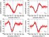 |
Fig. 3 Stokes Qazi,elv (left column) and Uazi,elv (right column) data sets recorded at 4.85 GHz for the unpolarized, point-like source NGC 7027 in the two scanning directions; the azimuth in the top row and the elevation in the bottom row. Instead of the expected flat, noise-like pattern, the presence of spurious signals is clearly visible in both scanning directions. The instrumental polarization, calculated by the instrument model M, is shown in each panel with a smooth black line. The dashed blue lines mark the source position along the scanning direction. |
To correct for the instrumental polarization (Fig. 1, level L2), we describe the telescope response to unpolarized sources with one instrument model M for each of the Qazi,elv and Uazi,elv along azimuth and elevation. Each M is written as a sum of j Gaussians or first derivatives of Gaussians selected empirically:  (16)where Fj is a Gaussian or first derivative of Gaussian with amplitude αjI, peak offset (μ−βj) and full width at half maximum (FWHM) γjσ. The explicit functional form of the models we used for the 4.85 GHz and 8.35 GHz receivers are given in Appendix B. The parameters I, μ, and σ in Eq. (16) are the average values between the LCP and RCP data set amplitudes, peak offsets, and FWHMs, respectively. The identification of the optimal instrument model for a given observing session from this family of models requires the evaluation of the parameters αj, βj, and γj.
For the evaluation of αj, βj, and γj we fit all observations on linearly unpolarized sources simultaneously. We first concatenate all sub-scans (index i in Eq. (17)) on all sources (index k). Subsequently, each of the four data sets is fitted with a function of the form: 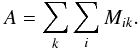 (17)In these terms, A is simply a concatenation of a total of i·k instrument models of the form M. In Fig. 4 we show the fitted instrument models for 65 observing sessions. The variability of the plotted models is comparable to the respective errors of the fit, which indicates that the instrumental polarization remained fairly stable throughout the examined period of 5.5 yr.
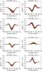 |
Fig. 4 Generated Stokes Q and U instrument models in the two scanning directions, the azimuth in the top panels and the elevation in the bottom panels for (a) the 4.85 GHz (upper two rows) and (b) 8.35 GHz (lower two rows) receivers. The models were generated for 65 observing sessions. The variability of the plotted models is comparable to the respective errors of the fit. |
After having optimized αj, βj, and γj for a given session, we remove the instrumental polarization from each sub-scan, in two steps:
We first substitute the measured I, μ, and σ in Eq. (16) to determine the explicit form of the instrumental polarization in that sub-scan.
We then subtract this instrumental effect from the observed Qazi,elv and Uazi,elv.
An example is shown in Fig. 5. With this approach, the scatter of the measured polarization parameters can be dramatically decreased owing to the fact that each sub-scan is treated separately (Fig. 6).
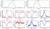 |
Fig. 5 Example of the instrumental linear polarization correction for an elevation sub-scan at 4.85 GHz. The observed COS/SIN (or equivalently Qelv/Uelv) signals are shown with red in the middle and bottom rows, immediately below the LCP signal, while the corrected signals are shown with blue immediately below the RCP signal. The correction is performed by subtracting the expected instrumental polarization signals (smooth black lines) from the observed Qelv and Uelv data sets (2nd and 3rd column of the middle and bottom rows). The instrumental polarization signals are calculated by substituting the measured mean amplitude I, peak offset μ, and FWHM σ of the LCP and RCP signals (top row) in the instrument model M created for the given observing session. |
3.3. Measuring the observables
Once Qazi,elv and Uazi,elv have been corrected for instrumental polarization, the process of measuring the Stokes parameters requires first the precise determination of the source amplitudes in the LCP, RCP, COS, and SIN channels (Fig. 1, level L3). As an example, given the low degree of circular polarization mc expected for our sources and because V is the difference between their amplitudes in LCP and RCP (Eq. (10)), an accuracy of at least 0.1% to 0.3% is required for an uncertainty of no more than about 0.1% to 0.2% in the mc. This precision would correspond to a 3–5σ significance for a 0.5% circularly polarized source.
Our tests showed that the most essential element for the amplitude measurement is accurate knowledge of the telescope response pattern and particularly the accurate determination of the baseline level. We found that the antenna pattern for a uniformly illuminated circular aperture, which is described by the Airy disk function: ![Mathematical equation: \begin{equation} \label{eq:airy_pattern} I = I_{0} \left[ \frac{2J_{1}(x)}{x} \right]^{2} , \end{equation}](/articles/aa/full_html/2018/01/aa30301-16/aa30301-16-eq64.png) (18)delivers significantly more accurate results than the commonly used Gaussian function, mainly because the latter fails to provide a precise description of the response beyond the FWHM. In Eq. (18), I0 is the maximum response level of the pattern at the center of the main lobe and J1 is the Bessel function of the first kind. In reality, the Effelsberg 100-m telescope beam is described by a more complex expression since its aperture is not uniformly illuminated, mainly due to the supporting structure of the secondary reflector. Nevertheless, the amplitude uncertainties using the Airy disk antenna pattern approximation (0.1−0.2%) are small enough to accommodate reliable low-circular-polarization-degree measurements. Figure 7 demonstrates the effectiveness of the Gaussian and the Airy disk beam pattern models in terms of the fractional residuals when we fit the observed data. Those are clearly minimized in the case of the Airy disk pattern.
(18)delivers significantly more accurate results than the commonly used Gaussian function, mainly because the latter fails to provide a precise description of the response beyond the FWHM. In Eq. (18), I0 is the maximum response level of the pattern at the center of the main lobe and J1 is the Bessel function of the first kind. In reality, the Effelsberg 100-m telescope beam is described by a more complex expression since its aperture is not uniformly illuminated, mainly due to the supporting structure of the secondary reflector. Nevertheless, the amplitude uncertainties using the Airy disk antenna pattern approximation (0.1−0.2%) are small enough to accommodate reliable low-circular-polarization-degree measurements. Figure 7 demonstrates the effectiveness of the Gaussian and the Airy disk beam pattern models in terms of the fractional residuals when we fit the observed data. Those are clearly minimized in the case of the Airy disk pattern.
 |
Fig. 6 Degree of linear polarization (top panel) and polarization angle (bottom panel) of the source 3C 48 at 4.85 GHz before (red circles) and after (blue triangles) applying the instrumental linear polarization correction. The data correspond to 23 sub-scans of the source within a single observing session. The dashed red and dotted blue lines indicate the 1σ regions around the mean values of the uncorrected and corrected data sets, respectively. The mean, μ, and standard deviation, σ, values of the corresponding data sets are shown in the legend. |
Ideally, the Airy disk could also be used for modeling the instrumental polarization (Eq. (16)) instead of Gaussians. This, however, would cause only an insignificant improvement (a small fraction of a percent) in the knowledge of the instrumental polarization magnitude. It would require a several-hundred-Jy source to cause a measurable effect.
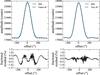 |
Fig. 7 Comparison between the Gaussian (left column) and Airy disk (right column) beam pattern models. The recorded data sets are shown in the top row with dark blue lines and the model fits with dashed, black lines. The corresponding fractional residuals, (data-model)/data, are given in the bottom row for a direct comparison between the models. |
3.4. Channel cross-calibration
Because of inevitable gain differences between the LCP, RCP, COS and SIN receiver channels, their response to the same photon influx is generally different (different number of “counts”). The level balancing – cross-calibration – of their signals is necessary before accurate polarization measurements can be conducted (Fig. 1, level L4).
The cross-calibration is performed by the periodical injection of a known polarization signal at the feed point of the receiver every 64 ms with a duration of 32 ms. For the used receivers this signal is generated by a noise diode designed to be: (a) circularly unpolarized; and (b) completely linearly polarized at a given polarization angle. The noise diode amplitude for each channel can be estimated as the average difference of the telescope response with the noise diode “on” and “off” in that channel. The channel cross-calibration is then achieved by expressing the LCP, RCP, COS and SIN amplitudes in noise diode units. The noise diode signal can be further calibrated to physical units, such as Jy, by comparison with reference sources (e.g., Ott et al. 1994; Baars et al. 1977; Zijlstra et al. 2008).
3.5. Post-measurement corrections
Before the final calculation of the Stokes parameters, the source amplitudes in channels LCP, RCP, COS and SIN are subjected to a list of post-measurement corrections which are discussed in detail in Angelakis (2007), Angelakis et al. (2009, 2015), Myserlis (2015).
3.5.1. Pointing correction
This step corrects for the power loss caused by offsets between the true source position and the cross-section of the two scanning directions (Fig. 1, level L5). Imperfect pointing may potentially also increase the scatter of the amplitudes from different sub-scans as, in the general case, the offset depends on the scanning direction. Assuming an Airy disk beam pattern, the amplitude corrected for a pointing offset poff, is 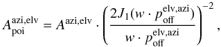 (19)where azi,elv denotes the scanning direction, Apoi is the source amplitude corrected for pointing offset, A is the uncorrected source amplitude, poff is the average absolute offset in arcsecs on the other scanning direction and w is calculated as
 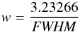 (20)where \begin{lxirformule}$\mathrm{FWHM}$\end{lxirformule} is the full width at half maximum of the telescope at the observing frequency in arcsecs. It is important to note that the offset in one direction (e.g., elevation) is used for correcting the amplitude in the other direction (e.g., azimuth).
The pointing correction is performed independently for each channel as the beam patterns are generally separated on the plane of the sky due to the miss-alignment between the feeds and the main axis of the telescope (“beam-squint” effect, e.g., Heiles 2002). In Fig. 8, we plot the density contours of all measured offsets from the source position separately for each channel. The beam-squint is directly evident as the miss-alignment of the contour peaks. For polarimetric observations, the beam-squint can introduce fake circular polarization, since the LCP and RCP beam patterns measure the source with different sensitivities.
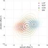 |
Fig. 8 Density plots of the measured offsets between the source position and the LCP, RCP, COS and SIN beam patterns for the 4.85 GHz receiver. The beam-squint can be clearly seen by the miss-alignment of the contour peaks (LCP: circle, RCP: upward-looking triangle, COS: square, SIN: downward-looking triangle). |
3.5.2. Opacity correction
The opacity correction corrects for the signal attenuation caused by the Earth’s atmosphere and relies on the calculation of the atmospheric opacity at the source position, τatm (Fig. 1, level L6).
Given the amplitude A of a measurement at an elevation ELV, the amplitude corrected for atmospheric opacity will be (21)where τatm is the atmospheric opacity at ELV. Under the assumption of a simple atmosphere model, τatm can be computed as a simple function of the zenith opacity τz
 (22)with AM being the airmass at ELV.
For any given observing session, a linear lower envelope is fitted to the airmass (AM)–system temperature (Tsys) scatter plot (Fig. 9) with Tsys taken from the off-source segment of all sub-scans. It can be shown that the inferred slope is a direct measure of the atmospheric opacity at zenith, τz (Angelakis 2007; Angelakis et al. 2009).
As we show in the example session of Fig. 9, τz is independent of LCP and RCP channels implying that the atmospheric absorption does not influence the polarization of the transmitted radiation. Hence, we applied the same τatm values to correct the amplitudes in all channels.
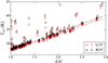 |
Fig. 9 LCP (red circles) and RCP (black triangles) system temperature (Tsys) measurements versus the airmass (AM) for one observing session at 4.85 GHz. The AM range is split into a given number of bins and the data points with the lowest Tsys within each bin (filled markers) are used to fit the two lower envelopes (solid lines). Their slopes are practically identical, indicating that the atmospheric absorption does not influence the polarization of the transmitted radiation. |
3.5.3. Elevation-dependent gain correction
The last correction accounts for the dependence of the telescope gain on elevation caused by the gravitational deformation of the telescope’s surface (Fig. 1, level L7).
The amplitude corrected for this effect given a value A measured at elevation ELV, will be  (23)where G(ELV) is the gain at elevation ELV. The gain is assumed to be a second order polynomial function of ELV. The parameters of the parabola used here have been taken from the Effelsberg website2.
Figure 10 shows the gain curve computed for one selected session. As can be seen there, the least-square-fit parabolas for the LCP and RCP data sets are very similar. Hence, the gravitational deformations do not affect the polarization measurements giving us the freedom to use the same correction factors G for all channels.
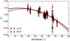 |
Fig. 10 Elevation-gain curves separately for LCP (red circles) and RCP (black triangles) data sets at 4.85 GHz. The similarity of the fitted parabolas indicates that the gravitational deformations do not affect the polarization measurements. |
As already stated, the correction factors used for the opacity and elevation-dependent gain corrections were identical for all channels. Consequently, they do not affect fractional expressions of the Stokes parameters such as the polarization degree or angle (Eqs. (40)–(42)), yet they are included formally in this step of the analysis as they affect the values of the total and polarized flux densities.
3.6. Correcting for instrumental rotation
Imprecise knowledge of the noise diode polarization angle potentially leads to poor knowledge of the power to be expected in the COS and SIN channels. Consequently, this leads to imperfect channel cross-calibration, which will manifest itself as an instrumental rotation. To study this effect we conducted observations of the Moon, which has a stable and well understood configuration of the polarization orientation.
The lunar black body radiation is linearly polarized. The polarization degree maximizes close to the limb while the polarization angle has an almost perfect radial configuration (e.g., Heiles & Drake 1963; Poppi et al. 2002; Perley & Butler 2013b).
We first performed the usual azimuth and elevation cross-scans centered on the Moon. Before estimating the polarization angle – which was the objective of this exercise – the observed Qazi,elv and Uazi,elv were corrected for instrumental polarization. As we discuss in Sect. 3.2 the instrument model for a sub-scan on a point source depends on the parameters measured in that sub-scan: I, μ and σ. For extended sources, the brightness distribution is needed instead. For this reason, for each sub-scan we first recovered the lunar brightness distribution by de-convolving the observed I with an Airy disk beam pattern. The de-convolution is then used to evaluate the explicit form of the instrumental polarization for that sub-scan by convolving the corresponding instrument model M with the calculated brightness distribution. Qazi,elv and Uazi,elv were then corrected for the instrumental polarization, which was calculated across the whole extent of the source.
We restricted the comparison of the observed and the expected polarization angle at the four points of the Moon’s limb that we probed. That is north, south, east and west. To quantify the instrumental rotation, we compared the median polarization angle around those four limb points with the values expected for the radial configuration. The east and west limb points are expected to be at 90° (or −90°), while the north and south limbs at 0° (or 180°). On the basis of 62 measurements at 4.85 GHz and 40 at 8.35 GHz, our analysis yields an average offset of 1.26° ± 0.11° for the former and −0.50° ± 0.12° for the latter. These are the values we consider to be the best guess for the instrumental rotation. All polarization angles reported in this paper have been corrected for this rotation.
There is evidence that the instrumental rotation depends on elevation. A Spearman’s test over all points on the Moon’s limb yielded a ρ of 0.69 (p = 0.01) and 0.79 (p = 0.02) for the 4.85 GHz and 8.35 GHz, respectively. Aside from this being a low-significance result it is also based on a narrow elevation range (~32.5°–50°). Yet, it is an indication that the instrumental rotation may have a more complex behavior.
3.7. Correcting for instrumental circular polarization
Imbalances between LCP and RCP channels similar to the ones discussed in Sect. 3.6 for COS and SIN can introduce instrumental circular polarization. Two effects with which the instrumental circular polarization is manifested are as follows:
As we show in Fig. 11, the distributions of the circular polarization degree, mc, measurements are centered around a non-zero value.
We measure systematically non-zero circular polarization from circularly unpolarized sources. An example is the case of the planetary nebula NGC 7027 (point-like at the two frequencies we consider), a free-free emitter expected to be circularly and linearly unpolarized, for which non-zero circular polarization is measured (Fig. 11).
The instrumental circular polarization may be as high as ~0.5% to 1% – comparable to the mean population values at those frequencies – and shows significant variability. The latter is indicated by the significantly correlated and concurrent variability we observe in mc light curves of different sources. For example, in Fig. 12, we plot the locally normalized discrete correlation function (DCF, Lehar et al. 1992; Edelson & Krolik 1988) between the mc light curves of two randomly chosen bright sources in our sample, namely 4C +38.41 and CTA 102, before and after the instrumental polarization correction. For the uncorrected data, the most prominent maxima appear at zero time lag where the correlation factor is 0.8 ± 0.2 and 0.7 ± 0.2 for the 4.85 GHz and 8.35 GHz data, respectively. These are also the only DCF maxima above the 3σ significance level.
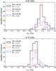 |
Fig. 11 Distributions of the circular polarization degree, mc, measurements at 4.85 GHz (top) and 8.35 GHz (bottom) for three observing sessions (solid black, dashed red and dotted blue lines). The non-zero average values, shown in the legend, indicate the presence of instrumental circular polarization. The mc measurements of the planetary nebula NGC 7027, in the corresponding sessions, are marked with arrows (in the bottom plot, two arrows overlap). |
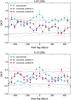 |
Fig. 12 Discrete correlation function (DCF) between the mc light curves of 4C +38.41 and CTA 102 before (cyan circles) and after the instrumental circular polarization correction using either method A (blue triangles) or method B (red squares) as described in the text. The corresponding 3σ significance levels are shown with dashed lines. |
3.7.1. Correction methods
If LD and RD are the diode signals in the LCP and RCP channels, respectively, the measured amplitudes of a source i in a session j expressed in diode units, will be:  where Lij and Rij are the source incident signals modulated only by the channel gain imbalance. The degree of circular polarization of the incident radiation can be recovered from the measured amplitudes
  and
and  by estimating the ratio r = RD/LD. Under the assumption that the noise diode is truly circularly unpolarized, r becomes unity. In reality, this is not the case and instrumental circular polarization emerges.
Using Eqs. (7), (10), (24) and (25), the corrected circular polarization degree can be written as: 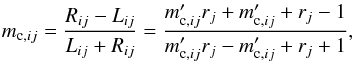 (26)where
  is the measured circular polarization degree estimated using and
  (27)Thus, in order to recover the corrected circular polarization degree mc,ij, we need to determine the ratio rj. In the following we show two independent methods to compute it (Fig. 1, level L11).
Method A: Zero-level of mc
The first method relies on the determination of the circular polarization degree that we would measure if the incident radiation was circularly unpolarized (zero level), that is, mc,ij = 0. We consider two estimates of the zero level:
the circular polarization degree of unpolarized sources (e.g.,NGC 7027); and
the average circular polarization degree of a sufficiently large, unbiased collection of sources.
We then compute rj by using either of these measurements as in Eq. (26) and setting mc,ij = 0. To avoid biases caused by small number statistics, we used the second estimate of the mc zero level above only for sessions where at least 20 sources were observed. To make sure that the average circular polarization degree is not affected by sources which are significantly polarized, we applied an iterative process to exclude them from the calculation similar to the gain transfer technique presented in Homan et al. (2001) and Homan & Lister (2006).
As shown in Fig. 13, the rj values calculated by either of the two mc zero-level estimates are in excellent agreement. Depending on the data availability, one or the other estimate was used. For the subset of sessions where both were available, the average rj was used.
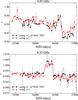 |
Fig. 13 Ratio r, calculated using both estimates of the circular polarization zero-level as described in method A for the 4.85 GHz (top) and 8.35 GHz (bottom) data sets. |
Method B: Singular value decomposition (SVD)
The second method requires the presence of a number of stable circular polarization sources within our sample, independently of whether they are polarized or not. If we divide Eqs. (24) and (25) we get  (28)For a source i with constant circular polarization, Qij does not depend on the session j, so that Qij = Qi. Consequently, any variability seen in the measured
  for these sources can only be induced by the system through rj. For the sources of constant circular polarization it can be written
  (29)or in matrix-vector form
  (30)Using the singular value decomposition method (SVD, e.g., Golub & Van Loan 2013), we can express matrix Q′ as a sum of matrices each of which has rank one. For i = 1,...,n sources with stable circular polarization observed over j = 1,...,m sessions and n ≤ m, this will be
 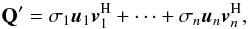 (31)where σi are the singular values of the matrix Q′ in decreasing magnitude and ui and vi are its left- and right-singular vectors, respectively. ui is of length n and vi of length m. If σ1/σ2 ≫ 1, Q′ can be approximated by the first term in Eq. (31) and one can write,
 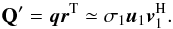 (32)This implies that the unknown vectors q and r are parallel to u1 and v1, respectively:
  with ab = σ1. In order to solve for a and b, we need at least one source of known circular polarization included in the list of n stable sources. Assuming that this is the first source of the set (i = 1), Q1 can be calculated from
 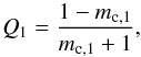 (35)where mc,1 is its known circular polarization degree, and using Eq. (29) we can write
 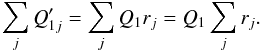 (36)Additionally, from Eq. (34), we have
 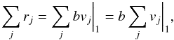 (37)where ∑ jvj | 1 is the sum of all the elements of vector v1. Therefore, using Eqs. (36) and (37), the factor b can be computed as:
 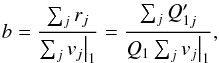 (38)and the factor a = σ1/b. Once b has been computed, Eq. (34) will give us vector r, the elements of which are the circular polarization correction factors rj to be used in Eq. (26).
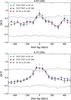 |
Fig. 14 Discrete correlation function (DCF) between the |
The SVD methodology was implemented using three sources: NGC 7027, 3C 48, and 3C 286. This subset of sources was selected as the best candidates with stable circular polarization based on the following criteria:
Stability of the observed circular polarization (even beingunpolarized). Assuming that the observed variability is asuperposition of the instrumental and the intrinsic polarizationvariability, the sources with the lowest  variability are the best candidates to be intrinsically stable.
Most frequently observed. This criterion ensures that we can apply method B to as many sessions as possible and account for the instrumental polarization that can show pronounced variability even on short timescales (Fig. 13).
For the analyzed data sets, the sources 3C 286 and 3C 48 best fulfill both of the above criteria. NGC 7027 was selected as the source assumed to have known circular polarization. Its free-free emission is expected to be circularly unpolarized (mc = 0) and hence its Q = 1 according to Eq. (35). For a session with no NGC 7027 data, we adopted a mock source of zero circular polarization to which we assigned as observed value the averaged over all sources in that session. A minimum of 20 sources was required in those cases. The circular polarization degree values for the other sources assumed stable (3C 286 and 3C 48 in our case) are not required for method B, which is one of the main advantages of this calibration technique.
The circular polarization stability of the selected sources is also advocated by:
The fact that they display the most significantly correlated andconcurrent variability in circular polarization(Fig. 14). Their low intrinsic circular polarizationvariability is supported by the coincidence of all lines there, aswell as by the fact that, for them, the zero time lag correlationexceeds the 5σ threshold.
The σ1/σ2 ratios for the 4.85 GHz and 8.35 GHz data using these sources were ~ 521 and ~ 540 (~ 27dB), respectively, justifying the approximation of with a single rank-one matrix.
3.7.2. Comparison between methods A and B, and the UMRAO database
In Fig. 12 we show the DCF of corrected circular polarization data for 4C +38.41 and CTA 102. The data corrected with methods A and B are shown separately. The improvement is directly evident in the radical decrease of the correlation factors at zero time lag. In fact, the zero time lag correlation does not exceed the 1σ level.
Figure 15 now shows the mc measurements of NGC 7027 before and after the correction for instrumental circular polarization with methods A and B. For the uncorrected data sets, we systematically measure non-zero mc with standard deviations of 0.4% and 0.2% at 4.85 GHz and 8.35 GHz, respectively. The corrected mc on the other hand, using methods A and B are in excellent agreement, appear very close to zero, and have standard deviations that are reduced to 0.1%.
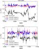 |
Fig. 15 mc measurements of NGC 7027 at 4.85 GHz (top) and 8.35 GHz (bottom) before (black circles) and after the instrumental circular polarization correction using both methods A (red triangles) and B (blue squares). |
For the sources with the most stable behavior, Table 9 lists their circular polarization measurements. Methods A and B agree well within the errors. Method B gives on average 0.016% smaller standard deviations than method A. This is most likely caused because method B assumes more sources with constant polarization than method A.
Finally, we compared the corrected circular polarization measurements using methods A and B with measurements from the UMRAO monitoring program (Aller & Aller 2013; Aller et al. 2016). The comparison was performed for five sources with overlapping data sets from both monitoring programs (~2010.5–2012.3), namely 3C 84, OJ 287, 3C 279, BL Lac and 3C 454.3. Specifically, we compared all concurrent data points within a maximum separation of 2 weeks. There are 110 and 59 such data points of the UMRAO data set overlapping with the results of methods A and B, respectively. In both cases we found a median absolute difference in the circular polarization degree measurements of only 0.2%. The corresponding data sets for the time range embracing the overlapping period are shown in Fig. C.1. The comparison of such contemporaneous measurements is particularly important because it can be used to detect or put strict limits on the very rapid variations usually observed in the circular polarization of active galactic nuclei (AGN) jets (Aller et al. 2003).
4. Comparison with the Müller matrix method
Traditionally the Müller matrix method has been the one adopted for treating the instrumental polarization. Here we carry out a comparison with our method.
The Müller matrix method is based on estimating the elements of the Müller matrix, M, which is a transfer function between the incident Sreal and the measured Sobs Stokes 4-vectors:  (39)A set of four independent measurements of sources with known Sreal are enough to solve the system of Eq. (39) and compute the M matrix elements. In case more measurements are available a fit can determine the best-guess values. The inverse M matrix is then applied to Sobs to correct for instrumental effects.
As discussed in Sect. 3.2, our methodology models and corrects for the instrumental linear polarization across the whole beam before extracting the Stokes Q and U data, while the Müller method has no handle on this. This can be essential for cases of low Q or U amplitudes which can be corrupted to the point that the telescope response pattern cannot be seen in the data. For the majority of such cases our methodology was able to recover the telescope response pattern (e.g., Qelv in Fig. 5). In milder cases our methodology resulted in peak offsets closer to the source position and FWHM values closer to the actual ones.
Another advantage of our approach is the milder conditions it requires. As discussed in Sect. 3.7.1, method A simply requires the observation of a circularly unpolarized source, and method B requires n sources with constant circular polarization with the need to know the exact value of mc only for one of them. The Müller method on the other hand, requires a good coverage of the Stokes parameter space and particularly for V.
To perform a quantitative comparison of the two techniques, we focused on the linear polarization results. First, we calculated I, Q, and U for all sources and observing sessions using both our methodology and the Müller method, accounting for all post-measurement corrections described in Sect. 3.5. For each session, the 3 × 3 Müller matrix was determined using all observations on the polarization calibrators shown in Table 4.
Polarization calibrators used for the Müller matrix method.
As a figure of merit for the comparison, we used the intra-session variability of I, Q, and U in terms of their standard deviation σI,Q,U. Since our sources are not expected to vary within a session (not longer than 3 days), any variability in I, Q, and U can naturally be attributed to instrumental effects. Consequently, the technique leading to lower variability must be providing a better handling of the instrumental effects. In our study we included measurements with linearly polarized flux of at least 15 mJy.
We performed two-sample Kolmogorov-Smirnov (KS) tests to compare the corresponding σI,Q,U distributions between the two techniques for three polarized flux ranges; all, high polarization (≥100 mJy), and low polarization (15–100 mJy). The results for the 4.85 GHz receiver are presented in Table 5 along with the median σI,Q,U values for either of the two techniques. The cases where the KS test rejects the null hypothesis that the two distributions are the same at a level greater than 5σ are marked with an asterisk.
For Stokes I, both methods perform equally well since the corresponding KS-test results show no significant difference between the σI distributions of the Müller method and our methodology. That is also the case for Stokes Q and U of the high polarization data.
Our approach performs significantly better for Stokes Q and U when we consider either the complete data set (all) or the low polarization data. The corresponding KS-test results show that the σQ,U distributions of the Müller method and our methodology are significantly different above the level of 5σ. A direct comparison of the median σQ,U values shows that our method delivers ~ 8% and ~ 28% more stable results for the complete data set (all) and the low polarization data, respectively. The main reason for this improvement is the instrumental linear polarization correction scheme of our methodology that treats each sub-scan separately, accounting for the instrumental polarization contribution across the whole beam (Sect. 3.2).
KS-test results (KS statistic D, and p-value) for the comparison between the σI,Q,U distributions for the 4.85 GHz data calibrated by the Müller method and our methodology.
5. Sources with stable polarization
The methodology described in Sect. 3 was used to compute the linear and circular polarization parameters of the observed sources at 4.85 GHz and 8.35 GHz. Once all four Stokes parameters have been computed, the degree of linear and circular polarization, ml and mc and the polarization angle χ, were calculated as: 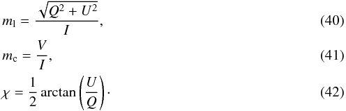 The corresponding errors were computed as the Gaussian error propagation of the uncertainties in the LCP, RCP, COS, and SIN amplitudes through Eqs. (7)–(10), (15) and (40)–(42). Finally, for each observing session, we computed the weighted average and standard deviation of the polarization parameters for all sub-scans on a given source, using their errors as weights.
Our data set includes a total of 155 sources and was examined to look for cases of stable linear and circular polarization characteristics to be listed as reference sources for future polarization observations. Because we are interested in identifying only cases with stable polarization parameters, we restricted our search to a sub-sample of 64 sources that were observed:
for at least three years; and
with a cadence of one measurement every 1 to 3 months.
In Fig. 16 we show the distributions of standard deviations σml, σmc, and σχ at 4.85 GHz and 8.35 GHz. The sources exhibit a broad range of variability in all polarization parameters. The threshold for our search was set to the 20th percentile, P20, that is, one fifth of the corresponding standard deviation distribution, marked by the dotted lines in those plots.
Sources with stable linear polarization degree, ml.
 |
Fig. 16 Standard deviation distributions of the linear polarization degree, σml, polarization angle, σχ, and circular polarization degree, σmc, measurements at 4.85 GHz (top row) and 8.35 GHz (lower row). The 20th percentile, P20, of each standard deviation distribution is marked by a dotted line. The circular polarization data contain the measurements corrected with both methods A (solid black line) and B (dashed red line) as described in Sect. 3.7.1. |
Sources with stable polarization angle, χ.
In Tables 6 and 7, we list the sources with the most stable ml and χ values at 4.85 GHz and 8.35 GHz. The names of sources for which both ml and χ were found to be stable at at least one observing frequency are marked in bold face. The reported sources exhibited significant linear polarization at least 95% of the times they were observed. Significant linear polarization measurements are considered as being those with a weighted mean of ml at least three times larger than the weighted standard deviation in the corresponding session. In Table 8 we list linearly unpolarized sources, that is, sources with no significant linear polarization measurements. For the latter, we report the average values of their ml 3σ upper limits.
Linearly unpolarized sources.
Finally, in Table 9, we list the sources with the most stable mc. For comparison, we list the average and standard deviation values of mc, corrected with both methods A and B as described in Sect. 3.7.1. Most of the sources in Table 9 exhibit mean mc values very close to zero and therefore are considered circularly unpolarized. However, 3C 286, 3C 295, 3C 48 and CTA 102 show significant circular polarization (⟨mc⟩ /σmc ≥ 3) at 4.85 GHz with at least one of the two correction methods.
Komesaroff et al. (1984) observed two of the sources presented in Table 9 between December 1976 and March 1982, namely CTA 102 and PKS 1127-14. At that time CTA 102 showed variable circular polarization degree, which suggests that its mc cannot be considered stable over such long time scales. On the other hand, PKS 1127-14 was found stable in mc, with a synchronous decrease in both Stokes I and V. The average circular polarization degree of PKS 1127-14 over that period was mc ≈ −0.1 ± 0.03%, which is very close to the value listed in Table 9. This finding places additional bounds on its mc stability, suggesting that it may have remained unchanged for ~40 yr.
Sources with stable circular polarization degree, mc.
The sources reported in Tables 6–9 show stable behavior in different polarization properties. Nevertheless there is a small subgroup, namely 3C 286, 3C 295, 3C 48 and NGC 7027, which remain stable in both linear and circular polarization throughout the period examined (2010.5–2016.3). Perley & Butler (2013a) and Zijlstra et al. (2008) show that these sources exhibit stable or well-predicted behavior also in Stokes I, and are therefore well suited for the simultaneous calibration of all Stokes parameters.
Previous studies have revealed a general tendency of the circular polarization handedness to remain stable over many years (e.g., Komesaroff et al. 1984; Homan & Wardle 1999; Homan et al. 2001). The consistency of the circular polarization sign may indicate either a consistent underlying ordered jet magnetic field component (e.g., toroidal or helical) or a general property of AGN with the sign of circular polarization set by the super-massive black hole (SMBH)/accretion disk system (e.g., Enßlin 2003).
We compared our data set with the one presented several decades ago in Komesaroff et al. (1984) to investigate the long-term stability of the circular polarization handedness, independently of the stability in the amplitude of mc. There are ten sources common to the two samples. Three of them – namely PKS 1127-14, 3C 273, and 3C 279 – show stable circular polarization handedness in both data sets with the same sign of mc. 3C 161 shows stable circular polarization handedness in both data sets but with the sign of mc reversed. The rest of the common sources – namely PKS 0235+164, OJ 287, PKS 1510-089, PKS 1730-130, CTA 102 and 3C 454.3 – show short-term variability of the circular polarization handedness in at least one of the two data sets. A thorough presentation of our circular polarization data set and its comparison with previous works will be presented in a future publication.
6. Discussion and conclusions
We present the analysis of the radio linear and circular polarization of more than 150 sources observed with the Effelsberg 100-m telescope at 4.85 GHz and 8.35 GHz. The observations cover the period from July 2010 to April 2016 with a median cadence of around 1.2 months. We developed a new methodology for recovering all four Stokes parameters from the Effelsberg telescope observables. Although our method has been implemented for an observing system with circularly polarized feeds, it is easily generalizable to systems with linearly polarized feeds.
The novelty of our approach relies chiefly on the thorough treatment of the instrumental effects. In fact, our method aims at correcting the observables already prior to the computation of the Stokes parameters. In contrast, conventional methodologies – like the Müller matrix – operate on the Stokes vector. Consequently, cases of instrumentally corrupted observables that would be conventionally unusable, can be recovered by the careful treatment of their raw data. Additionally, for the correction of the circular polarization, the Müller matrix method requires a good coverage of the parameter space. Our method on the other hand requires at most a small number of stable reference sources with the explicit knowledge of mc only for one of them. Finally, the Müller matrix method lacks the capacity to treat the shortest observation cycle (sub-scan) operating on mean values.
In our method, the instrumental linear polarization – which is most likely caused by the slight ellipticity of the circular feed response – is modeled across the whole beam on the basis of the telescope response to unpolarized sources. Each sub-scan is then cleaned of the instrumental contribution, separately. Our results indicate that the instrumental linear polarization of the systems we used remained fairly stable throughout the examined period of 5.5 yr.
For the treatment of the instrumental circular polarization we introduced two independent methods: the zero-leveling of the mc and the powerful singular value decomposition (SVD) method. Both rely on very few easy-to-satisfy requirements and give very similar results. The results of both methods are also in agreement with the UMRAO data set.
The clean data are then subjected to a series of operations including the opacity and elevation-gain corrections, which we found to be immune to the incident radiation’s polarization state. Moreover, the Airy disk beam pattern delivers amplitude estimates precise enough to accommodate reliable low-circular-polarization measurements.
All in all, our methodology allows us to minimize the uncertainties in linear and circular polarization degree at the level of 0.1–0.2%. The polarization angle can be measured with an accuracy of the order of 1°.
We have estimated the instrumental rotation potentially caused by our apparatus by observing the Moon, which has a simple radial configuration of the polarization angle, thereby providing an excellent reference for (a) estimating the instrumental rotation and (b) conducting absolute angle calibration. We found that the instrument introduces a minute rotation of 1.26° and −0.5° for 4.85 GHz and 8.35 GHz, respectively. What is however worth noting is that we found evidence that there must be an, at least, mild dependence of the rotation on the source elevation. For completeness further investigation is merited, despite the marginal magnitude of the effect.
Despite the conceptual differences between our method and that using the Müller matrix, we conducted a quantitative comparison of their effectiveness. We examined the intra-session variability in the linear polarization parameters. Those should remain unchanged over such short time scales even for intrinsically variable sources. Our methodology performs significantly better, particularly for low linear polarization observations (15–100 mJy polarized flux), where it delivers 28% more stable Stokes Q and U results than the Müller method.
After having reconstructed as accurately as possible the polarization state of our sample, we searched for sources with stable polarization characteristics. We found five sources with significant and stable linear polarization. A list of three sources remain constantly unpolarized over the entire period examined of almost 5.5 yr. A total of 11 sources were found to have stable circular polarization degree, four of which with non-zero mc. One of the sources with stable circular polarization degree, namely PKS 1127-14, was found to be stable and at the same level several decades ago by Komesaroff et al. (1984), suggesting that its mc may have remained unchanged for ~40 yr. Additionally, we found eight sources that maintain a stable polarization angle over the examined period. All this is provided to the community for future polarization observation reference.
Finally, we investigated the long-term stability of the circular polarization handedness for the ten sources common to both our sample and the data set presented in Komesaroff et al. (1984). Three sources show stable circular polarization handedness in both data sets with the same sign of mc, and one with the opposite sign, and the other six sources show short term variability of the circular polarization handedness in at least one of the two data sets.
Acknowledgments
This research is based on observations with the 100-m telescope of the MPIfR (Max-Planck-Institut für Radioastronomie) at Effelsberg. I.M. and V.K. were funded by the International Max Planck Research School (IMPRS) for Astronomy and Astrophysics at the Universities of Bonn and Cologne. This research has made use of data from the University of Michigan Radio Astronomy Observatory which has been supported by the University of Michigan and by a series of grants from the National Science Foundation, most recently AST-0607523. The authors thank A. Roy, the internal MPIfR referee, for his useful comments.
References
- Aller, H. D., & Aller, M. F. 2013, in The Innermost Regions of Relativistic Jets and Their Magnetic Fields, Granada, Spain [Google Scholar]
- Aller, H. D., Aller, M. F., & Plotkin, R. M. 2003, Astrophys. Space Sci., 288, 17 [Google Scholar]
- Aller, M. F., Aller, H. D., Hughes, P. A., & Latimer, G. E. 2016, in HAP Workshop: Monitoring the Non-Thermal Universe, Cochem, Germany [Google Scholar]
- Angelakis, E. 2007, Ph.D. Thesis, Max-Planck-Institut für Radioastronomie, http://hss.ulb.uni-bonn.de/2007/0968/0968.htm [Google Scholar]
- Angelakis, E., Kraus, A., Readhead, A. C. S., et al. 2009, A&A, 501, 801 [NASA ADS] [CrossRef] [EDP Sciences] [Google Scholar]
- Angelakis, E., Fuhrmann, L., Marchili, N., et al. 2015, A&A, 575, A55 [NASA ADS] [CrossRef] [EDP Sciences] [Google Scholar]
- Baars, J. W. M., Genzel, R., Pauliny-Toth, I. I. K., & Witzel, A. 1977, A&A, 61, 99 [NASA ADS] [Google Scholar]
- Cenacchi, E., Kraus, A., Orfei, A., & Mack, K.-H. 2009, A&A, 498, 591 [NASA ADS] [CrossRef] [EDP Sciences] [Google Scholar]
- Chandrasekhar, S. 1950, Radiative Transfer (Oxford: Clarendon Press) [Google Scholar]
- Cohen, M. H. 1958, Proc. IRE, 46, 172 [CrossRef] [Google Scholar]
- Edelson, R. A., & Krolik, J. H. 1988, ApJ, 333, 646 [NASA ADS] [CrossRef] [Google Scholar]
- Enßlin, T. A. 2003, A&A, 401, 499 [NASA ADS] [CrossRef] [EDP Sciences] [Google Scholar]
- Fuhrmann, L., Angelakis, E., Zensus, J. A., et al. 2016, A&A, 596, A45 [NASA ADS] [CrossRef] [EDP Sciences] [Google Scholar]
- Golub, G. H., & Van Loan, C. F. 2013, Matrix Computations, 4th edn. (JHU Press) [Google Scholar]
- Heiles, C. 2002, in Single-Dish Radio Astronomy: Techniques and Applications, 278, 131 [Google Scholar]
- Heiles, C. E., & Drake, F. D. 1963, Icarus, 2, 281 [NASA ADS] [CrossRef] [Google Scholar]
- Homan, D. C., & Lister, M. L. 2006, AJ, 131, 1262 [NASA ADS] [CrossRef] [Google Scholar]
- Homan, D. C., & Wardle, J. F. C. 1999, AJ, 118, 1942 [NASA ADS] [CrossRef] [Google Scholar]
- Homan, D. C., Attridge, J. M., & Wardle, J. F. C. 2001, ApJ, 556, 113 [NASA ADS] [CrossRef] [Google Scholar]
- Homan, D. C., Lister, M. L., Aller, H. D., Aller, M. F., & Wardle, J. F. C. 2009, ApJ, 696, 21 [NASA ADS] [Google Scholar]
- Huang, L., & Shcherbakov, R. V. 2011, MNRAS, 416, 2574 [NASA ADS] [CrossRef] [Google Scholar]
- IEEE Standards Board. 1979, ANSI/IEEE Std 149-1979, 61 [Google Scholar]
- Jackson, J. D. 1998, Classical Electrodynamics, 3rd edn. (Wiley-VCH), 832 [Google Scholar]
- Jones, T., & O’Dell, S. 1977, ApJ, 214, 522 [NASA ADS] [CrossRef] [Google Scholar]
- Klein, U., Mack, K.-H., Gregorini, L., & Vigotti, M. 2003, A&A, 406, 579 [NASA ADS] [CrossRef] [EDP Sciences] [Google Scholar]
- Komesaroff, M. M., Roberts, J. A., Milne, D. K., Rayner, P. T., & Cooke, D. J. 1984, MNRAS, 208, 409 [NASA ADS] [CrossRef] [Google Scholar]
- Kraus, J. D. 1966, Radio Astronomy (Cygnus-Quasar Books) [Google Scholar]
- Laing, R. A. 1980, MNRAS, 193, 439 [NASA ADS] [Google Scholar]
- Lehar, J., Hewitt, J. N., Burke, B. F., & Roberts, D. H. 1992, ApJ, 384, 453 [NASA ADS] [CrossRef] [Google Scholar]
- Marscher, A. P., Jorstad, S. G., D’Arcangelo, F. D., et al. 2008, Nature, 452, 966 [NASA ADS] [CrossRef] [PubMed] [Google Scholar]
- McKinnon, M. M. 1992, A&A, 260, 533 [NASA ADS] [Google Scholar]
- Myserlis, I. 2015, Ph.D. Thesis, Max-Planck-Institut für Radioastronomie, http://kups.ub.uni-koeln.de/6967/ [Google Scholar]
- Myserlis, I., Angelakis, E., Fuhrmann, L., et al. 2014, ArXiv eprints [arXiv:1401.2072] [Google Scholar]
- Ott, M., Witzel, A., Quirrenbach, A., et al. 1994, A&A, 284, 331 [NASA ADS] [Google Scholar]
- Pacholczyk, A. G. 1970, Radio astrophysics. Nonthermal processes in galactic and extragalactic sources, Series of Books in Astronomy and Astrophysics (San Francisco: Freeman) [Google Scholar]
- Perley, R. A., & Butler, B. J. 2013a, ApJS, 204, 19 [NASA ADS] [CrossRef] [Google Scholar]
- Perley, R. A., & Butler, B. J. 2013b, ApJS, 206, 16 [Google Scholar]
- Poppi, S., Carretti, E., Cortiglioni, S., Krotikov, V. D., & Vinyajkin, E. N. 2002, in Astrophysical Polarized Backgrounds, eds. S. Cecchini, S. Cortiglioni, R. Sault, & C. Sbarra, AIP Conf. Ser., 609, 187 [Google Scholar]
- Wardle, J., Homan, D., Ojha, R., & Roberts, D. 1998, Nature, 395, 457 [NASA ADS] [CrossRef] [Google Scholar]
- Zijlstra, A. A., van Hoof, P. A. M., & Perley, R. A. 2008, ApJ, 681, 1296 [NASA ADS] [CrossRef] [Google Scholar]
Appendix A: Feed ellipticity and the measurement of Stokes parameters
In this appendix we estimate the effect of feed ellipticity on the measurement of Stokes parameters. In the following, we provide an elementary approach where several aspects have been oversimplified, for example, parameters a and b in Eqs. (A.1) and (A.2) are considered real instead of complex numbers. This approach was selected in order to derive a rough estimate of the effect on the measured parameters. A thorough study of the effect can be found in McKinnon (1992) or Cenacchi et al. (2009), for example.
The feed ellipticity can be parameterized as a cross-talk between the left- and right-hand circularly polarized electric field components recorded by the system: 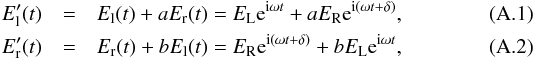 where EL,R are the amplitudes of the two incident (orthogonal) circularly polarized electric field components, ω is the angular frequency of the electromagnetic wave, δ is the phase difference between El(t) and Er(t) and a, b are the percentage of the incident left-hand polarized electric field component recorded by the right-hand polarized channel and vice versa. The primed and unprimed quantities in Eqs. (A.1) and (A.2) refer to the recorded and incident signals, respectively. The terms that contain parameters a and b appear due to the ellipticity of the circular feed response (see Eqs. (5) and (6) for comparison).
Using Eqs. (A.1) and (A.2), the LCP, RCP, COS and SIN signals can be written as:  where the “*” denotes the complex conjugate and the subscript “90°” of Eq. (A.6) denotes that an additional phase difference of 90° is introduced between
  and
and  . The real part of Eqs. (A.3)–(A.6), which is recorded by the system, is:
  To derive a rough estimate of the effect on the measurement of the four Stokes parameters, we can further simplify the above expressions by assuming that a ≈ b = k:
  The last terms in Eqs. (A.13) and (A.14) describe a contribution of Stokes I
 to the measured linearly polarized flux density as recorded by the COS and SIN channels. We can estimate the parameter k from the observations of linearly unpolarized sources. Such sources have a random phase difference δ, which means that ⟨cosδ⟩ = 0 and hence the first terms of Eqs. (A.13) and (A.14) are vanished. The last terms, on the other hand, describe the spurious instrumental linear polarization signals that we correct for using the instrument model (see Sect. 3.2). Thus the parameter k is described (across the whole beam) by the instrument model (e.g., Fig. 4) which is at maximum 0.005 for the systems we used. Therefore – in this simplified approach – we can exclude the second-order terms of k from Eqs. (A.11)–(A.14) since k2 → 0 (it is at maximum 2.5 × 10⁻⁵) which results in:
  Equations (A.15)–(A.18) can be used to estimate the effect of the feed ellipticity on the measurement of the Stokes parameters. The last terms in Eqs. (A.17) and (A.18) are removed by the instrumental linear polarization correction scheme as described in Sect. 3.2. Therefore, Stokes Q and U should not be affected by the feed ellipticity after this correction step. Stokes V remains also unaffected because the subtraction of LCP from RCP removes the last terms of Eqs. (A.15) and (A.16) which appear due to the feed ellipticity effect.
Finally, Stokes I seems to be affected by the feed ellipticity effect even in this elementary approach. The recorded Stokes I can deviate from the incident signal by 4kELERcosδ, which is proportional to the linear polarization of the source ( ). Using the average linearly polarized flux density over all our measurements (0.125 Jy) as an estimate of Stokes Q in the above expression we get:
  (A.19)Therefore, the measured Stokes I deviates from the incident signal by ~1 mJy on average. This value is much smaller than the average uncertainty of our measurements (15–20 mJy, Table 2). In fact, if we use the largest linearly polarized flux density that we have ever measured (2.116 Jy) we calculate that the feed ellipticity effect on Stokes I is at maximum 21 mJy, which is comparable to the average uncertainty.
The above discussion shows that, in most cases, the feed ellipticity does not seem to have any measurable effect on the Stokes parameter measurements once we account for the instrumental linear polarization (e.g., using the correction scheme presented in Sect. 3.2). The parameter which is mostly affected is Stokes I but the effect becomes significant only when the linearly polarized flux density of the observed source is particularly large, for example, ≥2 Jy.
Appendix B: Instrument model for the 4.85 GHz and 8.35 GHz Effelsberg receivers
The functional forms of the instrument models – one for each Stokes parameter and scanning direction – for the 4.85 GHz receiver are: ![Mathematical equation: \appendix \setcounter{section}{2} \begin{eqnarray} M_{Q,\mathrm{azi}} &=& \alpha_1 I {\rm e}^{\frac{-[x-(\mu-\beta_1)]^{2}}{2(\gamma_1 \sigma)^{2}}} + \alpha_2 I {\rm e}^{\frac{-[x-(\mu-\beta_2)]^{2}}{2(\gamma_2 \sigma)^{2}}} \label{eq:Q60_azimuth} \\ M_{Q,\mathrm{elv}} &=& \alpha_1 I {\rm e}^{\frac{-[x-(\mu-\beta_1)]^{2}}{2(\gamma_1 \sigma)^{2}}} + \alpha_2 I {\rm e}^{\frac{-[x-(\mu-\beta_2)]^{2}}{2(\gamma_2 \sigma)^{2}}} + \alpha_3 I {\rm e}^{\frac{-[x-(\mu-\beta_3)]^{2}}{2(\gamma_3 \sigma)^{2}}} \label{eq:Q60_elevation} \\ M_{U,\mathrm{azi}} &=& \frac{\alpha_1 I \left[x-(\mu-\beta_1)\right] {\rm e}^\frac{-[x-(\mu-\beta_1)]^{2}}{2(\gamma_1 \sigma)^{2}}}{(\gamma_1 \sigma)^{2}} + \alpha_2 I {\rm e}^{\frac{-[x-(\mu-\beta_2)]^{2}}{2(\gamma_2 \sigma)^{2}}} \label{eq:U60_azimuth} \\ M_{U,\mathrm{elv}} &=& \frac{\alpha_1 I \left[x-(\mu-\beta_1)\right] {\rm e}^\frac{-[x-(\mu-\beta_1)]^{2}}{2(\gamma_1 \sigma)^{2}}}{(\gamma_1 \sigma)^{2}} + \alpha_2 I {\rm e}^{\frac{-[x-(\mu-\beta_2)]^{2}}{2(\gamma_2 \sigma)^{2}}} \label{eq:U60_elevation} \end{eqnarray}](/articles/aa/full_html/2018/01/aa30301-16/aa30301-16-eq220.png) and for the 8.35 GHz receiver:
and for the 8.35 GHz receiver: ![Mathematical equation: \appendix \setcounter{section}{2} \begin{eqnarray} M_{Q,\mathrm{azi}} &=& \alpha_1 I {\rm e}^{\frac{-[x-(\mu-\beta_1)]^{2}}{2(\gamma_1 \sigma)^{2}}} + \alpha_2 I {\rm e}^{\frac{-[x-(\mu-\beta_2)]^{2}}{2(\gamma_2 \sigma)^{2}}} + \alpha_3 I {\rm e}^{\frac{-[x-(\mu-\beta_3)]^{2}}{2(\gamma_3 \sigma)^{2}}} \label{eq:Q36_azimuth} \\ M_{Q,\mathrm{elv}} &= &\alpha_1 I {\rm e}^{\frac{-[x-(\mu-\beta_1)]^{2}}{2(\gamma_1 \sigma)^{2}}} + \alpha_2 I {\rm e}^{\frac{-[x-(\mu-\beta_2)]^{2}}{2(\gamma_2 \sigma)^{2}}} \label{eq:Q36_elevation} \\ M_{U,\mathrm{azi}} &=& \alpha_1 I {\rm e}^{\frac{-[x-(\mu-\beta_1)]^{2}}{2(\gamma_1 \sigma)^{2}}} \label{eq:U36_azimuth} \\ M_{U,\mathrm{elv}} &= &\frac{\alpha_1 I \left[x-(\mu-\beta_1)\right] {\rm e}^\frac{-[x-(\mu-\beta_1)]^{2}}{2(\gamma_1 \sigma)^{2}}}{(\gamma_1 \sigma)^{2}} + \alpha_2 I {\rm e}^{\frac{-[x-(\mu-\beta_2)]^{2}}{2(\gamma_2 \sigma)^{2}}} \label{eq:U36_elevation} \end{eqnarray}](/articles/aa/full_html/2018/01/aa30301-16/aa30301-16-eq221.png) where azi,elv denote the scanning direction, I is the measured mean amplitude of the LCP and RCP signals μ is the measured mean offset of the LCP and RCP signals, σ is the measured mean FWHM of the LCP and RCP signals and αj, βj, γj are the fitted parameters for each model with j = 1,2,3. In Table B.1 we show a set of initial parameter values that we use as a starting point for the fitting algorithm.
where azi,elv denote the scanning direction, I is the measured mean amplitude of the LCP and RCP signals μ is the measured mean offset of the LCP and RCP signals, σ is the measured mean FWHM of the LCP and RCP signals and αj, βj, γj are the fitted parameters for each model with j = 1,2,3. In Table B.1 we show a set of initial parameter values that we use as a starting point for the fitting algorithm.
Initial values of the Stokes Q and U instrument model parameters for the 4.85 GHz and 8.35 GHz receivers.
Appendix C: Circular polarization curves
In Fig. C.1 we show the circular polarization degree curves for five common sources with the UMRAO monitoring program.
The two data sets are in very good agreement as described in Sect. 3.7.2.
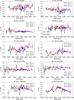 |
Fig. C.1 Circular polarization curves of the UMRAO data set (black circles) over-plotted against our results using both calibration methods A (red triangles) and B (blue squares) as described in Sect. 3.7. The comparison is performed over five sources with overlapping data sets, which were observed at 4.85 GHz (left column) and 8.35 GHz (right column). The data are available at the CDS. |
All Tables
Number of sources with at least one significant data point (S/N ≥ 3), mean uncertainty, and cadence of significant I, ml, mc, and χ measurements.
KS-test results (KS statistic D, and p-value) for the comparison between the σI,Q,U distributions for the 4.85 GHz data calibrated by the Müller method and our methodology.
Initial values of the Stokes Q and U instrument model parameters for the 4.85 GHz and 8.35 GHz receivers.
All Figures
|
Fig. 1 Schematic summary of the analysis sequence. Each analysis level is labeled with an index on the left and is discussed in the section noted on the right. The mean effect of each correction step is listed in Table 3. |
| In the text | |
|
Fig. 2 Example of the same sub-scan in all channels on the source 3C 286 at 4.85 GHz. The abscissa is the offset from the commanded position of the source. The LCP and RCP channel data sets are shown in the upper row while the COS and SIN data sets are shown in the lower row. The target source is ~11% linearly polarized. |
| In the text | |
|
Fig. 3 Stokes Qazi,elv (left column) and Uazi,elv (right column) data sets recorded at 4.85 GHz for the unpolarized, point-like source NGC 7027 in the two scanning directions; the azimuth in the top row and the elevation in the bottom row. Instead of the expected flat, noise-like pattern, the presence of spurious signals is clearly visible in both scanning directions. The instrumental polarization, calculated by the instrument model M, is shown in each panel with a smooth black line. The dashed blue lines mark the source position along the scanning direction. |
| In the text | |
|
Fig. 4 Generated Stokes Q and U instrument models in the two scanning directions, the azimuth in the top panels and the elevation in the bottom panels for (a) the 4.85 GHz (upper two rows) and (b) 8.35 GHz (lower two rows) receivers. The models were generated for 65 observing sessions. The variability of the plotted models is comparable to the respective errors of the fit. |
| In the text | |
|
Fig. 5 Example of the instrumental linear polarization correction for an elevation sub-scan at 4.85 GHz. The observed COS/SIN (or equivalently Qelv/Uelv) signals are shown with red in the middle and bottom rows, immediately below the LCP signal, while the corrected signals are shown with blue immediately below the RCP signal. The correction is performed by subtracting the expected instrumental polarization signals (smooth black lines) from the observed Qelv and Uelv data sets (2nd and 3rd column of the middle and bottom rows). The instrumental polarization signals are calculated by substituting the measured mean amplitude I, peak offset μ, and FWHM σ of the LCP and RCP signals (top row) in the instrument model M created for the given observing session. |
| In the text | |
|
Fig. 6 Degree of linear polarization (top panel) and polarization angle (bottom panel) of the source 3C 48 at 4.85 GHz before (red circles) and after (blue triangles) applying the instrumental linear polarization correction. The data correspond to 23 sub-scans of the source within a single observing session. The dashed red and dotted blue lines indicate the 1σ regions around the mean values of the uncorrected and corrected data sets, respectively. The mean, μ, and standard deviation, σ, values of the corresponding data sets are shown in the legend. |
| In the text | |
|
Fig. 7 Comparison between the Gaussian (left column) and Airy disk (right column) beam pattern models. The recorded data sets are shown in the top row with dark blue lines and the model fits with dashed, black lines. The corresponding fractional residuals, (data-model)/data, are given in the bottom row for a direct comparison between the models. |
| In the text | |
|
Fig. 8 Density plots of the measured offsets between the source position and the LCP, RCP, COS and SIN beam patterns for the 4.85 GHz receiver. The beam-squint can be clearly seen by the miss-alignment of the contour peaks (LCP: circle, RCP: upward-looking triangle, COS: square, SIN: downward-looking triangle). |
| In the text | |
|
Fig. 9 LCP (red circles) and RCP (black triangles) system temperature (Tsys) measurements versus the airmass (AM) for one observing session at 4.85 GHz. The AM range is split into a given number of bins and the data points with the lowest Tsys within each bin (filled markers) are used to fit the two lower envelopes (solid lines). Their slopes are practically identical, indicating that the atmospheric absorption does not influence the polarization of the transmitted radiation. |
| In the text | |
|
Fig. 10 Elevation-gain curves separately for LCP (red circles) and RCP (black triangles) data sets at 4.85 GHz. The similarity of the fitted parabolas indicates that the gravitational deformations do not affect the polarization measurements. |
| In the text | |
|
Fig. 11 Distributions of the circular polarization degree, mc, measurements at 4.85 GHz (top) and 8.35 GHz (bottom) for three observing sessions (solid black, dashed red and dotted blue lines). The non-zero average values, shown in the legend, indicate the presence of instrumental circular polarization. The mc measurements of the planetary nebula NGC 7027, in the corresponding sessions, are marked with arrows (in the bottom plot, two arrows overlap). |
| In the text | |
|
Fig. 12 Discrete correlation function (DCF) between the mc light curves of 4C +38.41 and CTA 102 before (cyan circles) and after the instrumental circular polarization correction using either method A (blue triangles) or method B (red squares) as described in the text. The corresponding 3σ significance levels are shown with dashed lines. |
| In the text | |
|
Fig. 13 Ratio r, calculated using both estimates of the circular polarization zero-level as described in method A for the 4.85 GHz (top) and 8.35 GHz (bottom) data sets. |
| In the text | |
|
Fig. 14 Discrete correlation function (DCF) between the |
| In the text | |
|
Fig. 15 mc measurements of NGC 7027 at 4.85 GHz (top) and 8.35 GHz (bottom) before (black circles) and after the instrumental circular polarization correction using both methods A (red triangles) and B (blue squares). |
| In the text | |
|
Fig. 16 Standard deviation distributions of the linear polarization degree, σml, polarization angle, σχ, and circular polarization degree, σmc, measurements at 4.85 GHz (top row) and 8.35 GHz (lower row). The 20th percentile, P20, of each standard deviation distribution is marked by a dotted line. The circular polarization data contain the measurements corrected with both methods A (solid black line) and B (dashed red line) as described in Sect. 3.7.1. |
| In the text | |
|
Fig. C.1 Circular polarization curves of the UMRAO data set (black circles) over-plotted against our results using both calibration methods A (red triangles) and B (blue squares) as described in Sect. 3.7. The comparison is performed over five sources with overlapping data sets, which were observed at 4.85 GHz (left column) and 8.35 GHz (right column). The data are available at the CDS. |
| In the text | |
Current usage metrics show cumulative count of Article Views (full-text article views including HTML views, PDF and ePub downloads, according to the available data) and Abstracts Views on Vision4Press platform.
Data correspond to usage on the plateform after 2015. The current usage metrics is available 48-96 hours after online publication and is updated daily on week days.
Initial download of the metrics may take a while.