| Issue |
A&A
Volume 609, January 2018
|
|
|---|---|---|
| Article Number | A5 | |
| Number of page(s) | 20 | |
| Section | Stellar structure and evolution | |
| DOI | https://doi.org/10.1051/0004-6361/201628363 | |
| Published online | 22 December 2017 | |
Improved model of the triple system V746 Cassiopeiae that has a bipolar magnetic field associated with the tertiary ⋆
1 Astronomical Institute of the Charles University, Faculty of Mathematics and Physics, V Holešovičkách 2, 180 00 Praha 8, Czech Republic
e-mail: This email address is being protected from spambots. You need JavaScript enabled to view it.
2 Astronomical Institute, Czech Academy of Sciences, 251 65 Ondřejov, Czech Republic
3 Department of Physics and Astronomy, The College of Charleston, Charleston, SC 29424, USA
4 University of Ege, Department of Astronomy & Space Sciences, 35 100 Bornova – İzmir, Turkey
5 Institute of Physics, Czech Academy of Sciences, Na Slovance 1999/2, 182 21 Praha 8, Czech Republic
Received: 22 February 2016
Accepted: 30 August 2017
Abstract
V746 Cas is known to be a triple system composed of a close binary with an alternatively reported period of either 25 4 or 278 and a distant third component in a 170 yr (62 000 d) orbit. The object was also reported to exhibit multiperiodic light variations with periods from 083 to 250, on the basis of which it was classified as a slowly pulsating B star. Interest in further investigation of this system was raised by the recent detection of a variable magnetic field. Analysing spectra from four instruments, earlier published radial velocities, and several sets of photometric observations, we arrived at the following conclusions: (1) The optical spectrum is dominated by the lines of the B-type primary (Teff 1 ~ 16 500(100) K), contributing 70% of the light in the optical region, and a slightly cooler B tertiary (Teff 3 ~ 13 620(150) K). The lines of the low-mass secondary are below our detection threshold; we estimate that it could be a normal A or F star. (2) We resolved the ambiguity in the value of the inner binary period and arrived at a linear ephemeris of
  . (3) The intensity of the magnetic field undergoes a sinusoidal variation in phase with one of the known photometric periods, namely 2503867(19), which we identify with the rotational period of the tertiary. (4) The second dominant photometric 10649524(40) period is tentatively identified with the rotational period of the broad-lined B-type primary, but this interpretation is much less certain and needs further verification. (5) If our interpretation of photometric periods is confirmed, the classification of the object as a slowly pulsating B star should be revised. (6) Applying an N-body model to different types of available observational data, we can constrain the orbital inclination of the inner orbit to ~60°<i1< 85° even in the absence of binary eclipses, and we estimate the probable properties of the triple system and its components.
Key words: binaries: close / stars: massive / stars: fundamental parameters / stars: individual: V746 Cas
Based on observations from the Ondřejov, Haute Provence, Bernard Lyot, ESO Hipparcos and Mercator Observatories.
© ESO, 2017
1. Introduction
While the nature of global magnetic fields in late-type stars with convective envelopes seems to be – at least in principle – understood as a consequence of the dynamo mechanism, the origin of organized magnetic fields detected in some O and B stars is less obvious. Given the large progress in the instrumentation allowing the detection of even weak magnetic fields, it is understandable that a very systematic search for the presence of magnetic fields among WR, O, B, and Be stars has recently been conducted by a large team of collaborators. This project, known as MiMES (Magnetism in MassivE Stars), was conducted between 2008 and 2013, and the first summary report was published by Wade et al. (2016). These authors report that unlike the magnetic fields of late-type stars, the magnetic fields of hot stars do not show any clear correlations with basic stellar properties such as their mass or rotation rate. We note that the realisation has grown in recent years that a large portion of O and B stars are binaries or even multiple systems, which must have significant impact on the understanding of their properties (see, e.g. Chini et al. 2012; de Mink et al. 2013). The role of multiplicity in the magnetism of hot stars is worth consideration. Recently, Neiner et al. (2014) reported one preliminary result of the MiMES survey: the discovery of a magnetic field of the triple system V746 Cas. Since the properties of this system were not well known, we were motivated to this study.
V746 Cas (HD 1976, HR 91, BD+51°62, HIP 1921, Boss 67) is a bright (V = 5 6) B5 IV star. Its radial-velocity (RV) variations were discovered by Adams (1912) and confirmed by Plaskett & Pearce (1931). Blaauw & van Albada (1963) derived RVs from a new series of McDonald spectra and published the first orbital elements; see Table 1. In addition to their spectra, they also used the Dominion Astrophysical Observatory (DAO) spectra. Abt (1970) published six previous Mt. Wilson RVs, which partly overlap with those published by Adams (1912). Abt et al. (1990) measured RVs of 20 new KPNO spectra and published another set of elements, deriving a period of 2544 ± 003. Their solution is based solely on the KPNO RVs, but the authors claim that it also fits the previous Mt. Wilson, DAO, and McDonald RVs. McSwain et al. (2007) analysed their 15 new KPNO RVs along with earlier published data and found two comparable periods near 254 and 276. We note that these two periods are 1 yr aliases of each other. McSwain et al. (2007) preferred the shorter period and obtained another solution, this time based on most of previously published RVs, which is also given in Table 1.
Previously published orbital solutions for the V746 Cas close binary.
The first attempt to detect the spectral lines of the secondary was reported by Gómez & Abt (1982). They studied 160 Å long CCD spectra in two wavelength regions: one containing He i 5876 Å and the Na i doublet at 5889 and 5895 Å, and the other containing the Si ii doublet at 6347 and 6371 Å, the Ne i 6402 Å line, and several Fe ii, Fe i, and Ca i lines, to be able to restrict the possible spectral class of the secondary. They did not show the actual line profiles and published only a few comments. They concluded that the spectral type of the secondary must be earlier than F6, and suspected a possible weak secondary component in the He i 5876 Å line.
V746 Cas is also the brighter member of the visual system ADS 328. Doboco & Andrade (in Doboco & Ling 2005) derived the orbit of the wide pair with a period of 169.29 yr (61 832 d), semimajor axis 0.̋214, eccentricity 0.163, inclination  , argument of periastron
  and periastron passage at 1955.06 (JD 2 435 130). The distant component B is by some 09 fainter than V746 Cas.
The light variability of V746 Cas in the range from 554 to 556 was discovered by the Hipparcos team (Perryman & ESA 1997), and several investigators reported the presence of two principal periods, 1065 and 2504, and alternatively a few additional periods as well (for instance Waelkens et al. 1998; Andrews & Dukes 2000; De Cat et al. 2007; Dukes et al. 2009, see Sect. 4 for a more detailed account). They all classified the object as a slowly pulsating B-type star (SPB). Before the light variability was discovered, Glushneva et al. (1992) published spectrophotometry of V746 Cas and several other stars and suggested that V746 Cas could serve as a secondary spectrophotometric standard.
Neiner et al. (2014) reported the discovery that the line spectra of V746 Cas are composed of a narrow component, for which they found clear signatures of a magnetic field, and a broad component that is much more variable in RV. They identified the narrow lines and the magnetic field with the primary and the broad-line component with the secondary of the 254 binary, concluding that the lines of the distant tertiary are not seen in the spectra. They allowed, however, that the narrow-lined star might also be the visual tertiary or a combination of the primary and tertiary.
Our initial motivation for this study was to resolve the remaining ambiguity in the value of the orbital period. We started to collect new CCD spectra in the red spectral region. Their subsequent analysis led us to a more complex investigation and hopefully to a better understanding of this remarkable triple system, which we report here.
2. Available observational data and their reductions
2.1. Spectroscopy
Our observational material consists of 41 Ondřejov CCD spectra secured in 2014–2015 (S/N 160–300; three underexposed spectra with 27, 37, and 100), 17 OHP Aurelie spectra with an S/N of 130–230, the first one of 36 only (Gillet et al. 1994), which were obtained and studied by Mathias et al. (2001), 3 archival OHP Elodie spectra with S/N 270–280 in the red parts of the spectra (Moultaka et al. 2004), and 13 publicly available echelle spectra from the Bernard Lyot telescope with an S/N greater than 200 in the red parts of the spectra (Petit et al. 2014). The initial reduction of all Ondřejov spectra (bias subtraction, flat-fielding, creation of 1D spectra, and wavelength calibration) was carried out in IRAF. For the Bernard Lyot and OHP Elodie spectra, extracted from public databases, we adopted the original reductions, verifying that the zero-point of the wavelength scale was corrected via telluric lines, as was the case for the Ondřejov spectra. This was more complicated with the Aurelie spectra, which are not available from public archives. P. Mathias kindly provided us with the old DAT tapes, which were reconstructed in Prague. Their new reduction was carried out with the help of simple dedicated programs, the wavelength calibration being carried out with the program SPEFO (Horn et al. 1996; Škoda 1996), namely the latest version 2.63 developed by J. Krpata. Median values of each corresponding sets of offsets and flat spectra were used.
Rectification and removal of residual cosmics and flaws for all sets of spectra were carried out in SPEFO.
We first extracted the red parts of the Elodie and Bernard Lyot spectra (~6360–6740 Å) to have the same spectral region as is covered by the Ondřejov spectra. One Ondřejov spectrum is shown in Fig. 1. As was previously noted by Neiner et al. (2014), the line profiles are not symmetric but contain broad and narrow components, the broad component varying in RV over a wide velocity range. The profiles might also be affected by subfeatures that are related to rapid light and line-profile variations and move across the line profiles as a result of stellar rotation. For all Elodie and Bernard Lyot spectra, we also extracted the blue, green, and yellow parts of the spectra over the wavelength range from 4000 to 6360 Å. We also extracted the Aurelie spectra, which cover the wavelength range from 4095 to 4155 Å.
Finally, we also collected RV measurements obtained by several investigators and published in the literature. The journal of all available RVs is listed in Table 2 and all individual RVs are presented in Table A.1 for the data from the literature. When they were not available in the original source, we converted the observation dates into HJDs. For brevity, we use reduced Julian dates
 throughout. Abt (1970) published six RVs from Mount Wilson secured between December 1910 and November 1921. They include RVs published by Adams (1912), with the exception of the very first observation, which was secured on 1910 December 21. We therefore adopted the first RV from Adams (1912) and all remaining Mount Wilson RVs (spg. 1) from Abt (1970).
 |
Fig. 1 Top: Ondřejov spectrum taken on RJD 56 928.3090 is shown, and several stronger spectral lines are identified. All sharp lines in the vicinity of Hα are telluric or weak interstellar lines. Bottom: the Haute Provence Aurelie spectrum taken on RJD 51 011.5748, the stronger lines are again identified. |
Journal of RV data sets.
2.2. Standard RV measurements
To resolve the problem of the true orbital period and to obtain reliable orbital elements, we first tested several techniques of RV measurements. For the most numerous set of the red spectra, we measured the two strongest lines, Hα and He i 6678 Å, in SPEFO. This program displays direct and flipped traces of the line profiles superimposed on the computer screen that the user can slide to achieve a precise overlapping of the parts of the profile whose RV is to be measured. We separately measured the line cores and outer line wings. We note that two of the Ondřejov spectra (RJDs 56 920 and 57 228) are underexposed and we were only able to measure the RVs of the wings of Hα. These RV measurements are listed in Table A.2. For the Aurelie spectra, we also measured RVs of the broad wings of the He i 4144 Å line, and these measurements are listed in Table A.3 in Appendix A.
While the uncertainty of the SPEFO measuring procedure alone seems small (of the order of a few km s-1), as determined from three independent measurements, there are three additional sources of uncertainties: photon noise, systematics arising from the rectification, and systematics from line blending. The latter is probably not critical for RVs of a particular spectral line, but they may dominate the uncertainty budget for a mean RV from several spectral lines (as discussed below). In any case, the total uncertainty is higher than the formal rms errors and might reach up to 10 km s-1 in the least favourable cases.
For the Elodie and Bernard Lyot spectra, we also measured RVs of the following stronger lines in SPEFO: He i 4009, 4143, 4471, 4713, 4922, 5016, 5047, and 5876 Å, C ii 4267 Å, and Mg ii 4481 Å. We did not use the He i 4026 Å, 4120 Å, and 4387 Å lines, since the first is affected by an inter-order jump in all Bernard Lyot spectra, while the profiles of the other two lines are affected by strong blends in their neighbourhood. Finally, for the Aurelie spectra we measured RVs of Hδ and He i 4143 Å.
 |
Fig. 2 Dynamical spectra plotted vs. orbital phase of the 25 |
2.3. Photoelectric observations and their homogenisation
There are three principal sets of photoelectric observations suitable for period analyses:
-
1.
The Hipparcos Hp observations (Perryman &ESA 1997);
-
2.
the uvby observations from the Four-College APT secured by one of us; a subset of these observations has previously been analysed by Dukes et al. (2009); and
-
3.
the Geneva 7-C observations obtained and studied by De Cat et al. (2004) and De Cat et al. (2007).
One of us, R.J. Dukes, was able to recover the APT uvby observations, or more precisely, a more numerous data set than was used in his published studies. It was deemed useful to repeat the period analysis with a complete and homogenised set of the data. The yellow-band observations (Hp and Geneva V magnitudes converted into Johnson V, and Strömgren y) are the most numerous and represent the best set for the analysis. More details on the data processing and their homogenisation can be found in Appendix C, where the journal of these observations is also listed in Table C.1. After the removal of data from non-photometric nights, we are left with 2060 individual yellow-band observations spanning an interval of nearly 9800 d.
3. Towards true orbital periods of the system
Figure 2 shows dynamical spectra for the Hα and He i 6678 Å line versus phase of the 25416 period. The orbital motion in the line wings of both lines is clearly visible. In contrast, the line cores do not exhibit clear RV variations with the same amplitude. We also note that there is no indication of an antiphase RV variation expected for the secondary in the 25416 orbit. This means that the bulk of the line cores is not associated with the primary, as suggested by Neiner et al. (2014), but with the tertiary of the visual orbit.
As explained above, we measured RVs separately for the broad and narrow parts of the Hα and He i 6678 Å lines. We immediately noted, in accord with Neiner et al. (2014), that the range of RV variations is much smaller for the narrow parts of the lines, and we verified that the RVs of the wide parts of the lines vary with the known ~ 25.4 d period.
The SPEFO RVs of the line cores of the Balmer lines seemingly follow the 25.4 d RV curve of the wide parts of the lines, in phase with the wide wings, but with a strongly reduced amplitude. This implies that they do not belong to the secondary in the 25.4 d orbit but to the distant tertiary, with a nearly constant RV. Their apparent RV changes are caused only by the strong line blending of the lines of the primary and tertiary.
3.1. Period analysis of RVs
To resolve the question of the true value of the orbital period of the closer pair, we calculated PDM periodograms (Stellingwerf 1978) for individual data subsets. They are shown in Fig. 3. It is immediately seen that neither the Blaauw & van Albada (1963) nor the McSwain et al. (2007) RVs alone are able to restrict the value of the orbital period. Blaauw & van Albada (1963) were obviously aware of the limitations of their data set since they estimated the uncertainty of the 278 period to be as much as one day. The time interval covered by their own observations is shorter than two orbital periods. We also note that the first data set from spectrograph 1, although it spans a long time interval, is probably of limited accuracy and cannot be used to determine a unique period.
 |
Fig. 3 Stellingwerf (1978)θ statistics periodograms for several data sets of RVs published by various authors, and the SPEFO RVs of the outer wings of the Hα and Hδ lines. |
Only observations by Abt (1970) and our new RVs are numerous enough to identify the true orbital period. Their periodograms are mutually similar. The dominant period of 25416 (f = 0.0393 c d-1) and its first harmonics are clearly visible. A smaller minimum at 0.0360 c d-1 corresponds to a 1 yr alias of the 25416 period.
3.2. Linear ephemeris for the inner-orbit period
To obtain as precise a value of the orbital period P1 of the inner binary as possible, we derived some trial orbital solutions with the program FOTEL (Hadrava 1990, 2004a). We first calculated an orbital solution based on our new SPEFO RVs. The semiamplitude for the He i 6678 Å RVs is higher than that obtained from the Hα RVs. It is a well-known effect for early-type stars that the lines with appreciably Stark-broadened wings like the Balmer lines give lower RV amplitudes and are not suitable for the determination of true orbital elements (e.g. Andersen 1975; Andersen et al. 1983). This clearly represents another complication on the way to obtaining realistic binary properties.
Since our first task is, however, to derive the correct value of the orbital period, we adopted the SPEFO Hα RVs and Hδ RVs for the Aurelie spectra, which give a semiamplitude closer to those found by previous investigators; see Table 1. We combined them with all RVs from the literature and ran a solution in which we allowed the calculation of individual systemic velocities (γs) for individual data sets. Using the rms errors of individual sets, we derived their weights inversely proportional to the squares of the corresponding rms errors. Investigating the phase plots, we found that the RVs of spectrograph 1 (Mt. Wilson) probably refer to a combination of the broad and narrow parts of the line profiles and cannot contribute meaningfully to constrain the orbital period.
Exploratory FOTEL solutions for RVs from the literature and from our red spectra.
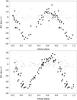 |
Fig. 4 Top: a phase plot of all file 2 to file 5 RVs (i.e. data from the literature). Bottom: a phase plot of all our new file 6 to file 9 RVs. SPEFO Hα and Hδ RVs were used for the new spg. 6 to 9 spectra. Small dots denote the O–C residuals from the orbital solution. All RVs in the two lower panels were corrected for the difference in γ velocities, adopting γ of the most numerous file 9 as the reference. In all plots, the orbital period of 25 |
We then calculated a joint solution for all weighted RVs from spgs. 2–8 (see the first solution in Table 3), and we adopted the orbital period from this solution  (1)Phase plots for this joint solution are shown in Fig. 4, separately for the RVs from the literature and for our new Hα and Hδ RVs.
Keeping the orbital period fixed, we then derived two other solutions, this time based on our new He i 6678 Å RVs from spgs. 6–9 and using alternatively the RV set based on the Gaussian fits and on the SPEFO RVs. The results are also listed in Table 3. The elements show that it is not easy to choose the correct value of K1 and the mass function. The semiamplitude and eccentricity differ for the individual solutions, depending on the line(s) measured and also on the measuring technique. A part of the problem is the fact that almost all spectral lines are to some extent affected by neighbouring blends.
We also tried to disentangle the lines of the system components using the KOREL program (Hadrava 1995, 1997, 2004b). However, since the spectra at our disposal cover only one-tenth of the visual orbit for the He i 4143 Å line and even less for the other spectral lines, the semiamplitudes of the bodies in the outer orbit could not be meaningfully converged and we have no firm clue how to fix them. We only verified that no trace of the secondary could be found. In our experience, this implies that the secondary must be for more than three magnitudes fainter than the combined light of the primary and tertiary.
3.3. Speckle-interferometry and the visual orbit
Adding one speckle-interferometric observation from 2007 (Mason et al. 2009) to the existing set of 37 observations of V746 Cas, we were able to derive a new visual orbit of the third body, but our preliminary solution confirmed the orbit published by Docobo and Andrade (see Doboco & Ling 2005). For reference, it is summarised in Table 4. The reported uncertainties are the nominal ones, corresponding to a single local minimum of the respective χ2. However, the values of P2 and e2 seem to be strongly correlated. Moreover, they strongly depend on the five previous astrometric observations from the beginning of the 20th century. Their real uncertainty can probably be greater than 0.02 arcsec, which we assumed for them.
Improved visual orbit of the V746 Cas tertiary.
4. Nature of the rapid photometric variations
4.1. Overview and analysis of previous results
Frequencies and periods of light variations of V746 Cas found by various investigators.
Table 5 provides an overview of various frequencies of light variations of V746 Cas reported by several investigators. There seems to be no doubt about the two principal frequencies, detected by all investigators, 0.939 and 0.399 c d-1. Notably, Mathias et al. (2001) were unable to find any spectroscopic signatures of these two frequencies in their Aurelie spectra covering the wavelength interval from 4085 to 4155 Å. The authors state, however, that all their spectra have S/Ns lower than 140. Two groups, De Cat et al. (2004) and Dukes et al. (2009), reported another frequency, 0.799 c d-1. De Cat et al. (2004) denoted it as a possible alias. We note that it is an exact harmonics of the 0.399 c d-1 frequency. In our opinion, this indicates that the light curve with the 0.399 c d-1 frequency deviates from a sinusoidal shape. Therefore, the 0.799 c d-1 frequency is not an independent frequency. Another weak frequency of 1.20346 c d-1 reported by De Cat et al. (2007, which in our opinion could be the second harmonics of 0.399 c d-1 could not be confirmed by Dukes et al. (2009), who analysed their own Strömgen uvby photometry from the Four College Automatic Photoelectric telescope (APT) along with the Hp and Geneva 7-C photometries. They found a frequency of 0.9309 c d-1, however, which is quite close to f1 = 0.939 c d-1. We note that 0.9390 and 0.9309 c d-1 mutually differ for one-third of the frequency of a sidereal year, so we suspect that the 0.9309 cd-1 frequency is an alias. The above facts led us to suspect that the light changes of V746 Cas are modulated only by two independent periods.
4.2. New period analysis of available photometry
For the purpose of the period analysis, we subtracted seasonal mean values from all data to remove possible slight secular variations of either instrumental systems of the telescopes or true small secular changes (see Appendix C for details). We used the programs PERIOD04 (Lenz & Breger 2005) and FOTEL for the modelling and fits. We found that the longer, non-sinusoidal period of 2.5 d has larger amplitudes for the second and fifth harmonics as well (periods 125 194, and 050 077), which were then included into fits. Inspecting cases with more observations within short time-intervals like 0.03 d, we conclude that in all three data sets there are cases when the rms error of single observations exceeds 0007. The rms error of the fit is only slowly decreasing when more frequencies are added, and it remains on the 0007 level.
We arrive at the following ephemerides for the 1065, and 2504 periods:  Binary eclipses can also be safely excluded from the available photometry (see Fig. 5). Our simulations of the light curve for the 254 orbit with the program PHOEBE 1 (Prša & Zwitter 2005) for plausible values of the stellar radii (see below) then show there is a rather strict upper limit for the orbital inclination, i1 ≤ 85°.
 |
Fig. 5 All yellow-band photometric observations prewhitened for both the 1 |
4.3. Periodic variations of the magnetic field
We tried to determine whether the observed variations of the magnetic field found by Neiner et al. (2014) might not be related to the known photometric changes. We quickly found that the magnetic field indeed varies with the longer of the photometric periods, 250 387; see Fig. 6.
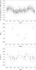 |
Fig. 6 Phase plots for the 2 |
A sinusoidal variation of the magnetic field intensity is commonly interpreted as a dipole field inclined to the rotational axis of the star and varying with the stellar rotational period. Neiner et al. (2014) associated the magnetic field with the narrow-line component, which they considered to be the primary, but which is – as we have shown here – the distant tertiary component moving in the long orbit with the 254 binary.
In the bottom panel of Fig. 6 we also plot the Gaussian-fit RVs of the narrow component of He i 6678 Å (i.e. RVs of the magnetic-field tertiary) line vs. phase of the 2504 period. The scatter is rather large, but the RV variations clearly show some similarity to the light changes. This could be due to the corotating structures related to the magnetic field of the tertiary. We mention this to alert future observers that it might be rewarding to obtain systematic whole-night series of spectra at high resolution to verify the reality of the phenomenon and possibly to apply techniques such as Doppler imaging if the phenomenon is confirmed to be real.
 |
Fig. 7 Phase plots for the 1 |
4.4. Rapid line-profile changes of the primary?
If some rapid line-profile changes are also present in the spectra of the primary, they could manifest themselves as additional RV disturbances, overlapped over the orbital RV changes. While the technique of the settings on the outer line wings in SPEFO might tend to mask such changes (while affecting the true RV amplitude), such disturbances should be best detected in the Gaussian fits, which use two fixed Gaussian line profiles, mutually moved only in RV. We therefore inspected the O–C RV residuals from the 254 orbit for the Gaussian He i 6678 Å RVs based on repeated measurements. In Fig. 7 we compare the plot of these RV residuals with the plot of yellow-band photometry prewhitened for the 250 387 period. There is some indication of sinusoidal residual RV changes with the photometric period of 1065, especially for RVs with lower rms errors. The modulation is nicely seen in the subset of Aurelie high-S/N and high-resolution spectra. While it is clear that the ultimate confirmation may only come from new whole-night series of high-resolution spectra, we do believe there is a reason to identify the 1065 period with the rotational period of the primary. The modulation of measured RVs could be caused by some structures on the surface of the primary, moving across the stellar disk as the star rotates. We note that there is growing evidence for rotational modulation for a number of B stars from the photometry obtained by the Kepler satellite and by ground-based surveys (see, e.g. McNamara et al. 2012; Nielsen et al. 2013; Kourniotis et al. 2014; Balona et al. 2015, 2016).
5. Initial estimates of the basic physical elements of the system
5.1. Radiative properties of the primary and tetriary
To determine the radiative properties of the two dominant components, we used the Python program PYTERPOL, which interpolates in a pre-calculated grid of synthetic spectra. Using a set of observed spectra, it tries to find the optimal fit between the observed and interpolated model spectra with the help of a simplex minimization technique. It returns the radiative properties of the system components such as Teff, v sin i or log g, but also the relative luminosities of the stars and RVs of individual spectra1. The function of the program is described in detail in Nemravová et al. (2016).
In our particular application, two grids of synthetic spectra, Lanz & Hubený (2007) for Teff > 15 000 K, and Palacios et al. (2010) for Teff < 15 000 K, were used to estimate basic properties of the primary and tertiary for all 16 Aurelie, 3 Elodie, and 13 Bernard Lyot high-S/N spectra. The following spectral regions containing numerous spectral lines, but avoiding the inter-order transitions and regions with stronger telluric lines, were modelled simultaneously:
Relative component luminosities were fitted separately in four spectral bands: 4000–4280 Å, 4308–4490 Å, 4700–5025 Å, and 6670–6690 Å. Uncertainties of radiative properties were obtained through Markov chain Monte Carlo (MCMC) simulation implemented within emcee2 Python library by Foreman-Mackey et al. (2013). They are summarised in Table 6. We note that in contrast to the N-body model, which we use below for the final estimate of the most probable properties of the system, PYTERPOL derives the RV from individual spectra without any assumption about orbital motion. It is therefore reassuring that when we allowed for a free convergence of the orbital period in a trial solution based on the PYTERPOL RVs, we arrived at a value of 254156(13), in excellent agreement with the value of ephemeris (1) based on all available RVs.
5.2. Additional properties of the primary
All available MKK spectral classifications of V746 Cas summarized in the SIMBAD bibliography, including a recent one by Tamazian et al. (2006) based on high-resolution spectra, agree on the spectral type B5 IV. Dereddening of the mean all-sky standard UBV magnitudes from Hvar (see Table C.1) gives V0 =543, (B−V)0 = −0170, (U–B)0 = −0635, and E(B−V) = 0055, which corresponds to a B4-5IV star after the calibration by Golay (1974).
We can then use the observed Hipparcos parallax p of V746 Cas to further constrain the primary. According to the improved reduction (van Leeuwen 2007a,b),  . Assuming the above mentioned V0 = 543 for the whole system, the observed magnitude difference between the primary and tertiary and neglecting the light contribution from the unseen secondary, we arrive at
  82 for the primary. Using the above-mentioned range of the possible values of the parallax, 0.̋00263 to 0.̋00394, we obtain
  08 and −120, respectively. The bolometric corrections for the considered range of the effective temperature of the primary are from −1433 to −1557 so that the extreme allowed values of the bolometric magnitude of the primary
  are −263 to −364.
Radiative properties of the V746 Cas primary and tertiary derived from a comparison of selected wavelength segments of the observed and interpolated synthetic spectra of the primary and tertiary.
If 1065 is the rotational period of the primary, then for v sini1 = 179 km s-1, derived from the PYTERPOL solution for the primary, R1 ≥ 2πvsini/P = 3.77 R⊙. For instance, if i1 = 70°, we obtain R1 = 4.01 R⊙. For the expected range of the primary mass, this would imply log g = 3.98 to 4.04 [cgs] for the primary, which is slightly offset at the 2.5σ level with respect to the range deduced from the fit by synthetic spectra (Table 6). We note, however, that the log g values are very sensitive to an accurate placement of the continuum, which is especially difficult for Balmer lines from the echelle spectra. On the other hand, if the true rotational period is a photometric double-wave curve with a period twice longer, that is, 2130, we would obtain log g = 3.38 to 3.44 [cgs]; again offset from the nominal range. This would also correspond to significantly larger radius R1 = 8.02 R⊙ and an even lower upper limit of i. Given all the uncertainties involved, however, both possibilities need to be kept in mind.
5.3. Tertiary component
The more recent estimates of the magnitude difference between the close binary and tertiary from astrometry (Perryman & ESA 1997; Mason et al. 2009) agree on  . The relative luminosities of the primary and tertiary estimated with PYTERPOL (see Table 6) imply
  , in remarkable agreement with the astrometric estimates. This once more confirms our identification of the narrow-line component seen in the spectra with the tertiary.
Using the v sini3 = 72 km s-1 estimated from the PYTERPOL solution for the tertiary and adopting the 2504 period as its period of rotation, we can similarly estimate the radius of the tertiary R3 ≥ 3.56 R⊙. Assuming that the inclination of the rotational axis of the tertiary is identical with the orbital inclination of the outer orbit 64°, we estimate log g from 3.90 to 4.01 for it. This agrees quite well with the observed range of log g from the line-profile modelling.
 |
Fig. 8 Evolutionary tracks in effective temperature Teff vs. surface gravity log g plots, including pre-MS (thin line), MS, and SGB phases (thick line). The horizontal and vertical dotted lines correspond to the allowed 1σ ranges of the respective parameters, according to Table 6. The top panel shows the primary component of V746 Cas for the two values of its mass m1 = 5.6 M⊙ and 6.7 M⊙. The bottom panel shows the tertiary for m3 = 4.6 M⊙ and 6.0 M⊙. |
5.4. Component masses
In order to preliminarily estimate the component masses, we calculated evolutionary tracks using the Mesastar program (Paxton et al. 2015) and compared them with the observed range of the values of Teff and log g, deduced from the line-profile fits, in Table 6. In all cases we assumed a helium abundance Y = 0.274, metallicity Z = 0.0195 (i.e. very close to the standard values of Caughlan & Fowler 1988), and mixing length parameter α = 2.1. We also accounted for element diffusion, Reimers red giant branch (RGB) wind with η = 0.6, Blocker AGB wind with η = 0.1, even though neither is very relevant on the zero-age main sequence (ZAMS). Semiconvection and convective overshooting were both switched off. The maximum output time step was Δt = 105 yr to resolve the terminal main sequence (TAMS). Mesastar program, rev. 8845 (Paxton et al. 2015), was used for these computations.
From the comparison presented in Fig. 8, we can estimate the mass of the primary to be from m1 = 5.6 to 6.7 M⊙ (1σ range). We verified that the evolutionary tracks in the considered region close to the TAMS are not overly sensitive to the value of metallicity. For Z = 0.04, the corresponding mass range changes by as much as 0.1 M⊙; lower metallicities are not likely for relatively young stars. The same is true for the mixing-length parameter α or the semiconvection parameter αsc, since both stars are in a radiative equilibrium. For instance, α = 1.6 or αsc = 0.01 lead to essentially the same results. For the overshooting parameters fov = 0.014 and f0 = 0.004 (i.e. within the range discussed in Herwig 2000), the evolution around the TAMS is notably different, nevertheless, the range of masses would be shifted only slightly upwards, by less than 0.1 M⊙,
A similar analysis for the tertiary component led to the mass m3 = 4.6 to 6.0 M⊙. Within the uncertainties, the primary and tertiary stars can even be equally massive and have very similar effective temperatures. The similarity of the primary and tertiary is also supported by the fact that their relative luminosities over the whole optical range seem to be the same; see Table 6.
6. N-body model of the V746 Cas system
6.1. Formulation
To analyse all available observational data in the most consistent way, we attempted to use the N-body model of Brož (2017), which was recently developed and successfully applied to the ξ Tauri quadruple system (Nemravová et al. 2016). Here, we used a significantly extended version of it. While a detailed technical description is given in the latter paper, we repeat here a subset of equations relevant for our problem:
![Mathematical equation: \begin{eqnarray} &&\ddot{\vec{r}}_{{\rm b}i} = -\sum_{j\ne i}^{N_{\rm bod}} {Gm_j\over r_{ji}^3}\,\vec{r}_{ji} + \vec{f}_{\rm tidal} + \vec{f}_{\rm oblat} + \vec{f}_{\rm ppn} , \\ &&I_\lambda' = \sum_{j=1}^{N_{\rm bod}} {L_j\over L_{\rm tot}} \,I_{\rm syn}\!\left[\lambda\left(1-{v_{z{\rm b}j+\gamma}\over c}\right), T_{{\rm eff}\,j}, \log g_j, v_{{\rm rot}\,j}, {\cal Z}_j\right], \\ &&F_V' = \sum_{j=1}^{N_{\rm bod}} \left({R_j\over d}\right)^{\!2} \int_0^\infty F_{\rm syn}\!\left[\lambda, T_{{\rm eff}\,j}, \log g_j, v_{{\rm rot}\,j}, {\cal Z}_j\right] f_V(\lambda) {\rm d}\lambda , \\&& m_V' = -2.5\log_{10} {F_V'\over F_{V{\rm calib}} \int_0^\infty f_V(\lambda){\rm d}\lambda}\,,~~~ \end{eqnarray}](/articles/aa/full_html/2018/01/aa28363-16/aa28363-16-eq140.png)
where the notation is as follows. The index i always corresponds to observational data, j to individual bodies, Nbod = 3 is the number of bodies, rb barycentric coordinates, m component mass, ftidal, foblat and fppn contributions from tidal, oblateness, and parametrized post-Newtonian (PPN) accelerations, which are included for the sake of completeness, even though they are negligible in the V746 Cas system; Iλ, Isyn normalized synthetic spectrum (intensity) of the whole system and component, with appropriate Doppler shifts, L,Ltot component luminosity and the total luminosity, Teff effective temperature, log g surface gravity [in cgs], vrot projected rotational velocity,  metallicity, Fsyn absolute monochromatic flux (in erg s-1 cm-2 cm-1 units) for any of the standard UBVRIJHK or non-standard bands, FVcalib calibration flux, and fV(λ) filter transmission function. Both normalized and absolute synthetic spectra were interpolated on-the-fly by PYTERPOL, as described in Nemravová et al. (2016). For the absolute spectra, the grids BSTAR (Lanz & Hubený 2007) and PHOENIX (Husser et al. 2013) were used.
Synthetic data and observation are compared by means of a combined χ2 metric  (8)with individual contributions defined as

where xp,yp denote 1 + 2 photocentric sky-plane coordinates, σsky major, minor uncertainty of the astrometric position, φellipse position angle of the respective ellipse, R(... ) the corresponding 2 × 2 rotation matrix, σsyn uncertainty of the normalized intensity, σsed uncertainty of the spectral-energy distribution, and  minimum and maximum allowed masses. The last term is an artificial function with a sufficiently steep and smooth behaviour; the high exponent prevents the simplex from drifting away. Optionally, we can use weights w to enforce a convergence for selected less-numerous data sets (e.g. with wsky = 10).
 |
Fig. 9 Subset of synthetic spectra |

6.2. Application to V746 Cas
The number of free parameters in our model is Lfree = 26; namely the masses mj, orbital elements of the two orbits Pj, ej, ij, Ωj, ωj, Mj, systemic velocity γ, distance d, gravitational acceleration log gj, effective temperatures Teff j, and projected rotational velocities vrot j. Radii are thus dependent quantities computed as  . As usual, the parameter space is very extended and we can expect a number of local minima. As reasonable starting points, we used the results of previous observation-specific models. We then employed a simplex algorithm for the minimisation, with various starting points and several restarts. We also verified the results by simulated annealing, even though neither of the algorithms can guarantee that the true global minimum was found.
We used a complete observational data set: (i) 37 speckle-interferometric and astrometric observations of the third body, including some older and rather uncertain ones; (ii) 72 spectra from the Elodie, Aurelie, Lyot, and Ondřejov datasets; this would represent 184 666 individual data points, but for our analysis we used 21 506 mean points in order to have a faster computation with a comparable resolution of all spectra; (iii) 93 spectral-energy distribution measurements from Hvar, Geneva and Glushneva et al. (1992). For the last data set we had to perform dereddening, assuming AV = 3.1 E(B−V) relation, E(B−V) = 0.055, and the wavelength dependence from Scheffler & Elsaesser (1987), Table 4.1.
On the other hand, we did not use radial velocities, as these are derived quantities possibly affected by some systematics, but rather the rectified spectra directly. We incorporated the same spectral regions, unaffected by any stronger telluric lines as in Sect. 5.1. Our approach is even better than using Pyterpol alone (which fits a single spectrum at a time), because the orbital motion is simulated by the N-body model, which links the spectra observed at different times. As a consequence, we are more sensitive to uncertainties and systematics of the rectification procedure, which would otherwise be hidden.
Osculating orbital elements at the epoch T0 = 2 454 384.65 and radiative parameters derived for V746 Cas using the nominal N-body model.
We encountered two serious problems, which required some modifications of the program. First, the secondary is practically unconstrained, except for the radial motion of the primary. Its convergence is thus impossible and we used the Harmanec (1988) relations instead, that is to say, we used only its effective temperature Teff 2 as a free parameter and computed the remaining ones, as log m2(X), log R2(X), log g2(X), where X ≡ log Teff 2, to constrain the secondary as a main-sequence star. If the secondary becomes too hot in the course of convergence, it will become visible in the synthetic spectra, of course.
Another problem arises from missing direct estimates of the radii R1 and R3 (there are no eclipses, no spectro-interferometry). We experienced a tendency to converge towards unrealistic hot subdwarfs and therefore had to use a mass constraint inferred from Mesastar modelling, in particular  , which corresponds to a 3σ lower limit.
Finally, a technical note: we prefer to inspect first the χ2 values, which are not reduced, that is, not divided by the respective number of degrees of freedom ν. This gives a better chance to search for possible reasons of systematic errors (or model deficiencies).
We also prefer to use the nominal uncertainties in our modelling (not directly the “realistic” ones) because otherwise we would not be sensitive to any systematics at all; they would be completely hidden in large σs and we might be falsely satisfied with the model.
6.3. Nominal model
The nominal model is presented in Table 7 and Fig. 9. Its total χ2 value seems too high, χ2 = 157 756, that is, much higher than the corresponding number of degrees of freedom ν ≡ Ndata−Lfree = 21 647, the reduced  and the resulting probability is thus essentially zero. However, we explain the mismatch as follows. While the
  contribution seems perfectly reasonable and it is indeed not difficult to reach the value as low as Nsky, it may become larger in the course of fitting because the other data sets are much more numerous and are likely affected by systematics.
The systematics in  are probably caused by the rectification procedure, even though it was performed as carefully as possible. For example, we sometimes see differences for a given spectrum that is surrounded by two or more spectra that are fitted well enough. The same is true for individual lines in a single spectrum, for instance, we have a good fit of the C ii and Mg ii lines, while Hγ (with its extended wings) and He i are somewhat offset. In principle, we cannot exclude the presence of rapid line-profile variations, but a self-consistent model would be needed for them, otherwise such unconstrained variations could explain any departures from the model (including any systematics).
The value of  seems also higher than expected. This is probably caused by systematics in calibrations of the absolute fluxes (even the Hvar and Geneva photometry from Table C1 differ by more than 3σ). Alternatively, a significant systematic uncertainty can be hidden in the dereddening procedure (see below). If we accept the arguments above and the high value of the nominal χ2, then 1σ probability level would correspond to an increase of up to 158 659, and 3σ to 162 201.
Parameter uncertainties can be obtained by a bootstrap or χ2 mapping. In this case, we used the latter method, with the notion that the respective uncertainties correspond to a local minimum only. Several correlations are still present in the model, however. In particular, a lower inclination i1 usually requires a higher mtot. A similar correlation exists between the distance d and mtot. Moreover, there is a non-zero possibility of a long orbit of the tertiary, with P2 ≃ 211 000 d, a high eccentricity e2 ≃ 0.65, and small d, with only marginally worse  , but the total χ2 is then relatively large.
Parameters derived for V746 Cas with the N-body model but without spectral data in the vicinity of the Balmer lines Hβ, Hγ, and Hδ, which are prone to several instrumental problems and rectification systematics (on the other hand, Hα from the Ondřejov linear spg. 9 was included).
We emphasize that the results can differ from previous observation-specific models. In Table 7, we use osculating elements corresponding to the epoch T0 = 2 454 384.65, which differ from fixed elements. In particular, P1 is different from Eq. (1) because the very definition of osculation is “without any perturbation”, that is to say without the third body; the period perceived by an observer is close to that in Eq. (1). We note, however, that for the period P2 of the long orbit, the difference between the osculating and the sidereal value is negligible. Moreover, we realized that at least several Aurelie spectra (RJD between 51 005.6 and 51 010.6) were affected by the rectification systematics (overcorrection), since the spectra do not cover the blue Hδ wing completely, and this made the K1 estimates too large. The true K1 value seems closer to 30 km s-1 according to the N-body model. In a similar way, these systematics can increase (or decrease) the value of e1.
Mirror solutions.
Obviously, there are several mirror solutions that cannot be easily resolved with the current limited data set (no eclipses, no spectro-interferometry). In particular, we have  , which gives the same χ2 = 157 757. Unfortunately, with the current data set, Ω1 is unconstrained, but we can expect a mirror solution
  anyway. Finally, the third body can have
  , resulting in χ2 = 157 815, which is again statistically the same.
Higher reddening.
We also tried to assume the reddening E(B − V) = 0.101, that is, at a typical 1σ uncertainty. This would allow for higher luminosities of the primary and tertiary. Indeed, the value of  is somewhat lower, but the total value χ2 = 156 777 is neither significantly higher nor lower. We therefore conclude that increasing the reddening alone is not a definitive solution. There might be additional systematics related to the wavelength dependence of extinction Aλ, in other words, a presence of additional interstellar matter with different κλ in the direction towards V746 Cas.
The complex interplay among the various types of observational data.
Finally, we explain that the N-body model is strongly constrained by the SED data: high masses m1, m3, with log g1, log g3 fixed by the line spectra, lead to large radii R1, R3, which would result in too bright stars, or a large distance d. At the same time, we fit both the speckle-interferometric data (astrometry of the third body) and the spectra (also known as RVs), where large d inevitably requires high mtot, and this would contradict the former set of constraints. It may seem that making hot stars cooler is an option, but significantly lower Teff j are incompatible with the observed (rectified) spectra. These sometimes unexpected but inevitable relationships are the main reasons why some of the parameters may be different from observation-specific models.
On the other hand, it is obvious that the result in terms of surprisingly low stellar masses is not satisfactory. Upon closer inspection, we concluded that the problem lies in a strong sensitivity of the result to the exact values of the surface gravities, which might be affected mainly by the instrumental problems of the Balmer lines from the echelle spectra. For this reason, we derived another model that we discuss below.
 |
Fig. 10 Subset of synthetic spectra |
6.4. Model with the Hα line, but without other Balmer lines
Further examinations of the rectification procedure confirmed that the corrections of a slowly varying atmospheric extinction, instrument response, and sharp inter-order jumps in the echelle spectra at the same time are difficult to deal with. Consequently, we decided to also compute a model without the Hβ, Hγ, and Hδ Balmer lines, which are especially prone to such effects. On the other hand, using no hydrogen lines at all would mean to loose the most sensitive indicator of the gravity acceleration. Therefore, we decided to use Hα from the Ondřejov (spg. 9) linear spectra, for which the rectification is straightforward. However, it was necessary to remove a number of regions affected by the water vapour telluric lines. Specifically, we included the following spectral regions: 4125–4155, 4260–4280, 4380–4405, 4450–4490, 4700–4725, 4912–4935, 5008–5025, 6500.6–6501.6, 6509.9–6511.4, 6520.5–6522.3, 6525.3–6530.0, 6538.2–6541.7, 6546.2–6547.2, 6549.7–6552.3, 6554.7–6557.1, 6559.2–6563.8, 6565.1–6571.7, 6573.2–6574.3, 6576.0–6580.5, 6588.0–6598.7, and 6603.5–6690 Å.
 |
Fig. 11 One of the allowed solutions for the orbit of V746 Cas tertiary, shown in photocentric coordinates xp, yp (blue curve) and compared to speckle-interferometry and astrometric measurements (black crosses with gray uncertainty ellipses). The large cross denotes the position at the epoch T0 = 2 454 384.65 of osculation. There are clearly several uncertain measurements (cf. red residua) that do not contribute much to |
The resulting model is presented in Table 8 and Figs. 10 to 12. After several simplex runs we reached χ2 as low as 97 733, which should be compared with the larger number of degrees of freedom, ν = 30 614. The differences with respect to the previous Table 7 seem to be acceptable and within uncertainties, except for m1, m3, e2, log g1, log g3, R1, and R3. The substantially higher and more realistic masses are allowed for higher log g values, enforced by the Hα line. The differences in radii simply correspond to relatively higher T1 and lower T3, in order to fit the same SED. The mass of the tertiary m3 is now in better agreement with the high Teff 3, and R3 fulfils the condition from Sect. 5.3, which makes our model more self-consistent. The e2 value reflects more freedom given to the outer orbit due to higher mtot. Last but not least, the reduced  decreased from 7.3 down to 3.2, which indicates that we succeeded to remove a substantial part of the systematic uncertainties. We thus consider this model to be the preferred one.
 |
Fig. 12 Spectral-energy distribution of V746 Cas expressed as the absolute flux |

7. Conclusions
Using several approaches to the analysis of the rich set of spectral, photometric, spectro-photometric, and astrometric observations available to us, we attempted to provide a new interpretation of the interesting massive triple system V746 Cas with a tertiary, which possesses a measurable magnetic field. The existing principal geometric limitations, such as that there are no eclipses and the flux of the secondary component was not detected, prevented us from deriving unique physical properties for all the components of the system. However, by combining all types of observations and bounding them mutually with the help of the N-body model, we were able to present a reasonably self-consistent picture of the system.
Our main findings are summarised below.
-
1.
The rapidly rotating B4-B5 primary moves in the orbit with anunseen secondary. The fact that the secondary could not bedetected in the optical spectra, even when using the spectradisentangling and the observed mass function imply that itprobably is an A or F star. A direct detection of itsspectrum by standard observing techniques is probablyimpossible.
-
2.
The bipolar magnetic field, discovered by Neiner et al. (2014), varies with the photometric period of 2
50 387. It is associated with the tertiary, which is in a wide orbit with the 254 binary. The tertiary is a ~B5-6IV star, which contributes 30% of the light in the optical region. -
3.
The photometric period of 2
504 can almost certainly be identified with the rotational period of the tertiary. We note that for the radius and the projected rotational velocity of the tertiary from Table 8, this assumption leads to an inclination of the rotational axis identical (within the error limits) with the orbital inclination of the wide orbit. -
4.
The photometric period 1
065 is tentatively identified with the rotational period of the primary, but this identification is much less certain and needs to be proved or disproved by future high S/N whole-night series of spectra. (At the moment, the radius and the projected rotational velocity of the primary from Table 8 would require an inclination of the rotational axis as low as ~44°.) The ultimate proof of line-profile variations with the 1065 period and a reliable and more accurate determination of log g of the primary with the help of several Balmer lines are both needed. -
5.
Very accurate systematic photometric observations relative to some truly constant comparison star and new spectral observations consisting of whole-night series, which would constrain putative rapid line-profile variations, are also needed to progress in the understanding of this system.
-
6.
The classification of V746 Cas as an SPB variable should be critically re-examined.
The program PYTERPOL is available with a tutorial at https://github.com/chrysante87/pyterpol/wiki
The library is available through GitHub https://github.com/dfm/emcee.git and its thorough description is at http://dan.iel.fm/emcee/current/.
The program suite with a detailed manual is available at http://astro.troja.mff.cuni.cz/ftp/hec/PHOT/
Acknowledgments
We profited from the use of 13 echelle spectra from the Bernard Lyot telescope, made publicly available via the Polar Base web service and Geneva 7-C photometry made available via HELAS service, to which we were kindly directed by C. Aerts. P. Mathias kindly provided us with old archival DAT tapes with the original Aurelie spectra of ten B stars and some advice about their content and structure. The spectra were reconstructed from the tapes with the help of R. Veselý. H. Božić, K. Hoňková, and D. Vršnjak kindly obtained some of the calibrated UBV observations of V746 Cas and its comparison stars for us. We acknowledge the use of the public versions of programs FOTEL and KOREL, written by P. Hadrava and PHOEBE 1.0 written by A. Prša. The research of P.H., M.B., P.M., and J.N. was supported by the grant P209/10/0715 of the Czech Science Foundation. J.N. and P.H. were also supported by the grants GA15-02112S of the Czech Science Foundation and No. 250015 of the Grant Agency of the Charles University in Prague. Research of D.K. was supported by a grant GA17-00871S of the Czech Science Foundation. Our thanks are due to M. Wolf, who obtained one Ondřejov spectrum used here and who provided a few useful comments to this paper. A persistent but constructive criticism by an anonymous referee helped us to re-think the whole study, present our arguments and analyses more clearly and convincingly, and to improve the layout of the text and figures as well. The use of the NASA/ADS bibliographical service and SIMBAD electronic database are gratefully acknowledged.
References
- Abt, H. A. 1970, ApJS, 19, 387 [NASA ADS] [CrossRef] [Google Scholar]
- Abt, H. A., Gomez, A. E., & Levy, S. G. 1990, ApJS, 74, 551 [NASA ADS] [CrossRef] [Google Scholar]
- Adams, W. S. 1912, ApJ, 35, 163 [NASA ADS] [CrossRef] [Google Scholar]
- Andersen, J. 1975, A&A, 44, 445 [NASA ADS] [Google Scholar]
- Andersen, J., Clausen, J. V., Gimenéz, A., & Nordström, B. 1983, A&A, 128, 17 [NASA ADS] [Google Scholar]
- Andrews, K. E., & Dukes, R. J. 2000, BAAS, 32, 1477 [NASA ADS] [Google Scholar]
- Balona, L. A. 2016, MNRAS, 457, 3724 [NASA ADS] [CrossRef] [Google Scholar]
- Balona, L. A., Baran, A. S., Daszyńska-Daszkiewicz, J., & De Cat, P. 2015, MNRAS, 451, 1445 [NASA ADS] [CrossRef] [Google Scholar]
- Blaauw, A., & van Albada, T. S. 1963, ApJ, 137, 791 [NASA ADS] [CrossRef] [Google Scholar]
- Brož, M. 2017, ApJS, 230, 19 [NASA ADS] [CrossRef] [Google Scholar]
- Caughlan, G. R., & Fowler, W. A. 1988, At. Data, 40, 283 [Google Scholar]
- Chini, R., Hoffmeister, V. H., Nasseri, A., Stahl, O., & Zinnecker, H. 2012, MNRAS, 424, 1925 [NASA ADS] [CrossRef] [Google Scholar]
- De Cat, P., De Ridder, J., Uytterhoeven, K., et al. 2004, in Variable Stars in the Local Group, eds. D. W. Kurtz, & K. R. Pollard, IAU Colloq. 193, ASP Conf. Ser., 310, 238 [Google Scholar]
- De Cat, P., Briquet, M., Aerts, C., et al. 2007, A&A, 463, 243 [NASA ADS] [CrossRef] [EDP Sciences] [Google Scholar]
- de Mink, S. E., Langer, N., Izzard, R. G., Sana, H., & de Koter, A. 2013, ApJ, 764, 166 [NASA ADS] [CrossRef] [Google Scholar]
- Doboco, J. A., & Ling, J. F. 2005, IAU Com. 26 Inf. Circ. No., 156, 1 [Google Scholar]
- Dukes, R. J., Bramlett, J., & Sims, M. 2009, AIP Conf. Ser. 1170, eds. J. A. Guzik, & P. A. Bradley, 379 [Google Scholar]
- Foreman-Mackey, D., Hogg, D. W., Lang, D., & Goodman, J. 2013, PASP, 125, 306 [CrossRef] [Google Scholar]
- Gillet, D., Burnage, R., Kohler, D., et al. 1994, A&AS, 108, 181 [NASA ADS] [Google Scholar]
- Glushneva, I. N., Kharitonov, A. V., Kniazeva, L. N., & Shenavrin, V. I. 1992, A&AS, 92, 1 [NASA ADS] [CrossRef] [Google Scholar]
- Golay, M., ed. 1974, Introduction to astronomical photometry (Dordrecht: Reidel), Astrophys. Space Sci. Lib., 41, 375 [Google Scholar]
- Gómez, A. E., & Abt, H. A. 1982, PASP, 94, 650 [NASA ADS] [CrossRef] [Google Scholar]
- Hadrava, P. 1990, Contributions of the Astronomical Observatory Skalnaté Pleso, 20, 23 [Google Scholar]
- Hadrava, P. 1995, A&AS, 114, 393 [NASA ADS] [Google Scholar]
- Hadrava, P. 1997, A&AS, 122, 581 [NASA ADS] [CrossRef] [EDP Sciences] [Google Scholar]
- Hadrava, P. 2004a, Publ. Astron. Inst. Acad. Sci. Czech Rep., 92, 1 [Google Scholar]
- Hadrava, P. 2004b, Publ. Astron. Inst. Acad. Sci. Czech Rep., 92, 15 [Google Scholar]
- Harmanec, P. 1988, Bull. Astron. Inst. Czechosl., 39, 329 [Google Scholar]
- Harmanec, P. 1998, A&A, 335, 173 [NASA ADS] [Google Scholar]
- Harmanec, P., & Božić, H. 2001, A&A, 369, 1140 [NASA ADS] [CrossRef] [EDP Sciences] [Google Scholar]
- Harmanec, P., Horn, J., & Juza, K. 1994, A&AS, 104, 121 [NASA ADS] [Google Scholar]
- Herwig, F. 2000, A&A, 360, 952 [NASA ADS] [Google Scholar]
- Horn, J., Kubát, J., Harmanec, P., et al. 1996, A&A, 309, 521 [NASA ADS] [Google Scholar]
- Hube, D. P. 1970, Mem. Roy. Astron. Soc., 72, 233 [NASA ADS] [Google Scholar]
- Hube, D. P. 1983, A&AS, 53, 29 [NASA ADS] [Google Scholar]
- Husser, T.-O., Wende-von Berg, S., Dreizler, S., et al. 2013, A&A, 553, A6 [NASA ADS] [CrossRef] [EDP Sciences] [Google Scholar]
- Kourniotis, M., Bonanos, A. Z., Soszyński, I., et al. 2014, A&A, 562, A125 [NASA ADS] [CrossRef] [EDP Sciences] [Google Scholar]
- Lanz, T., & Hubený, I. 2007, ApJS, 169, 83 [CrossRef] [Google Scholar]
- Lenz, P., & Breger, M. 2005, Commun. Asteroseismol., 146, 53 [NASA ADS] [CrossRef] [Google Scholar]
- Mason, B. D., Hartkopf, W. I., Gies, D. R., Henry, T. J., & Helsel, J. W. 2009, AJ, 137, 3358 [NASA ADS] [CrossRef] [EDP Sciences] [Google Scholar]
- Mathias, P., Aerts, C., Briquet, M., et al. 2001, A&A, 379, 905 [NASA ADS] [CrossRef] [EDP Sciences] [Google Scholar]
- McNamara, B. J., Jackiewicz, J., & McKeever, J. 2012, AJ, 143, 101 [NASA ADS] [CrossRef] [Google Scholar]
- McSwain, M. V., Boyajian, T. S., Grundstrom, E. D., & Gies, D. R. 2007, ApJ, 655, 473 [NASA ADS] [CrossRef] [Google Scholar]
- Moultaka, J., Ilovaisky, S. A., Prugniel, P., & Soubiran, C. 2004, PASP, 116, 693 [NASA ADS] [CrossRef] [Google Scholar]
- Neiner, C., Tkachenko, A., & MiMeS Collaboration. 2014, A&A, 563, L7 [NASA ADS] [CrossRef] [EDP Sciences] [Google Scholar]
- Nemravová, J. A., Harmanec, P., Brož, M., et al. 2016, A&A, 594, A55 [NASA ADS] [CrossRef] [EDP Sciences] [Google Scholar]
- Nielsen, M. B., Gizon, L., Schunker, H., & Karoff, C. 2013, A&A, 557, L10 [NASA ADS] [CrossRef] [EDP Sciences] [Google Scholar]
- Palacios, A., Gebran, M., Josselin, E., et al. 2010, A&A, 516, A13 [NASA ADS] [CrossRef] [EDP Sciences] [Google Scholar]
- Palmer, D. R., Walker, E. N., Jones, D. H. P., & Wallis, R. E. 1968, Royal Greenwich Observatory Bulletins, 135, 385 [Google Scholar]
- Paxton, B., Marchant, P., Schwab, J., et al. 2015, ApJS, 220, 15 [Google Scholar]
- Perryman, M. A. C., & ESA 1997, The Hipparcos and Tycho catalogues. Astrometric and photometric star catalogues derived from the ESA Hipparcos Space Astrometry Mission, ESA SP, 1200 [Google Scholar]
- Petit, P., Louge, T., Théado, S., et al. 2014, PASP, 126, 469 [NASA ADS] [CrossRef] [Google Scholar]
- Plaskett, J. S., & Pearce, J. A. 1931, Publ. Dom. Astrophys. Obs. Victoria, 5, 1 [Google Scholar]
- Prša, A., & Zwitter, T. 2005, ApJ, 628, 426 [NASA ADS] [CrossRef] [Google Scholar]
- Scheffler, H., & Elsaesser, H. 1987, Physics of the galaxy and interstellar matter (Berlin and New York: Springer-Verlag) [Google Scholar]
- Škoda, P. 1996, in Astronomical Data Analysis Software and Systems V, ASP Conf. Ser., 101, 187 [NASA ADS] [Google Scholar]
- Stellingwerf, R. F. 1978, ApJ, 224, 953 [NASA ADS] [CrossRef] [Google Scholar]
- Tamazian, V. S., Docobo, J. A., Melikian, N. D., & Karapetian, A. A. 2006, PASP, 118, 814 [NASA ADS] [CrossRef] [Google Scholar]
- van Leeuwen, F. 2007a, Astrophys. Space Sci. Lib., 350 [Google Scholar]
- van Leeuwen, F. 2007b, A&A, 474, 653 [NASA ADS] [CrossRef] [EDP Sciences] [Google Scholar]
- Wade, G. A., Neiner, C., Alecian, E., et al. 2016, MNRAS, 456, 2 [NASA ADS] [CrossRef] [Google Scholar]
- Waelkens, C., Aerts, C., Kestens, E., Grenon, M., & Eyer, L. 1998, A&A, 330, 215 [NASA ADS] [Google Scholar]
Appendix A: Details of the spectral data reduction and measurements
All RVs collected from the astronomical literature are provided in Table A.1. Whenever necessary, we derived heliocentric Julian dates (HJDs) for them. The RVs derived by us are provided in Tables A.2 and A.3.
Individual RVs of V746 Cas from the astronomical literature.
Individual SPEFO RVs of V746 Cas for Hα and He i 6678 Å RVs and Gaussian RVs for the He i 6678 Å line.
Appendix B: Fitting the spectra with interpolated synthetic spectra
Using the Python program PYTERPOL and two grids of synthetic spectra, Lanz & Hubený (2007) for Teff > 15 000 K, and Palacios et al. (2010) for Teff < 15 000 K, we estimated the properties of the primary and tertiary, which are summarised in Table 6. Figures B.1–B.3 show some examples of the comparison of the observed and the best interpolated synthetic spectra in detail for several different spectrograms and spectral regions.
 |
Fig. B.1 Fit of several observed spectra (dots) by interpolated synthetic spectra (lines) for the region that is also covered by the Aurelie spectra is shown. The residuals from the fits are also shown below each spectrum (note the enlarged scale used for the flux units). |
Appendix C: Details of the photometric data reduction and homogenisation
Individual photometries of V746 Cas and its comparison stars transformed into the standard Johnson UBV system.
In an effort to bring at least all yellow-band photometric observations of V746 Cas on a comparable scale, we used several UBV observations of V746 Cas and its comparison stars HR 96 and HD 567 secured with the 0.65 m reflector and photoelectric photometer at Hvar. These observations were reduced to the standard Johnson system with the help of the program HEC22, based on non-linear transformation formulae (Harmanec et al. 1994). Extinction and its variations during observing nights were taken into account during the data reduction3. We then used the mean all-sky Hvar values of HD 96 and added them to the magnitude differences y−yHR 96 for both V746 Cas and HD 567 Strömgren APT observations of data set 12.
Hipparcos Hp observations (data set 11) were transformed into the standard Johnson V magnitude after Harmanec (1998), using the all-sky B−V and U–B indices of all three stars derived at Hvar.
Finally, the Geneva 7-C all-sky observations (data set 13) were transformed into the standard UBV system using the transformation formulæ devised by Harmanec & Božić (2001). All mean UBV values for individual data sets thus obtained are summarised in Table C.1 to illustrate the accuracy with which the conversion into one system was possible.
 |
Fig. C.1 Top: time plot of V photometry of V746 Cas vs. time for the four data sets. They are distinguished as follows: blue: all-sky Hp magnitudes transformed to Johnson V; red: differential Strömgren y magnitude relative to the Hvar all-sky V magnitude of 5 |
In Fig. C.1 we also plot all homogenised yellow-band observations versus time. There are probably still some minor zero-point differences between individual data sets (APT photometry in on the instrumental system, which, however, seems to be rather stable in time; Guinan, priv. com.). The plot in the bottom panel of Fig. C.1 is indicative of some small secular variations, but such a statement would require verification through differential observations relative to some other comparison than HR 96.
The reason for the above statement is that the primary comparison HR 96 = HD 2054 is suspected to be a CP star and it was found to be a spectroscopic binary with a 482905 period (Hube 1983). Using the program FOTEL, we re-analysed available radial velocities, namely 2 RVs from the David Dunlap Observatory (DDO) prismatic 33 Å mm-1 spectra (Hube 1983), 4 RVs from the DDO 40 Å mm-1 grating-spectrograph spectra (Hube 1970), 5 RVs from Herstmonceux (HRM) Yapp-reflector prismatic 70–173 Å mm-1 spectra (Palmer et al. 1968), and 25 RVs from the Dominion Astrophysical Observatory (DAO) 15 Å mm-1grating spectra (Hube 1983). We weighted individual RVs by the weights inversely proportional to their rms errors and then also applied similar external weights for individual spectrographs. Unlike Hube (1983), we allowed for the determination of individual systemic γ velocities for the four individual spectrographs. Our solution is compared with that of Hube (1983) in Table C.2
 |
Fig. C.2 Light curve of Hipparcos photometry of HR 96 transformed into Johnson V plotted for the ephemeris of the spectroscopic binary orbit |

Orbital solutions for the comparison star HR 96.
In Fig. C.2 we show a plot of the Hipparcos Hp photometry transformed into Johnson V magnitude versus phase of the 4829 orbital period of HR 96. A small-amplitude variation with a minimum near the superior conjunction of the binary is detected. This can naturally further complicate the period analysis of the photometry of V746 Cas.
All Tables
Exploratory FOTEL solutions for RVs from the literature and from our red spectra.
Frequencies and periods of light variations of V746 Cas found by various investigators.
Radiative properties of the V746 Cas primary and tertiary derived from a comparison of selected wavelength segments of the observed and interpolated synthetic spectra of the primary and tertiary.
Osculating orbital elements at the epoch T0 = 2 454 384.65 and radiative parameters derived for V746 Cas using the nominal N-body model.
Parameters derived for V746 Cas with the N-body model but without spectral data in the vicinity of the Balmer lines Hβ, Hγ, and Hδ, which are prone to several instrumental problems and rectification systematics (on the other hand, Hα from the Ondřejov linear spg. 9 was included).
Individual SPEFO RVs of V746 Cas for Hα and He i 6678 Å RVs and Gaussian RVs for the He i 6678 Å line.
Individual photometries of V746 Cas and its comparison stars transformed into the standard Johnson UBV system.
All Figures
|
Fig. 1 Top: Ondřejov spectrum taken on RJD 56 928.3090 is shown, and several stronger spectral lines are identified. All sharp lines in the vicinity of Hα are telluric or weak interstellar lines. Bottom: the Haute Provence Aurelie spectrum taken on RJD 51 011.5748, the stronger lines are again identified. |
| In the text | |
|
Fig. 2 Dynamical spectra plotted vs. orbital phase of the 25 |
| In the text | |
|
Fig. 3 Stellingwerf (1978)θ statistics periodograms for several data sets of RVs published by various authors, and the SPEFO RVs of the outer wings of the Hα and Hδ lines. |
| In the text | |
|
Fig. 4 Top: a phase plot of all file 2 to file 5 RVs (i.e. data from the literature). Bottom: a phase plot of all our new file 6 to file 9 RVs. SPEFO Hα and Hδ RVs were used for the new spg. 6 to 9 spectra. Small dots denote the O–C residuals from the orbital solution. All RVs in the two lower panels were corrected for the difference in γ velocities, adopting γ of the most numerous file 9 as the reference. In all plots, the orbital period of 25 |
| In the text | |
|
Fig. 5 All yellow-band photometric observations prewhitened for both the 1 |
| In the text | |
|
Fig. 6 Phase plots for the 2 |
| In the text | |
|
Fig. 7 Phase plots for the 1 |
| In the text | |
|
Fig. 8 Evolutionary tracks in effective temperature Teff vs. surface gravity log g plots, including pre-MS (thin line), MS, and SGB phases (thick line). The horizontal and vertical dotted lines correspond to the allowed 1σ ranges of the respective parameters, according to Table 6. The top panel shows the primary component of V746 Cas for the two values of its mass m1 = 5.6 M⊙ and 6.7 M⊙. The bottom panel shows the tertiary for m3 = 4.6 M⊙ and 6.0 M⊙. |
| In the text | |
|
Fig. 9 Subset of synthetic spectra |
| In the text | |
|
Fig. 10 Subset of synthetic spectra |
| In the text | |
|
Fig. 11 One of the allowed solutions for the orbit of V746 Cas tertiary, shown in photocentric coordinates xp, yp (blue curve) and compared to speckle-interferometry and astrometric measurements (black crosses with gray uncertainty ellipses). The large cross denotes the position at the epoch T0 = 2 454 384.65 of osculation. There are clearly several uncertain measurements (cf. red residua) that do not contribute much to |
| In the text | |
|
Fig. 12 Spectral-energy distribution of V746 Cas expressed as the absolute flux |
| In the text | |
|
Fig. B.1 Fit of several observed spectra (dots) by interpolated synthetic spectra (lines) for the region that is also covered by the Aurelie spectra is shown. The residuals from the fits are also shown below each spectrum (note the enlarged scale used for the flux units). |
| In the text | |
 |
Fig. B.2 Same as Fig. B.1 for the neighbourhood of the Hγ line. |
| In the text | |
 |
Fig. B.3 Same as Fig. B.1 for the neighbourhood of the H i 4472 Å and Mg ii 4481 Å lines. |
| In the text | |
|
Fig. C.1 Top: time plot of V photometry of V746 Cas vs. time for the four data sets. They are distinguished as follows: blue: all-sky Hp magnitudes transformed to Johnson V; red: differential Strömgren y magnitude relative to the Hvar all-sky V magnitude of 5 |
| In the text | |
|
Fig. C.2 Light curve of Hipparcos photometry of HR 96 transformed into Johnson V plotted for the ephemeris of the spectroscopic binary orbit |
| In the text | |
Current usage metrics show cumulative count of Article Views (full-text article views including HTML views, PDF and ePub downloads, according to the available data) and Abstracts Views on Vision4Press platform.
Data correspond to usage on the plateform after 2015. The current usage metrics is available 48-96 hours after online publication and is updated daily on week days.
Initial download of the metrics may take a while.