| Issue |
A&A
Volume 608, December 2017
|
|
|---|---|---|
| Article Number | A143 | |
| Number of page(s) | 18 | |
| Section | Interstellar and circumstellar matter | |
| DOI | https://doi.org/10.1051/0004-6361/201731843 | |
| Published online | 15 December 2017 | |
The clumpy absorber in the high-mass X-ray binary Vela X-1
1 ESA European Space Research and Technology Centre (ESTEC), Keplerlaan 1, 2201 AZ Noordwijk, The Netherlands
e-mail: vgrinberg@cosmos.esa.int
2 Lawrence Livermore National Laboratory, 7000 East Avenue, Livermore, CA 94550, USA
3 Centre for Mathematical Plasma Astrophysics, Department of Mathematics, KU Leuven, Celestijnenlaan 200B, 3001 Leuven, Belgium
4 Villanova University, Department of Physics, Villanova, PA 19085, USA
5 Institut für Physik und Astronomie, Universität Potsdam, Karl-Liebknecht-Str. 24/25, 14476 Potsdam, Germany
6 CRESST, Department of Physics, and Center for Space Science and Technology, UMBC, Baltimore, MD 21250, USA
7 NASA Goddard Space Flight Center, Greenbelt, MD 20771, USA
8 ESA European Space Astronomy Centre (ESAC), Science Operations Departement, 28692 Villanueva de la Cañada, Madrid, Spain
9 Massachusetts Institute of Technology, Kavli Institute for Astrophysics and Space Research, Cambridge, MA 02139, USA
10 Dr. Karl Remeis-Sternwarte and Erlangen Centre for Astroparticle Physics (ECAP), Universität Erlangen-Nürnberg, Sternwartstrasse 7, 96049 Bamberg, Germany
11 Instituto de Física de Cantabria (CSIC-Universidad de Cantabria), 39005 Santander, Spain
12 Shanghai Astronomical Observatory, Chinese Academy of Sciences, 80 Nandan Road, Shanghai 200030, PR China
Received: 28 August 2017
Accepted: 17 November 2017
Bright and eclipsing, the high-mass X-ray binary Vela X-1 offers a unique opportunity to study accretion onto a neutron star from clumpy winds of O/B stars and to disentangle the complex accretion geometry of these systems. In Chandra-HETGS spectroscopy at orbital phase ~0.25, when our line of sight towards the source does not pass through the large-scale accretion structure such as the accretion wake, we observe changes in overall spectral shape on timescales of a few kiloseconds. This spectral variability is, at least in part, caused by changes in overall absorption and we show that such strongly variable absorption cannot be caused by unperturbed clumpy winds of O/B stars. We detect line features from high and low ionization species of silicon, magnesium, and neon whose strengths and presence depend on the overall level of absorption. These features imply a co-existence of cool and hot gas phases in the system, which we interpret as a highly variable, structured accretion flow close to the compact object such as has been recently seen in simulations of wind accretion in high-mass X-ray binaries.
Key words: X-rays: individuals: Vela X-1 / X-rays: binaries / stars: winds, outflows / stars: massive
© ESO, 2017
1. Introduction
The high-mass X-ray binary (HMXB) Vela X-1 consists of a ~283 s period pulsar (McClintock et al. 1976) in an eclipsing ~9 d orbit with the B0.5 Ib supergiant HD 77581 (Hiltner et al. 1972; Forman et al. 1973). The radius of HD 77581 is 30 R⊙ and the binary separation is 53.4 R⊙ or ~1.7 RHD 77581 (van Kerkwijk et al. 1995; Quaintrell et al. 2003) meaning that the neutron star is deeply embedded in the strong (mass-loss rate ~ 2 × 10⁻⁶M⊙ yr-1, Watanabe et al. 2006) wind of the companion that it accretes from. Newest estimates consistently point towards a low terminal velocity, v∞, of 600–750 km s-1 (Krtička et al. 2012; Giménez-García et al. 2016; Sander et al. 2017b). Despite having a modest average X-ray luminosity of ~ 4 × 1036 erg s-1, with a distance of ~2 kpc (Nagase et al. 1986) Vela X-1 is close enough that it is one of the brightest HMXBs in the sky.
The high inclination of the system (>73°,Joss & Rappaport 1984) naturally allows probing of the accretion and wind geometry through observations at different orbital phases (e.g., Haberl & White 1990; Goldstein et al. 2004; Watanabe et al. 2006; Fürst et al. 2010). Outside of the eclipse, the base level of absorption in the system shows a systematic evolution along the binary orbit, with average column densities ranging from a few times 1022 cm-2 at φorb ≈ 0.25 to 15 × 1022 cm-2 at φorb ≈ 0.75 (Doroshenko et al. 2013). The evolution does not agree with expectations for an unperturbed wind and is attributed to the changing sightline through the complex accretion geometry of the system that includes an accretion wake, a photoionization wake, and possibly a tidal stream (e.g., Eadie et al. 1975; Nagase et al. 1983; Sato et al. 1986; Blondin et al. 1990; Kaper et al. 1994; van Loon et al. 2001; Malacaria et al. 2016).
Superimposed on this change are irregular individual absorption events (Haberl & White 1990; Odaka et al. 2013) and bright flares (Martínez-Núñez et al. 2014) of varying length as well as so-called off-states (Kreykenbohm et al. 2008; Sidoli et al. 2015). Clumpiness of the companion wind has been invoked by several authors to explain the short-term variability through absorption in or accretion of clumps (Kreykenbohm et al. 2008; Fürst et al. 2010; Martínez-Núñez et al. 2014), while Manousakis & Walter (2015) invoke unstable hydrodynamic flows. At least the off-states can also be explained by a quasi-spherical subsonic accretion model (Shakura et al. 2013). The seminal simulations of stellar-wind disruption by a compact source of Blondin et al. (1990) show an oscillating accretion wake structure that also leads to variability in the accretion rate.
High-spectral-resolution observations allow us to address the structure and distribution of material in the system: as plasmas of different densities, temperatures, and velocities reprocess the radiation from the neutron star, they imprint characteristic features onto the X-ray continuum. Previous analyses of the existing Chandra High Energy Transmission Grating Spectrometer (Chandra-HETGS; Canizares et al. 2005) observations concentrated on the global properties of the plasma: emission lines from a variety of ionization stages of Ne, Mg, Si, and Fe, including Kα emission from L-shell ions in some cases, have been detected in eclipse (φorb ≈ 0, Schulz et al. 2002) and when looking through the accretion wake (φorb ≈ 0.5, Goldstein et al. 2004; Watanabe et al. 2006). These observations allow us to determine the physical conditions in this system, including the properties of the wind. Schulz et al. (2002) showed that a hot optically thin photoionized plasma and a colder plasma that gives rise to the fluorescent Kα lines from L-shell ions, co-exist in the system. Comparing fluorescent emission lines at eclipse and at φorb ≈ 0.5, Watanabe et al. (2006) find them an order of magnitude brighter at φorb ≈ 0.5. They thus conclude that the lines have to be produced in a region that is occulted during the eclipse and thus lies between neutron star and companion.
Surprisingly, data obtained at φorb ≈ 0.25, when our line of sight towards the approaching neutron star is relatively unobscured (Fig. 1), proved more difficult to analyze and interpret. Goldstein et al. (2004) describe emission and absorption lines with a strong continuum contribution. They conclude that these lines must come from different regions, but do not put constraints on the location of the material. Watanabe et al. (2006) do not discuss the spectrum at this orbital phase in detail as they conclude that it is too continuum-dominated for their purposes, but they mention possible evidence for weak absorption lines. In their 3D Monte Carlo simulations of X-ray photons propagating through the wind, the model shows P Cygni profiles at φorb ≈ 0.25 that they conclude to not be observable with Chandra given the spectral resolution and sensitivity.
At the same time, recent results with Suzaku (Odaka et al. 2013) and XMM-Newton (Martínez-Núñez et al. 2014) at orbital phases of ~0.25 show strong changes in absorption on timescales as short as ~ks. Similar behavior has also been indicated in historical observations with Tenma and EXOSAT (Nagase et al. 1986; Haberl & White 1990). However, the Chandra observations of Vela X-1 have only previously been analyzed in a time-averaged way, disregarding possible spectral changes within a given observation. This shortcoming prompted us to re-visit an early ~30 ks-long Chandra-HETGS observation of Vela X-1 at φorb ≈ 0.25 with the aim to search for variability on shorter timescales using Chandra’s high-resolution capabilities.
We first introduce our data, discuss the overall variability during our observation and motivate the division of the total exposure into periods of low and high hardness, which correspond to low and high absorption and are to be analyzed separately, in Sect. 2. In Sect. 3, we analyze the line content of the resulting spectra. In Sect. 4, we discuss the observations with a focus on the wind structure and the interactions of the compact object with the wind. We close with a summary and an outlook towards future observations and laboratory work necessary to further our understanding of the structured wind and clumpy absorber in Vela X-1 in Sect. 5.
2. Data and variability behavior
We use the ObsID 1928 taken with Chandra-HETGS on 2001-Feb.-05 for ~30 ks at orbital phases φorb = 0.21–0.25 (according to the ephemeris of Kreykenbohm et al. 2008, where φorb = 0 is defined as mid-eclipse, Fig. 1). This ObsID has previously been included in the analyses of Goldstein et al. (2004), who showed that the spectrum is not affected by pile-up, and Watanabe et al. (2006); both extract one spectrum for the full ObsID only and Watanabe et al. (2006) do not analyze the line content of this observation.
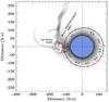 |
Fig. 1 To-scale sketch of the Vela X-1 system. HD 77581 is shown in blue and the orbit of the neutron star is represented by the black ellipse. Orbital phases are marked and labeled; phases covered in the present work are shown in red. We emphasize that the orbital phases are equidistant in time for the present orbital shape. We assume i = 73°, that is, lower limit for inclination according to Joss & Rappaport (1984), and the distances are thus lower limits. The background shows an indicative image of the variable large-scale structures that are formed through the interactions of the neutron star with the stellar wind of the mass donor. This image is an artistic impression based on simulations published in Manousakis (2011). The observer is towards minus infinity along the y-axis. |
We follow the standard Chandra threads and use CIAO 4.7 using CalDB 4.6.7, but employ a narrower sky mask to improve the flux at very short wavelengths by avoiding some of the overlap between extraction regions. For bright sources, such as X-ray binaries in general and Vela X-1 in particular, Chandra-HETG observations can be considered as essentially background-free. All analyses in this paper were performed with the Interactive Spectral Interpretation System (ISIS) 1.6.2 (Houck & Denicola 2000; Houck 2002; Noble & Nowak 2008). Uncertainties are given at the 90% confidence level for one parameter of interest.
2.1. Light curves and hardness
Figure 2 shows light curves extracted with the approximate time resolution of the neutron star spin period (283 s) in the 0.5–3 keV and 3–10 keV energy bands and the corresponding hardness, defined as the ratio between the harder and the softer band. We can distinguish two distinct behaviors: periods of highly variable high hardness and of stable low hardness. Interestingly, the total count rate changes by a factor of a few during the period of stable low hardness. Such increases in flux can be attributed to increases in the intrinsic X-ray brightness of the neutron star (e.g., Martínez-Núñez et al. 2014). To investigate the origin of the changing hardness, we time-filtered our observation and extracted one spectrum each for the low- and high-hardness periods using user-defined good time intervals corresponding to the two periods highlighted in Fig. 2. Exposures and total counts are listed in Table 1.
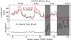 |
Fig. 2 Light curves and hardness ratio of Vela X-1 (Chandra ObsID 1928) in the 0.5–3 keV and 3–10 keV energy bands, binned to ~283 s. The hardness is defined as the quotient of the count rates in the 3–10 keV and 0.5–3 keV bands. Gray shaded areas indicate the time periods used to extract the high-hardness spectrum, and unshaded regions are used for the low-hardness spectrum. |
Exposure and total counts in hardness-resolved spectra.
2.2. Continuum variability
We first address changes in the overall continuum shape between low- and high-hardness periods. A physical model for X-ray continuum emission in accretion-powered X-ray pulsars is an open question (but see Becker & Wolff 2007; Farinelli et al. 2016; Wolff et al. 2016, for advanced approaches). Thus a multitude of empirical models, usually some combination of absorbed power laws, has been successfully used to describe spectra of accreting pulsars (e.g., Müller et al. 2013).
In Vela X-1, the presence of additional possibly X-ray emitting and reprocessing components such as the stellar wind, the denser material in the accretion, and ionization wakes, as well as the surface of HD 77851, make modeling the soft X-ray emission especially challenging (see Fig. 3 for an overview of the 0.8–9.5 keV spectrum). Below ~2.5 keV, the spectrum is complex and shows strong line features and peculiar continuum components such as a soft excess (Nagase et al. 1986; Hickox et al. 2004; Martínez-Núñez et al. 2014) that depend on orbital phase and absorption (Haberl & White 1990). We therefore define the continuum based on the 2.5–10 keV band, which does not include any strong lines with the exception of the Fe Kα complex (Torrejón et al. 2010; Giménez-García et al. 2015), which we exclude by ignoring the 6.2–6.5 keV band. To improve the signal-to-noise ratio (S/N), we combine the positive and negative first-order High Energy Grating (HEG) and Medium Energy Grating (MEG) data after rebinning to the MEG grid. We then rebin the combined spectrum to a S/N of 5 and a minimum of four MEG channels per bin.
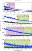 |
Fig. 3 Vela X-1 spectra from ObsID 1928 from low- (blue) and high-(black) hardness phases, HEG and MEG combined and rebinned by a factor of 2. Red dashed lines indicate the borders of the four regions (shaded) used in the local power law fits in Sect. 3. |
We describe the high- and low-hardness spectra each with a power law, defined by a power law index Γ and a normalization that is modified by absorption modeled with tbnew, the new version of tbabs (Wilms et al. 2000), using wilm abundances (Wilms et al. 2000) and vern cross-sections (Verner et al. 1996). The assumed model is simple and will not result in a perfect description of the continuum, but given the quality of the data it is adequate for our aim to assess continuum-shape changes.
To assess whether changes in absorption, expressed through the equivalent hydrogen column density, NH, or in power-law slope, Γ, lead to the hardness changes, we perform two fits, with results listed in Table 2. In a first fit, we assume that the absorption column, described by the NH parameter, is the same for both low and high hardness and tie this parameter between the two hardness modes. No acceptable fit can be obtained in this case. In a second approach, we assume the same power-law shape, that is, we tie Γ, but let the absorption be different. This model results in a better description of the data (Fig. 4).
Results of absorbed power law fits to the 2.5–10 keV continuum.
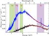 |
Fig. 4 Chandra-HETGSs spectra of Vela X-1 from ObsID 1928 from low-(blue) and high-(black)hardness periods. The best fitting absorbed power-law model with the same photon index, but varying normalization and absorption between the high- and low-hardness spectra, is shown in red in the modeled range. Shaded areas indicate the four regions used in the local power-law fits in Sect. 3. |
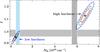 |
Fig. 5 Confidence intervals for independent power-law fits to low- and high-hardness data; crosses represent the best fit. The contours correspond to 1σ (red, dashed), 90% (green, dash-dotted) and 99% (blue, dash-dot-dotted) confidence intervals. The solid gray shaded region represents the values of Γ allowed when the power law slope is tied between the low- and high-hardness spectra; the light blue and gray patterned areas represent the corresponding allowed ranges for NH for low- and high-hardness spectra. |
Since there is still some systematic deviation between data and model above ~7 keV for the high-hardness spectrum, we also fit the two spectra with all model parameters independent of each other (Table 2). In Fig. 5, we show the confidence intervals for Γ and NH for this case as well as the 90% allowed ranges for Γ and NH for the case when the power law slope is tied between the two spectra. The confidence contours show the well known degeneracy between the derived values of Γ and NH (e.g., Suchy et al. 2008). We also see that letting Γ free leads to an even larger difference in hydrogen column density between the two spectra than when Γ is tied. The bulk of the changes in overall spectral shape are thus due to absorption and not due to changes in the shape of the underlying power law continuum, although some changes in spectral shape may also be present.
3. High-resolution spectroscopy
Having established that the changes in overall continuum shape between the low- and high-hardness periods are driven by changes in absorption, we now turn to high-resolution spectroscopy where we focus on regions below 2.5 keV (above 5 Å) as well as on the Fe Kα complex, which were not included in the broadband spectral modeling due to their complexity. We first visually inspect the differences between the low- and high-hardness spectra as presented in Fig. 3 and compare to the results of Goldstein et al. (2004) who analyzed the spectrum of ObsID 1928 without subdividing it into hardness-dependent periods. Because of the larger exposure and flux of the low-hardness data (Table 1), we expect that this period has dominated their analysis. We note a difference in line contributions between the spectra at different hardnesses: features change their relative strengths (e.g., lines of the He-like Si xiii triplet at ~6.7 Å, see Sect. 3.1), change from emission to absorption (e.g, Ne x Ly β at ~10.25 Å, see Sect. 3.3), and new features appear that were not found in the earlier analysis, such as lines from low-ionization stages of Si around ~7 Å (see Sect. 3.1).
In the remainder of this section, we model the low- and high-hardness spectra independently. As in Sect. 2.2, we combine the positive and negative first-order HEG and MEG data after rebinning to the MEG grid, but do not rebin the spectra further. Except where explicitly stated otherwise, we do not assume different line features to originate at the same location or the same medium, especially since multiple gas phases with different temperatures have been suggested as explanations for observations at higher orbital phases (Goldstein et al. 2004; Watanabe et al. 2006). Our analysis of the lines is based on local power-law continuum fits, that is, power-law continua describing a narrow interval around the respective features of interest. Although the slope, Γ, and normalization of such power laws do not have a direct physical meaning, we list the best fit results obtained for all regions discussed in the remainder of this section in order to facilitate reproducibility of results in Table 3. Our choice of wavelength intervals used for such local fits is informed by the previous knowledge of lines observed in Vela X-1 at other orbital phases (Schulz et al. 2002; Goldstein et al. 2004; Watanabe et al. 2006). We consistently use Cash statistics (Cash 1979) in this section as several of the considered intervals require it. We always first fit for the width of any component. However, since none of the detected Gaussian emission components are resolved at MEG resolution (0.023 Å FWHM), we fix their widths, σ, to σ = 0.003 Å, that is, about one third of the MEG resolution.
We use two approaches to search for lines: a blind search based on the Bayesian Blocks algorithm1 (Scargle et al. 2013) and a conventional, manual approach, where we utilize our knowledge of expected line energies of a given element. The Bayesian Blocks approach for spectral data is introduced, discussed, and benchmarked against other methods in Young et al. (2007). With this latter approach, we test for the existence of lines against a continuum model, starting with a power law that we iteratively fit to the data. At each iteration we extend the model by adding any lines found in the previous step.
The algorithm treats the data in an unbinned manner, but compares the changes in likelihood compared to the applied model2 for grouping the data into different numbers of “blocks”, with a single block corresponding to the absence of lines. For a given penalty factor, the algorithm exactly solves the 2n−1 problem, where n is the number of data bins, of how many blocks to divide the data into. A new block change point can start (or not) between any two bins, hence the 2n−1 possible divisions of the spectrum. A line is considered to exist between two such change points. Implementations of the Bayesian Blocks algorithm introduce a penalty factor that imposes a requirement for a minimum increase of the log likelihood to consider significance of the addition of a change point to the description of the function (e.g., spectrum or light curve). This penalty factor is controlled by an input parameter denoted by α in the work of Young et al. (2007) and by γ in notation of Scargle et al. (2013). The increase of the log likelihood is approximately equivalent to requiring that the addition of a change point exceeds a significance of p ~ exp(−α). Since a line requires two such change points, choosing an input of α = 1.5 is equivalent to requiring that lines have p< exp(−2α) ≈ 0.05, that is, they are at least 95% significant, or, P> 1−exp(−2α) ≈ 0.95.
Our analysis closely follows that of Young et al. (2007) where we start with a large value of α, apply the algorithm, and decrease α in steps of 0.1 until a line is found. We stop at a lower limit of α = 1.5. We list in Tables 4–8 the value of α at which (and below) the indicated line is found and call it αsig. The line significance is roughly interpretable as P ≈ 1−exp(−2αsig), but we note that, for example, He-like triplets are often detected as one excess encompassing all three lines.
3.1. Silicon region
We first address the silicon line region (6.0–7.4 Å). We point out that new laboratory reference data are available for the K-shell transitions of L-shell ions of Si, enabling robust velocity measurements (Hell et al. 2013, 2016).
3.1.1. High-hardness spectrum of the silicon region
The Bayesian Blocks approach finds three emission features, all with αsig> 3.3. We identify these lines with H-like Si xiv Lyα3, He-like Si xiii f forbidden line  –
– , also known as line z in the notation of Gabriel 1972) and a blend of the Kα lines from Si ii–Si iv. We model these features with Gaussians.
A visual inspection of the residuals, however, reveals further wave-shaped structures blueward of both Si xiii f and the Si ii–Si iv blend. We model these structures with one and two Gaussian lines, respectively, and identify them with the He-like Si xiii r resonance line ( –, also known as line w in the notation of Gabriel 1972) and blends of Kα transitions in N-like Si viii and O-like Si vii (Fig. 6).
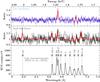 |
Fig. 6 Silicon region in the low- (upper panel, blue) and high-hardness (middle panel, black) spectra; both panels show combined HEG and MEG ± first order spectra normalized to their respective power-law continua. The solid red line shows the best model fits to the data. Residuals are shown in Fig. 7. The lower panel shows the calibrated and summed NASA/GSFC EBIT Calorimeter Spectrometer (ECS) silicon spectrum used for line identification. These data, as analyzed in Hell et al. (2016), are used as best currently available laboratory reference values for the energies of K-shell transitions in L-shell ions of Si. |
In our best fit model that uses six Gaussian emission lines, large-scale residuals that encompass the area around ~7 Å are still present. We model them with a broad Gaussian (σ ≈ 0.05 Å) in absorption that we explicitly do not interpret as a true line component but as complex continuum shape that a single power law fails to describe. The introduction of the broad Gaussian does not significantly change the obtained line positions. We note especially that the Bayesian Blocks approach relies on a good description of the continuum; the complex continuum shape therefore contributed to the failure of the automated approach to find the Si xiii r line and the Kα lines of Si vii and Si viii. We do not re-run the Bayesian Blocks algorithm on a continuum including the additional curvature that we modeled, as this would be inconsistent with a blind search.
Detected silicon emission lines.
Fitting just one Doppler shift for all detected Si lines does not result in a satisfactory model for the narrow features. In the interest of reducing free parameters, it is reasonable to assume that the lines with a similar ionization stage originate in the same medium. The lack of intermediate-ionization lines naturally leads to two line groups: (1) Si xiv Lyα, Si xiii f, and Si xiii r; and Si viii and Si vii Kα. We therefore fit one line shift to each of these groups (see Table 4 for reference values). Using this approach, we can obtain a good description of the data.
Although we formally fit a Doppler shift for the Si ii–vi Kα line blend, we do not take it into consideration when tying lines or discussing the overall behavior: the contribution of lines to a blend (and thus the measured center of the blend) depends on the properties of the plasma that are certainly different in laboratory and astrophysical environments (Hell et al. 2016). In fact, Hell et al. in their NASA/GSFC electron beam ion trap (EBIT) Calorimeter Spectrometer (ECS) data can distinguish two components in the Si ii–iv Kα lines, whose center they see at 1742.03 ± 0.06 eV: a blend of F-like Si vi Kα and Ne-like Si v Kα at  eV and a blend of Al- to Na-like Si ii–iv Kα at
  eV. Shifting the center of the full blend to 1740.04 eV would result in a change in measured velocity of >250 km s-1. A further complication is the possible presence of the Mg xii Lyβ at 7.106155 Å or 1744.74 eV (Erickson 1977).
The resulting properties of the Si lines are summarized in Table 4. The fits are shown in Fig. 6, where we show them in comparison with low-hardness data and lab measurements, and in Fig. 7, where we also show fit residuals.
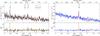 |
Fig. 7 Si-region spectra of high-hardness (left panel, black) and low-hardness (right panel, blue) periods. Lines identified in the spectra are indicated and labeled. Residuals to the best-fit model are shown in black/blue, and residuals to a power law without the narrow line components are shown in orange. Spectra normalized to their respective power-law continua and reference lab measurements are shown in Fig. 6. |
3.1.2. Low-hardness spectrum of the silicon region
In the low-hardness spectrum, we find one line with high significance (αsig> 8.5) at 6.73–6.75 Å and a complex w-shaped structure extending 6.98–7.05 Å at αsig = 1.5, that is, our lowest acceptable value of αsig, with the Bayesian Blocks approach.
We identify the Gaussian emission feature as Si xiii f line (Table 4). The w-structure can be empirically described as a combination of emission and absorption lines at the same energy. This results in lines with widths σem ≈ σabs ≈ 0.013 ± 0.002 Å at a wavelength of 7.022 ± 0.003 Å and precludes a line identification (Figs. 6 and 7): if this were the Si vii Kα line blend, it would have a Doppler velocity of ~−1500 km s-1, comparable to the one measured in the high-hardness spectrum. However, no other silicon lines except Si xiii f are present in the low-hardness spectrum and it would require extreme fine-tuning to produce the Si vii Kα line alone. The peculiar shape of the feature also remains a problem. Regarding other elements, while the Rydberg series of He-like Mg xi, H-like Mg xii and H-like Al xiii have some Kα transitions surrounding this region, none of them is sufficiently close or strong enough to explain this feature. Both H-like Mg xii Lyβ at 7.10616 Å and H-like Al xiii Lyα at 7.17272 Å (Erickson 1977) are too high in wavelength. While the He-like Mg xi series has several n ≥ 7 → 1 transitions between 7.174 Å (n = 7; Verner et al. 1996) and 7.037 Å (series limit or ionization potential; Drake 1988) there is no indication from lines earlier in the series that the lines should be strong enough to explain the observed feature. Still, a radiative recombination continuum (RRC) feature of Mg xi at 7.037 Å (Drake 1988) could contribute to the observed feature.
3.2. Magnesium region
We next address the 8.0–10 Å region, that is, from longwards in wavelength of Mg xii Lyα to shortwards of the Mg iv Kα blend. Several 4 → 2 transitions from Fe xxi to Fe xxiv fall into this region, but their location noes not agree with any of the features detected in the following, and we do not detect any of the corresponding stronger 3 → 2 transitions from Fe xxi to Fe xxiv (Brown et al. 2002) in Sect. 3.3.
3.2.1. High-hardness spectrum of the magnesium region
We identify the first line found (αsig = 5.4) by the Bayesian Blocks approach with Mg xii Lyα (8.42101 ± 4.0 × 10⁻⁵ Å, Erickson 1977). The algorithm further finds a very shallow step in the residuals at ~9.5 Å, consistent with the location of the magnesium K edge. However, the step implies an excess where, from an edge, we would expect additional absorption and, consistently, the inclusion of an edge does not improve our model. Indeed, the best-fit optical depth of the edge component is zero, that is, no edge is present, therefore we do not use this component further.
The next detected component consists of a broad excess spanning the whole He-like Mg xi triplet (r: –; i:  – and
– and  –, also known as lines x and y in the notation of Gabriel 1972; f:
  –) and with a stronger narrower excess at the Mg xi forbidden line. We include all three He-line triplet lines in our model, tying the distance between the triplet lines and the Lyα line to reference values from Drake (1988, for He-like) and Erickson (1977, for H-like). The last feature detected with the Bayesian Blocks approach is an emission feature at ~8.95 Å (αsig = 2) that we cannot identify with an obvious line of magnesium or iron (Figs. 8, lower panel, and 9, left panel).
Magnesium emission lines in the low- and high-hardness spectra.
We parametrize the line strengths of the He-like triplet using the ratios R = f/i and G = (f + i) /r (Gabriel & Jordan 1969; Porquet & Dubau 2000) and model these density and temperature diagnostics directly. We obtain R = 1.5 ± 0.7 and  and a line shift of −140 ± 80 km s-1 for the identified H- and He-like Mg lines (see Table 5 for detailed line parameters of the identified lines).
It has been recently shown by Mehdipour et al. (2015) that, under astrophysical conditions, He-like triplet lines of a given element can be affected by absorption from Li-like ions in the same medium. While Mehdipour et al. (2015) discuss this effect for the cases of iron and oxygen, it can easily be extended to other elements. Contamination of the He-like magnesium triplet in emission by absorption lines is clearly seen in the following only for the low-hardness spectrum (Sect. 3.2.2). While we do not detect any absorption lines in the high-hardness spectrum, we cannot exclude some contamination of the triplet.
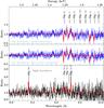 |
Fig. 8 Magnesium region in low (blue, upper two panels) and high (black, lower panel) spectra, corresponding to high and low absorption, respectively. The panels show combined HEG and MEG ±1 order spectra normalized to their respective power-law continua. The solid red line shows the best model fit to the data. Two models for the high-absorption data are shown that differ in their treatment of absorption lines: five individual lines with independent Doppler shifts (upper panel) and a template consisting of Mg xi to iv Kα, all with the same Doppler shift (lower panels). We further show the reference positions of Mg xi to iv Kα (Behar & Netzer 2002) as well as for the H-like Mg xii Lyα and He-like Mg xi triplet lines. |
3.2.2. Low-hardness spectrum of the magnesium region
The Bayesian Blocks approach finds discrete absorption features at ~9.15 Å (αsig> 7), ~9.29 Å (αsig> 4.6), ~9.7 Å and ~9.8 Å (αsig = 2.0). It also finds a wide excess at ~9.1–9.3 Å, consistent with the location of the Mg xi triplet that becomes more pronounced as the narrow absorption features are iteratively taken into account by the model. We model the He-like triplet as in the case of the high absorption spectrum by fixing the relative location of the lines but leaving one line energy and the strengths of the individual lines free. The last component is a discrete absorption feature at ~9.77 Å (αsig = 2.4).
The resulting model includes eight lines: the He-like triplet lines in emission and five absorption lines (Figs. 8, upper panels, and 9, right upper panel). In spite of suggestive residuals, no significant Mg xii Lyα is found and we leave it out in our best-fit model.
Since the absorption lines are weak and their widths unresolved, we are able to replace the narrow Gaussian absorption components used so far with a simple multiplicative box-function4 and thus fit their equivalent widths directly. For the emission lines of the He-like triplet we obtain velocities of −130 ± 60 km s-1 (He-like triplet line parameters in Table 5).
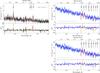 |
Fig. 9 Mg-region spectra of high-hardness (left panel, black) and low-hardness (right panels, blue) periods. Residuals to best fit model are shown in black/blue, residuals to a power law without the line components in orange. The upper right panel shows a fit with five independent absorption lines. The lower right panel shows a fit using a template for Mg-series from Mg xi to iv (reference energies according to Behar & Netzer 2002, indicated by solid lines) with one Doppler shift for all lines. Spectra normalized to their respective power-law continua are shown in Fig. 8. For the high-hardness region, lines identified are indicated and labeled. For the low-hardness region, we refer to the Tables 5 and 6 for the identified lines. |
Magnesium absorption lines in the low-hardness spectrum.
The locations of the absorption lines are indicative of the different ionization stages of Mg. We use the theoretical reference values for the line energies of He-like Mg xi r to F-like Mg iv Kα lines from Behar & Netzer (2002) to identify the lines (Fig. 8) and calculate the line velocities (Table 6).
The Ne x Lyγ line at 9.70818 Å (Erickson 1977) is very close to N-like Mg vi Kα at 9.718 Å and indeed, Goldstein et al. (2004) have identified this absorption feature with Ne x Lyγ. While we detect Ne x Lyβ (Sect. 3.3.2), this line is blue-shifted by  km s-1; a Ne x Lyγ line with a similar shift does not describe the observed absorption feature. We also do not detect the neighboring Ne x Lyδ at 9.48075 Å (Erickson 1977), although our upper limit on the equivalent width of this line is −4 × 10⁻³ Å, that is, within the margins of our expectations of the strength of Ne x Lyδ given the equivalent width of Ne x Lyβ. On the other hand, assuming, as done here, that the two prominent absorption features at 9.7–9.8 Å are from Kα transitions in N-like Mg vi and O-like Mg v results in similar strengths for both lines, which both appear blue-shifted, consistent with the detected higher ionization Mg ions, confirming our line identification. We cannot, however, exclude a contribution of Ne x Lyγ to the observed feature we identify as Mg vi Kα in absorption. To test the amount of this contribution, we model the observed absorption feature with two components, one of them at the expected location of blue-shifted Ne x Lyγ. We obtain similar velocity and equivalent width for Mg vi Kα as without the neon contribution (v = −280 ± 90 km s-1 and
  Å) and an equivalent width of
  Å for Ne x Lyγ.
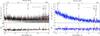 |
Fig. 10 Neon region spectra. Left panel (black): high-hardness spectrum. Right panel (blue): low-hardness spectrum. Best-fit models shown in red. Residuals of the Cash statistics for best fit including the lines shown in black and blue, respectively; residuals to the power law only in orange. The identified lines are indicated and labeled. |
The obtained velocity values for the absorption lines of Mg span a wide range of −(300–900) km s-1 (Table 6) and are inconsistent with each other within their uncertainties. However, the complexity of the spectrum, in particular the overlap of emission and absorption features can lead to modeling problems that the formal errors do not account for. Additionally, inaccuracies in theoretical reference values may be present: while no EBIT laboratory data are yet available for magnesium, Hell et al. (2016) have shown that for silicon and sulfur, laboratory values and theoretical calculations of Behar & Netzer (2002) can disagree at up to 300 km s-1, especially for lower ionization stages.
To better assess the contributions of the Mg absorption lines, we build a template (Mg xi to Mg iv Kα, Fig. 8 and Table 6) using the Behar & Netzer (2002) values: we assume the same line shift for all lines, but let the line strengths vary. For B-like Mg viii and C-like Mg vii, Behar & Netzer (2002) list two strong transitions. For each ion, both transitions are of comparable oscillator strength but are, respectively, 0.016 Å and 0.024 Å apart, which corresponds to a velocity difference of ~500 km s-1 and ~750 km s-1, respectively (cf. Fig. 8 where the line positions are marked). We incorporate these lines in our template using one line with the average line center as listed in Table 6, but note that this can lead to additional uncertainties in the determination of the line Doppler shifts. We also include the He-like Mg xi triplet in emission with parameters as described above and show the resulting best-fit model in Figs. 8, middle panel, and 9, lower-right panel. The line template parameters are listed in Table 6. The template line velocity of −360 ± 40 km s-1 is in rough agreement with the average velocity of the five independent absorption lines. The equivalent widths of the template lines show that B-like Mg viii and F-like Mg iv Kα are consistent with 0, that is, the lines are not significantly detected, consistent with their non-detection in the Bayesian Blocks approach. The equivalent width of C-like Mg vii Kα may indicate a weak line. The large uncertainties on Li-like Mg x Kα, on the other hand, are due to the blending of the line with the intercombination and forbidden emission lines of the He-like Mg xi triplet.
3.3. Neon region
The region of interest encompasses the wavelengths 10–14 Å, that is, from H-like Ne x Lyβ to the He-like Ne ix triplet. At higher wavelengths, low source counts preclude an analysis and in particular the detection of possible Kα features of lower ionization stages than Ne viii. All identified neon lines in both low- and high-hardness spectra are listed in Table 7 together with their respective reference values.
3.3.1. High-hardness spectrum of the neon region
The Bayesian Blocks approach finds H-like Ne x Lyα with αsig = 3.4, an excess spanning the location of the He-like Ne ix triplet with αsig = 2.5, and finally the H-like Ne x Lyβ with αsig = 2. No further structure is detected with this approach once these five lines are included.
We fit just one line shift for all five lines. Similarly to Sect. 3.2.1, we directly fit the He-like triplet line ratios, R and G (e.g., Porquet & Dubau 2000) and obtain  and
and  . The resulting line velocity is −220 ± 70 km s-1 (Fig. 10).
Neon lines in the low- and high-hardness spectra.
3.3.2. Low-hardness spectrum of the neon region
The Bayesian Blocks approach finds a complex feature that we identify with the He-like Ne ix triplet lines (αsig = 5) and model with Gaussian components. The feature shows a dip between the Ne ix f and Ne ix i component and we model it with a narrowline component that we identify with the Li-like Ne viii Kα. The next strongest feature is H-like Ne x at αsig = 4.6 that we fit with a Gaussian. We also note that the strong Fe xvii  –
– transition (commonly denoted as 4C) is located at 12.124 Å (Brown et al. 1998), that is, close to H-like Ne x, but we do not detect any other strong lines from iron, making an identification of the observed absorption feature with this line doubtful.
The presence of the Ne viii Kα line hints towards a complex interplay of absorption and emission features as also already seen in the low-hardness spectrum of the magnesium region (Sect. 3.2.2).
We tie the centers of the four emission features together and obtain a line velocity of  km s-1. For Ne viii Kα, we obtain v = −220 ± 140 km s-1, but given the low counts in the spectrum and the interplay of the emission and absorption, the formal errors are likely underestimated.
Because of the presence of H-like Ne x Lyβ in the low-hardness spectrum and suggestive residuals at ~10.2 Å, we add this line in absorption to our model and obtain an equivalent width of  Å and a line velocity of km s-1. This velocity is inconsistent with that of the emission lines and attempts to tie the velocities do not result in a satisfactory fit. The presence of Ne x Lyβ does not change the modeling results for other lines in the region.
For a single uniform medium, lines of the same series are expected to be all either in absorption or in emission. However, in the case of Vela X-1 we expect a complex geometry, as discussed in Sect. 4, and the sum of emission and absorption line contributions from different regions could result in the observed properties of the Ne x Ly series. The overall behavior however remains puzzling.
3.4. Iron Kα region
The region encompasses wavelengths in the range 1.6–2.5 Å, that is, the locations of the neutral Fe Kα (1.937 Å) and Fe Kβ (1.757 Å) lines as well as the iron edge (1.740 Å) and Ni Kα (1.66 Å) line. The use of a broader region than covered by the line features themselves allows better constraints on the power-law continuum. The results for this section are listed in Table 8 and shown in Fig. 11.
In the high-hardness spectrum, the Bayesian Blocks approach first finds the obviously present Fe Kα line, followed by the Fe Kβ and a step-like feature that we identify as the iron edge. We model the lines with Gaussian components and the edge with the edge model, fixing the edge energy to 1.740 Å (Fig. 11). The resulting line and edge parameters are listed in Table 8. Ni Kα has been previously detected in Vela X-1 (e.g., Martínez-Núñez et al. 2014). However, no feature at the location of the Ni Kα shortwards in wavelength from the edge is found with Bayesian Blocks; there is a strong nearby residual in the low-hardness spectrum, but given the low counts and large uncertainties of this region and the fact that the feature is only one bin wide, we do not consider it to be a physical Ni Kα line.
Emission lines and absorption edge in the iron Kα region.
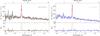 |
Fig. 11 Fe region spectra. Left panel: high-hardness spectrum. Right panel: low-hardness spectrum. Data are shown in upper panels in black and blue, best-fit model in red. Residuals of best fit including the lines and edge (high-hardness spectrum) are shown in black and blue, respectively; residuals for the power law only are shown in orange. |
In the low-hardness spectrum, the Bayesian Blocks approach finds only the Fe Kα and Fe Kβ lines. The inclusion of the edge, however, still improves the fit and we obtain an absorption edge depth of 0.05 ± 0.04, that is, marginally inconsistent with zero.
4. Discussion
4.1. The source of varying absorption column density
Past analyses have established a relatively stable behavior of the central X-ray engine in Vela X-1 (Odaka et al. 2013) even during major flares (Martínez-Núñez et al. 2014). Our modeling in Sect. 2.2 suggests that the rapidly changing absorption is at least one of the sources of the observed changes of spectral shape but we cannot exclude changes in the underlying spectral shape as a further contribution. Physical origin of possible changes in spectral slope has been discussed, for example, by Odaka et al. (2014). Inhomogeneous absorption by clumpy matter has been used in Vela X-1 by Nagase et al. (1986) to explain the transient soft excess. Such absorption changes are expected either if the wind that the neutron star is accreting from is clumpy (review by Martínez-Núñez et al. 2017, and reference therein) or if the inner parts of the accretion flow are highly structured (Manousakis 2011; Manousakis & Walter 2015); both effects could be present simultaneously.
Clumpy winds are expected for O/B stars: line-driven winds of such stars are subject to instabilities (Lucy & Solomon 1970; Lucy & White 1980). Hydrodynamical simulations show that perturbations are present, grow rapidly and cause strong shocks so that dense gas-shells form (Owocki et al. 1988; Feldmeier et al. 1997). Density, velocity, or temperature variations compress the gas further and fragment it into small, overdense clumps embedded in tenuous hot gas (e.g., Oskinova et al. 2012; Sundqvist & Owocki 2013). In the HMXB Cyg X-1, for example, the clumpy wind paradigm has been used to explain the absorption dips, long-term variability of the absorption along the orbit, and the changing line content observed in high-resolution spectra during dips (Hanke et al. 2009; Grinberg et al. 2015; Miškovičová et al. 2016). In Vela X-1, clumpy winds can reconcile the discrepancies between different estimates of the mass-loss rate (Sako et al. 1999). Several lines of evidence also point towards the presence of wind clumping very close to the photosphere of O/B stars (Cohen et al. 2011; Sundqvist & Owocki 2013; Torrejón et al. 2015), well within the ~1.7 RHD 77581 distance between the neutron star and HD 77581 in Vela X-1.
To evaluate the impact of the clumpiness along the line-of-sight on the time variability of the column density, we designed a toy model consisting of a point source with a constant X-ray flux orbiting an O/B star at an orbital separation of 1.8 R⋆ (Fig. 12). The wind is represented relying on the multi-dimensional numerical simulations of Sundqvist et al. (2017). They computed, as a function of time, the mass-density, velocity and pressure profiles in the wind up to 2 stellar radii. Doing so, they witnessed the formation of small overdense regions (clumps), embedded in a lower-density environment, and determined their dimensions and mass. We assumed an edge-on inclination and a self-similar expansion of their results to extend their simulation space to up to 15 R⋆ and computed the column density along the line of sight at φorb = 0.21–0.25. Beyond the expected systematic decrease in column density as the compact object moves towards us, we observe a 30% peak-to-peak spread with a correlation time of at most 1 ks, a few times longer than the self-crossing time of the clumps. The combined absorption of independent clumps along the line-of-sight thus leads to larger and longer increases in column density than a single clump passing by, but not by a factor of a few in amplitude and not for a few kiloseconds. Therefore, given the characteristic size, speed, and distribution of clumps in the wind of isolated massive stars (Sundqvist et al. 2017), the inhomogeneities in a wind unperturbed by the presence of the compact object are not enough to account for the observed enhanced absorption (Sect. 2.2).
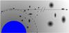 |
Fig. 12 Illustration (not to scale) of the computation in Sect. 4.1. The inhomogeneous wind induces a time-variable column density on the line of sight (solid line) as the constant X-ray flux point source (cross) orbits the star (in blue) at φorb = 0.21–0.25 (arc interval). The overdense regions are fiducially represented using radially fading spheroidal black dots and the inter-clump environment using a smoothly decaying spherical profile. |
However, the compact object can significantly alter the wind structure, either through its gravitational (El Mellah & Casse 2017) or its radiative influence (Blondin et al. 1990; Manousakis & Walter 2015). The emerging structures (tidal stream, trailing accretion and photoionization wake) highly modulate the systematic orbital evolution of the column density (observational evidence in, e.g., Kaper et al. 1994; Fürst et al. 2010; Doroshenko et al. 2013; Malacaria et al. 2016). Yet, their influence should be minimal around φorb ≈ 0.25 since most of the aforementioned orbital-scale structures lie essentially along the axis joining the two body (star and neutron star) centers or trail the neutron star (Fig. 1). In this way, they are far enough from the line of sight that we do not expect much of the variation in the column density to be associated to them. Still, closer to the neutron star, Manousakis & Walter (2015) showed that even assuming a smooth upstream wind, the flow is highly structured and variable within the shocked region, possibly giving rise to changing absorption such as that observed here. Further numerical investigations are ongoing and aim at following the clumps as they encounter the shock (El Mellah et al. 2017): the role the clumps play in time-varying absorption would be altered by the deceleration and compression they undergo at the shock. There is also observational support for the presence of such shocks in Vela X-1 since its broadband X-ray count rate has been shown to follow a log-normal distribution (Fürst et al. 2010). This distribution can be described by a multiplicative stochastic model (Uttley et al. 2005; Fürst et al. 2010) and is known to be a possible result of shocks acting on clumpy material (see, e.g., Kevlahan & Pudritz 2009).
Further, newest calculations for stellar-atmosphere models estimate the wind velocity in the inner region, where the neutron star is located, to be as low as ~ 100 km s-1 (Sander et al. 2017b), that is, on the order of the orbital velocity. In such a case, the wind and accretion structure could be significantly altered (Shapiro & Lightman 1976), possibly leading to the formation of a transient disk whose formation and dissipation could, for example, result in absorption and flaring events. A detailed modeling of such an accretion flow is beyond the scope of this paper, but we point out that, to the knowledge of the authors, no clear disk signatures have yet been detected in any of the X-ray observations of Vela X-1.
4.2. He-like triplet diagnostics: properties of the X-ray emitting gas
We measured the ratios R = f/i and G = (f + i) /r (Gabriel & Jordan 1969; Blumenthal et al. 1972; Porquet & Dubau 2000) for the He-like Mg xi and Ne ix triplets in the high-hardness spectra and obtain R = 1.5 ± 0.7 and (Sect. 3.2.1) and and (Sect. 3.3.1), respectively. The presence of strong resonance lines (Figs. 8 and 10) and the measured best fit value of G< 4 for magnesium imply that the He-like triplets in the high-hardness spectrum may not be consistent with emission from a purely recombination-dominated photoionized plasma. While we do not use the Si xiii triplet to calculate G and R, the two measured lines in the high-hardness spectrum, Si xiii r and Si xiii f, are of comparable strengths, while the intercombination line is too weak to be detected (Figs. 6 and 7 and Table 4), supporting the results obtained for Mg and Ne. We do, however, emphasize the large uncertainties of the R and G values we obtain from our fits: the following discussion of plasma diagnostics should thus be seen as a roadmap for future investigations with missions with a larger collecting area such as JAXA’s X-ray Astronomy Recovery Mission (XARM) or ESA’s Athena (Nandra et al. 2013).
In principle, G< 4 (but note that G = 4 is still within the large measured uncertainties) could be due to the presence of a collisionally ionized component, which is predicted to have a much lower G ratio of ~1. However, it has been shown in a number of other accretion-powered photoionized plasmas that resonance scattering can also contribute to the emission, with the relative contributions of resonance scattering and recombination determining the observed G ratio (Sako et al. 2000; Kinkhabwala et al. 2002, 2003; Wojdowski et al. 2003). Kinkhabwala et al. (2002) calculated spectra for different ionic column densities in the ionization cone of a Type 2 Seyfert galaxy (i.e., viewed from the side, with direct emission from the central source obscured); based on Fig. 7 of their article, we can estimate that an ionic column density of order 1018 cm2 is consistent with the observed G ratios of Ne ix and Mg xi.
To estimate the elemental column densities in the wind, we first calculate the characteristic hydrogen column density of the wind, N⋆, that is defined as (1)with Ṁ being the mass-loss rate, μ the mean weight, mp the proton mass, R⋆ the radius of the star and v∞ the terminal velocity of the wind. This is the hydrogen column density that would be observed along a line of sight from the observer to the stellar surface in the case of constant wind velocity, and is a good order-of-magnitude proxy for the typical column density experienced by X-rays escaping along different lines of sight from the neutron star. For the typical values for HDE 77581, that is, Ṁ ~ 2 × 10⁻⁶M⊙ yr-1, v∞ = 750 km s-1, and R⋆ = 30 R⊙, we obtain N⋆ = 2.4 × 1022 cm-2. Using the abundances of Wilms et al. (2000), we then estimate typical elemental column densities of 2 × 10¹⁸ for Ne ix, 6 × 10¹⁷ for Mg xi, and 4.5 × 10¹⁷ for Si xiii. These crude estimates for the elemental column densities are of order comparable to the above estimate of the ionic column densities from the G ratios, implying that a substantial fraction of the material along the line of sight is ionized to the He-like charge state for each of these elements. Further, more stringent observational constrains on G ratio at φorb ≈ 0.25 will be crucial to confirm or refute this line of argumentation that can currently be cast in doubt by the large measured uncertainties on G.
The measured values of R are not consistent with expectations for a low-density photoionized plasma. This is particularly striking for neon, where we would expect R ≈ 3.1 for a low-density plasma with T = 2 × 10⁵ K and higher R for higher temperatures (Porquet & Dubau 2000), all values above the measured . One possible interpretation is that the plasma density is high; however, the implied densities of 1012–1013 cm-3 (Porquet & Dubau 2000, Fig. 9) are much higher than expected anywhere in the wind, or even in the accretion wake, and should only be found in the hydrostatic part of the stellar atmosphere. Possible structures close to the neutron star such as discussed in Sect. 4.1 are unlikely to lead to such extreme density enhancements; typical high densities reached in the simulations of Manousakis (2011) or Mauche et al. (2008) are of the order of a few 1010 cm-3 and below. On the other hand, it is well known from studies of single OB stars (Kahn et al. 2001) that the strong stellar UV field of HDE 77581 will reduce the forbidden line strength near the star by depopulating the metastable level (Gabriel & Jordan 1969; Blumenthal et al. 1972; Mewe & Schrijver 1978; Porquet et al. 2001).
In Fig. 13, we show predictions for the R ratio as a function of stellar radius for a B-type star with stellar parameters similar to HDE 77581 (Teff = 25 000 K, log g = 3.0), using a methodology similar to that described in Sect. 2 of Leutenegger et al. (2006) to average over the relevant part of the TLUSTY model stellar continuum, that is, a non-LTE, plane-parallel, hydrostatic model stellar atmosphere (Lanz & Hubeny 2007), to estimate the UV field. In the context of the predicted ratios, and assuming a single radius of formation, the measurements would imply a formation radius of at least a few stellar radii, thus ruling out a substantial contribution of emission from the undisturbed stellar wind near the neutron star at r ≈ 1.7 RHD 77581 for Ne ix and Mg xi.
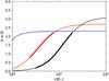 |
Fig. 13 Predicted R = f/i ratio as a function of radius (expressed in multiples of stellar radius) for Ne ix (black), Mg xi (red), and Si xiii (blue) for a B star with similar parameters to HDE 77581. The thickened portions of the Ne ix and Mg xi curves show the 90% confidence interval for measured values of R and thus for the radius. |
4.3. Presence of multi-component medium
In eclipse (φorb ≈ 0), co-existing emission lines from high- and low- ionization species of several elements have previously been detected by Sako et al. (1999) and Schulz et al. (2002) and in both cases interpreted as signatures of a multiphase medium, with cool dense clumps co-existing with hotter plasma. Similarly, the simultaneous presence of emission lines from high- and low-ionized ions of the same element at orbital phase 0.5, when the source is strongly absorbed by the accretion wake (Fig. 1), implies multiple gas phases with different temperatures in the medium (Goldstein et al. 2004; Watanabe et al. 2006).
Here, at φorb ≈ 0.25, we detect Kα transitions of L-shell ions of both silicon in emission in the high-hardness spectrum, that is, at higher overall absorption (Sect. 3.1.1), and of magnesium in absorption in the low-hardness spectrum, that is, at lower overall absorption (Sect. 3.2.2). In both cases, the L-shell ions co-exist with H- and He-like ions from the same elements. In the case of magnesium, we detect absorption from Mg xi r and Kα lines from Li-like Mg x, Be-like Mg ix, N-like Mg vi, O-like Mg v and, tentatively, C-like Mg vii. These lines imply the presence of cooler material in the system outside of the large-scale accretion structure, which should not be crossing our line of sight at φorb ≈ 0.25 (Fig. 1), as the comparatively modest measured absorption also implies. Clumps in the structured wind would provide a natural explanation for such material but so would a structured flow close to the neutron star. While detailed theoretical considerations of the interaction of a clumpy wind with a compact object and its radiation are beyond the scope of this work, we undertake two simplified estimates of whether or not the observed signatures can be produced in a single-zone absorber assuming a photoionized wind (Sect. 4.3.1) and whether or not the observed L-shell transitions may come from ions present in the stellar wind itself (Sect. 4.3.2).
Further hints of the presence of multiple components come from the detection of Ne x Lyβ in absorption and Ne x Lyα in emission in the low-hardness and thus low-absorption spectrum (Sect. 3.3.2). Lines of the same element in both emission and absorption cannot be produced in a single uniform medium and the observation can only be explained through the presence of multiple components whose sum results in the observed spectrum. Both, Ne x Lyα and Lyβ are detected in emission in the high-hardness and thus high-absorption spectrum (Sect. 3.3.1).
4.3.1. Photoionization simulations
First, to simulate a photoionized wind medium, we approximate the broadband spectrum of the irradiating continuum as the sum of the emission from the neutron star and from the companion. Since our data do not extend above 10 keV, we rely on the broadband (~3–70 keV) fits to NuSTAR observations obtained by Fürst et al. (2014) for the description of the neutron star continuum. They analyze two observations and find that a power-law model with a Fermi-Dirac cut-off (FDCUT; Tanaka 1986) gives a good description of the data:  (2)where A is the overall normalization, Γ the photon index, Ecut the cut-off energy , and Efold the folding energy. We use Γ = 0.99, consistent with our measurement in Sect. 2.2 and with the average Γ obtained by Fürst et al. (2014) for their two observations, and set the normalization to 0.277 keV-1 cm-2 s-1 (at 1 keV), the value we measure. Using their average values, we also set Ecut = 20.8 keV and Efold = 11.9 keV. We model the contribution of HD 77581, which dominates the UV-continuum, as a blackbody using the parameters from Nagase et al. (1986): distance of 2 kpc, stellar radius of 31 R⊙ and temperature of 25 000 K.
For our purposes here, it is sufficient to determine whether or not we can produce the observed range of Kα absorption lines of magnesium ions, from Mg v to Mg xi, in a single-zone absorber. With the above continuum model, we use XSTAR v2.315 to calculate the ionization balance in the illuminated material for three different densities: 104,1010, and 1016 cm-3. Using line optical depths from XSTAR, we then generate approximate synthetic spectra from 8 to 10 Å, at the ionization parameters6ξ1, where Mg v and Mg xi have comparable ion fractions, and ξ2, where Mg v peaks. Regardless of density, at ξ1 we overpredict the strength of the Mg xii line at 8.42 Å, and significantly underpredict the Mg v line. In general, at both ξ1 and ξ2, we expect lines from Mg vi to Mg viii that are comparable to or stronger than our Mg v/Mg xi lines of interest.
In short, it is difficult to produce both Mg v and Mg xi in a single absorption zone without producing other strong Mg lines between 8 and 10 Å. While such lines are not negligible in our data, they are generally weaker than we would expect based on our XSTAR calculations; further XSTAR runs show that the discrepancy between predictions and observations is exacerbated if we suppose that the absorber is shielded from the stellar continuum and only illuminated by the neutron star. Thus, although we have not performed any detailed ionization modeling of the absorber, it is unlikely that the observed lines originate in a single ionization zone. For the continuum spectra and ionization parameters considered here, the gas appears to be thermally stable (Krolik et al. 1981), indicating that multiple distinct absorbers (rather than a multi-phase gas) may be required.
4.3.2. Stellar atmosphere modeling
In a second approach, we use a detailed wind model for the donor star to see which ions are to be expected and how this changes due to the presence of a strong X-ray source. We employ the hydrodynamically consistent stellar atmosphere model calculated for Vela X-1 (Sander et al. 2017b) using the most recent version of the Potsdam Wolf-Rayet (PoWR) model atmosphere code that is able to obtain the mass-loss rate and wind stratification self-consistently for a given set of stellar parameters (Sander et al. 2017a). This model takes into account density inhomogeneities in the wind in the form of optically thin clumps but does not include changes in the wind geometry due to the presence of the neutron star.
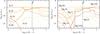 |
Fig. 14 Relative population numbers for the ground states of silicon (left) and magnesium (right) vs. the distance from the donor star in two hydrodynamically consistent PoWR models describing the wind of HD 77581. The dotted lines refer to a model without X-ray illumination, while the simple lines denote the ionization stratification for a model with an X-ray illumination comparable to the situation in Vela X-1; same color represents the same ionization stage of an element. The vertical line denoted with dns marks the location of the neutron star. |
For the purpose of our work, the donor star models from Sander et al. (2017b) were recalculated to account for higher Mg ions up to Mg viii and we refer the reader to this work for the details of the calculations. In these models, Si is covered up to Si vi. While we do see higher ions in our X-ray observations, they would not be expected from a single massive star wind (Fig. 14, blue curves). For the model without X-rays, only lower ions of both elements are found. For silicon, Si iv is leading in the wind until Si iii takes over in the outer part. Close to the donor star, Si v also plays a role, but already Si vi is essentially not populated in the wind. For magnesium, the situation is even simpler with Mg iii being the leading ion in the wind and all higher ions quickly becoming depopulated beyond the surface of the donor.
The situation changes when X-rays are included. Although the treatment of the X-ray irraditaion in the atmosphere models is only a rough approximation, as these are 1D models and the X-rays are modeled as Bremsstrahlung, the changes in the population numbers illustrate that the X-ray illumination due to the accretion onto the neutron star leads to a more complex structure and to the presence of several higher ions. Si vi and Si v are now only about an order of magnitude less populated than the leading Si iv; they remain important until the wind is essentially transparent and Si vi becomes the leading ion in the outer wind (Fig. 14, left panel). For magnesium, the situation is roughly similar, but more complex as more ions are present (Fig. 14, right panel). At the distance of the neutron star, the previously unimportant ions Mg iv to Mg vii are now almost similarly populated. At larger distances, Mg vii becomes the leading ion and only Mg vi remains significantly populated. Interestingly, the relative population of Mg viii increases outwards, but then drops down again. However, the later could be an artifact from our restriction to 1D models with monotonic wind velocity laws.
In spite of the limitations of our models, we can conclude that the ionization situation around Vela X-1 is complex. The PoWR models have demonstrated that the donor wind as such produces very low ionized metals (e.g., C iii, Mg iii, Si iv, Fe iv), but the illumination due to X-rays changes this situation significantly and even in the 1D approach, distinct regions with different leading ions are present. However, the model also demonstrated that some ionization stages can exist in the same region. Given the fact that due to the orbit of the neutron star only a part of the wind is strongly illuminated, while other parts are less or even not at all affected by X-rays, it is safe to conclude the observed X-ray spectrum stems from a multitude of layers with different ionization situations.
4.4. Iron fluorescence
The location of the detected Fe Kα emission features (Table 8) is consistent with the Kα1 and Kα2 lines of neutral or lowly ionized iron ions below Fe xii (House 1969). Interestingly, PoWR model atmosphere calculations for Vela X-1 (Sander et al. 2017b, see also Sect. 4.3.2) imply that the main iron ion species present in the wind without X-ray irradiation should be Fe iv, followed by Fe iii. In the case of strong X-ray irradiation, Fe v becomes more strongly populated and surpasses Fe iii. Furthermore, in this case, higher ionization stages (Fe vii and above) can also be reached in the outer wind.
The flux ratio between Fe Kβ and Fe Kα is consistent with the theoretical expectations of ~0.13–0.14 (Palmeri et al. 2003). We note, however, the large uncertainties on Fe Kβ which are exacerbated by the presence of the Fe K edge.
Kallman et al. (2004) predict the curve of growth for the equivalent width of Fe Kα, EQW(Fe Kα), in units of eV, and the hydrogen equivalent absorption column density of the reprocessing material,  , in units of 1022 cm-2, to be
 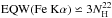 (see also Inoue 1985). This has been observationally verified for HMXBs by Torrejón et al. (2010) using a Chandra-HETG sample that included Vela X-1. To compare our results, we calculate the equivalent width of the Fe Kα and Kβ lines in eV (Table 8) and use the values for NH obtained from continuum fits (Sect. 2.2). The observed lines are much stronger than would be predicted by the above correlation; however, Torrejón et al. (2010) obtain similar results for the same data: in their analysis, Vela X-1 clearly lies above the correlation.
Several effects can contribute to the disagreement between the measured values and the theoretically predicted curve of growth: on one hand, NH measurements are generally dependent on the continuum model and our choice of a power law to describe the 2.5–10 keV may lead to systematic deviations, although we note that our results roughly agree with the time averaged analyses of the same Chandraobservation by other authors (Goldstein et al. 2004; Torrejón et al. 2010). On the other hand, Kallman et al. (2004) compute the above relationship for a spherical geometry that is clearly not given in Vela X-1, given the influence of the compact object on the large-scale wind structure. The surface of the companion star can also contribute significantly to the observed FeKα emission as shown by Watanabe et al. (2006) who, however, also show that this cannot account for the full observed equivalent width. We further implicitly assume that the iron fluorescence happens in the same material that is absorbing the X-rays along the line of sight. For a clumpy absorber this does not have to be the case and the neutron star may be hidden behind some material without the ambient source of fluorescent emission being affected (Inoue 1985). A cool cloud, for example the accretion wake, irradiated by the neutron star could account for the excess emission (Watanabe et al. 2006). Three reprocessing sites – stellar wind, companion atmosphere, and cold material in the proximity of the neutron star – have also been suggested by Sato et al. (1986). We note that such a geometry would imply a more complex continuum model, with multiple differently absorbed continua as has been employed, for example, by Martínez-Núñez et al. (2014) to describe XMM-Newton-pn observations of Vela X-1, but is not useable in our case due to data quality.
5. Summary and outlook
We have shown that at φorb ≈ 0.25, when our line of sight to the compact object is expected to be least affected by the large-scale accretion structure, Vela X-1 shows spectral changes on timescales of ~hours (~a few ks). These changes are at least partially driven by fluctuating absorption. The variable absorption cannot be explained by unperturbed clumpy stellar winds, but the large-scale accretion structure (accretion wake, photoionization wake, accretion stream) is also not expected to vary on such short timescales or to cross our line of sight at this orbital phase at all.
We have detected variable emission and absorption line features from neon, magnesium and silicon at φorb ≈ 0.25, that is, at an orbital phase when few line features have been reported previously. Overall, the observational picture is consistent with a complex geometry, with multiple phases co-existing in the system and contributing different components to the overall observed spectrum. He-like triplet diagnostics imply that a substantial fraction of the material along the line of sight further away from the compact object is ionized to He-like charge state of magnesium and neon. The L-shell ions of Si and Mg are a signature of the presence of cooler material. The strong Fe Kα implies the presence of cool material as source for the fluorescent emission.
We speculate that dense regions could arise in shocks close to the compact object and have longer crossing times and higher equivalent hydrogen column density than unperturbed wind clumps, thus explaining the observed variability. The possible origin of such dense regions through the interaction of wind clumps at shocks is a notion to be explored in upcoming simulations of wind accretion in HMXBs that can then be compared to the observations presented here.
We show that time-resolved spectroscopy is crucial to disentangle the contributions of different components. However, the presented Chandra-HETG observation does not allow us, for example, to explore possible fluctuations in absorption during the high-hardness periods, to perform pulse-resolved spectroscopy of the line features, or to measure the possible response of the ionized gas to changes in the X-ray flux of the neutron star. More observations at φorb ≈ 0.25 will allow to accumulate more data and provide insight into the finer structure of the structured absorber. The major leap forward, however, will only be possible with future instruments that have a higher effective area. Future work would also profit from an improvement in line reference values of L-shell ions for magnesium, both to enable a better analysis of the currently available high-resolution data and for forthcoming missions with their higher throughput and/or higher resolution.
In particular, Vela X-1 was among the planned targets for Astro-H/Hitomi (Kitamoto et al. 2014) and is thus also likely to be among the main sources observed in the future by approved microcalorimeter missions such as Athena (Nandra et al. 2013) and XARM7 as well as planned high-resolution spectroscopy grating missions such as Arcus (Smith et al. 2014), a Medium-Class Explorer mission that has recently been selected for a concept study, and X-ray Surveyor/LYNX8. Their higher sensitivity will allow a detailed study of changing absorption – but our results also imply that we will need to carefully consider ks-timescale variability when drawing any conclusions from these future observations.
Note added in proof. As pointed out by K. Postnov (priv. comm.), an alternative explanation for the observed timescales is subsonic accretion onto the NS magnetosphere by forming a convective plasma shell, as suggested in Shakura et al. (2012). In this case the characteristic variability time is  /
/ , where RB is the Bondi radius, which is about an hour for an assumed stellar wind velocity of 500 km s-1 in Vela X-1. A quantitative estimation of absorption variations inside such a shell is, however, not easily possible.
As implemented in the SITAR package (http://space.mit.edu/cxc/analysis/SITAR/) and included in the isisscripts (http://www.sternwarte.uni-erlangen.de/isis/).
Members of the Ly series in H-like ions commonly consist of two strong transitions, namely  –
– and
and  –, where the principle quantum number n = 2,3,4,... of the upper level corresponds to Lyα, Lyβ, Lyγ, ...respectively. Since these two transitions are unresolved in our spectra, in all cases we use their average wavelength, weighted by a factor 2:1 according to their statistical weights, as the reference wavelength.
narrowline function in the isisscripts (http://www.sternwarte.uni-erlangen.de/isis/); the values for the function centered at ν0 with equivalent width EQW are: 0 in ![\hbox{$ [\nu_0 - \frac{1}{2}\mathrm{EQW}, \nu_0 + \frac{1}{2} \mathrm{EQW}]$}](/articles/aa/full_html/2017/12/aa31843-17/aa31843-17-eq304.png) and 1 everywhere else.
and 1 everywhere else.
Ionization parameter defined after Tarter et al. (1969) as ξ = L/ (nr2) with L source luminosity above the hydrogen Lyman edge, n the absorbing particle density and r the distance from the ionizing source.
Acknowledgments
V.G. is thankful for support of her work through the ESA internal research fellowship. Part of this work was performed under the auspices of the US Department of Energy by Lawrence Livermore National Laboratory under Contract DE-AC52-07NA27344. Support for this work was provided by NASA through the Smithsonian Astrophysical Observatory (SAO) contract SV3-73016 to MIT for Support of the Chandra X-Ray Center (CXC) and Science Instruments; CXC is operated by SAO for and on behalf of NASA under contract NAS8-03060. I.E.M. acknowledges funding from the European Union’s Horizon 2020 research and innovation programme under the Marie SkłlCodowska-Curie grant agreement No. 665501 with the Research Foundation Flanders (FWO). A.A.C.S. is supported by the Deutsche Forschungsgemeinschaft (DFG) under grant HA 1455/26. J.N. acknowledges support from NASA through the Hubble Postdoctoral Fellowship Program, grant HST-HF2-51343.001-A. S.M.N. acknowledges support by research project ESP2016-76683-C3-1-R. For the initial data exploration, this research has made use of the ChandraTransmission Grating Data Catalog and Archive9 (tgcat; Huenemoerder et al. 2011). This research has made use of ISIS functions (isisscripts)10 provided by ECAP/Remeis observatory and MIT and of NASA’s Astrophysics Data System Bibliographic Service (ADS). We thank John E. Davis for the development of the slxfig11 module used to prepare most of the figures in this work. Some of the color schemes used were based on Paul Tol’s palettes and templates12. I.E.M., A.A.C.S., F.F., P.K., M.K., S.M.N. and J.W. are grateful for the hospitality of the International Space Science Institute (ISSI), Bern, Switzerland which sponsored a team meeting initiating a tighter collaboration between stellar wind and X-ray specialists. And finally, we thank the anonymous referee whose comments and suggestions helped us to improve this manuscript.
References
- Becker, P. A., & Wolff, M. T. 2007, ApJ, 654, 435 [NASA ADS] [CrossRef] [Google Scholar]
- Behar, E., & Netzer, H. 2002, ApJ, 570, 165 [NASA ADS] [CrossRef] [Google Scholar]
- Beiersdorfer, P., Bitter, M., von Goeler, S., & Hill, K. W. 1989, Phys. Rev. A, 40, 150 [NASA ADS] [CrossRef] [Google Scholar]
- Blondin, J. M., Kallman, T. R., Fryxell, B. A., & Taam, R. E. 1990, ApJ, 356, 591 [NASA ADS] [CrossRef] [Google Scholar]
- Blumenthal, G. R., Drake, G. W. F., & Tucker, W. H. 1972, ApJ, 172, 205 [NASA ADS] [CrossRef] [Google Scholar]
- Brown, G. V., Beiersdorfer, P., Liedahl, D. A., Widmann, K., & Kahn, S. M. 1998, ApJ, 502, 1015 [NASA ADS] [CrossRef] [Google Scholar]
- Brown, G. V., Beiersdorfer, P., Liedahl, D. A., et al. 2002, ApJS, 140, 589 [NASA ADS] [CrossRef] [Google Scholar]
- Canizares, C. R., Davis, J. E., Dewey, D., et al. 2005, PASP, 117, 1144 [NASA ADS] [CrossRef] [Google Scholar]
- Cash, W. 1979, ApJ, 228, 939 [NASA ADS] [CrossRef] [Google Scholar]
- Cohen, D. H., Gagné, M., Leutenegger, M. A., et al. 2011, MNRAS, 415, 3354 [NASA ADS] [CrossRef] [Google Scholar]
- Doroshenko, V., Santangelo, A., Nakahira, S., et al. 2013, A&A, 554, A37 [NASA ADS] [CrossRef] [EDP Sciences] [Google Scholar]
- Drake, G. W. 1988, Can. J. Phys., 66, 586 [NASA ADS] [CrossRef] [Google Scholar]
- Eadie, G., Peacock, A., Pounds, K. A., et al. 1975, MNRAS, 172, 35P [NASA ADS] [Google Scholar]
- El Mellah, I., & Casse, F. 2017, MNRAS, 467, 2585 [NASA ADS] [Google Scholar]
- El Mellah, I., Sundqvist, J. O., & Keppens, R. 2017, ArXiv e-prints [arXiv:1711.08709] [Google Scholar]
- Erickson, G. W. 1977, J. Phys. Chem. Ref. Data, 6, 831 [NASA ADS] [CrossRef] [Google Scholar]
- Farinelli, R., Ferrigno, C., Bozzo, E., & Becker, P. A. 2016, A&A, 591, A29 [NASA ADS] [CrossRef] [EDP Sciences] [Google Scholar]
- Feldmeier, A., Puls, J., & Pauldrach, A. W. A. 1997, A&A, 322, 878 [NASA ADS] [Google Scholar]
- Forman, W., Jones, C., Tananbaum, H., et al. 1973, ApJ, 182, L103 [NASA ADS] [CrossRef] [Google Scholar]
- Foster, A. R., Ji, L., Smith, R. K., & Brickhouse, N. S. 2012, ApJ, 756, 128 [NASA ADS] [CrossRef] [Google Scholar]
- Fürst, F., Kreykenbohm, I., Pottschmidt, K., et al. 2010, A&A, 519, A37 [NASA ADS] [CrossRef] [EDP Sciences] [Google Scholar]
- Fürst, F., Pottschmidt, K., Wilms, J., et al. 2014, ApJ, 780, 133 [NASA ADS] [CrossRef] [Google Scholar]
- Gabriel, A. H. 1972, MNRAS, 160, 99 [NASA ADS] [Google Scholar]
- Gabriel, A. H., & Jordan, C. 1969, MNRAS, 145, 241 [NASA ADS] [CrossRef] [Google Scholar]
- Giménez-García, A., Torrejón, J. M., Eikmann, W., et al. 2015, A&A, 576, A108 [NASA ADS] [CrossRef] [EDP Sciences] [Google Scholar]
- Giménez-García, A., Shenar, T., Torrejón, J. M., et al. 2016, A&A, 591, A26 [Google Scholar]
- Goldstein, G., Huenemoerder, D. P., & Blank, D. 2004, AJ, 127, 2310 [NASA ADS] [CrossRef] [Google Scholar]
- Grinberg, V., Leutenegger, M. A., Hell, N., et al. 2015, A&A, 576, A117 [NASA ADS] [CrossRef] [EDP Sciences] [Google Scholar]
- Haberl, F., & White, N. E. 1990, ApJ, 361, 225 [NASA ADS] [CrossRef] [Google Scholar]
- Hanke, M., Wilms, J., Nowak, M. A., et al. 2009, ApJ, 690, 330 [NASA ADS] [CrossRef] [Google Scholar]
- Hell, N., Miškovičová, I., Brown, G. V., et al. 2013, Phys. Scr. T, 156, 014008 [NASA ADS] [CrossRef] [Google Scholar]
- Hell, N., Brown, G. V., Wilms, J., et al. 2016, ApJ, 830, 26 [NASA ADS] [CrossRef] [Google Scholar]
- Hickox, R. C., Narayan, R., & Kallman, T. R. 2004, ApJ, 614, 881 [NASA ADS] [CrossRef] [Google Scholar]
- Hiltner, W. A., Werner, J., & Osmer, P. 1972, ApJ, 175, L19 [NASA ADS] [CrossRef] [Google Scholar]
- Houck, J. C. 2002, in High Resolution X-ray Spectroscopy with XMM-Newton and Chandra, Int. Workshop Proc., ed. G. Branduardi-Raymont [Google Scholar]
- Houck, J. C., & Denicola, L. A. 2000, in Astronomical Data Analysis Software and Systems IX, eds. N. Manset, C. Veillet, & D. Crabtree, ASP Conf. Ser., 216, 591 [Google Scholar]
- House, L. L. 1969, ApJS, 18, 21 [NASA ADS] [CrossRef] [Google Scholar]
- Huenemoerder, D. P., Mitschang, A., Dewey, D., et al. 2011, AJ, 141, 129 [NASA ADS] [CrossRef] [Google Scholar]
- Inoue, H. 1985, Space Sci. Rev., 40, 317 [NASA ADS] [CrossRef] [Google Scholar]
- Joss, P. C., & Rappaport, S. A. 1984, ARA&A, 22, 537 [NASA ADS] [CrossRef] [Google Scholar]
- Kahn, S. M., Leutenegger, M. A., Cottam, J., et al. 2001, A&A, 365, L312 [NASA ADS] [CrossRef] [EDP Sciences] [Google Scholar]
- Kallman, T. R., Palmeri, P., Bautista, M. A., Mendoza, C., & Krolik, J. H. 2004, ApJS, 155, 675 [NASA ADS] [CrossRef] [Google Scholar]
- Kaper, L., Hammerschlag-Hensberge, G., & Zuiderwijk, E. J. 1994, A&A, 289, 846 [NASA ADS] [Google Scholar]
- Kevlahan, N., & Pudritz, R. E. 2009, ApJ, 702, 39 [NASA ADS] [CrossRef] [Google Scholar]
- Kinkhabwala, A., Sako, M., Behar, E., et al. 2002, ApJ, 575, 732 [NASA ADS] [CrossRef] [Google Scholar]
- Kinkhabwala, A., Behar, E., Sako, M., et al. 2003, ArXiv e-prints [arXiv:astro-ph/0304332] [Google Scholar]
- Kitamoto, S., Enoto, T., Safi-Harb, S., et al. 2014, ArXiv e-prints [arXiv:1412.1165] [Google Scholar]
- Kreykenbohm, I., Wilms, J., Kretschmar, P., et al. 2008, A&A, 492, 511 [NASA ADS] [CrossRef] [EDP Sciences] [Google Scholar]
- Krolik, J. H., McKee, C. F., & Tarter, C. B. 1981, ApJ, 249, 422 [NASA ADS] [CrossRef] [Google Scholar]
- Krtička, J., Kubát, J., & Skalický, J. 2012, ApJ, 757, 162 [NASA ADS] [CrossRef] [Google Scholar]
- Lanz, T., & Hubeny, I. 2007, ApJS, 169, 83 [CrossRef] [Google Scholar]
- Leutenegger, M. A., Paerels, F. B. S., Kahn, S. M., & Cohen, D. H. 2006, ApJ, 650, 1096 [NASA ADS] [CrossRef] [Google Scholar]
- Lucy, L. B., & Solomon, P. M. 1970, ApJ, 159, 879 [NASA ADS] [CrossRef] [Google Scholar]
- Lucy, L. B., & White, R. L. 1980, ApJ, 241, 300 [NASA ADS] [CrossRef] [Google Scholar]
- Malacaria, C., Mihara, T., Santangelo, A., et al. 2016, A&A, 588, A100 [NASA ADS] [CrossRef] [EDP Sciences] [Google Scholar]
- Manousakis, A. 2011, Dissertation, Université de Genève [Google Scholar]
- Manousakis, A., & Walter, R. 2015, A&A, 575, A58 [NASA ADS] [CrossRef] [EDP Sciences] [Google Scholar]
- Martínez-Núñez, S., Torrejón, J. M., Kühnel, M., et al. 2014, A&A, 563, A70 [NASA ADS] [CrossRef] [EDP Sciences] [Google Scholar]
- Martínez-Núñez, S., Kretschmar, P., Bozzo, E., et al. 2017, Space Sci. Rev., 212, 59 [NASA ADS] [CrossRef] [Google Scholar]
- Mauche, C. W., Liedahl, D. A., Akiyama, S., & Plewa, T. 2008, in AIP Conf. Ser., 1054, ed. M. Axelsson, 3 [Google Scholar]
- McClintock, J. E., Rappaport, S., Joss, P. C., et al. 1976, ApJ, 206, L99 [NASA ADS] [CrossRef] [Google Scholar]
- Mehdipour, M., Kaastra, J. S., & Raassen, A. J. J. 2015, A&A, 579, A87 [NASA ADS] [CrossRef] [EDP Sciences] [Google Scholar]
- Mewe, R., & Schrijver, J. 1978, A&A, 65, 99 [NASA ADS] [Google Scholar]
- Miškovičová, I., Hell, N., Hanke, M., et al. 2016, A&A, 590, A114 [NASA ADS] [CrossRef] [EDP Sciences] [Google Scholar]
- Müller, S., Ferrigno, C., Kühnel, M., et al. 2013, A&A, 551, A6 [NASA ADS] [CrossRef] [EDP Sciences] [Google Scholar]
- Nagase, F., Hayakawa, S., Makino, F., Sato, N., & Makishima, K. 1983, PASJ, 35, 47 [NASA ADS] [Google Scholar]
- Nagase, F., Hayakawa, S., Sato, N., Masai, K., & Inoue, H. 1986, PASJ, 38, 547 [NASA ADS] [Google Scholar]
- Nandra, K., Barret, D., Barcons, X., et al. 2013, ArXiv e-prints [arXiv:1306.2307] [Google Scholar]
- Noble, M. S., & Nowak, M. A. 2008, PASP, 120, 821 [NASA ADS] [CrossRef] [Google Scholar]
- Odaka, H., Khangulyan, D., Tanaka, Y. T., et al. 2013, ApJ, 767, 70 [NASA ADS] [CrossRef] [Google Scholar]
- Odaka, H., Khangulyan, D., Tanaka, Y. T., et al. 2014, ApJ, 780, 38 [NASA ADS] [CrossRef] [Google Scholar]
- Oskinova, L. M., Feldmeier, A., & Kretschmar, P. 2012, MNRAS, 421, 2820 [NASA ADS] [CrossRef] [Google Scholar]
- Owocki, S. P., Castor, J. I., & Rybicki, G. B. 1988, ApJ, 335, 914 [NASA ADS] [CrossRef] [Google Scholar]
- Palmeri, P., Mendoza, C., Kallman, T. R., Bautista, M. A., & Meléndez, M. 2003, A&A, 410, 359 [NASA ADS] [CrossRef] [EDP Sciences] [Google Scholar]
- Porquet, D., & Dubau, J. 2000, A&AS, 143, 495 [NASA ADS] [CrossRef] [EDP Sciences] [Google Scholar]
- Porquet, D., Mewe, R., Dubau, J., Raassen, A. J. J., & Kaastra, J. S. 2001, A&A, 376, 1113 [NASA ADS] [CrossRef] [EDP Sciences] [Google Scholar]
- Quaintrell, H., Norton, A. J., Ash, T. D. C., et al. 2003, A&A, 401, 313 [NASA ADS] [CrossRef] [EDP Sciences] [Google Scholar]
- Sako, M., Liedahl, D. A., Kahn, S. M., & Paerels, F. 1999, ApJ, 525, 921 [NASA ADS] [CrossRef] [Google Scholar]
- Sako, M., Kahn, S. M., Paerels, F., & Liedahl, D. A. 2000, ApJ, 543, L115 [NASA ADS] [CrossRef] [Google Scholar]
- Sander, A. A. C., Hamann, W.-R., Todt, H., Hainich, R., & Shenar, T. 2017a, A&A, 603, A86 [NASA ADS] [CrossRef] [EDP Sciences] [Google Scholar]
- Sander, A. A. C., Fürst, F., Kretschmar, P., et al. 2017b, A&A, in press, DOI: 10.1051/004-6361/201731575 [Google Scholar]
- Sato, N., Hayakawa, S., Nagase, F., et al. 1986, PASJ, 38, 731 [NASA ADS] [Google Scholar]
- Scargle, J. D., Norris, J. P., Jackson, B., & Chiang, J. 2013, ApJ, 764, 167 [NASA ADS] [CrossRef] [Google Scholar]
- Schulz, N. S., Canizares, C. R., Lee, J. C., & Sako, M. 2002, ApJ, 564, L21 [NASA ADS] [CrossRef] [Google Scholar]
- Shakura, N., Postnov, K., Kochetkova, A., & Hjalmarsdotter, L. 2012, MNRAS, 420, 216 [NASA ADS] [CrossRef] [Google Scholar]
- Shakura, N., Postnov, K., & Hjalmarsdotter, L. 2013, MNRAS, 428, 670 [NASA ADS] [CrossRef] [Google Scholar]
- Shapiro, S. L., & Lightman, A. P. 1976, ApJ, 204, 555 [NASA ADS] [CrossRef] [Google Scholar]
- Sidoli, L., Paizis, A., Fürst, F., et al. 2015, MNRAS, 447, 1299 [NASA ADS] [CrossRef] [Google Scholar]
- Smith, R. K., Ackermann, M., Allured, R., et al. 2014, in Space Telescopes and Instrumentation 2014: Ultraviolet to Gamma Ray, Proc. SPIE, 9144, 91444Y [CrossRef] [Google Scholar]
- Suchy, S., Pottschmidt, K., Wilms, J., et al. 2008, ApJ, 675, 1487 [NASA ADS] [CrossRef] [Google Scholar]
- Sundqvist, J. O., & Owocki, S. P. 2013, MNRAS, 428, 1837 [NASA ADS] [CrossRef] [Google Scholar]
- Sundqvist, J. O., Owocki, S. P., & Puls, J. 2017, A&A, in press, DOI: 10.1051/0004-6361/201731718 [Google Scholar]
- Tanaka, Y. 1986, in Radiation Hydrodynamics in Stars and Compact Objects, eds. D. Mihalas, & K.-H. A. Winkler (New York: Springer-Verlag), Proc. IAU Colloq. 89, 255 [Google Scholar]
- Tarter, C. B., Tucker, W. H., & Salpeter, E. E. 1969, ApJ, 156, 943 [NASA ADS] [CrossRef] [Google Scholar]
- Torrejón, J. M., Schulz, N. S., Nowak, M. A., & Kallman, T. R. 2010, ApJ, 715, 947 [NASA ADS] [CrossRef] [Google Scholar]
- Torrejón, J. M., Schulz, N. S., Nowak, M. A., et al. 2015, ApJ, 810, 102 [NASA ADS] [CrossRef] [Google Scholar]
- Uttley, P., McHardy, I. M., & Vaughan, S. 2005, MNRAS, 359, 345 [NASA ADS] [CrossRef] [Google Scholar]
- van Kerkwijk, M. H., van Paradijs, J., Zuiderwijk, E. J., et al. 1995, A&A, 303, 483 [NASA ADS] [Google Scholar]
- van Loon, J. T., Kaper, L., & Hammerschlag-Hensberge, G. 2001, A&A, 375, 498 [NASA ADS] [CrossRef] [EDP Sciences] [Google Scholar]
- Verner, D. A., Ferland, G. J., Korista, K. T., & Yakovlev, D. G. 1996, ApJ, 465, 487 [NASA ADS] [CrossRef] [Google Scholar]
- Watanabe, S., Sako, M., Ishida, M., et al. 2006, ApJ, 651, 421 [NASA ADS] [CrossRef] [Google Scholar]
- Wilms, J., Allen, A., & McCray, R. 2000, ApJ, 542, 914 [NASA ADS] [CrossRef] [Google Scholar]
- Wojdowski, P. S., Liedahl, D. A., Sako, M., Kahn, S. M., & Paerels, F. 2003, ApJ, 582, 959 [NASA ADS] [CrossRef] [Google Scholar]
- Wolff, M. T., Becker, P. A., Gottlieb, A. M., et al. 2016, ApJ, 831, 194 [NASA ADS] [CrossRef] [Google Scholar]
- Young, A. J., Nowak, M. A., Markoff, S., Marshall, H. L., & Canizares, C. R. 2007, ApJ, 669, 830 [NASA ADS] [CrossRef] [Google Scholar]
All Tables
All Figures
|
Fig. 1 To-scale sketch of the Vela X-1 system. HD 77581 is shown in blue and the orbit of the neutron star is represented by the black ellipse. Orbital phases are marked and labeled; phases covered in the present work are shown in red. We emphasize that the orbital phases are equidistant in time for the present orbital shape. We assume i = 73°, that is, lower limit for inclination according to Joss & Rappaport (1984), and the distances are thus lower limits. The background shows an indicative image of the variable large-scale structures that are formed through the interactions of the neutron star with the stellar wind of the mass donor. This image is an artistic impression based on simulations published in Manousakis (2011). The observer is towards minus infinity along the y-axis. |
| In the text | |
|
Fig. 2 Light curves and hardness ratio of Vela X-1 (Chandra ObsID 1928) in the 0.5–3 keV and 3–10 keV energy bands, binned to ~283 s. The hardness is defined as the quotient of the count rates in the 3–10 keV and 0.5–3 keV bands. Gray shaded areas indicate the time periods used to extract the high-hardness spectrum, and unshaded regions are used for the low-hardness spectrum. |
| In the text | |
|
Fig. 3 Vela X-1 spectra from ObsID 1928 from low- (blue) and high-(black) hardness phases, HEG and MEG combined and rebinned by a factor of 2. Red dashed lines indicate the borders of the four regions (shaded) used in the local power law fits in Sect. 3. |
| In the text | |
|
Fig. 4 Chandra-HETGSs spectra of Vela X-1 from ObsID 1928 from low-(blue) and high-(black)hardness periods. The best fitting absorbed power-law model with the same photon index, but varying normalization and absorption between the high- and low-hardness spectra, is shown in red in the modeled range. Shaded areas indicate the four regions used in the local power-law fits in Sect. 3. |
| In the text | |
|
Fig. 5 Confidence intervals for independent power-law fits to low- and high-hardness data; crosses represent the best fit. The contours correspond to 1σ (red, dashed), 90% (green, dash-dotted) and 99% (blue, dash-dot-dotted) confidence intervals. The solid gray shaded region represents the values of Γ allowed when the power law slope is tied between the low- and high-hardness spectra; the light blue and gray patterned areas represent the corresponding allowed ranges for NH for low- and high-hardness spectra. |
| In the text | |
|
Fig. 6 Silicon region in the low- (upper panel, blue) and high-hardness (middle panel, black) spectra; both panels show combined HEG and MEG ± first order spectra normalized to their respective power-law continua. The solid red line shows the best model fits to the data. Residuals are shown in Fig. 7. The lower panel shows the calibrated and summed NASA/GSFC EBIT Calorimeter Spectrometer (ECS) silicon spectrum used for line identification. These data, as analyzed in Hell et al. (2016), are used as best currently available laboratory reference values for the energies of K-shell transitions in L-shell ions of Si. |
| In the text | |
|
Fig. 7 Si-region spectra of high-hardness (left panel, black) and low-hardness (right panel, blue) periods. Lines identified in the spectra are indicated and labeled. Residuals to the best-fit model are shown in black/blue, and residuals to a power law without the narrow line components are shown in orange. Spectra normalized to their respective power-law continua and reference lab measurements are shown in Fig. 6. |
| In the text | |
|
Fig. 8 Magnesium region in low (blue, upper two panels) and high (black, lower panel) spectra, corresponding to high and low absorption, respectively. The panels show combined HEG and MEG ±1 order spectra normalized to their respective power-law continua. The solid red line shows the best model fit to the data. Two models for the high-absorption data are shown that differ in their treatment of absorption lines: five individual lines with independent Doppler shifts (upper panel) and a template consisting of Mg xi to iv Kα, all with the same Doppler shift (lower panels). We further show the reference positions of Mg xi to iv Kα (Behar & Netzer 2002) as well as for the H-like Mg xii Lyα and He-like Mg xi triplet lines. |
| In the text | |
|
Fig. 9 Mg-region spectra of high-hardness (left panel, black) and low-hardness (right panels, blue) periods. Residuals to best fit model are shown in black/blue, residuals to a power law without the line components in orange. The upper right panel shows a fit with five independent absorption lines. The lower right panel shows a fit using a template for Mg-series from Mg xi to iv (reference energies according to Behar & Netzer 2002, indicated by solid lines) with one Doppler shift for all lines. Spectra normalized to their respective power-law continua are shown in Fig. 8. For the high-hardness region, lines identified are indicated and labeled. For the low-hardness region, we refer to the Tables 5 and 6 for the identified lines. |
| In the text | |
|
Fig. 10 Neon region spectra. Left panel (black): high-hardness spectrum. Right panel (blue): low-hardness spectrum. Best-fit models shown in red. Residuals of the Cash statistics for best fit including the lines shown in black and blue, respectively; residuals to the power law only in orange. The identified lines are indicated and labeled. |
| In the text | |
|
Fig. 11 Fe region spectra. Left panel: high-hardness spectrum. Right panel: low-hardness spectrum. Data are shown in upper panels in black and blue, best-fit model in red. Residuals of best fit including the lines and edge (high-hardness spectrum) are shown in black and blue, respectively; residuals for the power law only are shown in orange. |
| In the text | |
|
Fig. 12 Illustration (not to scale) of the computation in Sect. 4.1. The inhomogeneous wind induces a time-variable column density on the line of sight (solid line) as the constant X-ray flux point source (cross) orbits the star (in blue) at φorb = 0.21–0.25 (arc interval). The overdense regions are fiducially represented using radially fading spheroidal black dots and the inter-clump environment using a smoothly decaying spherical profile. |
| In the text | |
|
Fig. 13 Predicted R = f/i ratio as a function of radius (expressed in multiples of stellar radius) for Ne ix (black), Mg xi (red), and Si xiii (blue) for a B star with similar parameters to HDE 77581. The thickened portions of the Ne ix and Mg xi curves show the 90% confidence interval for measured values of R and thus for the radius. |
| In the text | |
|
Fig. 14 Relative population numbers for the ground states of silicon (left) and magnesium (right) vs. the distance from the donor star in two hydrodynamically consistent PoWR models describing the wind of HD 77581. The dotted lines refer to a model without X-ray illumination, while the simple lines denote the ionization stratification for a model with an X-ray illumination comparable to the situation in Vela X-1; same color represents the same ionization stage of an element. The vertical line denoted with dns marks the location of the neutron star. |
| In the text | |
Current usage metrics show cumulative count of Article Views (full-text article views including HTML views, PDF and ePub downloads, according to the available data) and Abstracts Views on Vision4Press platform.
Data correspond to usage on the plateform after 2015. The current usage metrics is available 48-96 hours after online publication and is updated daily on week days.
Initial download of the metrics may take a while.