| Issue |
A&A
Volume 608, December 2017
The MUSE Hubble Ultra Deep Field Survey
|
|
|---|---|---|
| Article Number | A7 | |
| Number of page(s) | 15 | |
| Section | Extragalactic astronomy | |
| DOI | https://doi.org/10.1051/0004-6361/201731499 | |
| Published online | 29 November 2017 | |
The MUSE Hubble Ultra Deep Field Survey
VII. Fe ii* emission in star-forming galaxies
1 Institut de Recherche en Astrophysique et Planétologie (IRAP), Université de Toulouse, CNRS, UPS, 31400 Toulouse, France
e-mail: This email address is being protected from spambots. You need JavaScript enabled to view it.
2 Leiden Observatory, Leiden University, PO Box 9513, 2300 RA Leiden, The Netherlands
3 CRAL, Observatoire de Lyon, CNRS, Université Lyon 1, 9 avenue Ch. André, 69561 Saint-Genis Laval Cedex, France
4 Instituto de Astrofísica e Ciências do Espaço, Universidade do Porto, CAUP, Rua das Estrelas, 4150-762 Porto, Portugal
5 Aix-Marseille Univ., CNRS, LAM, Laboratoire d’Astrophysique de Marseille, 13388 Marseille, France
6 ETH Zurich, Institute of Astronomy, Wolfgang-Pauli-Str. 27, 8093 Zürich, Switzerland
7 Observatoire de Genève, Université de Genève, 51 Ch. des Maillettes, 1290 Versoix, Switzerland
8 Leibniz-Institut für Astrophysik Potsdam (AIP), An der Sternwarte 16, 14482 Potsdam, Germany
Received: 3 July 2017
Accepted: 14 October 2017
Abstract
Non-resonant Fe ii* (λ2365, λ2396, λ2612, λ2626) emission can potentially trace galactic winds in emission and provide useful constraints to wind models. From the 3.15′ × 3.15′ mosaic of the Hubble Ultra Deep Field (UDF) obtained with the VLT/MUSE integral field spectrograph, we identify a statistical sample of 40 Fe ii* emitters and 50 Mg ii (λλ2796,2803) emitters from a sample of 271 [O ii]λλ3726,3729 emitters with reliable redshifts from z = 0.85−1.50 down to 2 × 10-18 (3σ) ergs s-1 cm-2 (for [O ii]), covering the M⋆ range from 108−1011 M⊙. The Fe ii* and Mg ii emitters follow the galaxy main sequence, but with a clear dichotomy. Galaxies with masses below 109 M⊙ and star formation rates (SFRs) of ≲ 1 M⊙ yr-1 have Mg ii emission without accompanying Fe ii* emission, whereas galaxies with masses above 1010 M⊙ and SFRs ≳ 10 M⊙ yr-1 have Fe ii* emission without accompanying Mg ii emission. Between these two regimes, galaxies have both Mg ii and Fe ii* emission, typically with Mg ii P Cygni profiles. Indeed, the Mg ii profile shows a progression along the main sequence from pure emission to P Cygni profiles to strong absorption, due to resonant trapping. Combining the deep MUSE data with HST ancillary information, we find that galaxies with pure Mg ii emission profiles have lower SFR surface densities than those with either Mg ii P Cygni profiles or Fe ii* emission. These spectral signatures produced through continuum scattering and fluorescence, Mg ii P Cygni profiles and Fe ii* emission, are better candidates for tracing galactic outflows than pure Mg ii emission, which may originate from H ii regions. We compare the absorption and emission rest-frame equivalent widths for pairs of Fe ii transitions to predictions from outflow models and find that the observations consistently have less total re-emission than absorption, suggesting either dust extinction or non-isotropic outflow geometries.
Key words: galaxies: evolution / galaxies: ISM / ISM: jets and outflows / ultraviolet: ISM
© ESO, 2017
1. Introduction
Galactic winds, driven by the collective effect of hot stars and supernovae explosions, appear ubiquitous (e.g., Veilleux et al. 2005; Weiner et al. 2009; Steidel et al. 2010; Rubin et al. 2010, 2014; Erb et al. 2012; Martin et al. 2012; Newman et al. 2012; Harikane et al. 2014; Bordoloi et al. 2014; Heckman et al. 2015; Zhu et al. 2015; Chisholm et al. 2015), and are thought to play a major role in regulating the amount of baryons in galaxies (Silk & Mamon 2012), in enriching the intergalactic medium with metals (Oppenheimer & Davé 2008; Ford et al. 2016) and in regulating the mass-metallicity relation (Aguirre et al. 2001; Tremonti et al. 2004; Finlator & Davé 2008; Lilly et al. 2013). Most studies of galactic winds beyond the local Universe rely on detecting low-ionization transitions, like Si ii, Mg ii, or NaD, in absorption against the galaxy continuum that have an asymmetric, blue-shifted line profile indicative of outflowing gas.
Another technique for studying galactic winds relies on detecting emission signatures. Traditionally, emission signatures used to characterize galactic winds in local ultraluminous infra-red galaxies are broad components in optical lines (e.g., Lehnert & Heckman 1995, 1996; Veilleux et al. 2003; Strickland et al. 2004; Westmoquette et al. 2012; Soto & Martin 2012; Rupke & Veilleux 2013; Arribas et al. 2014), or line ratios diagnostics that indicate shocks, (e.g. Veilleux et al. 2003; Soto & Martin 2012). Broad Hα components from galactic winds can also be detected in distant z ≈ 2 star-forming galaxies (e.g. Genzel et al. 2011; Newman et al. 2012). Galactic winds are also traced with X-ray emission from shocked gas in local starbursts (e.g. Martin 1999; Lehnert et al. 1999; Strickland & Stevens 1999; Strickland et al. 2004; Strickland & Heckman 2009; Grimes et al. 2005). Observing galactic winds directly in emission is nonetheless inherently difficult, because emission processes tend to depend on the square of the gas density and hence have very low surface brightnesses.
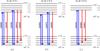 |
Fig. 1 Energy level diagrams for the Fe ii multiplets, UV1 (a), UV2 (b), and UV3 (c), where the ground and the excited states have multiple levels due to fine-structure splitting. Resonant transitions are shown in blue, and non-resonant transitions are shown in red. Whether non-resonant emission is likely to occur depends on the de-excitation rates and on the number (0, 1, or 2) of potential re-emission channels (Tang et al. 2014; Zhu et al. 2015). For example, the Fe ii λ2382 transition from the UV2 multiplet has no associated Fe ii* emission lines and thus behaves like a purely resonant transition (e.g., Lyα or Mg ii). |
A relatively new technique for studying galactic winds in emission relies on studying the signatures of photon scattering in low-ionization transitions since the pioneering work of Rubin et al. (2011). Photons absorbed in low-ionization metal lines (e.g., Si ii, C ii, Fe ii, Mg ii) can then lead to resonant or non-resonant re-emission. For resonant transitions, re-emitting absorbed photons through the same transition can give rise to P Cygni profiles with blue-shifted absorption and redshifted emission depending on the line optical depth, geometric factors, and the amount of emission infilling, as discussed in Prochaska et al. (2011). For non-resonant transitions, which are commonly indicated with an asterisk (e.g., Si ii*, C ii*, and Fe ii*), resonantly absorbed photons are re-emitted to one of the split levels of the ground state (e.g., Fig. 1). The resulting non-resonant emission lines, produced through continuum fluorescence, are typically a few Angstroms redward of their originating absorption lines. Resonant Mg ii (λλ2796,2803) emission and non-resonant Fe ii* (λ2365, λ2396, λ2612, λ2626) emission were first recognized as potential signatures of galactic winds in emission when seen together in the spectrum of a z = 0.694 star-forming galaxy (Rubin et al. 2011).
Characterizing the properties of galaxies that exhibit Fe ii* and Mg ii emission, typically with corresponding Fe ii and Mg ii absorption, is important for understanding the physical conditions that lead to outflows. Since Fe ii and Mg ii have similar ionization potentials, 7.90 eV and 7.65 eV respectively (NIST-ASD database; see also Table 2 from Zhu et al. 2015), they trace the same gas phase in the outflows. Galaxy properties, such as dust content, gas density, and inclination (for non-isotropic outflows), modulate the amount of resonant and non-resonant emission predicted in radiative transfer models of galactic outflows (Prochaska et al. 2011; Scarlata & Panagia 2015). In the local Universe, studies focused on resonant Na i D absorption and emission, which behave like Mg ii, have been able to investigate the connection between galaxy properties and outflows by leveraging a large statistical sample to trace, for example, how the emission and absorption varies with galaxy inclination (Chen et al. 2010) and by spatially resolving the emitting region for an individual galaxy (Rupke & Veilleux 2015).
Similar analyses for galaxies that exhibit Fe ii* and Mg ii emission are limited, because individual detections of non-resonant Fe ii* emission exist for only a handful of z ≲ 1 galaxies (e.g. Rubin et al. 2011; Coil et al. 2011; Martin et al. 2012; Finley et al. 2017). For instance, Finley et al. (2017) found that the Fe ii* spatial extent is 70% larger than that of the stellar continuum emission for an individual z = 1.29 galaxy observed with the Multi-Unit Spectroscopic Explorer (MUSE; Bacon et al. 2015) instrument. Such individual detections of non-resonant Fe ii* emission are rare, because slit losses may preclude detecting Fe ii* emission with traditional spectroscopy (Erb et al. 2012; Kornei et al. 2013; Scarlata & Panagia 2015). The MUSE integral field unit instrument eliminates the problem of slit losses and also offers a substantial gain in sensitivity, with a throughput of 35% end-to-end, including the atmosphere and telescope, at 7000 Å.
Since direct detections of individual galaxies with signatures of outflows in emission are difficult, several studies have instead focused on characterizing Fe ii* and Mg ii emission by creating composite spectra from ~ 100 or more z ~ 1 star-forming galaxies (Erb et al. 2012; Kornei et al. 2013; Tang et al. 2014; Zhu et al. 2015). These studies then look for trends between the emission strength and galaxy properties, such as stellar mass or dust extinction, by making composite spectra from sub-samples of galaxies. Erb et al. (2012) find that the most striking difference is between low and high-mass galaxies (median stellar masses of 1.8 × 10⁹ M⊙ and 1.5 × 10¹⁰ M⊙, respectively) with both stronger Mg ii emission and stronger Fe ii* emission in the low-mass composite spectrum. Interestingly, Erb et al. (2012) find more Fe ii* emission for galaxies with strong Mg ii emission.
After testing the emission strengths in 18 sets of composite spectra, Kornei et al. (2013) argue that dust extinction is the most important property influencing Fe ii* emission and is also a key property promoting Mg ii emission (more emission for lower dust extinction in both cases). Kornei et al. (2013) also find that galaxies with higher specific star-formation rates (sSFR) and lower stellar masses have stronger Mg ii emission, whereas galaxies with lower star formation rates (SFR) and larger [O ii] equivalent width measurements (W[ O ii ]) have stronger Fe ii* emission.
Unlike the two previous studies, Tang et al. (2014) do not find any strong trends with stellar mass, SFR, sSFR, or E(B−V). Tang et al. (2014) focus only on the Fe ii* emission and associated Fe ii absorption properties. Nonetheless, in an analysis of 8620 emission-line galaxies, Zhu et al. (2015) find that Fe ii* emission strength increases almost linearly with W[ O ii ].
A major caveat is that stacking offers little insight into how the emission might depend on wind orientation or geometry, given that composite spectra average out all galaxy inclinations. These geometrical effects can potentially be important, as radiative transfer models of outflows demonstrate (i.e., Prochaska et al. 2011; Scarlata & Panagia 2015). Characterizing how geometrical effects impact the emission signatures of outflows can only be performed with a sample of individual galaxies.
Thanks to the recent deep observations of the Hubble Ultra Deep Field South (UDF) with MUSE (Bacon et al. 2017, hereafter Paper I), we can now study and characterize a statistical sample of individual (unlensed) galaxies with Fe ii* in emission in order to understand whether geometrical effects play a role in Fe ii* emission (and/or Mg ii emission). We can also investigate how the prevalence of Fe ii* non-resonant emission varies with galaxy properties such as stellar mass, (specific) SFR, etc., thanks to deep multi-band photometry in the 3.15′ × 3.15′ mosaic of the UDF. This paper focuses on the emission line properties, and we will present the absorption line analysis and kinematics in a forthcoming paper.
The paper is organized as follows. In Sect. 2, we present the data and our selection criteria for Fe ii* emitters (and Mg ii emitters). In Sect. 3, we present our main results regarding the statistical properties of Fe ii* emitters. In Sect. 4, we show five representative cases. We review our findings in Sect. 5 and discuss possible physical processes producing the emission. Finally, we present our conclusions in Sect. 6. Throughout the paper, we assume a ΛCDM cosmology with Ωm = 0.3, ΩΛ = 0.7, and H0 = 70 km s-1 Mpc-1.
2. Data
2.1. MUSE observations
We used the 3.15′ × 3.15′ mosaic observations from nine MUSE pointings of the Hubble Ultra Deep Field South presented in Paper I. In summary, the MUSE UDF was observed during eight GTO runs over two years, from September 2014 to December 2015, for a total of 227 25-min exposures, leading to a depth of ~10 h per pointing. The central pointing (referred to as UDF-10) was observed for an additional 20 h, leading to a total depth of ~30 h in this region. The median PSF is 0.6′′, and the final 10-h data cube reaches a depth of ~2 × 10-18 (3σ) ergs s-1 cm-2 for line emitters (point sources). Further details about the observations and data reduction are presented in Paper I.
We used the MUSE UDF redshift catalog presented in Inami et al. (2017, hereafter Paper II). Paper II authors first identified sources in the MUSE data cube from objects with F775W ≤ 27 mag in the UVUDF photometric catalog (Rafelski et al. 2015) and from a blind search for emission lines objects using the ORIGIN software (Mary et al., in prep.). Paper II authors then combined a modified version of the AUTOZ (Baldry et al. 2014) cross-correlation algorithm with the MARZ software (Hinton et al. 2016) to determine the redshifts. While verifying the algorithm results, Paper II authors assigned a confidence level (CONFID) from 1 to 3 to each redshift measurement, where CONFID = 1 corresponds to the lowest confidence measurements and CONFID = 3 indicates the highest confidence measurements based on the presence of multiple absorption or emission features. They measured redshifts for 1439 objects in the 3.15′ × 3.15′ MUSE UDF mosaic, of which 192, 685 and 562 objects have redshift confidence 1, 2 and 3, respectively. Secure redshift measurements have CONFID > 1.
2.2. Sample selection
Since Finley et al. (2017) demonstrated the advantages of detecting Fe ii* from an individual galaxy, we took the MUSE UDF mosaic catalog (Paper II) as a basis to build a statistically significant sample of galaxies with Fe ii* emission/outflow signatures. Using this catalog, we first imposed a redshift range 0.85−1.50 designed such that we cover at least the [O ii] λλ3727,3729 line and the UV1 Fe ii multiplet, including the Fe ii* emission lines at λ2612 and λ2626. Although the MUSE spectral coverage for Fe ii* extends beyond z = 1.50, this upper limit ensures covering the [O ii] nebular line, which provides reliable systemic redshifts and a standardized approach to determining star-formation rates.
From the UDF mosaic catalog of 1439 objects with measured redshifts, 315 galaxies are in the redshift range 0.85−1.50. From these 315 galaxies, we kept 274 galaxies with redshift confidence CONFID > 1, of which 234 (40) have redshift confidence 3 (2), respectively. All but three of these galaxies are [O ii] emitters.
Within this sample, we visually inspected the spectra and searched for signatures of Fe ii*. We flagged a galaxy as an Fe ii* emitter if the spectrum shows any Fe ii* emission at λ2612 and λ2626 from the UV1 multiplet, at λ2396 from the UV2 multiplet, or at λ2365 from the UV3 multiplet, if covered1. Similar to the CONFID flag in the UDF mosaic catalog, we applied a quality control (qc) flag during the visual inspection. The qc > 1 flag indicates spectra with at least two Fe ii* emission lines (secure detections), whereas qc = 1 designates more marginal cases. As summarized in Table 1, we found 40 Fe ii* emitters in the UDF mosaic, 25 of which have qc > 1. All of the galaxies with Fe ii* emission also have Fe ii absorption.
In order to investigate the Mg ii emission properties of galaxies from the same parent sample and compare them with the Fe ii* emission properties, we simultaneously flagged the Mg ii profiles of the 274 galaxies in our redshift range as pure emission, P Cygni or pure absorption. The Mg ii λλ2796,2803 doublet is always covered within the 0.85−1.50 redshift range. In the UDF mosaic, we found 33 galaxies with pure Mg ii emission and 17 galaxies with P Cygni profiles.
UDF mosaic outflow signature galaxy sample.
3. Results for Fe ii* and Mg ii emitters
3.1. Redshift dependence of Fe II⋆ and Mg II emitter fractions
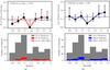 |
Fig. 2 Column a: bottom: redshift distribution for the Fe ii* emitters. The grey histogram shows the distribution for the full sample of 271 [O ii] emitters in the redshift range 0.85 < z < 1.50 (271 galaxies), and the red histogram shows the subpopulation of Fe ii* emitters with confidence flag qc > 1 (25 galaxies). White hatching indicates Fe ii* emitters that also have Mg ii emission or P Cygni profiles (9 galaxies). Top: the fraction of Fe ii* emitters for the eight redshift bins. Error bars on these fractions represent 68% confidence levels using Beta distributions as in Cameron (2011). The Fe ii*-emitter fraction is about 10% globally and is also consistent with a uniform distribution. Column b: bottom: redshift distribution for the Mg ii emitters. The grey histogram again shows the distribution for the full sample of [O ii] emitter galaxies, and the blue histogram shows the subpopulation of Mg ii emitters with confidence flag qc > 1 (33 galaxies). White hatching indicates Mg ii emitters that also have Fe ii* emission (9 galaxies). Top: the fraction of Mg ii emitters for each redshift bin with 68% confidence intervals. The Mg ii-emitter fraction is about 12% globally and is also consistent with a uniform distribution. |
We first look at the redshift distribution of our Fe ii* emitters to check whether they occur at a preferred redshift compared to the parent population of emission-line selected [O ii] emitters. The [O ii] emitters have a flux distribution that is approximately constant with redshift2.
We can expect that the redshift distribution will show a uniform relative fraction of Fe ii* emitters, if galactic outflows are ubiquitous in star-forming galaxies. However, Kornei et al. (2013) found that higher redshift galaxies have stronger Fe ii* emission in composite spectra from a sample of 212 star-forming galaxies with 0.2 < z < 1.3 (⟨ z ⟩ = 0.99), which the authors suggest could be due to galaxy properties evolving with redshift. If higher redshift galaxies produce stronger Fe ii* emission, then potentially we would detect more Fe ii* emitters at higher redshift.
Figure 2a traces the redshift distribution of galaxies across the range 0.85 < z < 1.50. In the bottom panel, the grey histogram shows the parent sample of 271 [O ii] emitter galaxies, and the red histogram shows the Fe ii* emitters. The top panel plots the fraction of Fe ii* emitters in each redshift bin with error bars representing the 68% confidence interval calculated from the Beta distribution following Cameron (2011). On average across the redshift range, the fraction of Fe ii* emitters is ~ 10%.
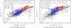 |
Fig. 3 Panel a: SFR–M⋆sequence for the 271 galaxies in our redshift range, (0.85 <z< 1.50), using SFR values from SED fitting. Panel b: SFR–M⋆sequence for the same galaxy sample using SFR values from L[O ii] fluxes with a dust correction following Kewley et al. (2004). In both panels, galaxies with only Fe ii* emission (only Mg ii emission or P Cygni profiles) are shown in red (blue). Galaxies with both Fe ii* emission and Mg ii emission or P Cygni profiles are shown in purple. Filled colored points indicate secure detections with qc> 1, and points with colored outlines indicate qc = 1 detections. The green filled region represents the main sequence in our redshift range determined by Schreiber et al. (2015) using a mass complete sample of 60 000 galaxies from the GOODS-Herschel and CANDELS-Herschel programs. The grey filled region represents the main sequence from Schreiber et al. (2015) extrapolated below their mass completeness. The green (grey) solid line with circular points represents the main sequence from Whitaker et al. (2014) over the redshift range z = [ 1.0−1.5 ] to M⋆= 109 M⊙ (extrapolated below their completeness), respectively. |
We test the observed fraction of Fe ii* emitters against the null hypothesis of a constant fraction over the redshift range using the proportions χ2 test from the Python statmodels module3. Based on the p-value of 0.76, the fraction of Fe ii* emitters does not show evidence of evolving across the redshift range 0.85 <z< 1.50. Since our redshift range does not extend to as low redshifts as the Kornei et al. (2013) sample, we may not be as sensitive to the effects of galaxy evolution that could produce less Fe ii* emission at lower redshift.
Similarly, Fig. 2b compares the redshift distribution of galaxies with Mg ii emission to the parent sample of [O ii] emitters. Based on the χ2 test, the relative fraction of Mg ii emitters also does not evolve with redshift across the redshift range 0.85 <z< 1.50. The average fraction is ~ 12%, comparable to the average fraction of Fe ii* emitters.
The redshift distributions for the Fe ii* and the Mg ii emitters are similar. We applied a Kolmogorov-Smirnov (KS) test to compare the redshift distributions for the galaxies with only Fe ii* emission and only Mg ii emission (excluding galaxies with both Fe ii* and Mg ii emission). The KS test results in a p-value of 0.79, suggesting that these two independent populations could be drawn from the same distribution. The phenomena producing Fe ii* and/or Mg ii emission occur in 18% of star-forming galaxies (49 / 271) observed in the MUSE UDF with a uniform distribution across the redshift range 0.85 <z< 1.50.
3.2. Fe II⋆ and Mg II emitters on the main sequence
We now turn towards the galaxy star-formation main sequence. This scaling relation between star-formation rate (SFR) and M⋆ is particularly important (Bouché et al. 2010; Mitra et al. 2017), since it applies for star-forming galaxies from the local Universe to z ≳ 4. Based on the work of numerous authors (e.g., Karim et al. 2011; Whitaker et al. 2014; Schreiber et al. 2015, among the more recent surveys), the galaxy main sequence is almost linear, except perhaps for M⋆> 1010 M⊙. Depending on where the Fe ii* and Mg ii emitters fall on this relation, the galaxy main sequence allows us to identify whether they are typical star-forming galaxies or if they instead belong to a subpopulation, such as starburst galaxies.
In order to estimate the stellar masses of the galaxies in the MUSE mosaic catalog, we performed standard spectral energy distribution (SED) fitting to the HST ACS and WFC3 photometry. We followed the same procedure as in Boogaard et al. (in prep.) and Paalvast et al. (in prep.). Briefly, this procedure applies the Fitting and Assessment of Synthetic Templates (FAST) algorithm (Kriek et al. 2009) using the 10 HST filters from Rafelski et al. (2015) and the Bruzual & Charlot (2003) library. We assumed exponential declining star formation histories with a Calzetti et al. (2000) attenuation law and a Chabrier (2003) initial mass function (IMF).
As described in Sect. 2.2, we selected galaxies with a maximum redshift 1.50, thereby ensuring that we cover [O ii]. We estimated the [O ii]-based SFRs from the luminosity L[ O ii ] ,obs using the method described in Kewley et al. (2004), which includes an empirical dust correction (their Eqs. (17) and (18)) and a metallicity correction (their Eq. (10) or (15)). The metallicity Z is estimated from the M⋆–Z relation of Zahid et al. (2014) and their formalism. To make the underlying Salpeter (1955) IMF for the [O ii]-based SFRs consistent with the Chabrier (2003) IMF used for the SED-based SFRs, we divided the [O ii]-based SFRs by a factor of 1.7.
The left (right) panel in Fig. 3 shows the SFR main sequence for our sample using SFR values from SED modeling (L[ O ii ] nebular models), which produce overall consistent main sequences. Figure 3 also indicates the main sequence that Schreiber et al. (2015) determined from a sample of 60 000 galaxies (mass complete down to ~ 109.8 M⊙) from the GOODS-Herschel and CANDELS-Herschel key-programs (green filled region) and that Whitaker et al. (2014) found for the redshift range z = [ 1.0−1.5 ] to M⋆= 109 M⊙ (green solid line with filled points). We extrapolated the results from Schreiber et al. (2015) and Whitaker et al. (2014) below their mass completeness to better compare with our sample (gray filled region and dark gray solid line with filled points, respectively). The UDF mosaic galaxies follow the expected trends down to ~ 108 M⊙. (See also Boogaard et al., in prep., for a discussion of the main sequence properties at the low-mass end.)
In Fig. 3, grey points indicate galaxies from our sample that have [O ii] emission, but no Fe ii* or Mg ii emission. Red (blue) points represent galaxies with only Fe ii* emission (only Mg ii emission), whereas purple points indicate galaxies that have both Fe ii* emission and Mg ii emission. Here we include galaxies with P Cygni profiles in the Mg ii emitter sample. This figure reveals that there is a strong apparent dichotomy between the populations of Fe ii* and Mg ii emitters. Indeed, below 109 M⊙ (and SFRs of ≲ 1 M⊙ yr-1), we observe Mg ii emission without accompanying Fe ii* emission, whereas, above 1010 M⊙ (and SFRs ≳ 10 M⊙ yr-1), we observe Fe ii* emission without accompanying Mg ii emission. Between these two regimes, we observe both Mg ii and Fe ii* emission, typically with Mg ii P Cygni profiles.
The dichotomy between Mg ii and Fe ii* emitters shown in Fig. 3 could be the result of a selection effect due to different sensitivities for Mg ii and Fe ii* in the spectra. Two potential selection effects could affect our sample, one that would prevent us from observing Mg ii emission in high-mass galaxies and another that would prevent us from detecting Fe ii* emission in low-mass galaxies. The first selection effect can be ruled out, because the spectra with the largest signal-to-noise are for galaxies with strong continua, typically at high-masses. Moreover, the ability to detect a constant flux/equivalent width does not depend on the continuum strength.
The second selection effect could explain the lack of Fe ii* emission at low mass and low SFR, because we need greater sensitivity in order to detect the Fe ii* emission, which is inherently weaker. Indeed, the strongest Fe ii* emission lines typically have rest-frame equivalent widths W0 between −0.5 and −1 Å, whereas the Mg ii emission lines have rest-frame equivalent widths −1 and −5 Å (see Feltre et al., in prep., for Mg ii emission properties). Examining the 30-h spectra from Mg ii emitters in the UDF-10, only one reveals Fe ii* emission and Fe ii absorption that were not flagged in the 10-h spectra (Sect. 4). However, even if we miss accompanying Fe ii* emission for the low-mass Mg ii emitters, we still observe a progression in Mg ii spectral signatures along the main sequence. We discuss physically motivated reasons for the Mg ii and Fe ii* spectral signatures in Sect. 5.
An important caveat to comparing the Mg ii/Fe ii* dichotomy in Fig. 3 with trends from composite spectra is that the samples used to create the composite spectra have almost no galaxies with M⋆= 108−9 M⊙ and SFR< 1 M⊙ yr-1, the regime where we observe Mg ii emission without accompanying Fe ii* emission. The composite spectra are only sensitive to the M⋆–SFR regime where we observe Fe ii* emission from the individual MUSE galaxies. Indeed, the regime that their sample covers may explain why Tang et al. (2014) do not see strong differences in the Fe ii* emission from their composite spectra split by stellar mass or SFR. Both Erb et al. (2012) and Kornei et al. (2013) find that composite spectra with strong Mg ii emission also have strong Fe ii* emission. Similar to many of the individual MUSE UDF galaxies with M⋆~ 109.5 M⊙, such as Fig. 8, these composite spectra show Fe ii* emission and Mg ii P Cygni profiles. Again, the M⋆–SFR regimes that the composite spectra studies probe implies that they are comparing samples of galaxies where we observe both Mg ii and Fe ii* emission from the MUSE galaxies.
3.3. Fe II⋆ and Mg II emission as a function of galaxy inclination and size
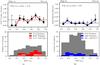 |
Fig. 4 Column a: bottom: axis ratio (b/a) distribution for the Fe ii* emitters from the HST Y-band. The grey histogram shows the distribution for 69 [O ii] emitters with SFR ≥ + 0.5 M⊙ yr-1, and the red histogram shows the subpopulation of Fe ii* emitters with confidence flag qc> 1 (23 galaxies). White hatching indicates Fe ii* emitters within this SFR range that also have Mg ii emission or P Cygni profiles (8 galaxies). Top: the fraction of Fe ii* emitters for the nine axis ratio bins. Error bars represent the 68% confidence interval as in Fig 1. Column b: bottom: axis ratio (b/a) distribution for the Mg ii emitters from the HST Y-band. The grey histogram shows the distribution for 133 [O ii] emitters with −0.5 M⊙ yr-1≤ SFR ≤ + 0.5 M⊙ yr-1, and the blue histogram shows the subpopulation of Mg ii emitters with confidence flag qc> 1 (17 galaxies). White hatching indicates Mg ii emitters within this SFR range that also have Fe ii* emission (1 galaxy). Top: the fraction of Mg ii emitters for the nine axis ratio bins. |
We took further advantage of the ancillary data available in the UDF area, and in particular of the size and morphological analysis by van der Wel et al. (2012). Briefly, van der Wel et al. (2012) performed single Sersic profile fits with the GALFIT Peng et al. (2010) algorithm on each of the available near-infrared bands (HF160W, JF125W and, for a subset, YF105W). The catalog includes the half-light radius (Reff), Sersic index n, axis ratio b/a, and position angle (PA) for each band. We used the Y-band for the analysis of axis ratios and sizes, since it typically has a higher signal-to-noise ratio (S/N), but found similar results with the other bands.
We explored whether the Fe ii* and Mg ii emitter galaxies have different inclinations or sizes than the [O ii] emitter galaxies for which these signatures are not detected. To focus on Fe ii* emitters, we took only galaxies from the parent sample with log SFR> + 0.5 M⊙ yr-1, using the SFR values from SED fitting. This SFR cut includes 69 [O ii] emitters, 23 of which have Fe ii* emission with qc> 1. Similarly, to focus on Mg ii emitters, we took only galaxies from the parent sample with −0.5 ≤ log SFR ≤ + 0.5 M⊙ yr-1. This SFR cut includes 133 [O ii] emitters, 17 of which have Mg ii emission with qc> 1. We compare the galaxy properties between Fe ii* or Mg ii emitters and [O ii] emitters within the same SFR range.
Figure 4 shows the axis ratio (b/a) distributions for the Fe ii* emitters and Mg ii emitters (bottom panels), as well as the emitter fractions (top panels). In both cases, χ2 statistical tests, as in Sect. 3.1, do not exclude uniform inclination distributions. Neither Fe ii* emission nor Mg ii emission appears to depend on the galaxy inclination.
Similarly, Fig. 5 shows the proper size (Reff) distributions for the Fe ii* emitters and Mg ii emitters (bottom panels) and their respective emitter fractions (top panels). Applying the χ2 statistical test to the emitter fractions does not exclude uniform size distributions for the Fe ii* and Mg ii emitters. Neither Fe ii* emission nor Mg ii emission appears to depend on the galaxy size.
Having established that Fe ii* emitters and Mg ii emitters do not have inclination or size distributions that are different from their parent populations, we also check whether the Fe ii* and Mg ii distributions are different from each other. We apply a Kolmogorov-Smirnov (K-S) test to compare the distributions from galaxies with only Fe ii* emission and only Mg ii emission, excluding galaxies that have both emission signatures, which are indicated with white cross hatching in the figures. The K-S test for the axis ratio distribution does not reject the possibility that the two samples are the same (p-value = 0.052), whereas the K-S test for the size distribution (p-value = 0.033) does imply that the samples are different. The distribution of Fe ii* emitters that do not have accompanying Mg ii emission peaks at larger sizes than the Mg ii emitter distribution, which is consistent with their higher stellar masses and SFRs.
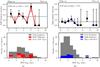 |
Fig. 5 Column a: bottom: proper size distribution (Reff) for Fe ii* emitters based on the HST Y-band semi-major axis measurements. The grey histogram shows the proper size distribution for 69 [O ii] emitters with SFR ≥ + 0.5 M⊙ yr-1. The red histogram shows the subpopulation of Fe ii* emitters with confidence flag qc> 1 (23 galaxies). White hatching indicates Fe ii* emitters within this SFR range that also have Mg ii emission or P Cygni profiles (8 galaxies). Top: the fraction of Fe ii* emitters. Error bars represent the 68% confidence interval as in Fig. 1. Column b: bottom: proper size distribution (Reff) for Mg ii emitters based on the HST Y-band semi-major axis measurements. The grey histogram shows the proper size distribution for 133 [O ii] emitters with −0.5 M⊙ yr-1≤ SFR ≤ + 0.5 M⊙ yr-1. The blue histogram shows the subpopulation of Mg ii emitters with confidence flag qc> 1 (17 galaxies). White hatching indicates Mg ii emitters within this SFR range that also have Fe ii* emission (1 galaxy). Top: the fraction of MgII emitters. |
3.4. Fe II⋆ and Mg II emission as a function of SFR surface density
The SFR surface density, ΣSFR, can be used as a criterion to determine whether a particular galaxy will drive an outflow, since higher SFRs per unit area will produce more pressure to potentially break through the galactic disk. The canonical threshold surface density for driving galactic outflows, ΣSFR> 0.1 M⊙ yr-1 kpc-2, is based on local starburst galaxies (Heckman 2002). However, both recent integral field spectroscopy results from local main sequence galaxies (Ho et al. 2016) and evidence of galactic outflows within the Milky Way Fermi Bubbles (Fox et al. 2015; Bordoloi et al. 2017) suggest that galaxies with lower ΣSFR values (ΣSFR ≈ 10-3−10-1.5 M⊙ yr-1kpc-2) can drive outflows. The threshold surface density may evolve with redshift (Sharma et al. 2016) and may also depend on the galaxy properties, especially the gas fraction (Newman et al. 2012). The threshold from the z ~ 2Newman et al. (2012) galaxy sample is ΣSFR = 1 M⊙ yr-1 kpc-2, an order of magnitude above the Heckman (2002) value. Constraints on the threshold surface density will improve as more studies are able to characterize both the outflow and the host galaxy properties.
We investigate whether there might be differences in the ΣSFR properties for the different populations of emitters. While we previously included P Cygni profiles in our Mg ii emitter sample, here we consider galaxies with P Cygni profiles and pure emission profiles separately. The pure Mg ii emitters have a range −2.6 < log ΣSFR< + 0.6 M⊙ yr-1 kpc-2 with mean value −1.1 ± 0.7 M⊙ yr-1 kpc-2. The Fe ii* emitters span a similar range, −2.7 < log ΣSFR< + 1.1 M⊙ yr-1 kpc-2, but with a higher mean value of −0.6 ± 0.7 M⊙ yr-1 kpc-2. Nearly all of the P Cygni profile Mg ii emitters also have Fe ii* emission, and they cover the most limited range, −1.3 < log ΣSFR< + 0.6 M⊙ yr-1 kpc-2, with mean value −0.3 ± 0.7 M⊙ yr-1 kpc-2. The pure Mg ii emitters have a lower mean ΣSFR value than the Fe ii* emitters or the Mg ii emitters with P Cygni profiles.
We evaluate whether the pure Mg ii emitters come from the same distribution as either the Fe ii* emitters or the Mg ii emitters with P Cygni profiles. In both cases, a K-S test rejects this hypothesis with p-values of 0.02 and 0.01, respectively. Pure Mg ii emitters have a different, lower ΣSFR distribution than galaxies with Fe ii* emission or Mg ii P Cygni profiles, and may be less likely to drive outflows.
4. Representative cases
In Sect. 3.2, we observed a dichotomy along the main sequence between galaxies with only Mg ii emission and galaxies with only Fe ii* emission. Furthermore, these emitters appear to show a progression where galaxies with M⋆≲ 109 M⊙ tend to have only Mg ii emission with no accompanying Mg ii or Fe ii absorption features, galaxies at the transition around M⋆~ 109.5 M⊙ have Mg ii P Cygni profiles with moderate Fe ii absorption with Fe ii* emission, and galaxies with M⋆≳ 1010 M⊙ have strong Mg ii and Fe ii absorption profiles with Fe ii* emission.
In order to investigate the 1D spectral properties of a representative sample, we selected galaxies that are detected in the deeper UDF-10 field in order to benefit from the higher signal-to-noise. Of the 25 Fe ii* emitters with qc> 1 in our UDF mosaic sample, seven are in the UDF-10 field, one of which is also detected with Mg ii emission. Of the 33 Mg ii emitters with qc> 1 in the mosaic, seven are in UDF-10 field. Two of these Mg ii emitters have P Cygni profiles. We summarize the characteristics of the 13 UDF-10 galaxies in Table 2.
Figures 6–10 transition from examples of galaxies with strong Mg ii absorption (ID08 and ID13) to a P Cygni profile (ID 32) to strong Mg ii emission (ID 33 and ID 56). All of these galaxies, except for ID 56, also have Fe ii* emission and Fe ii absorption. However, the weak Fe ii* emission and Fe ii absorption for ID33 are detected only in the UDF-10 spectrum, not flagged in the mosaic. The Fe ii* emitters flagged from the mosaic (Figs. 6–8) all have Fe ii and Mg ii in absorption, with possible emission infilling (see next section). Interestingly, the Mg ii emitters are often associated with a merging event, such as ID33, ID46 with ID92, and ID32 with ID121. Merging events may provoke outflows from these lower mass galaxies. The P Cygni profile from ID33 is further evidence of an outflow.
Galaxy properties for the Fe ii* and Mg ii emitters in the UDF-10 field, flagged with qc> 1 in the mosaic.
4.1. Emission signature properties from 1D spectra
For each of the seven Fe ii* emitters in the UDF-10 field, we measured the rest-frame equivalent widths for the Fe ii absorption and Fe ii* emission (Table 3) from the PSF-weighted sky-subtracted spectrum. For each spectrum, we fit the continuum with a cubic spline using a custom interactive python tool. From the normalized spectrum, we measured the rest-frame equivalent widths over velocity ranges that cover the full absorption/emission profiles. We calculated the equivalent widths by directly summing the flux and estimated uncertainties on these equivalent widths from the noise of the spectrum.
Before quantifying the equivalent widths, we note that Fe ii and Mg ii absorption lines may be affected by emission infilling (Prochaska et al. 2011; Scarlata & Panagia 2015; Zhu et al. 2015). Emission infilling occurs when an absorbed photon is re-emitted at the same wavelength, producing underlying emission that fills in the absorption profile and can shift the maximum absorption profile depth blueward. At its most extreme, emission infilling produces P Cygni profiles. Emission infilling affects some transitions more than others, depending on how likely it is for the absorbed photon to be re-emitted resonantly. From Zhu et al. (2015), the probability of emission infilling for each of the resonant Fe ii transitions is:  (1)where pres is the probability of emission infilling for purely resonant transitions that do not have associated non-resonant transitions, such as Fe ii λ2383 and Mg ii. For purely resonant transitions, the amount of emission infilling depends mainly on the degree of saturation, which in turn follows the absorption strength. Based on the elemental abundance and oscillator strength for each transition, the expected order for the absorption strength from Zhu et al. (2015) is:
 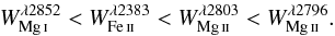 (2)The Mg ii doublet is therefore the most susceptible to emission infilling. Among the Fe ii transitions, Fe iiλ2383 is the most susceptible, while Fe ii λ2374 and λ2586 are the least susceptible to emission infilling. The radiative transfer models from Prochaska et al. (2011) and Scarlata & Panagia (2015) have shown that the amount of observed emission infilling also depends on several other factors, such as the outflow geometry and dust content.
We now quantify the amount of infilling for the Fe ii* emitters from the rest-frame equivalent width measurements using the Zhu et al. (2015) method. This method consists of comparing the observed rest-frame equivalent widths of the resonant lines detected in galaxy spectra to those seen as intervening absorption systems in quasar spectra (see their Fig. 12). The Fe ii λ2374 transition is the anchor point for this correction, since it is the least affected by emission infilling, as discussed in Tang et al. (2014) and Zhu et al. (2015). Here, we take the averaged rest-frame equivalent widths of resonant Fe ii and Mg ii absorption from a stacked spectrum of ~ 30 strong Mg ii absorber galaxies at 0.5 <z< 1.5 from Dutta et al. (2017, their Table 7) as a reference for intervening systems. The top panel of Fig. 11 shows the impact of the correction with diagonal black lines that trace the changes to the equivalent width values measured from each galaxy.
In Fig. 11, we follow Erb et al. (2012) and compare the amount of absorption on the x-axis with the total amount of emission (resonant and non-resonant) on the y-axis for the UV1 Fe ii λ2600 (top) and UV2 Fe ii λ2374 (bottom) transitions. Of the UV1, UV2, and UV3 Fe ii multiplets, these are the only transitions that have a single Fe ii* re-emission channel. For the UV2 Fe ii λ2374 transition (bottom), ~ 90% of the re-emission is through the non-resonant channel, Fe ii*λ2396, such that the resonant emission can be neglected. Resonant re-emission impacts the Fe ii λ2600 transitions more significantly, since only 13% of the re-emission is through the non-resonant Fe ii* λ2626 transition in a single-scattering approximation (Tang et al. 2014). The diagonal black line represents the case of photon-conservation, where all of the absorbed photons are re-observed as resonant and non-resonant emission.
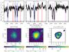 |
Fig. 6 UDF Galaxy ID 8 at z = 1.0948. Top row: sections of the MUSE spectrum with the UV2 and UV3 Fe ii multiplets (Fe ii λ2344, Fe ii*λ2365, Fe ii λλ2374,2382 and Fe ii*λ2396), the UV1 Fe ii multiplet (Fe ii λλ2586,2600 and Fe ii*λ2612,2626), and Mg ii λλ2796,2803 with Mg i λ2852. The blue (purple) dashed lines indicate the resonant Fe ii (Mg ii) transitions, and the red dashed lines show the non-resonant Fe ii* emission. Bottom row: HST F775W image and the MUSE [O ii] λ3729 flux map with an asinh scale, along with the corresponding MUSE S/N map with a threshold of S/N> 10. This galaxy is large and face-on. The spectrum shows Fe ii, Mg ii, and Mg i absorption features, with Fe ii* emission. |
 |
Fig. 7 UDF Galaxy ID 13 at z = 0.9973. Same panels as Fig. 6. For this redshift, the Fe ii UV2 and UV3 multiplets are not fully covered in the MUSE spectral range. Like the galaxy ID 8 (Fig. 6), this galaxy appears to be face on but disturbed, and the spectrum shows Fe ii, Mg ii, and Mg i absorption features, with Fe ii* emission. |
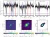 |
Fig. 8 UDF Galaxy ID 32 at z = 1.3071. Same panels as Fig. 6. This galaxy appears to be edge-on and is merging with UDF Galaxy ID 121. The spectrum shows Fe ii, Mg ii, and Mg i absorption features, with Fe ii* emission and a P Cygni profile for Mg ii. |
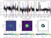 |
Fig. 9 UDF Galaxy ID 33 at z = 1.4156. Same panels as Fig. 6. Based on the HST image, this galaxy appears to be merging. The spectrum shows weak Fe ii absorption (most apparent for Fe ii λ2344 and Fe ii λ2374), weak Fe ii* emission, and strong Mg ii emission. |
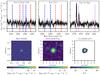 |
Fig. 10 UDF Galaxy ID 56 at z = 1.3061. Same panels as Fig. 6. This galaxy is compact, and the spectrum shows only Mg ii emission, without Fe ii absorption or Fe ii* emission. The Mg ii absorption creating a slight P Cygni profile for this Mg ii emitter is detectable only in the UDF-10 spectrum. |
Rest-Frame equivalent width measurements for the seven Fe ii* emitters in the UDF-10 field (not corrected for emission infilling).
The solid colored points in Fig. 11 indicate the Fe ii* emitter equivalent widths for the UDF-10 sub-sample, along with the HDFS-ID13 z = 1.29 galaxy from Finley et al. (2017). Here, the observed resonant Fe ii absorption and emission equivalent widths (Table 3) are corrected using the infilling emission correction for the UV1 Fe ii λ2600 transition as discussed earlier. The solid black lines trace the difference between the measured and the corrected values. This infilling correction moves points parallel to the photon-conservation line, since accounting for emission infilling increases both the amount of absorption and the total amount of emission. The galaxies that are furthest from the photon conservation line are all larger face-on galaxies, characteristics that facilitate detecting absorption.
The diamonds in Fig. 11 represent theoretical predictions for the UV1 Fe ii λ2600 and Fe ii λ2626 transitions from the Prochaska et al. (2011) radiative transfer models of galactic outflows. No models are available for the UV2 Fe ii λ2374 transition. The fiducial model (black outlined diamond) assumes a dust-free, isotropic radial outflow with the gas density decreasing as r-2 and the velocity decreasing as r. Variations on the fiducial model test additional gas density and velocity laws (gray diamonds), and these models, like the fiducial model, follow the photon-conservation line. Some of the isotropic, dust-free models predict Fe ii λ2600 absorption values of W0 ~ 3−4 Å, similar to what is observed for the Fe ii* emitter galaxies. However, they all over-predict the corresponding total amount of emission.
The diamonds with colored outlines in Fig. 11 show models that deviate from the photon-conservation line and predict more absorption than emission. These models test the effects of dust extinction or collimated outflow geometries. Increasing the dust extinction in an isotropic outflow model (red and orange outlined diamonds) decreases the total amount of re-emission and produces a nearly vertical offset from the photon-conservation line. The impact of dust extinction becomes more pronounced after introducing a component that represents the interstellar medium (ISM), i.e., gas that is centralized and lacks a significant radial velocity. Adding only the ISM component shifts the model predictions along the photon-conservation line (purple outlined diamond), whereas including an ISM component plus τdust = 1 dust extinction (magenta outlined diamond) significantly decreases the total amount of re-emission.
Finally, modifying the outflow geometry such that it becomes increasingly collimated (θb = 80°,45°, green outlined diamonds) also moves the model predictions away from the photon-conservation line. Interestingly, the highly collimated outflow model (light green outlined diamond) and the isotropic outflow with an ISM component and dust extinction (magenta outlined diamond) both occupy the same parameter space in this figure, despite having very different physical properties. Additional modeling is required to better understand the combined effects of dust extinction and geometry.
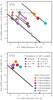 |
Fig. 11 Photon-conservation diagnostics for the two resonant Fe ii transitions, λ2374 UV2 (bottom) and λ2600 UV1 (top), with only one Fe ii* re-emission channel (Fe ii*λ2396 and Fe ii*λ2626 respectively). In both panels, the x-axis is the resonant absorption equivalent width, and the y-axis is the total re-emission equivalent width from the resonant and non-resonant transitions. However, resonant re-emission (emission infilling) is negligible for the Fe ii λ2374 transition (Tang et al. 2014; Zhu et al. 2015). The diagonal black line represents photon-conservation between emission and absorption processes. The solid colored points represent the Fe ii* emitters from this sample with the emission infilling correction (see text). The black lines associated with these points in the top panel trace the difference between the measured and corrected equivalent width values. The solid diamonds represent theoretical predictions from the radiative transfer models of Prochaska et al. (2011). Gray diamonds indicate isotropic outflow models, which all respect photon conservation, and the diamonds with colored outlines show variations to the geometry and dust content that decrease the total amount of re-emission. |
Comparing the top and bottom panels of Fig. 11 shows that, irrespective of the infilling correction, the observed data for the Fe ii λ2600 transition is more offset from the photon-conservation line than the Fe ii λ2374 transition from the same galaxy. Dust extinction can account for both the offset from the photon-conservation line as well as why this offset is more pronounced for the Fe ii λ2600 transition. The Fe ii λ2600 transition is more sensitive to dust extinction, since this transition is more likely to produce resonant re-emission than Fe ii* λ2626 non-resonant emission following a single scattering process (see Tang et al. 2014, their Fig. 5). The resonant re-emission undergoes multiple scatterings, and photons that repeatedly scatter also have multiple chances to be absorbed by dust, a process known as resonant trapping. Conversely, the Fe ii λ2374 transition is less sensitive to dust extinction and resonant trapping, since nearly all of the re-emission is through the non-resonant Fe ii*λ2396 channel. Thus, for a given galaxy, the Fe ii λ2600 transition has a larger offset from the photon-conservation line than the Fe ii λ2374 transition, due to its greater sensitivity to dust extinction.
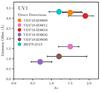 |
Fig. 12 Emission offset versus dust extinction from SED fitting. For each galaxy from Fig. 11, the emission offset measures the vertical distance between the total emission from Fe ii λ2600 and Fe ii*λ2626 in the UV1 multiplet and the photon-conservation line. |
Figure 12 quantifies the vertical offset between the total Fe ii λ2600 and Fe ii* λ2626 re-emission from each galaxy and the photon-conservation line and suggests that the emission offset might increase with increasing dust extinction. The emission offset and dust extinction in Fig. 12 have a Pearson correlation coefficient of 0.63, but more data points are necessary to solidify the trend. The dust extinction estimate, AV, is from SED modeling (Sect. 3.2), which is robust for the UDF-10 galaxies given the deep HST imaging across multiple bands. Dust extinction is potentially a significant factor contributing to the offset between the observed emission and the photon-conservation line, in agreement with the Prochaska et al. (2011) radiative transfer models. The other significant factor driving the offset may be geometric effects, as discussed above. However, more models are required to determine how to best characterize the impact of geometric effects and compare this impact with that of dust extinction.
5. Discussion
Along the SFR main sequence (Fig. 3), the emission signatures vary from only Mg ii emission, to both Mg ii and Fe ii* emission, to only Fe ii* emission. We propose that this progression is physically motivated, with distinct physical processes producing the emission signatures at the two extremes of the SFR main sequence.
The physical processes that produce Fe ii* emission at the high mass, high SFR end and Mg ii emission at the low mass, low SFR end may be distinct. For Fe ii*, the physical process driving non-resonant emission is continuum fluorescence (Prochaska et al. 2011)4. For Mg ii, two main physical processes can give rise to emission in low mass galaxies: resonant scattering following continuum absorption or nebular emission in H ii regions5. Whether Mg ii emission in a particular galaxy is predominantly due to continuum scattering or nebular emission may depend on the strength of the stellar continuum, which we quantify with the HST F606W magnitude.
The low mass, low SFR galaxies with only Mg ii emission detected have weak stellar continua (mF606W ≈ 26). When fewer continuum photons are available to undergo absorption, less continuum scattering and less Fe ii* emission occurs. Galaxies with weak stellar continua therefore do not have significant absorption or Fe ii* emission features; instead, they have Mg ii emission as the predominant feature. The Mg ii emission has median equivalent width values of W0,2796 = −4.1 Å and W0,2803 = −1.7 Å, with a typical error (median 1σ measurement error) of 1.3 Å. Mg ii emission alone, without accompanying Fe ii* emission, likely comes predominantly from H ii regions, rather than from continuum scattering. Based on photoionization modeling, most Mg ii emission in 1 <z< 2 star-forming galaxies with outflow signatures is from H ii regions, but these H ii regions would need higher ionization parameters to directly produce the Fe ii* emission (Erb et al. 2012).
As the strength of the stellar continuum increases (mF606W ≈ 24.6), the galaxy spectra show Fe ii absorption and Fe ii* emission, along with Mg ii P Cygni profiles. The Mg ii P Cygni profiles, which are overall dominated by absorption, have median equivalent width values of W0,2796 = + 0.7 Å and W0,2803 = + 1.1 Å, with a typical error of 0.5 Å. The appearance of Mg ii P Cygni profiles suggests that continuum scattering is the physical process driving Mg ii emission in these galaxies. Previously studied direct detections of Fe ii* emission and Mg ii P Cygni profiles in individual galaxies (Rubin et al. 2011; Martin et al. 2013) demonstrate that continuum scattering in galactic outflows produce these emission signatures.
Finally, the high mass, high SFR galaxies with Fe ii* emission but no accompanying Mg ii emission have the strongest stellar continua of the sample (mF606W ≈ 23.6) and strong Fe ii and Mg ii absorption features. The Mg ii absorptions have median equivalent width values of W0,2796 = + 2.7 Å and W0,2803 = + 2.2 Å, with a typical error of 0.3 Å. In the case of strong absorption, the absorbed continuum photons can become resonantly trapped, i.e., they undergo so many scattering events that few photons escape as resonant emission. Resonant trapping suppresses emission from the Mg ii λλ2796,2803 transitions, which are purely resonant with no non-resonant channels. However, resonant trapping promotes Fe ii* emission, since more scattering events provide more opportunities for photons to escape through a non-resonant channel. Due to resonant trapping, stronger absorption features imply weaker Mg ii emission.
Since dust extinction enhances resonant trapping, we can expect to see more Mg ii emission from galaxies with less dust. Dust extinction increases with the galaxy mass and SFR (e.g., Kewley et al. 2004; Brinchmann et al. 2004), so the low-mass, low-SFR Mg ii emitters likely have the least amount of dust. Indeed, Feltre et al. (in prep.) find lower extinction values for the MUSE UDF Mg ii emitters compared to Mg ii absorbers. Similarly, dust extinction is potentially the driving factor that determines the strength of Fe ii* emission (Kornei et al. 2013). While resonant trapping from strong absorption components enhances the Fe ii* emission, dust extinction from these same components mitigates this enhancement. We can expect a trend between the dust extinction and the amount of re-emission (explored in Fig. 12), which may become clearer if we considered only the ISM component.
The physical process driving the Mg ii and Fe ii* emission signatures helps determine whether these signatures trace galactic outflows. Attributing Mg ii emission without accompanying Fe ii* to nebular emission, rather than continuum scattering, means that Mg ii emission alone likely traces H ii regions within the galaxy and not outflows. Indeed, galaxies with pure Mg ii emission profiles have lower SFR surface densities than those with P Cygni profiles or Fe ii* emission. The P Cygni profiles and Fe ii* emission signatures likely arise from continuum scattering and fluorescence, since all of these galaxies also have absorption features. Continuum scattering and fluorescence can produce Fe ii* emission either with Mg ii P Cygni profiles or with no accompanying Mg ii emission, in the case of strong resonant trapping. Among the emission signatures, Fe ii* emission or Mg ii P Cygni profiles are therefore the best candidates for tracing outflows. To confirm that the Fe ii* and Mg ii P Cygni profile signatures are associated with galactic outflows, we will need to investigate the kinematics of the absorbing and emitting gas and map the spatial extent, as for the MUSE HDFS galaxy ID#13 (Finley et al. 2017).
6. Conclusions
Non-resonant Fe ii* emission and Mg ii P Cygni profiles can potentially trace galactic winds in emission and provide useful constraints on wind models. From the 3.15′ × 3.15′ mosaic of the Hubble Ultra Deep Field (UDF) obtained with the VLT/MUSE integral field spectrograph, we identify a statistical sample of 40 Fe ii* emitters from a sample of 271 [O ii] emitters with reliable redshifts in the range z = 0.85−1.50 down to 2 × 10-18 (3σ) ergs s-1 cm-2. From the same parent sample, we identify 50 Mg ii emitters, with both pure emission and P Cygni profiles. Applying a confidence quality flag (qc > 1), we have 25 Fe ii* emitters and 33 Mg ii emitters, with 9 galaxies that show both emission signatures.
With this sample, we explore the characteristics of galaxies with Fe ii* and/or Mg ii emission. Our main results are:
-
Approximately 10% of galaxies in the redshift range z = 0.85−1.50 have Fe ii* or Mg ii emission with no evidence of an evolution with redshift (Fig. 2).
-
The Fe ii* and Mg ii emitters follow the galaxy main sequence (Fig. 3), but show a strong dichotomy. Galaxies below 109M⊙ (and SFRs of ≲ 1M⊙ yr-1), have Mg ii emission without accompanying Fe ii* emission, whereas galaxies above 1010M⊙ (and SFRs ≳ 10M⊙ yr-1) have Fe ii* emission without accompanying Mg ii emission. Between these two regimes, galaxies have both Mg ii and Fe ii* emission, typically with Mg ii P Cygni profiles.
-
The inclination and size distributions of the Fe ii* and Mg ii emitters are not different from parent samples of [O ii] emitters with similar SFRs, but the size distribution for galaxies with only Mg ii emission is different from that of galaxies with only Fe ii* emission. Consistent with the dichotomy in the SFR-M⋆ sequence, the galaxies with only Fe ii* emission tend to be larger.
-
Splitting the Mg ii emitter sample by profile type reveals that the galaxies with pure Mg ii emission profiles have a SFR surface density distribution that is different from galaxies with Mg ii P Cygni profiles or Fe ii* emission. The pure Mg ii emitters have a lower mean value of −1.1M⊙ yr-1kpc-2, compared to −0.3 or −0.5M⊙ yr-1kpc-2 for Mg ii P Cygni profiles or Fe ii* emission, and therefore may be less likely to drive outflows.
-
Representative cases from the UDF-10 field (Figs. 6–10) highlight the progression of Mg ii spectral signatures from pure emission to P Cygni profiles to pure absorption, which is likely the result of resonant trapping as the amount of ISM gas and dust increases with stellar mass and SFR. The representative cases also demonstrate that Fe ii* emission consistently occurs with Fe ii and Mg ii absorptions, including P Cygni profiles, whereas pure Mg ii emission tends to occur without Fe ii absorption or Fe ii* emission.
-
The UV1 Fe ii λ2600 transition and its associated Fe ii*λ2626 transition are more strongly affected by resonant trapping than the UV2 Fe ii λ2374 transition with Fe ii*λ2396. Consequently, the former are more sensitive to dust extinction, which offsets the emission vertically from the photon-conservation line (Fig. 11) and potentially increases as the emission offset increases (Fig. 12).
Identifying a statistical sample of individual z ~ 1 galaxies with Fe ii* emission from MUSE observations creates new opportunities to characterize galactic outflows. We will build on the analysis presented in this paper by decomposing the absorption profiles into systemic and blueshifted components to obtain outflow velocities. We will also exploit the IFU observations to map the extent of the Fe ii* and Mg ii emission, as in Finley et al. (2017).
In the MUSE UDF spectra, we do not detect Fe ii*emission at λ2381 or λ2632. The Fe ii* λ2381 transition is blended with the Fe ii λ2382 absorption.
The parent population of [O ii] emitter galaxies appears non-uniform, since skyline emission at redder wavelengths interferes with our ability to detect [O ii] emitters towards higher redshifts. See Brinchmann et al. (2017) for a discussion of redshift completeness in the MUSE UDF catalog.
Through Monte Carlo testing, we verified that the proportions χ2 follows a χ2 distribution even in the low-count regime, unlike the Pearson χ2.
While it is also possible to produce Fe ii* emission through indirect UV pumping or collisional excitation, indirect UV pumping requires close proximity (< 100 pc) to strong UV sources, and collisional excitation requires high density environments with > 105 cm-2.
AGN or shocks from merger events can also produce Mg ii emission.
Acknowledgments
We thank for referee for feedback that helped to improve the paper. Based on observations collected at the European Organisation for Astronomical Research in the Southern Hemisphere under ESO programs 094.A-0289(B), 095.A-0010(A), 096.A-0045(A) and 096.A-0045(B). This work has been carried out thanks to the support of the ANR FOGHAR (ANR-13-BS05-0010-02), the OCEVU Labex (ANR-11-LABX-0060), and the A*MIDEX project (ANR-11-IDEX-0001-02) funded by the “Investissements d’avenir” French government program. RB and AF acknowledge support from the ERC advanced grant 339659-MUSICOS. JB is supported by FCT through Investigador FCT contract IF/01654/2014/CP1215/CT0003, by Fundação para a Ciência e a Tecnologia (FCT) through national funds (UID/FIS/04434/2013), and by FEDER through COMPETE2020 (POCI-01-0145-FEDER-007672). BE acknowledges support from the “Programme National de Cosmologie and Galaxies” (PNCG) of CNRS/INSU, France. JR acknowledges support from the ERC starting grant 336736-CALENDS.
References
- Aguirre, A., Hernquist, L., Schaye, J., et al. 2001, ApJ, 561, 521 [NASA ADS] [CrossRef] [Google Scholar]
- Arribas, S., Colina, L., Bellocchi, E., Maiolino, R., & Villar-Martín, M. 2014, A&A, 568, A14 [NASA ADS] [CrossRef] [EDP Sciences] [Google Scholar]
- Bacon, R., Brinchmann, J., Richard, J., et al. 2015, A&A, 575, A75 [NASA ADS] [CrossRef] [EDP Sciences] [Google Scholar]
- Bacon, R., Conseil, S., Mary, D., et al. 2017, A&A, 608, A1 (MUSE UDF, SI Paper I) [NASA ADS] [CrossRef] [EDP Sciences] [Google Scholar]
- Baldry, I. K., Alpaslan, M., & Bauer, A. 2014, MNRAS, 441, 2440 [NASA ADS] [CrossRef] [Google Scholar]
- Bordoloi, R., Lilly, S. J., Kacprzak, G. G., & Churchill, C. W. 2014, ApJ, 784, 108 [NASA ADS] [CrossRef] [Google Scholar]
- Bordoloi, R., Fox, A. J., Lockman, F. J., et al. 2017, ApJ, 834, 191 [NASA ADS] [CrossRef] [Google Scholar]
- Bouché, N., Dekel, A., Genzel, R., et al. 2010, ApJ, 718, 1001 [NASA ADS] [CrossRef] [Google Scholar]
- Brinchmann, J., Charlot, S., White, S. D. M., et al. 2004, MNRAS, 351, 1151 [NASA ADS] [CrossRef] [Google Scholar]
- Brinchmann, J., Inami, H., Bacon, R., et al. 2017, A&A, 608, A3 (MUSE UDF SI, Paper III) [NASA ADS] [CrossRef] [EDP Sciences] [Google Scholar]
- Bruzual, G., & Charlot, S. 2003, MNRAS, 344, 1000 [NASA ADS] [CrossRef] [Google Scholar]
- Calzetti, D., Armus, L., Bohlin, R. C., et al. 2000, ApJ, 533, 682 [NASA ADS] [CrossRef] [Google Scholar]
- Cameron, E. 2011, PASA, 28, 128 [NASA ADS] [CrossRef] [Google Scholar]
- Chabrier, G. 2003, ApJ, 586, L133 [NASA ADS] [CrossRef] [Google Scholar]
- Chen, Y.-M., Tremonti, C. A., Heckman, T. M., et al. 2010, AJ, 140, 445 [NASA ADS] [CrossRef] [Google Scholar]
- Chisholm, J., Tremonti, C. A., Leitherer, C., et al. 2015, ApJ, 811, 149 [NASA ADS] [CrossRef] [Google Scholar]
- Coil, A. L., Weiner, B. J., Holz, D. E., et al. 2011, ApJ, 743, 46 [NASA ADS] [CrossRef] [Google Scholar]
- Dutta, R., Srianand, R., Gupta, N., et al. 2017, MNRAS, 465, 4249 [NASA ADS] [CrossRef] [Google Scholar]
- Erb, D. K., Quider, A. M., Henry, A. L., & Martin, C. L. 2012, ApJ, 759, 26 [NASA ADS] [CrossRef] [Google Scholar]
- Finlator, K., & Davé, R. 2008, MNRAS, 385, 2181 [NASA ADS] [CrossRef] [Google Scholar]
- Finley, H., Bouché, N., Contini, T., et al. 2017, A&A, 605, A118 [NASA ADS] [CrossRef] [EDP Sciences] [Google Scholar]
- Ford, A. B., Werk, J. K., Davé, R., et al. 2016, MNRAS, 459, 1745 [NASA ADS] [CrossRef] [Google Scholar]
- Fox, A. J., Bordoloi, R., Savage, B. D., et al. 2015, ApJ, 799, L7 [NASA ADS] [CrossRef] [Google Scholar]
- Genzel, R., Newman, S., Jones, T., et al. 2011, ApJ, 733, 101 [Google Scholar]
- Grimes, J. P., Heckman, T., Strickland, D., & Ptak, A. 2005, ApJ, 628, 187 [NASA ADS] [CrossRef] [Google Scholar]
- Harikane, Y., Ouchi, M., Yuma, S., et al. 2014, ApJ, 794, 129 [NASA ADS] [CrossRef] [Google Scholar]
- Heckman, T. M. 2002, in Extragalactic Gas at Low Redshift, eds. J. S. Mulchaey, & J. T. Stocke, ASP Conf. Ser., 254, 292 [Google Scholar]
- Heckman, T. M., Alexandroff, R. M., Borthakur, S., Overzier, R., & Leitherer, C. 2015, ApJ, 809, 147 [NASA ADS] [CrossRef] [Google Scholar]
- Hinton, S. R., Davis, T. M., Lidman, C., Glazebrook, K., & Lewis, G. F. 2016, Astron. Comput., 15 [Google Scholar]
- Ho, I.-T., Medling, A. M., Bland-Hawthorn, J., et al. 2016, MNRAS, 457, 1257 [NASA ADS] [CrossRef] [Google Scholar]
- Inami, H., Bacon, R., Brinchmann, J., et al. 2017, A&A, 608, A2 (MUSE UDF SI, Paper II) [NASA ADS] [CrossRef] [EDP Sciences] [Google Scholar]
- Karim, A., Schinnerer, E., Martínez-Sansigre, A., et al. 2011, ApJ, 730, 61 [NASA ADS] [CrossRef] [Google Scholar]
- Kewley, L. J., Geller, M. J., & Jansen, R. A. 2004, AJ, 127, 2002 [NASA ADS] [CrossRef] [Google Scholar]
- Kornei, K. A., Shapley, A. E., Martin, C. L., et al. 2013, ApJ, 774, 50 [NASA ADS] [CrossRef] [Google Scholar]
- Kriek, M., van Dokkum, P. G., Labbé, I., et al. 2009, ApJ, 700, 221 [NASA ADS] [CrossRef] [Google Scholar]
- Lehnert, M. D., & Heckman, T. M. 1995, ApJS, 97, 89 [NASA ADS] [CrossRef] [Google Scholar]
- Lehnert, M. D., & Heckman, T. M. 1996, ApJ, 462, 651 [NASA ADS] [CrossRef] [Google Scholar]
- Lehnert, M. D., Heckman, T. M., & Weaver, K. A. 1999, ApJ, 523, 575 [NASA ADS] [CrossRef] [Google Scholar]
- Lilly, S. J., Carollo, C. M., Pipino, A., Renzini, A., & Peng, Y. 2013, ApJ, 772, 119 [NASA ADS] [CrossRef] [Google Scholar]
- Martin, C. L. 1999, ApJ, 513, 156 [NASA ADS] [CrossRef] [Google Scholar]
- Martin, C. L., Shapley, A. E., Coil, A. L., et al. 2013, ApJ, 770, 41 [NASA ADS] [CrossRef] [Google Scholar]
- Martin, C. L., Shapley, A. E., Coil, A. L., et al. 2012, ApJ, 760, 127 [NASA ADS] [CrossRef] [Google Scholar]
- Mitra, S., Davé, R., Simha, V., & Finlator, K. 2017, MNRAS, 464, 2766 [NASA ADS] [CrossRef] [Google Scholar]
- Newman, S. F., Genzel, R., Förster-Schreiber, N. M., et al. 2012, ApJ, 761, 43 [NASA ADS] [CrossRef] [Google Scholar]
- Oppenheimer, B. D., & Davé, R. 2008, MNRAS, 387, 577 [NASA ADS] [CrossRef] [Google Scholar]
- Peng, C. Y., Ho, L. C., Impey, C. D., & Rix, H.-W. 2010, AJ, 139, 2097 [NASA ADS] [CrossRef] [Google Scholar]
- Prochaska, J. X., Kasen, D., & Rubin, K. 2011, ApJ, 734, 24 [NASA ADS] [CrossRef] [Google Scholar]
- Rafelski, M., Teplitz, H. I., Gardner, J. P., et al. 2015, AJ, 150, 31 [NASA ADS] [CrossRef] [Google Scholar]
- Rubin, K. H. R., Weiner, B. J., Koo, D. C., et al. 2010, ApJ, 719, 1503 [NASA ADS] [CrossRef] [Google Scholar]
- Rubin, K. H. R., Prochaska, J. X., Ménard, B., et al. 2011, ApJ, 728, 55 [NASA ADS] [CrossRef] [Google Scholar]
- Rubin, K. H. R., Prochaska, J. X., Koo, D. C., et al. 2014, ApJ, 794, 156 [NASA ADS] [CrossRef] [Google Scholar]
- Rupke, D. S. N., & Veilleux, S. 2013, ApJ, 768, 75 [NASA ADS] [CrossRef] [Google Scholar]
- Rupke, D. S. N., & Veilleux, S. 2015, ApJ, 801, 126 [Google Scholar]
- Salpeter, E. E. 1955, ApJ, 121, 161 [Google Scholar]
- Scarlata, C., & Panagia, N. 2015, ApJ, 801, 43 [NASA ADS] [CrossRef] [Google Scholar]
- Schreiber, C., Pannella, M., Elbaz, D., et al. 2015, A&A, 575, A74 [NASA ADS] [CrossRef] [EDP Sciences] [Google Scholar]
- Sharma, M., Theuns, T., Frenk, C., et al. 2016, MNRAS, 458, L94 [NASA ADS] [CrossRef] [Google Scholar]
- Silk, J., & Mamon, G. A. 2012, Res. Astron. Astrophys., 12, 917 [NASA ADS] [CrossRef] [Google Scholar]
- Soto, K. T., & Martin, C. L. 2012, ApJS, 203, 3 [NASA ADS] [CrossRef] [EDP Sciences] [Google Scholar]
- Steidel, C. C., Erb, D. K., Shapley, A. E., et al. 2010, ApJ, 717, 289 [NASA ADS] [CrossRef] [Google Scholar]
- Strickland, D. K., & Heckman, T. M. 2009, , 29 [Google Scholar]
- Strickland, D. K., & Stevens, I. R. 1999, MNRAS, 306, 43 [NASA ADS] [CrossRef] [Google Scholar]
- Strickland, D. K., Heckman, T. M., Colbert, E. J. M., Hoopes, C. G., & Weaver, K. A. 2004, ApJS, 151, 193 [NASA ADS] [CrossRef] [Google Scholar]
- Tang, Y., Giavalisco, M., Guo, Y., & Kurk, J. 2014, ApJ, 793, 92 [NASA ADS] [CrossRef] [Google Scholar]
- Tremonti, C. A., Heckman, T. M., Kauffmann, G., et al. 2004, ApJ, 613, 898 [NASA ADS] [CrossRef] [Google Scholar]
- van der Wel, A., Bell, E. F., Häussler, B., et al. 2012, ApJS, 203, 24 [NASA ADS] [CrossRef] [Google Scholar]
- Veilleux, S., Shopbell, P. L., Rupke, D. S., Bland-Hawthorn, J., & Cecil, G. 2003, AJ, 126, 2185 [NASA ADS] [CrossRef] [Google Scholar]
- Veilleux, S., Cecil, G., & Bland-Hawthorn, J. 2005, ARA&A, 43, 769 [Google Scholar]
- Weiner, B. J., Coil, A. L., Prochaska, J. X., et al. 2009, ApJ, 692, 187 [NASA ADS] [CrossRef] [Google Scholar]
- Westmoquette, M. S., Clements, D. L., Bendo, G. J., & Khan, S. A. 2012, MNRAS, 424, 416 [NASA ADS] [CrossRef] [Google Scholar]
- Whitaker, K. E., Franx, M., Leja, J., et al. 2014, ApJ, 795, 104 [NASA ADS] [CrossRef] [MathSciNet] [Google Scholar]
- Zahid, H. J., Dima, G. I., Kudritzki, R.-P., et al. 2014, ApJ, 791, 130 [NASA ADS] [CrossRef] [Google Scholar]
- Zhu, G. B., Comparat, J., Kneib, J.-P., et al. 2015, ApJ, 815, 48 [NASA ADS] [CrossRef] [Google Scholar]
All Tables
Galaxy properties for the Fe ii* and Mg ii emitters in the UDF-10 field, flagged with qc> 1 in the mosaic.
Rest-Frame equivalent width measurements for the seven Fe ii* emitters in the UDF-10 field (not corrected for emission infilling).
All Figures
|
Fig. 1 Energy level diagrams for the Fe ii multiplets, UV1 (a), UV2 (b), and UV3 (c), where the ground and the excited states have multiple levels due to fine-structure splitting. Resonant transitions are shown in blue, and non-resonant transitions are shown in red. Whether non-resonant emission is likely to occur depends on the de-excitation rates and on the number (0, 1, or 2) of potential re-emission channels (Tang et al. 2014; Zhu et al. 2015). For example, the Fe ii λ2382 transition from the UV2 multiplet has no associated Fe ii* emission lines and thus behaves like a purely resonant transition (e.g., Lyα or Mg ii). |
| In the text | |
|
Fig. 2 Column a: bottom: redshift distribution for the Fe ii* emitters. The grey histogram shows the distribution for the full sample of 271 [O ii] emitters in the redshift range 0.85 < z < 1.50 (271 galaxies), and the red histogram shows the subpopulation of Fe ii* emitters with confidence flag qc > 1 (25 galaxies). White hatching indicates Fe ii* emitters that also have Mg ii emission or P Cygni profiles (9 galaxies). Top: the fraction of Fe ii* emitters for the eight redshift bins. Error bars on these fractions represent 68% confidence levels using Beta distributions as in Cameron (2011). The Fe ii*-emitter fraction is about 10% globally and is also consistent with a uniform distribution. Column b: bottom: redshift distribution for the Mg ii emitters. The grey histogram again shows the distribution for the full sample of [O ii] emitter galaxies, and the blue histogram shows the subpopulation of Mg ii emitters with confidence flag qc > 1 (33 galaxies). White hatching indicates Mg ii emitters that also have Fe ii* emission (9 galaxies). Top: the fraction of Mg ii emitters for each redshift bin with 68% confidence intervals. The Mg ii-emitter fraction is about 12% globally and is also consistent with a uniform distribution. |
| In the text | |
|
Fig. 3 Panel a: SFR–M⋆sequence for the 271 galaxies in our redshift range, (0.85 <z< 1.50), using SFR values from SED fitting. Panel b: SFR–M⋆sequence for the same galaxy sample using SFR values from L[O ii] fluxes with a dust correction following Kewley et al. (2004). In both panels, galaxies with only Fe ii* emission (only Mg ii emission or P Cygni profiles) are shown in red (blue). Galaxies with both Fe ii* emission and Mg ii emission or P Cygni profiles are shown in purple. Filled colored points indicate secure detections with qc> 1, and points with colored outlines indicate qc = 1 detections. The green filled region represents the main sequence in our redshift range determined by Schreiber et al. (2015) using a mass complete sample of 60 000 galaxies from the GOODS-Herschel and CANDELS-Herschel programs. The grey filled region represents the main sequence from Schreiber et al. (2015) extrapolated below their mass completeness. The green (grey) solid line with circular points represents the main sequence from Whitaker et al. (2014) over the redshift range z = [ 1.0−1.5 ] to M⋆= 109 M⊙ (extrapolated below their completeness), respectively. |
| In the text | |
|
Fig. 4 Column a: bottom: axis ratio (b/a) distribution for the Fe ii* emitters from the HST Y-band. The grey histogram shows the distribution for 69 [O ii] emitters with SFR ≥ + 0.5 M⊙ yr-1, and the red histogram shows the subpopulation of Fe ii* emitters with confidence flag qc> 1 (23 galaxies). White hatching indicates Fe ii* emitters within this SFR range that also have Mg ii emission or P Cygni profiles (8 galaxies). Top: the fraction of Fe ii* emitters for the nine axis ratio bins. Error bars represent the 68% confidence interval as in Fig 1. Column b: bottom: axis ratio (b/a) distribution for the Mg ii emitters from the HST Y-band. The grey histogram shows the distribution for 133 [O ii] emitters with −0.5 M⊙ yr-1≤ SFR ≤ + 0.5 M⊙ yr-1, and the blue histogram shows the subpopulation of Mg ii emitters with confidence flag qc> 1 (17 galaxies). White hatching indicates Mg ii emitters within this SFR range that also have Fe ii* emission (1 galaxy). Top: the fraction of Mg ii emitters for the nine axis ratio bins. |
| In the text | |
|
Fig. 5 Column a: bottom: proper size distribution (Reff) for Fe ii* emitters based on the HST Y-band semi-major axis measurements. The grey histogram shows the proper size distribution for 69 [O ii] emitters with SFR ≥ + 0.5 M⊙ yr-1. The red histogram shows the subpopulation of Fe ii* emitters with confidence flag qc> 1 (23 galaxies). White hatching indicates Fe ii* emitters within this SFR range that also have Mg ii emission or P Cygni profiles (8 galaxies). Top: the fraction of Fe ii* emitters. Error bars represent the 68% confidence interval as in Fig. 1. Column b: bottom: proper size distribution (Reff) for Mg ii emitters based on the HST Y-band semi-major axis measurements. The grey histogram shows the proper size distribution for 133 [O ii] emitters with −0.5 M⊙ yr-1≤ SFR ≤ + 0.5 M⊙ yr-1. The blue histogram shows the subpopulation of Mg ii emitters with confidence flag qc> 1 (17 galaxies). White hatching indicates Mg ii emitters within this SFR range that also have Fe ii* emission (1 galaxy). Top: the fraction of MgII emitters. |
| In the text | |
|
Fig. 6 UDF Galaxy ID 8 at z = 1.0948. Top row: sections of the MUSE spectrum with the UV2 and UV3 Fe ii multiplets (Fe ii λ2344, Fe ii*λ2365, Fe ii λλ2374,2382 and Fe ii*λ2396), the UV1 Fe ii multiplet (Fe ii λλ2586,2600 and Fe ii*λ2612,2626), and Mg ii λλ2796,2803 with Mg i λ2852. The blue (purple) dashed lines indicate the resonant Fe ii (Mg ii) transitions, and the red dashed lines show the non-resonant Fe ii* emission. Bottom row: HST F775W image and the MUSE [O ii] λ3729 flux map with an asinh scale, along with the corresponding MUSE S/N map with a threshold of S/N> 10. This galaxy is large and face-on. The spectrum shows Fe ii, Mg ii, and Mg i absorption features, with Fe ii* emission. |
| In the text | |
|
Fig. 7 UDF Galaxy ID 13 at z = 0.9973. Same panels as Fig. 6. For this redshift, the Fe ii UV2 and UV3 multiplets are not fully covered in the MUSE spectral range. Like the galaxy ID 8 (Fig. 6), this galaxy appears to be face on but disturbed, and the spectrum shows Fe ii, Mg ii, and Mg i absorption features, with Fe ii* emission. |
| In the text | |
|
Fig. 8 UDF Galaxy ID 32 at z = 1.3071. Same panels as Fig. 6. This galaxy appears to be edge-on and is merging with UDF Galaxy ID 121. The spectrum shows Fe ii, Mg ii, and Mg i absorption features, with Fe ii* emission and a P Cygni profile for Mg ii. |
| In the text | |
|
Fig. 9 UDF Galaxy ID 33 at z = 1.4156. Same panels as Fig. 6. Based on the HST image, this galaxy appears to be merging. The spectrum shows weak Fe ii absorption (most apparent for Fe ii λ2344 and Fe ii λ2374), weak Fe ii* emission, and strong Mg ii emission. |
| In the text | |
|
Fig. 10 UDF Galaxy ID 56 at z = 1.3061. Same panels as Fig. 6. This galaxy is compact, and the spectrum shows only Mg ii emission, without Fe ii absorption or Fe ii* emission. The Mg ii absorption creating a slight P Cygni profile for this Mg ii emitter is detectable only in the UDF-10 spectrum. |
| In the text | |
|
Fig. 11 Photon-conservation diagnostics for the two resonant Fe ii transitions, λ2374 UV2 (bottom) and λ2600 UV1 (top), with only one Fe ii* re-emission channel (Fe ii*λ2396 and Fe ii*λ2626 respectively). In both panels, the x-axis is the resonant absorption equivalent width, and the y-axis is the total re-emission equivalent width from the resonant and non-resonant transitions. However, resonant re-emission (emission infilling) is negligible for the Fe ii λ2374 transition (Tang et al. 2014; Zhu et al. 2015). The diagonal black line represents photon-conservation between emission and absorption processes. The solid colored points represent the Fe ii* emitters from this sample with the emission infilling correction (see text). The black lines associated with these points in the top panel trace the difference between the measured and corrected equivalent width values. The solid diamonds represent theoretical predictions from the radiative transfer models of Prochaska et al. (2011). Gray diamonds indicate isotropic outflow models, which all respect photon conservation, and the diamonds with colored outlines show variations to the geometry and dust content that decrease the total amount of re-emission. |
| In the text | |
|
Fig. 12 Emission offset versus dust extinction from SED fitting. For each galaxy from Fig. 11, the emission offset measures the vertical distance between the total emission from Fe ii λ2600 and Fe ii*λ2626 in the UV1 multiplet and the photon-conservation line. |
| In the text | |
Current usage metrics show cumulative count of Article Views (full-text article views including HTML views, PDF and ePub downloads, according to the available data) and Abstracts Views on Vision4Press platform.
Data correspond to usage on the plateform after 2015. The current usage metrics is available 48-96 hours after online publication and is updated daily on week days.
Initial download of the metrics may take a while.