| Issue |
A&A
Volume 606, October 2017
|
|
|---|---|---|
| Article Number | A133 | |
| Number of page(s) | 11 | |
| Section | Interstellar and circumstellar matter | |
| DOI | https://doi.org/10.1051/0004-6361/201630350 | |
| Published online | 25 October 2017 | |
Temperature structure and kinematics of the IRDC G035.39–00.33⋆
1 Max Planck Institute for Extraterrestrial Physics, Gießenbachstraßse 1, 85748 Garching bei München, Germany
e-mail: This email address is being protected from spambots. You need JavaScript enabled to view it.
2 European Southern Observatory, Karl-Schwarzschild-Str. 2, 85748 Garching bei München, Germany
3 Astrophysics Research Institute, Liverpool John Moores University, Liverpool, L3 5RF, UK
4 Department of Astronomy, University of Florida, Gainesville, FL 32611, USA
5 Department of Physics, University of Florida, Gainesville, FL 32611, USA
6 INAF–Osservatorio Astrofisico di Arcetri, Largo E. Fermi 5, 50125 Firenze, Italy
7 School of Physics and Astronomy, Queen Mary University of London, Mile End Road, London E1 4NS, UK
Received: 23 December 2016
Accepted: 27 June 2017
Abstract
Aims. Infrared dark clouds represent the earliest stages of high-mass star formation. Detailed observations of their physical conditions on all physical scales are required to improve our understanding of their role in fueling star formation.
Methods. We investigate the large-scale structure of the IRDC G035.39–00.33, probing the dense gas with the classical ammonia thermometer. This allows us to put reliable constraints on the temperature of the extended, pc-scale dense gas reservoir and to probe the magnitude of its non-thermal motions. Available far-infrared observations can be used in tandem with the observed ammonia emission to estimate the total gas mass contained in G035.39–00.33.
Results. We identify a main velocity component as a prominent filament, manifested as an ammonia emission intensity ridge spanning more than 6 pc, consistent with the previous studies on the Northern part of the cloud. A number of additional line-of-sight components are found, and a large-scale linear velocity gradient of ~ 0.2km s-1 pc-1 is found along the ridge of the IRDC. In contrast to the dust temperature map, an ammonia-derived kinetic temperature map, presented for the entirety of the cloud, reveals local temperature enhancements towards the massive protostellar cores. We show that without properly accounting for the line of sight contamination, the dust temperature is 2–3 K larger than the gas temperature measured with NH3.
Conclusions. While both the large-scale kinematics and temperature structure are consistent with that of starless dark filaments, the kinetic gas temperature profile on smaller scales is suggestive of tracing the heating mechanism coincident with the locations of massive protostellar cores.
Key words: ISM: kinematics and dynamics / ISM: clouds / stars: formation / ISM: individual objects: G035.39-00.33
The reduced spectral cubes (FITS format) are only available at the CDS via anonymous ftp to cdsarc.u-strasbg.fr (130.79.128.5) or via http://cdsarc.u-strasbg.fr/viz-bin/qcat?J/A+A/606/A133
© ESO, 2017
1. Introduction
Massive (M⋆ > 8 M⊙) stars dominate their environments through powerful stellar winds, ionizing radiation, and their decisive role in driving the turbulence and enriching the chemical complexity of the interstellar medium. Despite the importance massive stars play in their host galaxies, understanding the earliest phases of their formation is still an ongoing effort (e.g., Tan et al. 2014, for a review of the subject).
The majority of massive stars are not formed in isolation. A large fraction of all stars are born within giant molecular clouds (GMCs; McKee & Ostriker 2007), massive (>104M⊙), often filamentary molecular structures that span dozens of parsecs and are thought to be responsible for the bulk of Galactic star formation. GMCs have been found to be highly sub-structured, and with the advance of mid- and far-infrared imaging instruments, the ubiquity of filamentary structure in star-forming molecular clouds became apparent (Molinari et al. 2010; André et al. 2010). As the filaments assemble their mass, the densest filaments in star-forming clouds are thought to become gravitationally unstable, fragmenting further into protostellar cores.
Often tracing the highest-density regions of GMCs (e.g., Schneider et al. 2015), infrared dark clouds (IRDCs) have been used as testing grounds for the earliest stages of massive star and cluster formation theories since the late 1990’s. First identified as dark features obscuring the bright Galactic background (Perault et al. 1996; Egan et al. 1998), IRDCs soon became recognized as the most promising candidates for harboring the long-sought initial conditions of high-mass star forming regions (e.g., Rathborne et al. 2006). Subsequent far-infrared, submillimetre, and radio-band observations revealed a high degree of fragmentation in these clouds, with dense and massive cores exhibiting a variety of star formation stages: from prestellar, dark, cold, and quiescent cores to active, infrared-bright and chemically rich substructures with embedded sources driving outflows and Hii regions (e.g., Beuther & Shepherd 2005; Pillai et al. 2006; Chambers et al. 2009; Sanhueza et al. 2012; Wang et al. 2011, 2014).
G035.39–00.33 (hereafter G035.39) is a cold (15–17 K, Nguyen Luong et al. 2011), massive (~16 700 M⊙, Kainulainen & Tan 2013) IRDC located 2.9 kpc away in the W48 molecular complex (Simon et al. 2006). Its highly filamentary structure appears as an extinction feature up to 70 μm, and the cloud harbors a number of dense cores (Butler & Tan 2012).
Previous single-dish radio and far-infrared studies of G035.39 describing the large, pc-scale gas reservoir suggest that the bulk of the cloud material in the IRDC represents the typical chemical properties of cold and dense gas, namely high CO depletion (Hernandez et al. 2011, 2012; Jiménez-Serra et al. 2014) and high values of deuteration (Barnes et al. 2016). Furthermore, the dust temperature maps in Nguyen Luong et al. (2011), derived from Herschel photometric maps, show a monotonic decrease in dust temperatures from the edges of the IRDC to its innermost regions, where most of the massive protostellar cores are, with no apparent heating signatures of the embedded protostars in G035.39.
Jiménez-Serra et al. (2010) observed a widespread, pc-scale SiO emission as a mixture of broad and narrow components, finding it consistent with being a remnant of a large-scale shock, possibly associated with the IRDC formation process. Follow up observations revealed that the northern part of the cloud possesses complex, multicomponent kinematics, with the velocity components interacting dynamically with the massive cores (Henshaw et al. 2013, 2014; Jiménez-Serra et al. 2014). Alternatively, the origin of the SiO emission across the cloud could be attributed to outflow activities of undetected embedded protostars (Jiménez-Serra et al. 2010). Indeed, Nguyen Luong et al. (2011) find 70 μm Herschel sources in 13 massive dense cores (20–50 M⊙, MDCs) in G035.39, which indicates that these cores are potentially forming high-mass stars (white diamonds in Fig. 1). While the Herschel sources are likely to be responsible for the observed broad component SiO emission in G035.39, attributing its narrow component to embedded protostars would require the existence of an undetected population of low-mass protostars across the cloud.
By comparing the C18O line emission with the mass surface density map obtained from extinction mapping, Hernandez et al. (2012) concluded that the denser part of the cloud is consistent with being in virial equilibrium. Follow-up observations of G035.39 with the Plateau de Bure interferometer (PdBI) have resolved the kinematics of the cloud into distinct sub-virial, velocity coherent structures that hint at their dynamical interaction with an embedded protocluster (Henshaw et al. 2014, 2016). The cores in the continuum substructure appear to be intertwined in a network of independent filamentary structures (Henshaw et al. 2017) and are likely to collapse without additional support from magnetic fields (Henshaw et al.2016, see also Tan et al.2013).
Despite the wealth of observations collected for this IRDC, its gas temperature structure has never been mapped before. This paper intends to establish a coherent picture of the physical conditions of dense gas across the whole extent of the IRDC using observations of two ammonia inversion lines obtained with a high spectral resolution. Figure 1 shows the infrared extinction morphology of G035.39 and marks the portion of the cloud studied by Henshaw et al. (2013, 2014). The overall field of view of the figure shows the extent of observations that are presented in this study. For comparison to the previous body of work, we refer to the region north of δ(J2000) = +2° 08′45′′, approximately corresponding to the extent of previous IRAM 30 m and PdBI studies, as G035.39-N.
We discuss observations conducted and available data used in Sect. 2. Dust temperature, gas column density, cloud kinematics, and ammonia abundance are presented in Sect. 3. We compare the gas and dust temperatures, and discuss the stability of the cloud, in Sect. 4. We summarize our findings in Sect. 5.
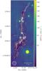 |
Fig. 1 MIPS 24 μm emission overlaid with infrared extinction contours (Kainulainen & Tan 2013) starting from AV = 25 mag and progressing inwards in steps of 20 mag. Massive dense Herschel cores from Nguyen Luong et al. (2011) are marked with white diamonds. The white dashed line indicates the peak intensity ridge of NH3 (1, 1) emission (see Sect. 2.1). The dashed gray rectangles illustrate the extent of IRAM 30 m (outer box) and PdBI (inner box) N2H+ maps (Henshaw et al. 2013, 2014), while the extent of the whole figure corresponds to the area mapped with the GBT. |
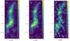 |
Fig. 2 Data products from GBT observations of G035.39. Integrated intensities of NH3 inversion transitions (1, 1) and (2, 2), (a) and (b), respectively; and integrated intensity of the rotational CCS (2–1) line (c). NH3 (2, 2) and CCS lines were integrated between 43 and 47 km s-1 to highlight the emission features, while the NH3 (1, 1) line was integrated between 20 and 70 km s-1. Extinction contours from Kainulainen & Tan (2013) at AV = 25 and 65 mag are shown in white. |
2. Observations
2.1. GBT observations
Robert C. Byrd Green Bank Telescope (GBT) observations of G035.39 were carried out on 2010 Feb. 27 and 28 (project GBT/10A-067, PI: Ke Wang). G035.39 was covered in Nyquist sampled on-the-fly (OTF) maps scanning along RA and Dec. The K-band receiver was equipped with two beams (B3 and B4) separated by 178.8 arcsec in azimuth. We used the frequency switching mode, with ±2.5 MHz switch for the two signal states, in a 12.5 MHz band with a channel width of 3.05 kHz in dual polarization mode. The band covered NH3 (1, 1) and (2, 2) inversion lines, CCS (2–1) rotational transition, and NH2D (414–404); the latter being undetected. The weather conditions at the GBT site were stable during the observing run, with pointing accuracy resulting from winds alone estimated to be below 3′′. The system temperatures were at 38–45 K during the first day and between 58 and 78 K during the second day.
To estimate the absolute flux of the observed emission, we performed nodding observations of the quasar 3C 48. For each beam, polarization, and spectral window states, the data were then reduced in GBTIDL v2.10.1 to yield main beam temperatures for each state. Using a spectral flux density model from Ott et al. (1994), we derived the predicted flux for 3C 48. When compared to reduced nodding observations, the model is consistent within 10% for ammonia spectral windows. The off-source beam B4, however, was found to be mismatched by 50–90% in integrated intensity when compared to the on-source beam, and was consequently removed from the following discussion. As the area mapped by B4 was mainly off the bulk of G035.39, the decision to drop the beam from a subsequent discussion does not affect the results of this study.
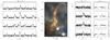 |
Fig. 3 A composite Hi-GAL color image of the infrared dark cloud. Red, green, and blue channels correspond to 350, 250, and 160 μm, respectively. To the left of the Herschel map, four NH3 (1, 1) spectra are shown, and four selected NH3 (2, 2) and CCS (2–1) lines are displayed on the right side of the central figure. The CCS spectra are smoothed to 0.12 km s-1. Each row of spectra is arranged to match the black diamond markers shown on the FIR map, selected to represent typical spectra along the filament. The filament ridge, as defined in Sect. 2.1, is marked with a dashed white line. |
The OTF observations of G035.39 were calibrated via the GBT pipeline1 (Masters et al. 2011) into main beam temperature units and imaged with the GBT Ammonia Survey (GAS, Friesen et al. 2017) pipeline2, modified to address spectral setup differences. The full width at half maximum of the GBT beam at NH3 (1, 1) line frequency (32′′) was used to set the pixel size for all spectral line cubes, at three pixels per beam. The final spectral resolution of the data is 38.6 m s-1.
2.2. Herschel public data
As mentioned in Sect. 1, the entire extent of G035.39 has been studied before with the Herschel Space Observatory (Pilbratt et al. 2010) by Nguyen Luong et al. (2011). To quantify the difference in gas- and dust-derived properties, we use the available G035.39 data from the Herschel infrared Galactic Plane Survey (Hi-GAL, Molinari et al. 2010).
The data products used in this study, photometric maps from PACS (Poglitsch et al. 2010) and SPIRE (Griffin et al. 2010) cameras, were downloaded from the image server of the first public Hi-GAL data release (DR1, Molinari et al. 2016), observation IDs 1342219631 and 1342219630. The DR1 data underwent processing by the ROMAGAL pipeline (Traficante et al. 2011), and in particular, had its absolute levels of emission calibrated. This allows us to directly put constraints on the properties of dust emission.
3. Results
3.1. Overview of the data
The integrated intensity maps for ammonia and CCS transitions observed with the GBT are presented in Fig. 2. Not accounting for the bright NH3 satellite lines, the majority of the molecular emission detected from the cloud is situated between 43 and 46 km s-1. A prominent secondary component is present in the southern region of the cloud and, furthermore, strong line asymmetries indicate the presence of additional line-of-sight components (see Fig. 3 for example spectra).
Given the low signal-to-noise ratio of the CCS (2–1) line, its kinematics cannot be easily constrained, and the transition is not discussed throughout this work. We note that the southern peak of the integrated intensity of the CCS coincides with a peak of the mid-infrared extinction map (Fig. 2c), and has no associated 24- and 70 μm point sources. As the carbon-chain molecules are known to trace regions of early-stage chemistry (Suzuki et al. 1992), the CCS peak may be indicative of dense gas in an earlier evolutionary stage than the rest of the cores in the IRDC. More dedicated studies will be carried out toward this region in the future.
As the large-scale structure of the cloud’s main velocity component manifests itself as a prominent, continuous filament, we can probe how its physical properties vary along its length. We set the line segment defining the filament from the ammonia intensity profile. The maximal value of the NH3 (1, 1) integrated intensity along right ascension is calculated for each value of declination. The longest continuous segment is then taken from the obtained set of coordinate points, with a continuity condition that the neighboring points must be in the same GBT beam. This approach, adequately simplistic for our task of probing pc-scale structure, recovers the intensity ridge of G035.39 without the need to resort to more sophisticated ridge-detection methods. The resulting filament profile is marked in Fig. 1.
In the far-infrared Herschel photometric maps, G035.39 manifests itself as a typical infrared dark cloud, characterized by its emission at longer wavelengths. It appears as an extinction feature in the 70 μm band of PACS, and as an emission feature from 160 μm onwards. The central panel in Fig. 3 displays a color-composite image of the IRDC, with 350, 250, and 160 μm emission used for red, green, and blue channels, respectively. As both ammonia and dust continuum trace the dense gas that constitutes the bulk of the cloud, the far-infrared morphology does not show any significant deviations from the NH3-defined filament ridge. A clearly visible substructure in PACS 160 μm and SPIRE 250 μm maps can be attributed to those Herschel bands having angular resolutions (12′′ and 18′′, respectively) different from our NH3 observations (32′′). The properties derived from the Herschel maps were then regridded onto the grid given by our GBT observations.
3.2. Ammonia line fitting
The ammonia molecule has been proven to be an invaluable tool in probing physical conditions of moderately dense molecular regions (e.g., Myers & Benson 1983; Rosolowsky et al. 2008; Pillai et al. 2006; Pineda et al. 2010; Wang et al. 2012, 2014), and the ratio of its collisionally populated metastable (J,K) = (1, 1) and (2, 2) inversion states can be used to derive the rotational gas temperature Trot (Ho & Townes 1983). This temperature is commonly used as a proxy value for the kinetic temperature of the medium, derived through balancing the rates of radiative and collisional transitions (Walmsley & Ungerechts 1983; Tafalla et al. 2004; Swift et al. 2005).
 |
Fig. 4 Panel a: Fitted velocities relative to line rest frequency. Overlaid on the main velocity component, additional components, enclosed in the black contours, are shown in the cut-outs. The ridge of G035.39, as defined in Sect. 2.1, is marked as a dashed black line. Panel b: Same as a, but for the fitted velocity dispersions. |
In the Rayleigh–Jeans approximation, an observed spectral profile of the two inversion lines along with their hyperfine components can be described as a sum over their hyperfines, assuming uniform excitation conditions for all the hyperfine components of the lines and a unity beam filling factor (e.g., Stahler & Palla 2005): ![Mathematical equation: \begin{equation} \label{eq:line_profile} T_{\mathrm{MB}}(v) = \sum_i\left\{1 - \mathrm{exp}\left[-r_i~\tau_0~\mathrm{exp}\left(-\frac{(\voff-v_i)^2}{2\sigma_v^2}\right)\right]\right\}(\Tex - \Tbg), \end{equation}](/articles/aa/full_html/2017/10/aa30350-16/aa30350-16-eq29.png) (1)where Tex describes the population ratios of the inversion transition parity levels, the background radiation temperature Tbg is taken to be that of the cosmic microwave background (2.7312 K), ri are normalized relative intensities of the hyperfine components, vi is the velocity centroids of the hyperfine components, σv is the velocity dispersion, and τ0 is the main group opacity of the corresponding inversion line. The latter can be used to derive the column density of the (1, 1) rotational state N(1, 1) (Rosolowsky et al. 2008):
(1)where Tex describes the population ratios of the inversion transition parity levels, the background radiation temperature Tbg is taken to be that of the cosmic microwave background (2.7312 K), ri are normalized relative intensities of the hyperfine components, vi is the velocity centroids of the hyperfine components, σv is the velocity dispersion, and τ0 is the main group opacity of the corresponding inversion line. The latter can be used to derive the column density of the (1, 1) rotational state N(1, 1) (Rosolowsky et al. 2008):  (2)and can then be scaled to a total ammonia column density Ntot via a partition function, assuming that only the metastable population levels are populated (Rosolowsky et al. 2008). The spectral profile modelling and line fitting are done following the method presented in Friesen et al. (2017), where the NH3 (1, 1) and (2, 2) spectra are simultaneously modelled using Eq. (1) within the pyspeckit (Ginsburg & Mirocha 2011) Python package. The spectral profile of both inversion lines are fitted considering the following free parameters: kinetic temperature Tkin, excitation temperature Tex, ammonia column density Ntot, velocity offset with respect to line rest frequency voff, and velocity dispersion σ.
As mentioned in Sect. 3.1, multiple line-of-sight components are present in the ammonia spectra. Their interchangeable strength and unknown a priori locations make conventional line-fitting techniques difficult to apply. In particular, the iterative nonlinear least-squares algorithm (Levenberg 1944; Marquardt 1963) used in pyspeckit is prone to failures to reach global convergence in the presence of multiple local minima. To ensure convergence of the algorithm on the global minima, we perform parameter space gridding to select initial guesses for the fitting routine. As the parameters that vary the most among our spectra are the line centroids and their peak amplitudes, we search for the optimal starting conditions by varying Tex and voff.
By inspecting the NH3 (1, 1) spectra for line peaks and line asymmetries, we have set the velocity intervals at which the line centroids could reside. The six intervals selected are centered at 42.9, 44.6, 45.5, 47.0, 55.2, and 72.2 km s-1. The velocity components that were found to overlap spatially were each split into ten values, corresponding to velocity steps of ≤0.1 km s-1. Additionally, we consider a range of 10 Tex values set up to cover the amplitude range of our NH3 (1, 1) data. The resulting velocity and line brightness ranges for component pairs that were found to overlap were then permuted together to yield over 50 k modeled spectra. Each modeled spectral profile was subsequently checked against all the pixels in our data, and the models with the lowest total squared residuals were used as a starting point for the nonlinear least squares routine. The source code for the initial guess selection method described above is freely available online3.
For every pixel of the spectral cube obtained from Sect. 2.1, we perform a multiple component nonlinear least-squares fit for one and two velocity components. To decide on a number of components present in a spectrum, one needs to rule out overfitting. As a direct minimization of the square of residuals would always prefer a more complex model, we limit the multiple component fits, requiring the best-fit solution to have a signal-to-noise ratio of at least three in all components and for those components to have a peak separation larger than the line widths of the two components. Should any of these criteria not be met, a simpler model is preferred – one velocity component for a failed double peak fit, or a spectrum is masked altogether if a single peak fit fails.
3.3. Parsec-scale kinematics of the IRDC
The structure of G035.39 can be seen as a combination of a main velocity component and additional velocity components along the line of sight. We refer to the coherent structure at 44–47 km s-1 as the main velocity component. For spectra with two identified line components, components that are brighter than their counterparts are considered to belong to the main group. In G035.39, this choice results in a spatially coherent velocity field traced by the main component.
Figure 4 illustrates the kinematics of the main velocity component, overlaid with additional identified velocity components. Of these additional components, the ones found in G035.39-N (the 44 and 46 km s-1 components) coincide with the network of filaments from Henshaw et al. (2014). Two more velocity components are identified in both ammonia transitions from the spectral cube inspection, but at 55km s-1 and 72km s-1 are unlikely to be related to the main body of the IRDC. Additionally, a strong (up to peak TMB = 1.5 K) velocity component, well-separated from the main cloud component by ~2 km s-1, is present at the location of the active star formation in the southern part of the IRDC. This is consistent with the location and vlsr of Filament 1 from Jiménez-Serra et al. (2014) at its southernmost point.
The velocity of the main ammonia component gradually changes from red- to blue-shifted in the southward direction. Figure 5 illustrates this change, showing the velocity centroid and velocity dispersion profiles along the IRDC intensity ridge. The non-thermal velocity dispersions of ammonia (Myers 1983) have a large dynamic range, sometimes going as high as 1.2 km s-1 at the edges of the map, but generally staying within the interquartile range between 0.38 and 0.52 km s-1 (Fig. 5b). These high values, implying non-thermal motions dominating the line width, are above those found in low-mass cores and are in the upper range of typical non-thermal components of massive cores (Caselli & Myers 1995). For the H2 sound speed derived from the fitted ammonia kinetic temperatures and assuming a mean mass per particle of 2.33 u, the average Mach number across the IRDC is ℳ = 2.14, consistent with previous studies of G035.39 that find gas motions in the cloud to be supersonic (Henshaw et al. 2014; Jiménez-Serra et al. 2014).
The gradual change of the line centroid towards the southern portion of the IRDC can be quantified in terms of a velocity gradient. Previous studies of G035.39 have discussed the global gas motions on various scales. Henshaw et al. (2014) attribute radial velocity irregularity towards the northern part of G035.39-N found by Henshaw et al. (2013) to the unresolved substructure, and find the global gradients in identified filaments to be smaller than 0.7 km s-1 pc-1. Jiménez-Serra et al. (2014) find global, north-south velocity gradients of ~ 0.4 − 0.8km s-1 pc-1 along three CO filaments in G035.39. As our GBT data covers the full extent of the cloud, we are able to constrain the global velocity gradient along the whole IRDC. A least squares fit to the ridge velocity profile, weighted by uncertainties in centroid velocities, results in a line-of-sight velocity gradient of ∇v ~ 0.2km s-1 pc-1 along the filament’s 6 pc length (Fig. 5a). This value is in good agreement with the average velocity gradients reported for larger-scale filament and GMC structures (e.g., Hernandez & Tan 2015; Wang et al. 2016).
While the global velocity gradient following the ridge of G035.39 is well described on scales larger than one parsec, smaller-scale, oscillatory-like deviations from the fitted linear relation are present. Additionally, hints of a localized third component towards the southern 42.6 km s-1 feature are manifested as a broader velocity dispersion at the edge of G035.39 (see Fig. 6 for an example fit with irregular residual); as it is mostly blended with the main component, constraining its properties is difficult due to the limited angular resolution of the GBT data. Ammonia emission is often highly substructured in star-forming regions, and can manifest itself as filamentary emission down to ~ 5000 AU scales (Pineda et al. 2011, 2015). The exact nature of the velocity substructure in the southern part of G035.39 can be seen as either stemming from the coherent gas motions around the dense cores (e.g., Hacar & Tafalla 2011; Zhang et al. 2015; Gritschneder et al. 2017), or as a picture reminiscent of the nearby low-mass star forming Taurus complex, where previously unresolved velocity-coherent filaments are found to be bundled together in a larger structure (Hacar et al. 2013; Tafalla & Hacar 2015). The velocity irregularities along the cloud may result from the sub-pc substructure emission (similar to the already resolved one in the G035.39-N region by Henshaw et al. 2014), being smoothed by the GBT beam. The higher angular resolution analysis of the gas kinematics along the entire IRDC will be addressed in a future study.
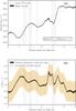 |
Fig. 5 Panel a: The radial velocity profile of the main component along the G035.39 filament, starting at its southernmost point. The solid black line shows the radial velocities fit at the intensity ridge of the IRDC. The width of the solid black line represents the fitting uncertainty at each point. The vertical dotted lines mark the projected locations of the massive protostellar cores from Nguyen Luong et al. (2011). Panel b: Same as a, but for the velocity dispersion profile along the IRDC ridge. The yellow shaded region denotes the spread area given by two standard deviations of all σ values in the main velocity component. |
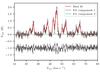 |
Fig. 6 NH3 (1, 1) spectrum towards α(J2000) = 18h57m10.1s and δ(J2000) = +2°08′23′′, overlaid with the best two-component fit model. A significant residual, revealing the presence of the unconstrained third component, is plotted alongside the spectrum, offset by 1 K. The spectrum was smoothed to 0.08 km s-1 for visual clarity. |
3.4. Gas temperature
While the profile of the NH3 (1, 1) line can be constrained accurately in the pixels with significant emission, the (2, 2) line is considerably weaker in the low-temperature regime. Because of this, we impose a more stringent constraint on the physical parameters that depend primarily on the (2, 2) inversion transition – namely, kinetic temperature and total ammonia column density. For these, we only select spectra that have >3σI detection in the integrated intensity. We take the expression for integrated intensity uncertainty,  , from Mangum & Shirley (2015), where N is the number of channels with nonzero emission in a modeled spectrum (arbitrarily taken to be 10-5 K), σTMB is the corresponding TMB uncertainty, and Δvc is the channel width in the GBT spectra.
The gas kinetic temperature of the main component of G035.39 is presented in Fig. 7. The derived values vary across the body of the dark cloud from about 11 K to 15 K. The cold gas temperature range is typical of other IRDCs (Pillai et al. 2006; Ragan et al. 2012; Chira et al. 2013; Wang et al. 2012, 2014) as well as of relatively nearby low-mass starless cores (Rosolowsky et al. 2008; Friesen et al. 2009; Forbrich et al. 2014).
Due to a more stringent masking of the temperatures derived from our multi-component fit, only a handful of spectra have their kinetic temperature constrained for weaker secondary components. As most of the derived values of the gas kinetic temperature belong to the main component, the discussion on the temperature of the weaker components is thus effectively restricted to those few detections. In the star-forming part of G035.39-N, towards the northern group of the star-forming cores, we successfully measure the gas temperature for two components along the line of sight to be between 12.9 and 13.3 K.
The region coincident with a bright infrared source south-east of the main filament (55 km s-1 cut-out in Fig. 4) is consistently hotter than the bulk of the IRDC. The derived temperatures for the gas associated with the source range from 17.5 to 20.9 K, suggesting that the gas is internally heated. Nguyen Luong et al. (2011) identify the source as an infrared-bright protostellar MDC, and derive its dust temperature to be 26 ± 6 K. As the ammonia emission for this component is peaked at 55 km s-1, it appears to be physically unrelated to G035.39. Similarly, for a spectral line detected at 72 km s-1 (Fig. 4), which appears as a starless infrared extinction feature east of the filament, we report a kinetic temperature of 16.5 ± 1.3 K. Although defined as part of the IRDC extent in Nguyen Luong et al. (2011) based on the common column density contour, we suggest that the feature does not form a coherent structure with G035.39.
 |
Fig. 7 Kinetic temperature map derived from the main velocity component of NH3. The contour lines and diamond markers are the same as in Fig. 1. |
3.5. Dust temperature
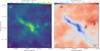 |
Fig. 8 H2 column density (a) and dust temperature (b) maps derived from Herschel data for G035.39. A 1 pc length scale and a combined Herschel beam size are shown for each map. The ammonia intensity ridge and the positions of Herschel MDCs are shown as a black dashed line and gray diamond markers, respectively. |
The intensity of an optically thin source of temperature T is given by the radiative transfer equation (e.g., Rybicki & Lightman 1979), which can be approximated by  (3)where Bν(T) is the Planck blackbody function. In the expression above, a frequency dependent opacity τν can be shown to be related to the gas column density NH2 in the following way:
  (4)where μH2 = 2.8 is the molecular weight per hydrogen molecule (Kauffmann et al. 2008), κν is the dust opacity, and mH is the mass of a hydrogen atom. For consistency with Nguyen Luong et al. (2011), we have adopted the dust opacity law of κν ∝ νβ, assuming a gas-to-dust mass ratio of 100 from Hildebrand (1983). As the optically thin approximation in Eq. (3) does not necessarily hold for PACS bands at high column densities, we discuss its limitations for the PACS data. While the 160 μm PACS band is expected to be within the optically thin approximation well into the high density regime (τ160 = 0.16 for NH2 = 1023 cm-2), the 70 μm maps may trace extinction of dust rather than its emission (G035.39 appears as an extinction feature in 70 μm), rendering the optically thin dust emission assumption invalid (e.g., Battersby et al. 2011).
Hi-GAL PACS and SPIRE maps containing G035.39 were jointly convolved to a common resolution of 34.5′′, corresponding to the beam size of the 500 μm SPIRE band. The maps were then regridded to 11.5′′ pixel size to form spectral cubes. The resulting cube was fit pixel-by-pixel with a single temperature gray-body model described above, assuming a fixed value of β = 2 (e.g., Stutz et al. 2010; Nguyen Luong et al. 2011; Elia et al. 2013; Lombardi et al. 2014). Fixing the value of β reduces the number of free parameters for an otherwise degenerate model (e.g., Planck Collaboration XXV 2011; Kelly et al. 2012). While implicit assumptions on the spectral opacity index are made in such a way, it enables an estimation of the resulting parameter uncertainties by minimizing the errors stemming from the model degeneracy. In the above analysis, we have considered 30% uncertainty on the flux levels for consistency with Nguyen Luong et al. (2011).
Column density and effective dust temperature maps, derived for the Herschel regions from 160, 250, 350 and 500 μm Herschel bands, are presented in Fig. 8. The column density and dust temperature values show anti-correlation, typical for externally irradiated clouds (Evans et al.2001; see also Planck Collaboration XXV2011), and IRDCs (e.g., Wang et al. 2015, Appendix). The overall morphology of the density and temperature structure in the derived parameter maps is similar to that of Nguyen Luong et al. (2011).
3.6. Molecular abundances
The column densities from Herschel and those of ammonia correlate weakly (r = 0.64, Fig. 9), and show no evidence for ammonia depletion, consistent with previous work toward nearby starless cores (Tafalla et al. 2002). By taking the ratio of the two we derive the ammonia abundance in G035.39, X(NH3) = [ N(NH3) /N(H2) ]. The mean value of the total NH3 abundance is ~ 2.1 × 10⁻⁸, corresponding to the para-NH3 abundances of ~ 1.0 × 10⁻⁸ assuming the ortho- to para-NH3 ratio of one. The range of abundances is comparable to that found towards the centers of low-mass cores (Tafalla et al. 2004; Crapsi et al. 2007; Friesen et al. 2017), and is in good agreement with values measured towards the low-mass star-forming cluster Serpens South (Friesen et al. 2016). When compared to other IRDCs, our GBT data on G035.39 point to lower abundances – Ragan et al. (2011) derive NH3 abundances of a few times 10-7. However, Ragan et al. observe their IRDC sample with much smaller beam size of the VLA, therefore allowing for a small beam filling factor of our observations may mitigate the discrepancy. Indeed, for an angular resolution of 40′′ and a median sample distance of 2.9 kpc, Pillai et al. (2006) report X(NH3) as being between 7 × 10⁻⁹ and 10-7, consistent with our findings.
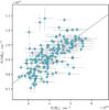 |
Fig. 9 Herschel-derived H2 gas column density plotted against fitted NH3 column density. The dashed straight line passes through both the mean ammonia abundance in the IRDC and through the zero column density point. |
4. Discussion
4.1. A comparison of dust and gas temperatures
Current understanding of heating and cooling processes within dense molecular clouds requires close coupling between gas and dust at number densities above ~ 105 cm-3 (Goldsmith 2001). However, no correlation of dust and gas temperatures is found in G035.39 (Pearson’s r = − 0.16), despite the uncertainties on the temperatures being significantly smaller than the temperature dynamical range. Moreover, the dust temperatures derived from Herschel are consistently higher than the ammonia-based gas temperatures, suggesting that the two sets of observations are sensitive to different environments. Dust temperatures higher than the gas temperatures have previously been reported. Forbrich et al. (2014) find dust temperatures to be 2–3 K warmer than the gas temperatures towards starless cores in the Pipe nebula. More recently, Friesen et al. (2016) report their ammonia-derived kinetic gas temperatures to be consistently lower than their Herschel counterparts. The difference in the two temperature tracers can be attributed to the line-of-sight mixing of warm foreground dust emission into the far-infrared SED, thus raising the effective line-of-sight average dust temperature. Ammonia gas temperature, on the other hand, is expected to trace the dense inner region of the filament only.
While the Herschel dust temperature map does not show any signs of local enhancements in the vicinity of dense cores, our NH3 results point to local temperature increases of about 1 K toward the sites of active star formation. The magnitude of the effect is comparable to what Foster et al. (2009) find towards Perseus, where protostellar cores have been found to have ammonia-derived kinetic temperatures 1.3 K larger than the starless cores. To further investigate the possibility of dense gas heated by embedded protostars, we split the pixels into two groups: those within one GBT beam from the massive dense cores in Nguyen Luong et al. (2011) and those outside of it. A number of cores with masses lower than 20 M⊙ were identified by Nguyen Luong et al. (2011) in addition to MDCs. As the total luminosity output of those cores is, on average, half of that of the MDCs, we restrict the spatial temperature distribution analysis to distance from the MDCs only. We find the median values of the gas kinetic temperatures to be 13.1 K inside the one beam radii, and 12.5 K outside of them. On the contrary, the median dust temperature increases from 15.9 to more than 18 K away from the massive dense cores (Fig. 8). In order to visualize the opposite trends in gas and dust temperatures, we plot their kernel density estimations as a function of distance to the closest massive Herschel core (Fig. 10a). The contours in Fig. 10 represent the levels of the density function based on the scatter of the temperature points only, as the fitting uncertainties in both ammonia- and dust-based temperatures are much smaller than the dynamic range of the trends in figure. The mean temperature errors and their standard deviations are σTkin = 0.38 ± 0.15 K and σTdust = 0.36 ± 0.09 K for gas and Herschel dust temperatures, respectively.
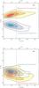 |
Fig. 10 Panel a: Fitted temperatures as a function of distance from the closest massive dense core. The contour overlays show varying levels of kernel density estimation of dust (in red) and gas (in blue) temperatures. The contour σ-levels are equivalent to that of a bivariate normal distribution, starting at 0.5σ and progressing outwards in steps of 0.5σ. The vertical dashed line indicates the beam size of the GBT. Panel b: Same as panel a, but for the dust temperatures derived via the Galactic Gaussian (GG) method. |
Systematically different values of dust and gas temperatures stress the importance of considering the line of sight mixing of the IRDC component with the warm dust emission. A number of methods for estimating the background component in Herschel photometric data are available (e.g., Wang et al. 2015)4. To address the line of sight contamination effects on the dust temperatures, we model the line of sight contamination of dust emission via two approaches:
-
A Galactic Gaussian method (GG, Battersbyet al. 2011), assum-ing that the Galactic contribution follows a Gaus-sian profile along the latitude direction within− 1deg ≤ b ≤ + 1deg latitude interval.
-
A Small Median Filter method (SMF), which interpolates the background contribution from the region outside a predefined IRDC boundary (Simon et al. 2006; Butler & Tan 2009) and estimates the 160 to 500 μm foreground by utilizing the SED model of diffuse ISM (Draine & Li 2007) normalized to the available 24 μm extinction data (Lim & Tan 2014; Lim et al. 2015).
A detailed description of each method is presented in Lim et al. (2016). The GG- and SMF-processed Herschel maps were used to derive the corrected column density and dust temperature maps following Sect. 3.5.
We find that both subtraction methods result in lower dust temperatures in G035.39, with the average values for the GG and SMF dust temperatures being 12.4 ± 1.0 and 13.8 ± 0.9 K, respectively. These values, compared to the mean gas kinetic temperature Tkin = 12.9 ± 0.8 K, suggest that the corrections applied to the Herschel maps shifted the peak of the dust SEDs into the temperature regime that much better reflects the actual gas temperature. Figure 10b shows the same distance-temperature relation as Fig. 10a, but for the GG method, a method that matches the ammonia temperature trend the closest. Despite the two trends showing some degree of agreement, no significant correlation is found between the two temperatures (Pearson’s r = 0.26).
4.2. Stability of the filament
The support of a filament against the gravitational collapse is often discussed in terms of its mass to length ratio, or line mass (M/L). We estimate the line mass from the Hi-GAL H2 column density map on the pixels that have ammonia detection. The total mass can be estimated as a sum over the column density pixels as follows: 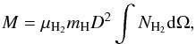 where D = 2.9 kpc is a kinematic distance to G035.39.
The mass estimate above is representing a sum over all optically thin dust emission, including both the physical region traced by the GBT ammonia observations and a contribution along the line of sight. To subtract line of sight contamination, we make a simplistic assumption that the total gas column of this extra LoS material is equal to a mean NH2 value along the bounding contour around the NH3 (2, 2) detection of the main velocity component. We apply a correction offset of 2.64 × 1022 cm-2 to the G035.39 gas column density map. By summing over the column densities within the bounding contour, we find the mass of G035.39 to be 1218M⊙, corresponding to (M / L) ≈ 223M⊙ pc-1. We argue that this value, limited both by the sensitivity-limited (2, 2) detection and the column density correction above, should resemble a lower limit to the line mass of the filament. A similarly derived (M/L) value for the (1, 1) detection yields a line mass of 319M⊙ pc-1, while the mass to length ratio of the filament without the envelope subtraction is 634M⊙ pc-1. Similarly, if the GG and SMF-derived densities are used to calculate the line mass as above, we obtain (M/L) values of 635 and 494M⊙ pc-1, respectively, for slightly different values of Tdust. The representative range of line mass values, 223–635 M⊙ pc-1, is an order of magnitude higher than the critical line mass of thermally supported filament at 15 K, highlighting the importance of other means of support, such as non-thermal motions or magnetic fields.
Given our ammonia fitting results, we can calculate what critical line mass would be needed for the filament to be in equilibrium. By adapting the conventional filamentary virial analysis (Chandrasekhar & Fermi 1953; Ostriker 1964) to include both thermal and non-thermal support (Fiege & Pudritz 2000) one can estimate the critical line mass to be 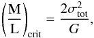 where
where  is a quadrature sum of the non-thermal velocity dispersion σnt and the isothermal sound speed cs. The range of non-thermal motions representative of the filament points to the critical line masses from 50 to 200 M⊙ pc-1, consistently lower than the Herschel-derived (M/L) range. Similarly, this critical line mass value regime is lower than the (M / L)crit values derived from the CO emission (470–1070 M⊙ pc-1, Hernandez & Tan 2011; Hernandez et al. 2012). This apparent disparity may result from the bulk of ammonia emission being more sensitive to the inner filament material of G035.39 than the CO data, as the former is known to be relatively enhanced in the denser regions of starless cores (Tafalla et al. 2002), where the CO is frozen-out onto dust grains. This proposition is supported by PdBI observations of continuum structures with much smaller spatial scales (0.03–0.07 pc), where Henshaw et al. (2016) suggest that magnetic fields are playing an important role against gravitational collapse of compact continuum cores. We suggest that their conclusions on the dynamical state of compact dense cores may be extended to the larger-scale ammonia filament in this study.
5. Conclusions
IRDC G035.39–00.33 was studied in its entirety with the Green Bank Telescope. The morphology of the cloud at this resolution resembles that of a smooth filament, more than six parsec in projected length. Multiple distinct components are present along the line of sight throughout the length of the cloud.
-
1.
We derive a reliable map of the gas temperature for the entireG035.39 cloud. The extended gas reservoir in the IRDC isconsistent with being of starless nature (Tkin ~ 11–15 K). We find evidence of gas heating from the embedded protostars, manifested as slight temperature increase around the positions of 70 μm sources.
-
2.
Despite having a similar angular resolution, the Herschel observations point to temperatures 2–3 K higher than that of the GBT observations, which can be attributed to the effects of line-of-sight contamination. We show that this offset can largely be mitigated by accounting for the background and foreground emission components. Reliance on the dust temperature maps derived from conventional FIR SED fitting with no accounting for the line of sight contributions may consistently overestimate the temperature of the dense gas.
-
3.
We find the brightest velocity component of G035.39 to exhibit a smooth, consistent velocity gradient of ~ 0.2km s-1 pc-1 magnitude. This velocity gradient is much lower than that found on smaller scales towards G035.39-N, but is consistent with the global gas motions on parsec and GMC scales.
-
4.
Additionally to the large-scale gradient across the filament, local velocity field irregularities point to the presence of substructure and smaller-scale fragmentation at scales not traced by the GBT. We suggest that an intertwined network of compact filaments might exist in the southern part of the IRDC, possibly continuing from the one found in G035.39-N. Higher-angular-resolution observations are needed to fully resolve the sub-structured kinematics of the cloud.
Acknowledgments
We would like to thank the anonymous referee for their comments which helped to improve this manuscript. The Green Bank Observatory is a facility of the National Science Foundation operated under cooperative agreement with Associated Universities, Inc. V.S., J.E.P., and P.C. acknowledge the support from the European Research Council (ERC; project PALs 320620). K.W. is supported by grant WA3628-1/1 of the German Research Foundation (DFG) through the priority program 1573 (“Physics of the Interstellar Medium”). I.J.-S. acknowledges the financial support received from the STFC through an Ernest Rutherford Fellowship (proposal number ST/L004801/2). J.C.T. acknowledges NASA grant 14-ADAP14-0135. This research made use of Astropy, a community-developed core Python package for Astronomy (Astropy Collaboration et al. 2013), and of APLpy, an open-source plotting package for Python (Robitaille & Bressert 2012). In addition, this work made use of the dust_emissivity package5 in the derivation of Herschel dust properties.
References
- André, P., Men’shchikov, A., Bontemps, S., et al. 2010, A&A, 518, L102 [NASA ADS] [CrossRef] [EDP Sciences] [Google Scholar]
- Astropy Collaboration,Robitaille, T. P., Tollerud, E. J., et al. 2013, A&A, 558, A33 [NASA ADS] [CrossRef] [EDP Sciences] [Google Scholar]
- Barnes, A. T., Kong, S., Tan, J. C., et al. 2016, MNRAS, 458, 1990 [NASA ADS] [CrossRef] [Google Scholar]
- Battersby, C., Bally, J., Ginsburg, A., et al. 2011, A&A, 535, A128 [NASA ADS] [CrossRef] [EDP Sciences] [Google Scholar]
- Beuther, H., & Shepherd, D. 2005, in Cores to Clusters: Star Formation with Next Generation Telescopes, eds. M. S. N. Kumar, M. Tafalla, & P. Caselli, Astrophys. Space Sci. Lib., 105 [Google Scholar]
- Butler, M. J., & Tan, J. C. 2009, ApJ, 696, 484 [NASA ADS] [CrossRef] [Google Scholar]
- Butler, M. J., & Tan, J. C. 2012, ApJ, 754, 5 [NASA ADS] [CrossRef] [Google Scholar]
- Caselli, P., & Myers, P. C. 1995, ApJ, 446, 665 [NASA ADS] [CrossRef] [Google Scholar]
- Chambers, E. T., Jackson, J. M., Rathborne, J. M., & Simon, R. 2009, ApJS, 181, 360 [NASA ADS] [CrossRef] [Google Scholar]
- Chandrasekhar, S., & Fermi, E. 1953, ApJ, 118, 116 [NASA ADS] [CrossRef] [MathSciNet] [Google Scholar]
- Chira, R.-A., Beuther, H., Linz, H., et al. 2013, A&A, 552, A40 [NASA ADS] [CrossRef] [EDP Sciences] [Google Scholar]
- Crapsi, A., Caselli, P., Walmsley, M. C., & Tafalla, M. 2007, A&A, 470, 221 [NASA ADS] [CrossRef] [EDP Sciences] [Google Scholar]
- Draine, B. T., & Li, A. 2007, ApJ, 657, 810 [NASA ADS] [CrossRef] [Google Scholar]
- Egan, M. P., Shipman, R. F., Price, S. D., et al. 1998, ApJ, 494, L199 [NASA ADS] [CrossRef] [Google Scholar]
- Elia, D., Molinari, S., Fukui, Y., et al. 2013, ApJ, 772, 45 [NASA ADS] [CrossRef] [Google Scholar]
- Evans, II, N. J., Rawlings, J. M. C., Shirley, Y. L., & Mundy, L. G. 2001, ApJ, 557, 193 [NASA ADS] [CrossRef] [Google Scholar]
- Fiege, J. D., & Pudritz, R. E. 2000, MNRAS, 311, 85 [NASA ADS] [CrossRef] [Google Scholar]
- Forbrich, J., Öberg, K., Lada, C. J., et al. 2014, A&A, 568, A27 [NASA ADS] [CrossRef] [EDP Sciences] [Google Scholar]
- Foster, J. B., Rosolowsky, E. W., Kauffmann, J., et al. 2009, ApJ, 696, 298 [NASA ADS] [CrossRef] [Google Scholar]
- Friesen, R. K., Di Francesco, J., Shirley, Y. L., & Myers, P. C. 2009, ApJ, 697, 1457 [NASA ADS] [CrossRef] [Google Scholar]
- Friesen, R. K., Bourke, T. L., Di Francesco, J., Gutermuth, R., & Myers, P. C. 2016, ApJ, 833, 204 [NASA ADS] [CrossRef] [Google Scholar]
- Friesen, R. K., Pineda, J. E., Rosolowsky, E., et al. 2017, ApJ, 843, 63 [NASA ADS] [CrossRef] [Google Scholar]
- Ginsburg, A., & Mirocha, J. 2011, PySpecKit: Python Spectroscopic Toolkit, Astrophysics Source Code Library [record ascl:1109.001] [Google Scholar]
- Goldsmith, P. F. 2001, ApJ, 557, 736 [NASA ADS] [CrossRef] [MathSciNet] [Google Scholar]
- Griffin, M. J., Abergel, A., Abreu, A., et al. 2010, A&A, 518, L3 [Google Scholar]
- Gritschneder, M., Heigl, S., & Burkert, A. 2017, ApJ, 834, 202 [NASA ADS] [CrossRef] [Google Scholar]
- Hacar, A., & Tafalla, M. 2011, A&A, 533, A34 [NASA ADS] [CrossRef] [EDP Sciences] [Google Scholar]
- Hacar, A., Tafalla, M., Kauffmann, J., & Kovács, A. 2013, A&A, 554, A55 [NASA ADS] [CrossRef] [EDP Sciences] [Google Scholar]
- Henshaw, J. D., Caselli, P., Fontani, F., et al. 2013, MNRAS, 428, 3425 [NASA ADS] [CrossRef] [Google Scholar]
- Henshaw, J. D., Caselli, P., Fontani, F., Jiménez-Serra, I., & Tan, J. C. 2014, MNRAS, 440, 2860 [NASA ADS] [CrossRef] [Google Scholar]
- Henshaw, J. D., Caselli, P., Fontani, F., et al. 2016, MNRAS, 463, 146 [NASA ADS] [CrossRef] [Google Scholar]
- Henshaw, J. D., Jiménez-Serra, I., Longmore, S. N., et al. 2017, MNRAS, 464, L31 [NASA ADS] [CrossRef] [Google Scholar]
- Hernandez, A. K., & Tan, J. C. 2011, ApJ, 730, 44 [NASA ADS] [CrossRef] [Google Scholar]
- Hernandez, A. K., & Tan, J. C. 2015, ApJ, 809, 154 [NASA ADS] [CrossRef] [Google Scholar]
- Hernandez, A. K., Tan, J. C., Caselli, P., et al. 2011, ApJ, 738, 11 [NASA ADS] [CrossRef] [Google Scholar]
- Hernandez, A. K., Tan, J. C., Kainulainen, J., et al. 2012, ApJ, 756, L13 [NASA ADS] [CrossRef] [Google Scholar]
- Hildebrand, R. H. 1983, Quant. J. Roy. Astron. Soc., 24, 267 [Google Scholar]
- Ho, P. T. P., & Townes, C. H. 1983, ARA&A, 21, 239 [NASA ADS] [CrossRef] [Google Scholar]
- Jiménez-Serra, I., Caselli, P., Tan, J. C., et al. 2010, MNRAS, 406, 187 [NASA ADS] [CrossRef] [Google Scholar]
- Jiménez-Serra, I., Caselli, P., Fontani, F., et al. 2014, MNRAS, 439, 1996 [NASA ADS] [CrossRef] [Google Scholar]
- Kainulainen, J., & Tan, J. C. 2013, A&A, 549, A53 [NASA ADS] [CrossRef] [EDP Sciences] [Google Scholar]
- Kauffmann, J., Bertoldi, F., Bourke, T. L., Evans, II, N. J., & Lee, C. W. 2008, A&A, 487, 993 [NASA ADS] [CrossRef] [EDP Sciences] [Google Scholar]
- Kelly, B. C., Shetty, R., Stutz, A. M., et al. 2012, ApJ, 752, 55 [NASA ADS] [CrossRef] [Google Scholar]
- Levenberg, K. 1944, QJRAS, II, 164 [Google Scholar]
- Lim, W., & Tan, J. C. 2014, ApJ, 780, L29 [NASA ADS] [CrossRef] [Google Scholar]
- Lim, W., Carey, S. J., & Tan, J. C. 2015, ApJ, 814, 28 [NASA ADS] [CrossRef] [Google Scholar]
- Lim, W., Tan, J. C., Kainulainen, J., Ma, B., & Butler, M. J. 2016, ApJ, 829, L19 [NASA ADS] [CrossRef] [Google Scholar]
- Lombardi, M., Bouy, H., Alves, J., & Lada, C. J. 2014, A&A, 566, A45 [NASA ADS] [CrossRef] [EDP Sciences] [Google Scholar]
- Mangum, J. G., & Shirley, Y. L. 2015, PASP, 127, 266 [NASA ADS] [CrossRef] [Google Scholar]
- Marquardt, D. W. 1963, J. Soc. Indust. Appl. Math., 11, 431 [Google Scholar]
- Masters, J., Garwood, B., Langston, G., & Shelton, A. 2011, in Astronomical Data Analysis Software and Systems XX, eds. I. N. Evans, A. Accomazzi, D. J. Mink, & A. H. Rots, ASP Conf. Ser., 442, 127 [Google Scholar]
- McKee, C. F., & Ostriker, E. C. 2007, ARA&A, 45, 565 [NASA ADS] [CrossRef] [Google Scholar]
- Molinari, S., Swinyard, B., Bally, J., et al. 2010, PASP, 122, 314 [NASA ADS] [CrossRef] [Google Scholar]
- Molinari, S., Schisano, E., Elia, D., et al. 2016, A&A, 591, A149 [NASA ADS] [CrossRef] [EDP Sciences] [Google Scholar]
- Myers, P. C. 1983, ApJ, 270, 105 [NASA ADS] [CrossRef] [Google Scholar]
- Myers, P. C., & Benson, P. J. 1983, ApJ, 266, 309 [NASA ADS] [CrossRef] [Google Scholar]
- Nguyen Luong, Q., Motte, F., Hennemann, M., et al. 2011, A&A, 535, A76 [NASA ADS] [CrossRef] [EDP Sciences] [Google Scholar]
- Ostriker, J. 1964, ApJ, 140, 1056 [NASA ADS] [CrossRef] [MathSciNet] [Google Scholar]
- Ott, M., Witzel, A., Quirrenbach, A., et al. 1994, A&A, 284, 331 [NASA ADS] [Google Scholar]
- Perault, M., Omont, A., Simon, G., et al. 1996, A&A, 315, L165 [NASA ADS] [Google Scholar]
- Pilbratt, G. L., Riedinger, J. R., Passvogel, T., et al. 2010, A&A, 518, L1 [CrossRef] [EDP Sciences] [Google Scholar]
- Pillai, T., Wyrowski, F., Carey, S. J., & Menten, K. M. 2006, A&A, 450, 569 [NASA ADS] [CrossRef] [EDP Sciences] [Google Scholar]
- Pineda, J. E., Goodman, A. A., Arce, H. G., et al. 2010, ApJ, 712, L116 [NASA ADS] [CrossRef] [Google Scholar]
- Pineda, J. E., Goodman, A. A., Arce, H. G., et al. 2011, ApJ, 739, L2 [NASA ADS] [CrossRef] [Google Scholar]
- Pineda, J. E., Offner, S. S. R., Parker, R. J., et al. 2015, Nature, 518, 213 [NASA ADS] [CrossRef] [Google Scholar]
- Planck Collaboration XXV. 2011, A&A, 536, A25 [NASA ADS] [CrossRef] [EDP Sciences] [Google Scholar]
- Poglitsch, A., Waelkens, C., Geis, N., et al. 2010, A&A, 518, L2 [NASA ADS] [CrossRef] [EDP Sciences] [Google Scholar]
- Ragan, S. E., Bergin, E. A., & Wilner, D. 2011, ApJ, 736, 163 [NASA ADS] [CrossRef] [Google Scholar]
- Ragan, S. E., Heitsch, F., Bergin, E. A., & Wilner, D. 2012, ApJ, 746, 174 [NASA ADS] [CrossRef] [Google Scholar]
- Rathborne, J. M., Jackson, J. M., & Simon, R. 2006, ApJ, 641, 389 [NASA ADS] [CrossRef] [Google Scholar]
- Robitaille, T., & Bressert, E. 2012, APLpy: Astronomical Plotting Library in Python, Astrophysics Source Code Library [record ascl:1208.017] [Google Scholar]
- Rosolowsky, E. W., Pineda, J. E., Foster, J. B., et al. 2008, ApJS, 175, 509 [NASA ADS] [CrossRef] [Google Scholar]
- Rybicki, G. B., & Lightman, A. P. 1979, Radiative processes in astrophysics (New York: Wiley-Interscience), 393 [Google Scholar]
- Sanhueza, P., Jackson, J. M., Foster, J. B., et al. 2012, ApJ, 756, 60 [NASA ADS] [CrossRef] [Google Scholar]
- Schneider, N., Csengeri, T., Klessen, R. S., et al. 2015, A&A, 578, A29 [NASA ADS] [CrossRef] [EDP Sciences] [Google Scholar]
- Simon, R., Rathborne, J. M., Shah, R. Y., Jackson, J. M., & Chambers, E. T. 2006, ApJ, 653, 1325 [NASA ADS] [CrossRef] [Google Scholar]
- Stahler, S. W., & Palla, F. 2005, The Formation of Stars (Wiley-VCH) [Google Scholar]
- Stutz, A., Launhardt, R., Linz, H., et al. 2010, A&A, 518, L87 [NASA ADS] [CrossRef] [EDP Sciences] [Google Scholar]
- Suzuki, H., Yamamoto, S., Ohishi, M., et al. 1992, ApJ, 392, 551 [NASA ADS] [CrossRef] [Google Scholar]
- Swift, J. J., Welch, W. J., & Di Francesco, J. 2005, ApJ, 620, 823 [NASA ADS] [CrossRef] [Google Scholar]
- Tafalla, M., & Hacar, A. 2015, A&A, 574, A104 [NASA ADS] [CrossRef] [EDP Sciences] [Google Scholar]
- Tafalla, M., Myers, P. C., Caselli, P., Walmsley, C. M., & Comito, C. 2002, ApJ, 569, 815 [NASA ADS] [CrossRef] [Google Scholar]
- Tafalla, M., Myers, P. C., Caselli, P., & Walmsley, C. M. 2004, A&A, 416, 191 [NASA ADS] [CrossRef] [EDP Sciences] [Google Scholar]
- Tan, J. C., Kong, S., Butler, M. J., Caselli, P., & Fontani, F. 2013, ApJ, 779, 96 [NASA ADS] [CrossRef] [Google Scholar]
- Tan, J. C., Beltrán, M. T., Caselli, P., et al. 2014, Protostars and Planets VI (Wiley-VCH), 149 [Google Scholar]
- Traficante, A., Calzoletti, L., Veneziani, M., et al. 2011, MNRAS, 416, 2932 [NASA ADS] [CrossRef] [Google Scholar]
- Walmsley, C. M., & Ungerechts, H. 1983, A&A, 122, 164 [NASA ADS] [Google Scholar]
- Wang, K., Zhang, Q., Wu, Y., & Zhang, H. 2011, ApJ, 735, 64 [NASA ADS] [CrossRef] [Google Scholar]
- Wang, K., Zhang, Q., Wu, Y., Li, H.-B., & Zhang, H. 2012, ApJ, 745, L30 [NASA ADS] [CrossRef] [Google Scholar]
- Wang, K., Zhang, Q., Testi, L., et al. 2014, MNRAS, 439, 3275 [NASA ADS] [CrossRef] [Google Scholar]
- Wang, K., Testi, L., Ginsburg, A., et al. 2015, MNRAS, 450, 4043 [NASA ADS] [CrossRef] [MathSciNet] [Google Scholar]
- Wang, K., Testi, L., Burkert, A., et al. 2016, ApJS, 226, 9 [NASA ADS] [CrossRef] [Google Scholar]
- Zhang, Q., Wang, K., Lu, X., & Jiménez-Serra, I. 2015, ApJ, 804, 141 [NASA ADS] [CrossRef] [Google Scholar]
All Figures
|
Fig. 1 MIPS 24 μm emission overlaid with infrared extinction contours (Kainulainen & Tan 2013) starting from AV = 25 mag and progressing inwards in steps of 20 mag. Massive dense Herschel cores from Nguyen Luong et al. (2011) are marked with white diamonds. The white dashed line indicates the peak intensity ridge of NH3 (1, 1) emission (see Sect. 2.1). The dashed gray rectangles illustrate the extent of IRAM 30 m (outer box) and PdBI (inner box) N2H+ maps (Henshaw et al. 2013, 2014), while the extent of the whole figure corresponds to the area mapped with the GBT. |
| In the text | |
|
Fig. 2 Data products from GBT observations of G035.39. Integrated intensities of NH3 inversion transitions (1, 1) and (2, 2), (a) and (b), respectively; and integrated intensity of the rotational CCS (2–1) line (c). NH3 (2, 2) and CCS lines were integrated between 43 and 47 km s-1 to highlight the emission features, while the NH3 (1, 1) line was integrated between 20 and 70 km s-1. Extinction contours from Kainulainen & Tan (2013) at AV = 25 and 65 mag are shown in white. |
| In the text | |
|
Fig. 3 A composite Hi-GAL color image of the infrared dark cloud. Red, green, and blue channels correspond to 350, 250, and 160 μm, respectively. To the left of the Herschel map, four NH3 (1, 1) spectra are shown, and four selected NH3 (2, 2) and CCS (2–1) lines are displayed on the right side of the central figure. The CCS spectra are smoothed to 0.12 km s-1. Each row of spectra is arranged to match the black diamond markers shown on the FIR map, selected to represent typical spectra along the filament. The filament ridge, as defined in Sect. 2.1, is marked with a dashed white line. |
| In the text | |
|
Fig. 4 Panel a: Fitted velocities relative to line rest frequency. Overlaid on the main velocity component, additional components, enclosed in the black contours, are shown in the cut-outs. The ridge of G035.39, as defined in Sect. 2.1, is marked as a dashed black line. Panel b: Same as a, but for the fitted velocity dispersions. |
| In the text | |
|
Fig. 5 Panel a: The radial velocity profile of the main component along the G035.39 filament, starting at its southernmost point. The solid black line shows the radial velocities fit at the intensity ridge of the IRDC. The width of the solid black line represents the fitting uncertainty at each point. The vertical dotted lines mark the projected locations of the massive protostellar cores from Nguyen Luong et al. (2011). Panel b: Same as a, but for the velocity dispersion profile along the IRDC ridge. The yellow shaded region denotes the spread area given by two standard deviations of all σ values in the main velocity component. |
| In the text | |
|
Fig. 6 NH3 (1, 1) spectrum towards α(J2000) = 18h57m10.1s and δ(J2000) = +2°08′23′′, overlaid with the best two-component fit model. A significant residual, revealing the presence of the unconstrained third component, is plotted alongside the spectrum, offset by 1 K. The spectrum was smoothed to 0.08 km s-1 for visual clarity. |
| In the text | |
|
Fig. 7 Kinetic temperature map derived from the main velocity component of NH3. The contour lines and diamond markers are the same as in Fig. 1. |
| In the text | |
|
Fig. 8 H2 column density (a) and dust temperature (b) maps derived from Herschel data for G035.39. A 1 pc length scale and a combined Herschel beam size are shown for each map. The ammonia intensity ridge and the positions of Herschel MDCs are shown as a black dashed line and gray diamond markers, respectively. |
| In the text | |
|
Fig. 9 Herschel-derived H2 gas column density plotted against fitted NH3 column density. The dashed straight line passes through both the mean ammonia abundance in the IRDC and through the zero column density point. |
| In the text | |
|
Fig. 10 Panel a: Fitted temperatures as a function of distance from the closest massive dense core. The contour overlays show varying levels of kernel density estimation of dust (in red) and gas (in blue) temperatures. The contour σ-levels are equivalent to that of a bivariate normal distribution, starting at 0.5σ and progressing outwards in steps of 0.5σ. The vertical dashed line indicates the beam size of the GBT. Panel b: Same as panel a, but for the dust temperatures derived via the Galactic Gaussian (GG) method. |
| In the text | |
Current usage metrics show cumulative count of Article Views (full-text article views including HTML views, PDF and ePub downloads, according to the available data) and Abstracts Views on Vision4Press platform.
Data correspond to usage on the plateform after 2015. The current usage metrics is available 48-96 hours after online publication and is updated daily on week days.
Initial download of the metrics may take a while.