| Issue |
A&A
Volume 606, October 2017
|
|
|---|---|---|
| Article Number | A102 | |
| Number of page(s) | 21 | |
| Section | Interstellar and circumstellar matter | |
| DOI | https://doi.org/10.1051/0004-6361/201629866 | |
| Published online | 20 October 2017 | |
A CO survey on a sample of Herschel cold clumps⋆
1 Konkoly Observatory, Research Centre for Astronomy and Earth Sciences, Hungarian Academy of Sciences, 1121 Budapest, Konkoly Thege Miklós út 15-17, Hungary
e-mail: This email address is being protected from spambots. You need JavaScript enabled to view it.
2 Eötvös Loránd University, Department of Astronomy, Pázmány Péter sétány 1/A, 1117 Budapest, Hungary
3 Department of Physics, PO Box 64, 00014 University of Helsinki, Finland
4 Institut UTINAM – UMR 6213, CNRS, Univ. Bourgogne Franche Comté, 41bis avenue de l’Observatoire, 25000 Besançon, France
5 Chalmers University of Technology, Department of Earth and Space Sciences, Onsala Space Observatory, 439 92 Onsala, Sweden
6 Université de Toulouse, UPS-OMP, IRAP, 31400 Toulouse, France
7 CNRS, IRAP, 9 Av. colonel Roche, BP 44346, 31028 Toulouse Cedex 4, France
8 Department of Physical Science, Graduate School of Science, Osaka Prefecture University, 1-1 Gakuen-cho, Naka-ku, Sakai, Osaka 599-8531, Japan
9 Chile Observatory, National Astronomical Observatory of Japan, National Institutes of Natural Science, 2-21-1 Osawa, Mitaka, Tokyo 181-8588, Japan
Received: 9 October 2016
Accepted: 21 August 2017
Abstract
Context. The physical state of cold cloud clumps has a great impact on the process and efficiency of star formation and the masses of the forming stars inside these objects. The sub-millimetre survey of the Planck space observatory and the far-infrared follow-up mapping of the Herschel space telescope provide an unbiased, large sample of these cold objects.
Aims. We have observed 12CO(1−0) and 13CO(1−0) emission in 35 high-density clumps in 26 Herschel fields sampling different environments in the Galaxy. Here, we aim to derive the physical properties of the objects and estimate their gravitational stability.
Methods. The densities and temperatures of the clumps were calculated from both the dust continuum and the molecular line data. Kinematic distances were derived using 13CO(1−0) line velocities to verify previous distance estimates and the sizes and masses of the objects were calculated by fitting 2D Gaussian functions to their optical depth distribution maps on 250 μm. The masses and virial masses were estimated assuming an upper and lower limit on the kinetic temperatures and considering uncertainties due to distance limitations.
Results. The derived excitation temperatures are between 8.5−19.5 K, and for most clumps between 10−15 K, while the Herschel-derived dust colour temperatures are more uniform, between 12−16 K. The sizes (0.1−3 pc), 13CO column densities (0.5−44 × 1015 cm-2) and masses (from less than 0.1 M⊙ to more than 1500 M⊙) of the objects all span broad ranges. We provide new kinematic distance estimates, identify gravitationally bound or unbound structures and discuss their nature.
Conclusions. The sample contains objects on a wide scale of temperatures, densities and sizes. Eleven gravitationally unbound clumps were found, many of them smaller than 0.3 pc, but large, parsec-scale clouds with a few hundred solar masses appear as well. Colder clumps have generally high column densities but warmer objects appear at both low and higher column densities. The clump column densities derived from the line and dust observations correlate well, but are heavily affected by uncertainties of the dust properties, varying molecular abundances and optical depth effects.
Key words: molecular data / ISM: clouds / dust, extinction / ISM: molecules
The reduced spectra (FITS files) are only available in electronic form at the CDS via anonymous ftp to cdsarc.u-strasbg.fr (130.79.128.5) or via http://cdsarc.u-strasbg.fr/viz-bin/qcat?J/A+A/606/A102
© ESO, 2017
1. Introduction
The properties of star formation and the parameters of the forming young stars depend on the initial conditions within the molecular cloud they are located in. A large sample of different star-forming environments have to be examined to investigate the connection between the physical parameters (density and temperature structure, turbulence, kinematics) of a star-forming clump, its star formation efficiency and the properties of the forming stars.
The Planck telescope (Tauber et al. 2010) mapped the whole sky in nine frequency bands covering 30−857 GHz with high sensitivity and angular resolution (below 5′ at the highest frequencies) and found many cold and dense regions in the Galaxy. The Early Cold Cores catalogue (ECC; Planck Collaboration VII 2011) contains the 915 most reliable detections of these cold structures. A statistical analysis of the properties of the whole catalogue of more than 10 000 sources (C3PO: Cold Clump Catalogue of Planck Objects) was performed by Planck Collaboration XXIII (2011). Most of these objects proved to be parsec-scale so-called clumps that are likely to contain one or several cores in the early stages of pre-stellar or protostellar evolution. However, we can find a broad range of other objects among the C3PO sample, from low-mass, individual cores to large cloud complexes. Based on the Planck observations, the H2 column densities of the objects are between 1020 −1023 cm-2, the dust temperatures vary between 7 and 19 K and most objects are located closer than 2 kpc. The catalogue was further improved using the full Planck survey and the Planck Catalogue of Galactic Cold Clumps (PGCC; Planck Collaboration XXXVIII 2016) was released, containing 13 188 sources.
The Herschel Open Time Key Programme Galactic Cold Cores (GCC) selected Planck C3PO objects to observe with the Herschel PACS and SPIRE instruments in the 60−500 μm wavelength range (Poglitsch et al. 2010; Griffin et al. 2010). During the survey 116 fields (390 individual Planck cold clumps) were mapped, providing a representative cross-section of the Planck clump population regarding their Galactic position, dust colour temperature and mass. The higher spatial resolution (down to 7″ at 100 μm) of Herschel (Pilbratt et al. 2010) revealed the structures of the cold sources, and often individual cores were resolved as well. The shorter wavelength observations help to determine the physical characteristics of the objects. Juvela et al. (2012) investigated the morphology and parameters of the clumps in 71 fields observed by Herschel, deriving column densities and dust temperatures and found that about half of the fields are associated with active star formation. Most of the examined cloud structures were filamentary, but they occasionally show cometary and compressed shapes. A catalogue of sub-millimetre sources on all 116 fields in the programme was built by Montillaud et al. (2015). They derived the general properties of the fields, separated starless sources from those containing protostellar objects and provided distance estimates for the observed clouds with uncertainties and reliability flags. Juvela et al. (2015b) investigated the variations and systematic errors of sub-millimetre dust opacity estimates relative to near-infrared optical depths. They found that the ratio of the two values correlates with Galactic location and star formation activity and the sub-millimeter opacity increases in the densest and coldest regions. Juvela et al. (2015a) determined that the dust opacity spectral index anti-correlates with temperature, correlates with column density and is lower closer to the Galactic plane. Although the results are affected by various error sources and the used data sets, they are robust concerning the observing wavelength and the detected spatial variations. A statistical survey of filaments was performed by Rivera-Ingraham et al. (2016) where they extracted, fitted and characterised filaments on the GCC fields. They found that their linear mass density is connected to the local environment which supports the accretion-based filament evolution theory (Arzoumanian et al. 2011; Palmeirim et al. 2013). According to a survey by Tóth et al. (2016) about 30% of the Taurus-Auriga-Perseus PGCC clumps have associated young stellar objects (YSOs). The Planck clumps also form massive clusters as shown by Tóth et al. (2017). Zahorecz et al. (2016) tested a number of Planck clumps massive enough to form high-mass stars and star clusters since they exceed the empirical threshold for massive star formation. Seven of those clumps are without associated young stellar objects (YSOs).
Studies of molecular line emission in these cold clumps and cores provide mass and stability estimates and information about their kinematics. Wu et al. (2012) carried out a 12CO(1−0), 13CO(1−0) and C18O(1−0) single pointing survey towards 674 ECCs, estimating kinematic distances and column densities. Additionally they mapped ten fields and found 22 cores of which seven are gravitationally bound. Meng et al. (2013) mapped 71 ECCs from this previous sample and derived excitation temperatures, column densities and velocity dispersions. They identified 38 cores: 90% of them are starless and the majority are gravitationally unbound. Their dust temperatures were usually higher than the gas temperatures. Parikka et al. (2015) observed 12CO(1−0), C18O(1−0) and N2H+(1−0) lines in 21 cold clumps in 20 Herschel fields, calculated clump masses and densities from both the dust continuum and molecular line data and found them to be in reasonable agreement. They also derived 13CO and C18O relative abundances with radiative transfer modelling of two clumps. They conclude that most cold clumps are not necessarily pre-stellar. There was also a CO mapping survey of 96 ECCs in the second quadrant of the Galaxy by Zhang et al. (2016) to derive temperatures, densities and velocity dispersions. The two PGCCs in the well-known dense filament TMC-1 were observed in NH3(1, 1) and (2, 2) to investigate the structure of the cloud (Fehér et al. 2016) and extended ammonia surveys on several Herschel fields were also carried out to constrain their temperature, density and velocity structure (Tóth et al., in prep.).
We selected 26 fields from the GCC sample, where no high spectral resolution observations of 12CO(1−0) and 13CO(1−0) emission were made before. The molecular emission was observed at the positions of the Herschel-based column density maxima using a five-point cross and a single pointing, respectively. The goal of this paper is to extend the statistical characterisation of the Herschel-detected clumps and cores using this new molecular line survey. We analyse the correlation between dust and molecular emission, determine the kinematic distances of individual clumps, estimate excitation temperatures, column densities and masses, and assess the stability of the clumps.
2. Observations and data analysis
2.1. The selected clumps
We have selected 35 clumps in 26 Herschel GCC fields where no high spectral resolution molecular line observations were performed before. Each of our fields includes one or two PGCCs that often break up into several clumps embedded in cometary or filamentary structures in the far-infrared. Our clumps were defined as areas in the Herschel-based column density maps with a peak H2 column density of N(H2)dust> 1021 cm-2 (AV> 1.4). The fields are located between −30° and 10° Galactic latitudes, but not closer than approximately 2° to the Galactic plane. Seven ECCs coinciding with one or two of our clumps were observed during earlier surveys (Wu et al. 2012; Zhang et al. 2016) but the observations discussed in this paper have clear advantages. The previous measurements were based on Planck maps and might have missed the actual clumps or cores, while this sample is based on Herschel observations that have higher spatial resolution that ensures accurate pointing at the column density maxima. Our selection is not restricted to certain star-forming regions, we sample many different environments throughout the Galaxy. Due to higher spectral and spatial resolution we can compare the derived parameters with observations of the dust continuum by Herschel. Together with the work by Parikka et al. (2015) the survey of the main clumps in all GCC fields observable from the Onsala Space Observatory is completed.
We note that many of our selected objects may be in fact much larger than traditional gravity-bound cores, since depending on the distance our resolution will correspond to larger structures. Bergin & Tafalla (2007) defined clumps as dense condensations with masses of 50−500 M⊙, sizes of 0.3−3 pc, and densities of 103 −104 cm-3. Cores have masses of 0.5−5 M⊙, sizes of 0.03−0.2 pc and an order of magnitude larger densities. Some of our objects might be individual cores, others larger clumps containing unresolved cores. In this paper all of our sources are referred to as clumps.
2.2. Molecular line observations
The 12CO(1−0) and 13CO(1−0) observations were carried out in January 14−16, 2014, using the 20-m telescope of the Onsala Space Observatory (OSO) in Sweden. The observations were completed using a SIS-mixer and two correlators simultaneously: the RCC (Radio Camera Correlator) and the FFTS (Fast Fourier Transform Spectrometer). The RCC was used with a bandwidth of 40 MHz and a spectral resolution of 25 kHz and the FFTS with a bandwidth of 100 MHz and a spectral resolution of 12.2 kHz. Both instruments were centred on 115.271 GHz to observe 12CO(1−0) and on 110.201 GHz to observe 13CO(1−0). The FFTS also measured two polarisation directions simultaneously.
The centre position of each clump in our sample was defined as the position of the local peak on the Herschel-based column density map (see Sect. 2.4) with an accuracy of 10″. We first observed a single 12CO(1−0) spectrum at the centre of the clumps, then completed a five-point cross through them with a spacing of 33″ (the half power beamwidth on this frequency). The 12CO(1−0) observations were made with position switching mode (PSW) and their reference positions were chosen by selecting low flux areas on IRAS 100 μm maps inside the 1° radius of the centre of the clumps. The resulting spectrum from the PSW observations was an on-off spectrum, which is the reference position spectrum subtracted from the spectrum observed on target. After this a single 13CO(1−0) spectrum towards the clump centre was observed with frequency switching mode (FSW) with a frequency throw of 7.5 MHz. The integration time was chosen to result in an antenna temperature rms noise of 0.3 K on the 12CO(1−0) spectra and 0.1 K on the 13CO(1−0) spectra. The typical integration time was eight minutes per position. The telescope has a pointing accuracy of 3″. The pointing and focus was regularly checked during the observation with bright SiO masers (R Cas, TX Cam, S UMi).
Before measuring the PSW spectra on the targets, each reference position was observed by taking a single FSW spectrum to check for contamination. If a line was found in the reference spectrum, it was then added to the observed spectrum at the target. This correction occasionally resulted in other lines appearing at separate velocities on the final spectra, originating from CO emission on the reference positions (e.g. emission around 26.3 km s-1 in G37.49-A). We excluded these lines from our analysis. Furthermore, both the PSW and FSW spectra were checked for telluric lines but no contamination was found.
The observed clumps.
The data were reduced with the software package GILDAS CLASS1 (version: aug15b). The calibration was performed with the chopper wheel method, and the conversion of antenna temperature to main beam brightness temperature (TMB) was made dividing the spectra with the main beam efficiency at 115 GHz measured at the time of each observation (this value was in the range of 0.33−0.47, depending on the observing elevation). The baselines of all 12CO(1−0) PSW spectra were modelled with second or third order polynomials and subtracted. The two polarisation directions measured with the FFTS were averaged together weighted by noise, then the spectra measured on each of the five positions of the five-point cross were averaged together weighted by noise. The 13CO(1−0) FSW spectra were first folded, the baselines were modelled with second or third order polynomials which then were subtracted. The measurements on each position were averaged together weighted by noise. Due to its higher spectral resolution and problems with the response of the RCC during some measurements, only the data from the FFTS instrument are presented in this paper.
We observed 35 clumps in 26 Herschel GCC fields in total; we name the clumps on a field with the abbreviated ID of the GCC and an A, B or C affix, from the one with the highest peak N(H2)dust to the lowest. 13CO(1−0) emission was measured in 35 clumps and 12CO emission was measured in only 28 clumps due to time constraints. In 16 fields all the clumps with peak N(H2)dust above the selected 1021 cm-2 column density threshold were observed in one or both transitions and in ten fields only the clump with the highest peak N(H2)dust has measurements. Two clumps were dropped because of emission found on the reference position and a missing FSW observation on that position. Table 1 lists the observed clumps.
2.3. Analysis of the molecular line data
2.3.1. Temperature and density calculations
The 12CO(1−0) and 13CO(1−0) lines at each observed position were fitted with a Gaussian line profile to obtain the peak main beam brightness temperature TMB, the line centre velocity in the Local Standard of Rest frame vLSR, and the linewidth Δv. The calculation of the excitation temperature Tex and the 13CO column density N(13CO) at the centre of each clump were performed according to the method described by Rohlfs & Wilson (1996).
Expressing the radiative transfer equation with the measured main beam brightness temperature, we obtain  (1)where T0 = hν/kB and we assume a beam filling factor of 1 since the sources are extended clouds. Assuming that the 12CO(1−0) emission is optically thick, the excitation temperature can be calculated with
 ![Mathematical equation: \begin{equation} T\mathrm{_{ex}}=\frac{5.5\,\mathrm{K}}{\ln \left[1+\left(\frac{5.5\,\mathrm{K}}{T\mathrm{_{MB}}^{^{12}\mathrm{CO}}+0.82\,\mathrm{K}}\right)\right]} \label{co_tkin} , \end{equation}](/articles/aa/full_html/2017/10/aa29866-16/aa29866-16-eq37.png) (2)where 5.5 K = hν(12CO)/kB. In the case of a local thermodynamic equilibrium (LTE) and an isothermal medium (assuming that Tex is uniform for all molecules along the line of sight in the J = 1 − 0 transition and for all different isotopic species, and that the 12CO(1−0) and 13CO(1−0) lines are emitted from the same volume) and if the 13CO(1−0) emission is optically thin, the τ13 optical depth of 13CO(1−0) can be derived using
(2)where 5.5 K = hν(12CO)/kB. In the case of a local thermodynamic equilibrium (LTE) and an isothermal medium (assuming that Tex is uniform for all molecules along the line of sight in the J = 1 − 0 transition and for all different isotopic species, and that the 12CO(1−0) and 13CO(1−0) lines are emitted from the same volume) and if the 13CO(1−0) emission is optically thin, the τ13 optical depth of 13CO(1−0) can be derived using ![Mathematical equation: \begin{equation} \tau_{13}=-\ln\left[1-\frac{T\mathrm{_{MB}}^{^{13}\mathrm{CO}}/5.3\,\mathrm{K}}{1/({\rm e}^{5.3\,\mathrm{K}/T\mathrm{_{ex}}}-1)-0.16}\right] \cdot \end{equation}](/articles/aa/full_html/2017/10/aa29866-16/aa29866-16-eq40.png) (3)The total column density of 13CO, N(13CO) can be calculated as
(3)The total column density of 13CO, N(13CO) can be calculated as ![Mathematical equation: \begin{equation} N({^{13}\mathrm{CO}})=\left[\frac{\tau_{13}}{1-{\rm e}^{-\tau_{13}}}\right]\,3\times10^{14}\frac{W^{^{13}\mathrm{CO}}}{1-{\rm e}^{-5.3/T\mathrm{_{ex}}}} , \label{cocoldens} \end{equation}](/articles/aa/full_html/2017/10/aa29866-16/aa29866-16-eq41.png) (4)where
(4)where  is the integrated intensity of the 13CO(1−0) line. Both Tex and N(13CO) were calculated from the fitted line parameters at the centre of each clump for all observed line components. Since the excitation temperatures of most of our clumps vary between 8.5 K and 19.5 K (see Sect. 3.2), we used these values to calculate the lower and upper limits of the 13CO column density even for those clumps where we did not have 12CO observations thus could not calculate Tex. We adopted a [13CO]/[H2] relative abundance of 10-6 found by Parikka et al. (2015) and calculated the line-based hydrogen column densities N(H2)gas at the centre of the clumps.
Although we assumed optically thin 13CO emission, the optical depth of the lines can reach and even exceed unity in some clumps. This results in systematically lower 13CO column density estimates. We investigated this with radiative transfer simulations using a series of spherically symmetric Bonnor-Ebert models. Assuming a kinetic temperature of 12 K, we derived 12CO and 13CO line profiles for model clouds that have 13CO column densities and turbulent linewidths similar to the observed clumps. We estimated column densities from the synthetic observations and compared those with the actual values in the models. We find that when τ13 is close to unity, we underestimate the true column density by 20−40%, but the error is not likely to exceed 50% even when the optical depth is around 3. See the details of this modelling in Appendix A.1.
2.3.2. Virial mass calculation
The virial mass of the clumps Mvir was determined using the equation from MacLaren et al. (1988)![Mathematical equation: \begin{equation} M\mathrm{_{vir}} [{M_{\odot}}]=k_2\,R [\mathrm{pc}]\,\Delta v_{\rm H_2}^2 [\mathrm{km~s^{-1}}], \end{equation}](/articles/aa/full_html/2017/10/aa29866-16/aa29866-16-eq47.png) (5)where R is the effective radius of the clump (the root mean square of the semi-major and semi-minor axes of the 2D Gaussian fitted to it, see Sect. 2.4), ΔvH2 is the FWHM linewidth calculated from the total velocity dispersion of H2 and k2 = 168 assuming Gaussian velocity distribution and that the density varies with the radius as ρ∝R-1.5.
(5)where R is the effective radius of the clump (the root mean square of the semi-major and semi-minor axes of the 2D Gaussian fitted to it, see Sect. 2.4), ΔvH2 is the FWHM linewidth calculated from the total velocity dispersion of H2 and k2 = 168 assuming Gaussian velocity distribution and that the density varies with the radius as ρ∝R-1.5.
The total velocity dispersion of H2 was calculated by adding the turbulent velocity dispersion of the 13CO lines to the thermal velocity dispersion of the hydrogen molecules as  (6)where Tkin is the kinetic temperature in the clump and mH2 and
  are the masses of a H2 and a 13CO molecule. The velocity dispersion of H2 is then converted to FWHM linewidth by multiplying it with
  .
.
The temperature in Eq. (6) is the kinetic temperature which does not necessarily equal to Tex in our objects. The two temperatures are equal if the densities are high enough so that LTE conditions hold. However, the two temperatures should generally vary within a similar interval, thus we adopt the same limiting temperatures as before (8.5 K and 19.5 K) and calculate Mvir lower and upper limits. We discuss the relationship between kinetic and excitation temperatures further in Sect. 4.1.
The linewidth uncertainty results in virial mass errors of less than 1%, but optical depth effects of 13CO can lead to overestimating the velocity dispersion and thus the virial masses. From our radiative transfer modelling (see Appendix A.1) we determined that when τ13 is around three or less, the difference between the observed and true FWHM values is 30% or less. Thus the effect on virial masses is no more than a factor of two. The uncertainty in the distance of the clump also affects the calculated virial masses linearly (see Sect. 3.4).
2.4. Herschel observations
The selected Herschel GCC fields were mapped with the Herschel SPIRE instrument at 250, 350 and 500 μm in November−December 2009 and May 2011. The observations were reduced with the Herschel Interactive Processing Environment2 (HIPE) v.12.0 using the official pipeline and the absolute zero point of the intensity scale was determined using Planck maps complemented by the IRIS version of the IRAS 100 μm data, as described by Juvela et al. (2012). The resolution of the SPIRE maps is 18″, 25″ and 37″ at 250, 350 and 500 μm, respectively. The calibration accuracy of the Herschel SPIRE data is expected to be better than 7%. For our cold sources, spectral energy distribution (SED) fitting to the SPIRE bands 250−500 μm was sufficient to determine the colour temperature to an accuracy better than 1 K (Juvela et al. 2012), corresponding to ~20% column density uncertainty at 15 K. For warmer sources, the shorter wavelength data would be necessary but in the case of cold sources the addition of PACS data may bias the column density estimates (Shetty et al. 2009a,b; Malinen et al. 2011; Juvela et al. 2013). Our method works well up to 20 K dust temperatures.
The Herschel SPIRE 250 and 350 μm intensity maps were first convolved to the resolution of the 500 μm map (37″). To obtain Tdust we fitted the SED at these three wavelengths in each pixel with a modified black-body function  (7)where Iν is the intensity at a frequency, B(Tdust) is the Planck function and the dust spectral index β had a value of two, which is consistent with observations of dense clumps (Juvela et al. 2015b,a). The dust optical depth τν0 was calculated using the formula
  (8)where Iν0 is the observed intensity at ν0 = 1 200 GHz or λ0 = 250 μm. The equation assumes that the emission is optically thin in the far infrared. For our sources, the estimated 250 μm optical depth is at most of the order of 10-2. We note that analysis of thermal dust emission can lead to biased column density estimates as studied and quantified for example by Malinen et al. (2011), Juvela et al. (2013, 2015a), Pagani et al. (2015) and Steinacker et al. (2016). Assuming an error of a factor of two, the 250 μm optical depth could be as high as 0.01, which is still optically thin.
When converting optical depth to column density the sub-millimetre dust opacity is likely to be a large source of uncertainty, because the values may increase by a factor of a few from diffuse clouds to dense cores. Therefore, to make the conversion between submillimetre opacity and total gas mass, we make use of the new empirical result by Juvela et al. (2015b), where the ratio τ250/τJ, where τJ is the optical depth in the J-band, was found to be on average 1.6 × 10⁻³ in dense clumps. The ratio between τJ and total gas mass is a well-characterised quantity that (unlike sub-millimetre opacity) does not significantly vary from region to region. Thus the N(H2) hydrogen column density is calculated using the ratio τJ/N(H) = 1.994 × 10⁻²² for an extinction curve with RV = 5.5 (Draine 2003). The difference in the column density values when using RV = 3.1 is less than 30%.
For the mass calculation we first fitted 2D Gaussian functions to the clumps on the τ250 maps to determine their size and orientation. The resulting parameters were the maximum τ250 value, the standard deviations of the fitted 2D Gaussian σx and σy, and the position angle PA (the angle between the celestial equator and the major axis of the clump, counted counter-clockwise). The total number of H2 molecules, cH2 in the clumps was calculated as  (9)where N(H2)max is the peak column density of the clump from the 2D Gaussian fitting and FWHMx and FWHMy are the full-width at half-maximum sizes of the clump and can be derived from the standard deviation with FWHM =
  . The FWHM sizes were converted from arcminutes to centimeters, thus accounting for the distances of the clumps. The mass of each clump Mclump was then calculated as
  (10)where mHμ with μ = 2.8 is the mean molecular mass per H2 molecule. As we later discuss the dominant error in Mclump originates from the uncertainties of the clump distances and not the uncertainty of τ250.
Parameters of the 12CO(1−0) and 13CO(1−0) lines at the centre of each clump.
Calculated physical parameters of the clumps.
3. Results
3.1. Velocities and linewidths
Lines with two velocity components were found in two clumps, G69.57-B and G188.24-A, where both the 12CO(1−0) and 13CO(1−0) spectra showed two peaks. Additionally, G39.65-B which only has 13CO(1−0) measurements, shows a double peak as well. In other cases, such as G70.10-A or G110.62-A, the multiple peaks might be caused by the self-absorption of the emission. All the lines were detected with S/N> 3 (at 0.07 km s-1 velocity resolution) in the centre of the clumps, except for G26.34-A, where S/N = 1.8 for 12CO(1−0) and S/N = 1.4 for 13CO(1−0), for G126.24-A, where S/N = 2.3 for 13CO(1−0) and for G171.35-A, where S/N = 2.5 for 13CO(1−0). The parameters of the Gaussian functions fitted to the lines in the centre of each clump are given in Table 2 and the spectra of both CO species in the centre of each observed clump are plotted in Fig. C.1 with their fitted Gaussian profiles.
The 12CO(1−0) linewidths are in the 0.5−5.6 km s-1 range and the 13CO(1−0) linewidths in the 0.28−3.3 km s-1 range, similar to the values found by Wu et al. (2012). In most cases we observed the 12CO(1−0) and 13CO(1−0) lines in our clumps at similar vLSR velocities as previous existing measurements detected them (Dame et al. 2001; Wu et al. 2012). For other clumps, the differences in the detected central velocity could be explained by the lower spectral resolution (2 km s-1) and sparser sampling (8.5′) of the previous measurements. For example, we observed two lines at ≈1.5 and 6.5 km s-1 towards G188.24-A, while Dame et al. (2001) only detected one line around 0.7 km s-1. We did not detect the −16 and −9 km s-1 components observed by them towards G139.60-A only the velocity component around 35 km s-1. Towards the GCC field containing the clumps G37.91-A and G37.91-B they detected two 12CO(1−0) velocity components around 11 km s-1 and 30 km s-1. The higher velocity line component dominates their spectrum and they assume that it corresponds to background emission, while the other line corresponds to the cloud. However, we did not detect the 11 km s-1 line in our data, only the higher velocity component.
The five-point 12CO(1−0) maps were searched for systematic changes in the central velocities of the lines and in 13 clumps signs of a velocity gradient higher than three times our channel width was found across the size of the five-point map (66″). The real gradient can be calculated using the distances of the clumps (see Sect. 3.3). The highest velocity gradient, 4.25 km s-1 pc-1 in an east-west direction was measured in the clump G141.25-A. In G159.23-C a 2 km s-1 pc-1 velocity gradient can be observed in the east-west direction and the other clump in the same GCC field, G159.23-A also shows gradients towards the east (0.87 km s-1 pc-1) and north (0.27 km s-1 pc-1). The more distant G126.24-A has a gradient of 1 km s-1 pc-1 to the south.
3.2. Physical parameters in the clumps
Table 3 lists the physical properties of the gas at the centre of the clumps calculated with the equations in Sects. 2.3.1 and 2.4. The error bars of the line-based parameters were calculated by propagating the uncertainties of the Gaussian function fits of the lines and the uncertainties of the continuum-based parameters originate mainly from the calibration error of the SPIRE maps and the modified black-body function fit. The excitation temperatures of the clumps are between 8.5 and 19.5 K, most clumps have temperatures between 10 and 15 K and the coldest clumps are G26.34-A and G174.22-B with ≈9 K. Two clumps, G139.60-A and G195.74-A have excitation temperatures of 23 and 32 K but both clearly host a YSO as seen on the maps by Montillaud et al. (2015).
Results of the 2D Gaussian fit to the continuum maps of the clumps.
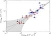 |
Fig. 1 Correlation of N(H2) calculated from dust continuum and from 13CO(1−0) using a 13CO abundance of 10-6. The circles mark the column densities derived from the excitation temperature estimates (where 12CO measurements were available). The vertical error bars show N(H2)gas lower and upper limits calculated using 8.5 and 19.5 K as excitation temperature and the horizontal error bars are from the uncertainty of the τ250 values in the centre of the clumps. The colours indicate the dust colour temperature: blue is below 14 K and red is above 14 K. Where only lower and upper limits of N(H2)gas could be calculated, only error bars are shown with the colour code. The dashed line indicates N(H2)dust = N(H2)gas, the solid line is the linear fit to the plotted values and the shaded area shows the 1σuncertainty range of this fit. |
The Herschel-based dust colour temperatures are more uniform: all the clumps show Tdust values between 12 and 16 K and the histogram peaks at 14 K. The Tdust values do not correlate well with the derived excitation temperatures. The reason for this is that dust and gas in the interstellar matter are only coupled at volume densities above ≈105 cm-3 (Goldsmith 2001), which are typically not traced by our observed molecules. The peak N(H2)dust in the clumps have values from 0.6−40 × 1021 cm-2 but more than half of the clumps have column densities under 1022 cm-2. The densest clumps are G195.74-A, G69.57-A and G70.10-A with peak N(H2)dust ≥ 3 × 1022 cm-2. The Herschel-derived τ250 and Tdust maps of our GCC fields are shown in Fig. B.1, where the 2D Gaussians fitted to the clumps are overplotted and the clump names are shown as well. The parameters of the fitted 2D Gaussians of the clumps are in Table 4. The sizes of the clumps on the plane of the sky have a median value of ten square arcminutes with G71.27-A being the most extended with 34.8 arcmin2 and G189.51-A the smallest with 3.1 arcmin2. The centres of the fitted 2D Gaussian functions are usually very close to the peak position on the Herschel N(H2)dust map. The difference between them is generally under 1.5″, except in the case of G37.49-A and G116.08-A where it is around 15″. The most elongated clumps are G70.10-A, G115.93-A and G141.25-A, while G26.34-A, G39.65-B and G116.08-A are nearly circular. Almost all our clumps are well resolved by the Herschel observations or at least resolved in one direction and marginally resolved in the other direction (G141.25-A, G189.51-A). The peaks of the Herschel-derived N(H2)dust maps coincide with the measured highest integrated intensity values on the 12CO(1−0) five-point maps only in five clumps (G37.49-A, G91.09-A, G95.76-A, G116.08-A, G139.60-A) but a more detailed analysis of the differences of the peaks cannot be made without larger spectral mapping.
The lower and upper limits of the 13CO column densities, N(13CO)l and N(13CO)u are between 0.5−44 ×1015 cm-2, resulting in N(H2)gas line-based column densities of 0.5 − 44 × 1021 cm-2 using a 13CO abundance of 10-6. Figure 1 shows the correlation of N(H2)gas with the Herschel-based peak H2 column densities. The error bars on N(H2)gas represent the interval between the calculated lower and upper limits of the value, while the circles mark the values calculated with the derived excitation temperatures, where possible. The uncertainties of N(H2)dust again come from the error of the τ250 map at the centre position of the clump. The figure shows a similar correlation to the one found by Parikka et al. (2015). The two values have a linear correlation coefficient of r = 0.85 with a 95% confidence interval of 0.72−0.92. We find a linear least-squares fit corresponding to a 13CO abundance of 0.8 ± 0.1 × 10⁻⁶. Considering the uncertainties of the linear fit parameters this is close to the 1−1 correlation. However, as discussed before, optical depth effects of the 13CO emission and the variation of the 13CO relative abundances can shift the fitted line. The real scatter also might be smaller or larger than in the figure. The factors contributing to the uncertainty of gas- and dust-based H2 column densities are summarised in Sect. 4.1. The correlation with Tdust is also shown in the figure with colour code. Clumps with Tdust < 14 K (corresponding to the average dust temperature in our sample) appear only above N(H2)dust = 0.4 × 1022 cm-2, but some warmer clumps with Tdust ≥ 14 K have high column densities, for example G195.74-A with Tdust = 14.3 K has the highest peak N(H2)dust in the sample.
3.3. Clump distances
The distances of more than one hundred GCC fields were provided by Montillaud et al. (2015) using extinction method, kinematic distance calculation (based on the surveys of Dame et al. 2001; and Wu et al. 2012) and association with molecular cloud complexes or star clusters. They included reliability flags with their results that indicate the level of confidence of the adopted distances: a flag equal to two indicates a good level of confidence due to the agreement of the used methods, a value of one indicates a reasonable estimate which needs to be confirmed independently and a value of zero indicates unreliable estimates. They have distance estimates for all but three of our 35 clumps: nine clumps have distances with a reliability flag of two, 15 clumps have distances with a flag of one and eight clumps only have an estimate with a reliability flag of zero. Since the spatial and spectral resolution of our survey is higher than what was used by them, we also performed kinematic distance calculations to assess the confidence of the distance estimation of our clumps, to verify the previous results or provide more reliable numbers. We used the revised method of Reid et al. (2009) and similarly to the work of Montillaud et al. (2015) the kinematic distances were calculated both assuming a source peculiar velocity of 0 km s-1 and −15 km s-1 compared to the rotation of the Galaxy. The error in the 13CO vLSR velocities was assumed to be a conservative value of 1 km s-1.
Kinematic distances of the clumps.
Calculated sizes and masses and adopted distances of the clumps.
We chose the near solution versus the far solution where the two were not equal, since these galactic cold objects are expected to be mostly under 2 kpc distances. This is supported by the fact that most of our clumps (except G91.09-A, G109.18-A and G141.25-A) can be seen in optical extinction maps. The three exceptions have a higher Galactic latitude (around 30°) therefore are likely to be close-by. The far solution can be also rejected in most cases since it generally would imply unrealistic Galactic altitudes, while the vertical scale height of the molecular material in the Galaxy is around 70−80 pc (Bronfman et al. 1988; Clemens et al. 1988). Thus even the near kinematic distance estimates of G71.27-A and G91.09-A will result in very high Galactic altitudes. These distance results were rejected and not used further. The clumps G174.22-A, G174.22-B, G188.24-A and G189.51-A are located close to a Galactic longitude of 180° where the velocity component due to the rotation of the Galaxy is the tangential component which cannot be measured with spectroscopy. Indeed the calculated kinematic distances of these clumps proved to be unrealistic and were not used further. We also note that for nearby clumps distance calculations based on galactic rotational properties are unreliable because peculiar velocities dominate their measured vLSR values.
The calculated kinematic distances of the clumps are listed in Table 5 along with the previously determined distances by Montillaud et al. (2015). The rejected kinematic distance results are marked with an asterisk. In case of clumps with reliability flags of two the previous distance estimates were mostly based on association with cloud complexes. We adopt these estimates for these clumps since either at least one of our kinematic distances is consistent with them or we do not have a reliable result for them from the kinematic method. For most of the clumps with reliability flags of one we also accept the previous estimates because at least one of our kinematic distance results is close to the value determined by extinction methods, making it more reliable. In the case of four clumps (G37.91-A, G37.91-B, G110.62-A and G141.25-A) our kinematic distances were consistent with but somewhat different from previous extinction-based values. Here we have adopted a mean value with a formal error that covers both results. It has already been noted in Sect. 3.1 that we only observed the higher velocity 13CO line component towards the two clumps G37.91-A and G37.91-B. Thus we adopted a higher distance value for them with a smaller error bar that is still consistent with the result of the extinction method but does not cover the kinematic distance calculated from the low velocity component. For G110.62-A our estimate with a vs = −15 km s-1 coincides well with the spectroscopic distances of associated stars derived by Aveni & Hunter (1969), thus we adopted 0.385 ± 0.16 kpc which covers both values. The clump G141.25-A has a distance estimate from spectroscopic analysis of background stars for the Ursa Major complex MBM29−31 that is associated with the clump (Penprase 1993). Our kinematic distance estimate is somewhat higher and a value of 0.215 ± 0.115 kpc was adopted that covers both. The clump G126.24-A had only an extinction-based distance estimate so far. Here our kinematic distance result with vs = −15 km s-1 is consistent with that value and it was accepted. Finally, for the clumps with reliability flags of zero, we were not able to significantly improve the previously determined distances, except in the case of G109.18-A where no kinematic distance calculation existed before. The extinction-based distance cited by Montillaud et al. (2015) is 160 pc (Juvela et al. 2012) but due to the lack of complementary data the value is highly uncertain and received a flag of zero. Our result is much higher than this (around 1 kpc), thus we adopted the mean of the extinction-based and our kinematic result with an appropriately large error bar that covers both values. The clumps G71.27-A, G91.09-A and G171.35-A remain without reliable distance estimates. The final, adopted distances are included in Table 5.
3.4. Clump stability
We use the adopted distances in Table 5 to perform the virial analysis of the clumps. The uncertainties in clump mass are dominated by the error of the distance, since the errors originating from the uncertainties of τ250 and the conversion to N(H2)dust (due to different RV values) are both less than 30%. Through the calculated sizes of the clumps the virial masses are also affected by the distance uncertainty. For this reason we only considered the stability of clumps where the distance values are reasonably reliable: the clumps with a flag of one and two and G109.18-A, where we revised the previously calculated value. The clumps with two velocity components were excluded from this analysis since the dimensions and masses of the two structures corresponding to the velocity components cannot be separated using a column density map. The sizes, masses and virial masses of these clumps are in Table 6, including the lower and upper limits of Mclump clump mass and Mvir virial mass due to the distance uncertainty. The virial mass calculations were done using the two limiting temperatures (8.5 and 19.5 K). The errors of the FWHM sizes were also calculated from the distance uncertainty.
The FWHM sizes of the clumps vary in the range 0.1−5 pc, where the smallest is G141.25-A and the most extended are G70.10-A, G70.10-B and G174.22-A. Considering the error in the distance estimates, clump masses vary from 0.02 M⊙ to more than 1600 M⊙, covering a very wide range of values. From the 22 clumps with virial mass estimates eleven have masses lower than either of the calculated virial masses, making these clumps gravitationally unbound. Except G39.65-A and G62.16-A they all have masses less than around 10 M⊙, are mostly rather small (from 0.18 to 0.5 pc) and are located closer to us (under 0.6 kpc). The rest of the clumps tend to have larger distances and show several hundred solar masses. Their stability cannot be decided with a good reliability because of the large errors caused by the distance uncertainty in both clump masses and virial masses.
4. Discussion
4.1. The temperatures and column densities of the clumps
According to Fig. 1 colder clumps have a peak N(H2)dust> 4 × 1021 cm-2 and N(13CO) > 5 × 1015 cm-2 but while most of the clumps with Tdust above 14 K have lower densities, some of them show high values. The correlation of the peak N(H2)dust and N(H2)gas seems to be good but there are many factors that can affect their relation. As discussed before, the line-based column densities are underestimated due to optical depth effects. The radiative transfer models used to investigate the optical depth and its effect on column density in model clumps with similar densities as in our sample are described in Appendices A.1 and A.2. Using modelling (adopting density-dependent abundances with a maximum value of [13CO]/[H2] = 1.5 × 10⁻⁶) we found that the gas-derived column densities of our model clouds can have values by a factor of two lower than the ones derived from dust emission. Differences between N(H2)dust and N(H2)gas may also originate from the uncertainties of N(H2)dust, the lack of background subtraction and the use of the incorrect dust spectral index.
The agreement of the two values is also affected by the assumed relative abundance of 13CO. Most studies find values close to 2 × 10⁻⁶, like 1.5 × 10⁻⁶ in Taurus and 2.9 × 10⁻⁶ in Ophiuchus (Frerking et al. 1982), 2.3 × 10⁻⁶ in IC 5146 (Lada et al. 1994) or 2.5 × 10⁻⁶ in Perseus (Pineda et al. 2008). Harjunpää et al. (2004) found values between 0.9−3.5 × 10⁻⁶ in their survey of the three globules B 133, B 335 and L 466. We used an abundance of 10-6 in our calculations of N(H2)gas that results in the good agreement seen in Fig. 1. We note that the abundance of 13CO can vary inside a clump as well, especially towards starless clumps due to freeze-out.
We note that although we usually expect Tex to be somewhat lower than Tkin, this may not be always the case. Since CO is not the best in probing the temperatures inside the densest clumps and we get less radiation from the clump centres, the observed Tex could sometimes be higher than Tkin in the centre, even if the true Tex were always locally lower than Tkin. The expected Tex values inside the clumps were checked during the radiative transfer modelling and according to the results we expect the values of Tex and Tkin to be similar (thus the observed Tex limits 8.5 K and 19.5 K were used for the stability calculations as well).
Association with possibly-embedded YSOs could explain the high Tdust or Tex derived for some of the clumps. According to the young star object candidate catalogue by Marton et al. (2016a) 26 of our clumps from the 35 have no associated Class I/II or Class III YSO candidates inside a radius that equals to the major axis of their fitted 2D Gaussian function. The clumps G37.49-A, G37.91-A and B, G69.57-A and B and G139.60-A are associated with 1−1 Class I/II YSO candidates, G39.65-A and G70.10-A have 2 associated Class I/II YSO candidates. The clump G195.74-A is associated with 6 Class I/II YSO candidates. Additionally, 2 Class III YSO candidates were found associated with G70.10-A and 4-4 Class III sources are associated with G37.91-A and G39.65-A (Marton et al. 2016b). As mentioned previously the two clumps with high Tex are clearly associated with YSOs both by Marton et al. (2016a) and Montillaud et al. (2015).
4.2. The nature of the clumps
The ratio of gravitationally bound clumps was five out of 21 clumps by Parikka et al. (2015) in their analysis of a similar GCC sample and most core-sized clumps in our sample also seem sub-critical. However, many of the more distant clumps have large distance uncertainties that makes it difficult to assess their state. There is a group of objects that have physical sizes close to 1 pc or more, masses of more than a few hundred M⊙ and are located at high distances (1−3 kpc). This suggests that they are large-scale clouds or clumps that may contain many smaller clumps or cores which remain unresolved in our observations. Some of our objects have sizes of less than 0.3 pc and are at smaller distances, for example G110.62-A, G116.08-A, G141.25-A or G189.51-A. These objects are closer to the traditional definition of individual cores, seem to be gravitationally unbound and none of them are associated with young stars. We also find gravitationally unbound objects that are larger than cores, like G39.65-A and G126.24-A. The large-scale clouds or clumps are mostly dense with peak N(H2)dust ≳ 1022 cm-2 but they appear with both low and high Tdust and Tex values (e.g. G195.74-A with Tdust = 14.3 K and Tex = 23.4 K is dense and warm, while G174.22-B with Tdust = 12.4 and Tex = 9.5 K is dense but cold). The large ratio of gravitationally unbound, core-sized objects might be explained by the 13CO emission overestimating the velocity dispersion inside the clumps since the line broadening due to optical depth can cause an overestimate of the virial mass by a factor of up to two, according to our models.
We compared the T90% values calculated on the respective GCC fields of our clumps by Montillaud et al. (2015) to the virial state of the clumps. The T90% value gives the temperature below which 90% of the pixels are on the Herschel-derived dust colour temperature maps of the GCC fields and is used as a proxy of the intensity of the local interstellar radiation field. Montillaud et al. (2015) found a correlation between T90% and Galactic radius which is consistent with the radiation field being stronger in the inner Galaxy and examined the relation between this temperature and the cumulative fractions of their sources. A correlation between the boundedness of clumps and the surrounding temperature would mean that clumps are more bound in colder environments. This would support the implication that the heating by the surrounding visible−UV radiation field may prevent the collapse of cores. We find that the average value of T90% is 17.1 K for the gravitationally unbound clumps and 16.4 K for the larger clumps with higher mass and distance where the stability cannot be assessed. This difference is not significant due to the large error in Mclump and Mvir and the usual error of around 1 K in SPIRE-derived dust temperature maps in cold environments.
5. Conclusions
We obtained good S/N, and high spectral and spatial resolution of the 12CO(1−0) and 13CO(1−0) spectra in the direction of 35 clumps on 26 fields selected from the Herschel GCC sample. Based on the molecular line data, Tex and N(13CO) values inside the clumps were calculated and the far-infrared dust continuum maps of Herschel were used to derive Tdust and N(H2)dust distribution.
The clumps in our sample have excitation temperatures generally between 8.5 and 19.5 K, with G195.74-A and G139.60-A showing even higher values, suggesting the presence of embedded YSOs. The derived dust colour temperatures are between 12−16 K. Clumps with temperatures above the average 14 K appear both at low and high column densities but colder clumps have peak N(H2)dust above 4 × 1021 cm-2. The gas- and dust-based column densities of the clumps correlate well but can be affected by many uncertainties from CO optical depth effects to the assumed dust properties. We performed radiative transfer modelling to predict CO emission, optical depths and column densities to verify our results and estimate the uncertainties.
Kinematic distance calculations were performed using 13CO line velocities in an attempt to obtain more reliable values. The previous distance estimates of 5 clumps were refined by our new results. We identified 11 gravitationally unbound clumps in the sample with a few solar masses that are core-sized and are located close-by. Large, massive objects were also found, which are located at larger distances, suggesting that these clouds may contain further cores and clumps. Some of these large objects are associated with YSOs, while no young stars were found around most of the unbound, core-sized sources. The dominant uncertainty in assessing the state of our clumps originates from the large errors in their distance estimates. No correlation was found between the temperature of the surrounding environment and the level of boundedness of the clumps.
In reality, the higher column density would also increase the amount by which continuum analysis underestimates the true column density. Thus, the adopted simple rescaling gives slightly higher and more correct estimates of N(H2).
Acknowledgments
This research was partly supported by the OTKA grants K101393 and NN-111016 and it was supported by the Momentum grant of the MTA CSFK Lendület Disk Research Group. M.J. acknowledges the support of the Academy of Finland Grant No. 285769. T.L. acknowledges the support from the Swedish National Space Board (SNSB). This work was supported by NAOJ ALMA Scientific Research Grant Number 2016-03B. The authors wish to thank the anonymous referee for their valuable comments and suggestions. The Onsala Space Observatory (OSO), the Swedish National Facility for Radio Astronomy, is hosted by Department of Earth and Space Sciences at Chalmers University of Technology, and is operated on behalf of the Swedish Research Council. We thank the staff of OSO for their assistance with the observations. Herschel was an ESA space observatory with science instruments provided by European-led Principal Investigator consortia and with participation from NASA. SPIRE was developed by a consortium of institutes led by Cardiff Univ. (UK) and including Univ. Lethbridge (Canada); NAOC (PR China); CEA, LAM (France); IFSI, Univ. Padua (Italy); IAC (Spain); Stockholm Observatory (Sweden); Imperial College London, RAL, UCL-MSSL, UKATC, Univ. Sussex (UK); Caltech, JPL, NHSC, Univ. Colorado (USA). This development was supported by national funding agencies: CSA (Canada); NAOC (PR China); CEA, CNES, CNRS (France); ASI (Italy); MCINN (Spain); SNSB (Sweden); STFC (UK); and NASA (USA). PACS was developed by a consortium of institutes led by MPE (Germany) and including UVIE (Austria); KUL, CSL, IMEC (Belgium); CEA, OAMP (France); MPIA (Germany); IFSI, OAP/AOT, OAA/CAISMI, LENS, SISSA (Italy); IAC (Spain). This development has been supported by the funding agencies BMVIT (Austria), ESA-PRODEX (Belgium), CEA/CNES (France), DLR (Germany), ASI (Italy), and CICT/MCT (Spain).
References
- Arzoumanian, D., André, P., Didelon, P., et al. 2011, A&A, 529, L6 [Google Scholar]
- Aveni, A. F., & Hunter, Jr., J. H. 1969, AJ, 74, 1021 [NASA ADS] [CrossRef] [Google Scholar]
- Bergin, E. A., & Tafalla, M. 2007, ARA&A, 45, 339 [NASA ADS] [CrossRef] [Google Scholar]
- Bronfman, L., Cohen, R. S., Alvarez, H., May, J., & Thaddeus, P. 1988, ApJ, 324, 248 [NASA ADS] [CrossRef] [Google Scholar]
- Clemens, D. P., Sanders, D. B., & Scoville, N. Z. 1988, ApJ, 327, 139 [NASA ADS] [CrossRef] [Google Scholar]
- Dame, T. M., Hartmann, D., & Thaddeus, P. 2001, ApJ, 547, 792 [NASA ADS] [CrossRef] [Google Scholar]
- Draine, B. T. 2003, ARA&A, 41, 241 [NASA ADS] [CrossRef] [Google Scholar]
- Fehér, O., Tóth, L. V., Ward-Thompson, D., et al. 2016, A&A, 590, A75 [NASA ADS] [CrossRef] [EDP Sciences] [Google Scholar]
- Frerking, M. A., Langer, W. D., & Wilson, R. W. 1982, ApJ, 262, 590 [NASA ADS] [CrossRef] [Google Scholar]
- Glover, S. C. O., Federrath, C., Mac Low, M.-M., & Klessen, R. S. 2010, MNRAS, 404, 2 [NASA ADS] [Google Scholar]
- Goldsmith, P. F. 2001, ApJ, 557, 736 [NASA ADS] [CrossRef] [MathSciNet] [Google Scholar]
- Griffin, M. J., Abergel, A., Abreu, A., et al. 2010, A&A, 518, L3 [Google Scholar]
- Harjunpää, P., Lehtinen, K., & Haikala, L. K. 2004, A&A, 421, 1087 [NASA ADS] [CrossRef] [EDP Sciences] [Google Scholar]
- Juvela, M. 1997, A&A, 322, 943 [NASA ADS] [Google Scholar]
- Juvela, M., & Padoan, P. 2003, A&A, 397, 201 [NASA ADS] [CrossRef] [EDP Sciences] [Google Scholar]
- Juvela, M., Ristorcelli, I., Pagani, L., et al. 2012, A&A, 541, A12 [NASA ADS] [CrossRef] [EDP Sciences] [Google Scholar]
- Juvela, M., Malinen, J., & Lunttila, T. 2013, A&A, 553, A113 [NASA ADS] [CrossRef] [EDP Sciences] [Google Scholar]
- Juvela, M., Demyk, K., Doi, Y., et al. 2015a, A&A, 584, A94 [NASA ADS] [CrossRef] [EDP Sciences] [Google Scholar]
- Juvela, M., Ristorcelli, I., Marshall, D. J., et al. 2015b, A&A, 584, A93 [NASA ADS] [CrossRef] [EDP Sciences] [Google Scholar]
- Lada, C. J., Lada, E. A., Clemens, D. P., & Bally, J. 1994, ApJ, 429, 694 [NASA ADS] [CrossRef] [Google Scholar]
- MacLaren, I., Richardson, K. M., & Wolfendale, A. W. 1988, ApJ, 333, 821 [NASA ADS] [CrossRef] [Google Scholar]
- Malinen, J., Juvela, M., Collins, D. C., Lunttila, T., & Padoan, P. 2011, A&A, 530, A101 [NASA ADS] [CrossRef] [EDP Sciences] [Google Scholar]
- Marton, G., Tóth, L. V., Paladini, R., et al. 2016a, MNRAS, 458, 3479 [NASA ADS] [CrossRef] [Google Scholar]
- Marton, G., Toth, L. V., Paladini, R., et al. 2016b, VizieR Online Data Catalog: J/MNRAS/458/3479 [Google Scholar]
- Meng, F., Wu, Y., & Liu, T. 2013, ApJS, 209, 37 [NASA ADS] [CrossRef] [Google Scholar]
- Montillaud, J., Juvela, M., Rivera-Ingraham, A., et al. 2015, A&A, 584, A92 [NASA ADS] [CrossRef] [EDP Sciences] [Google Scholar]
- Ossenkopf, V., & Henning, T. 1994, A&A, 291, 943 [NASA ADS] [Google Scholar]
- Pagani, L., Lefèvre, C., Juvela, M., Pelkonen, V.-M., & Schuller, F. 2015, A&A, 574, L5 [NASA ADS] [CrossRef] [EDP Sciences] [Google Scholar]
- Palmeirim, P., André, P., Kirk, J., et al. 2013, A&A, 550, A38 [NASA ADS] [CrossRef] [EDP Sciences] [Google Scholar]
- Parikka, A., Juvela, M., Pelkonen, V.-M., Malinen, J., & Harju, J. 2015, A&A, 577, A69 [NASA ADS] [CrossRef] [EDP Sciences] [Google Scholar]
- Penprase, B. E. 1993, ApJS, 88, 433 [NASA ADS] [CrossRef] [Google Scholar]
- Pilbratt, G. L., Riedinger, J. R., Passvogel, T., et al. 2010, A&A, 518, L1 [CrossRef] [EDP Sciences] [Google Scholar]
- Pineda, J. E., Caselli, P., & Goodman, A. A. 2008, ApJ, 679, 481 [NASA ADS] [CrossRef] [Google Scholar]
- Planck Collaboration VII. 2011, A&A, 536, A7 [NASA ADS] [CrossRef] [EDP Sciences] [Google Scholar]
- Planck Collaboration XXIII. 2011, A&A, 536, A23 [NASA ADS] [CrossRef] [EDP Sciences] [Google Scholar]
- Planck Collaboration XXXVIII. 2016, A&A, 594, A28 [NASA ADS] [CrossRef] [EDP Sciences] [Google Scholar]
- Poglitsch, A., Waelkens, C., Geis, N., et al. 2010, A&A, 518, L2 [NASA ADS] [CrossRef] [EDP Sciences] [Google Scholar]
- Reid, M. J., Menten, K. M., Zheng, X. W., et al. 2009, ApJ, 700, 137 [NASA ADS] [CrossRef] [Google Scholar]
- Rivera-Ingraham, A., Ristorcelli, I., Juvela, M., et al. 2016, A&A, 591, A90 [NASA ADS] [CrossRef] [EDP Sciences] [Google Scholar]
- Rohlfs, K., & Wilson, T. L. 1996, Tools of Radio Astronomy (Berlin, Heidelberg, New York: Springer Verlag), 127 [Google Scholar]
- Shetty, R., Kauffmann, J., Schnee, S., Goodman, A. A., & Ercolano, B. 2009a, ApJ, 696, 2234 [NASA ADS] [CrossRef] [Google Scholar]
- Shetty, R., Kauffmann, J., Schnee, S., & Goodman, A. A. I. 2009b, ApJ, 696, 676 [NASA ADS] [CrossRef] [Google Scholar]
- Steinacker, J., Linz, H., Beuther, H., Henning, T., & Bacmann, A. 2016, A&A, 593, L5 [NASA ADS] [CrossRef] [EDP Sciences] [Google Scholar]
- Tauber, J. A., Mandolesi, N., Puget, J.-L., et al. 2010, A&A, 520, A1 [NASA ADS] [CrossRef] [EDP Sciences] [Google Scholar]
- Tóth, L. V., Zahorecz, S., Marton, G., et al. 2016, in From Interstellar Clouds to Star-Forming Galaxies: Universal Processes?, eds. P. Jablonka, P. André, & F. van der Tak, IAU Symp., 315, E75 [Google Scholar]
- Tóth, L. V., Zahorecz, S., Marton, G., et al. 2017, in IAU Symp. 316, eds. C. Charbonnel, & A. Nota, 133 [Google Scholar]
- Wu, Y., Liu, T., Meng, F., et al. 2012, ApJ, 756, 76 [NASA ADS] [CrossRef] [Google Scholar]
- Zahorecz, S., Jimenez-Serra, I., Wang, K., et al. 2016, A&A, 591, A105 [NASA ADS] [CrossRef] [EDP Sciences] [Google Scholar]
- Zhang, T., Wu, Y., Liu, T., & Meng, F. 2016, ApJS, 224, 43 [NASA ADS] [CrossRef] [Google Scholar]
Appendix A: Tests with radiative transfer models
Appendix A.1: Modelling the line emission of Bonnor-Ebert spheres
To further quantify the possible bias of the column density estimates derived from 13CO spectra, we carried out radiative transfer calculations for a series of spherically symmetric models. The density distributions follow the Bonnor-Ebert solutions for a kinetic temperature of 12 K, a stability parameter ξ = 6.7, and with 0.3, 1.0, or 3.0 solar masses. The 12CO abundance is fixed to 5 × 10⁻⁴. The 13CO abundance is varied in a range of 0.3−3.0 times the default value of 10-6. The turbulent linewidth is σv = 1 km s-1 and there is additionally a linear radial velocity gradient that increases from zero at the centre to 1 km s-1 at the cloud boundary (infall).
Line emission depends on the volume density, column density, velocity field, and kinetic temperature of the clouds. A Bonnor-Ebert model may not accurately describe the density profiles of our clumps. However, here it is only necessary that the models cover the relevant parameter space. The selected kinetic temperature and line widths are typical of the values listed in Table 2 and indicated by the Tex values of Table 3. Already for the default abundance of 10-6, the 13CO column densities range from 1015 cm-2 to 1017 cm-2, covering the entire range of column density estimates in Table 3. The mass of the Bonnor-Ebert spheres is a parameter that scales the cloud column density. The model clouds have mean volume densities of 5.5 × 10³, 5 × 10⁴ and 5.5 × 105 cm-3 while the real clumps have peak volume densities between 4.5 × 103 cm-3 and 3.2 × 104 cm-3. Since all used densities are above the CO critical density of 103 cm-3, the model clumps are applicable for calculating excitation.
The radiative transfer calculations give 12CO and 13CO line profiles as a function of the distance from the cloud centre. We calculated the average spectra for emission within 10%, 50%, and 100% of the outer radius of the Bonnor-Ebert spheres. Using the equations of Sect. 2.3.1, the peak antenna temperatures, and the integrated area of the averaged 13CO spectra, we estimated the “observed” 13CO column densities. For comparison, we extracted directly from the cloud models the area-averaged values of the peak 13CO optical depth and the true 13CO column density. These were averaged over the same regions as the synthetic observations, to allow direct comparison.
Figure A.1 shows the ratio of the observed and the true column densities as a function of the true 13CO optical depth. The ratio is mainly a function of the optical depth. The averaging of the emission over the whole cloud results in some 20% lower values (relative to the true values) than when the spectra represent the inner 10% of the model clouds. The main parameter affecting the ratio of observed and true column densities is the line optical depth. When the average optical depth of the 13CO line is close to one, the observations underestimate the true column density by 20−40%. In these models, the error is likely to remain below 50% up to optical depths of about τ = 3.
Appendix A.2: Modelling the continuum and line emissions of two fields
To quantify the potential systematic errors in the column density estimates, we carried out radiative transfer modelling of the continuum (Juvela & Padoan 2003; Juvela, in prep.) and the line emission (Juvela 1997) for the fields G26.34+8.65 and G195.74-2.29, where the column densities are representative of the column density range of our clump sample. The models correspond to a projected area of 30 × 30′, which is much larger than the size of the clumps, to avoid any border effect (e.g. strong temperature gradients near the model boundaries).
In the first stage, we create 3D cloud models that reproduce the Herschel dust continuum observations at 250 μm, 350 μm, and 500 μm. The models consist of 2003 cells with a cell size equal to 9″ on the sky. The dust properties are taken from Ossenkopf & Henning (1994) and correspond to thin ice mantles (after 105 yr at density 106 cm-3). The model is appropriate mainly for the densest regions. However, in this context one of the most relevant parameters is the assumed ratio of hydrogen column density to sub-millimetre opacity, which affects the density field used in the following line modelling. In our basic models this is τ250/N(H2) = 1.52 × 10⁻²⁴ cm2. However, the assumptions in Sect. 2.4 correspond to a value that is almost twice as large and would thus result in model clouds with higher N(H2)dust values and potentially larger problems for the column density estimation. Thus, in the line modelling, we will also test a case where the density values obtained from the continuum modelling are scaled by a factor of 2. The density distribution in the plane of the sky is constrained by the continuum observations. Along the line of sight, the density is assumed to follow a profile ![Mathematical equation: \appendix \setcounter{section}{1} \begin{equation} \rho(x) \propto \left[1+(x/R)^2 \right]^{-p/2}, \end{equation}](/articles/aa/full_html/2017/10/aa29866-16/aa29866-16-eq160.png) (A.1)where x is the line-of-sight distance from the model mid-plane, R is set to a distance that corresponds to one arcmin on the sky, and p = 2. The uncertainty of the density distribution along this axis is a significant source of uncertainty. However, for the adopted parameters the clumps have roughly similar extent along the line of sight and in the plane of the sky.
(A.1)where x is the line-of-sight distance from the model mid-plane, R is set to a distance that corresponds to one arcmin on the sky, and p = 2. The uncertainty of the density distribution along this axis is a significant source of uncertainty. However, for the adopted parameters the clumps have roughly similar extent along the line of sight and in the plane of the sky.
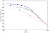 |
Fig. A.1 Ratio of the observed and the true 13CO column densities for synthetic observations of Bonnor-Ebert spheres. There are three sets of curves that corresponds to cloud masses of 0.3, 1.0, and 3.0 solar masses (from right to left, colours red, green, and blue, respectively). The solid, dashed, and dotted lines refer to averaging of the data (observed intensity and true values) within 10%, 50%, and 100% of the cloud outer radius. The length of each line corresponds to a variation of the 13CO abundance between 0.3 and 3 times the default value of 10-6. |
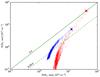 |
Fig. A.2 Comparison of column densities derived from radiative transfer models of continuum and line emission. The dots correspond to all the pixels within the central 15′ × 15′ areas of the G26.34+8.65 (blue dots) and G195.74-2.29 (red dots) models. The coloured circles correspond to the positions of the clumps listed in Table 1. The crosses denote the column density estimates obtained assuming Tex = 14 K. |
The continuum observations are fitted in an iterative manner. The strength of the external radiation field is scaled based on the observed and modelled ratios between the 250 μm and 500 μm bands. The ratios are estimated as averages over the central area of 15 × 15′. The 350 μm data are used, pixel by pixel, to adjust the model column densities. The procedure leads to a model that reproduces the 350 μm surface brightness (final relative errors below ~1%) and gives the correct average shape of the dust emission spectrum. In practice, the relative model errors at 250 μm and 500 μm are also typically no more than ~3%. The procedure results in a 3D model of the density field and also provides synthetic surface brightness maps at the three Herschel wavelengths. The surface brightness maps were analysed in a way similar to the actual observations, resulting in 200 × 200 pixel maps of the dust optical depth. Because the 250−500 μm spectral index of the employed dust model is β = 1.92 instead of β = 2.0, the dust-derived column densities are systematically overestimated but only by ~ 10%.
In the second stage, we used the derived density cube for the radiative transfer modelling of the 12CO and 13CO lines. We assumed a maximum fractional abundance of 1.5 × 10⁻⁶ for 13CO (Frerking et al. 1982; Harjunpää et al. 2004). The abundances are further scaled by a factor  (A.2)which depends on the local H2 density, n (in units cm-3). With this scaling, the maximum abundance is reached only at densities above n = 103 cm-3. The scaling still results in a faster rising of abundance (as a function of density) than most of the models discussed in Glover et al. (2010). The gas kinetic temperature is set to a constant value of 15 K. The model includes two components of the velocity field, one below the model resolution (microturbulence within individual cells) and one as random velocities between the cells. We assumed that the two components are equal and together correspond to the observed 13CO line widths, under the assumption of optically thin line emission.
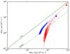 |
Fig. A.3 Comparison of column densities derived from radiative transfer models where the densities have been increased by a factor of two. |
The line radiative transfer modelling results in maps of 200 × 200 12CO and 13CO spectra, each with a velocity resolution of 0.07 km s-1. We processed these in a way similar as the actual observations. The spectra are fitted with Gaussian functions and the analysis results in maps of the estimated 13CO column density, also at 9″ resolution. However, when Tex is derived from the 12CO, we use the actual peak temperature instead of the peak of the fitted Gaussian. Unlike in the real observations, the modelled 12CO spectra are strongly self-absorbed and in the densest regions therefore clearly double-peaked.
Figure A.2 shows the result of the modelling exercise with the default densities. On the x-axis are the dust-derived column densities where the scaling between dust optical depth and column density is done using a conversion factor that is correct for the used dust model. On the y-axis are the estimates derived from the synthetic line spectra, using the adopted maximum 13CO abundance used in the modelling. At low column densities the gas-derived column density is more than four times below the dust-derived values, because the true abundance is lower than assumed in the conversion to N(H2). For the lines of sight towards the clumps, where the abundance should already have reached its maximum value, the difference to dust column density is smaller. However, the results are also different for the positions of the two clumps, which are marked in the figure as coloured circles. The estimated 13CO optical depths are mostly below one but do rise to 1−1.5 in the two clumps.
Figure A.3 shows the results when the densities are set higher by a factor of two. The dust-derived column densities were simply multiplied by two3 but the line calculations were repeated, starting with the simulations of the radiative transfer.
The modelling suggests that, as long as the dust opacity and the 13CO abundance used in the analysis are correct, there should exist a fairly good correlation between the two column density estimates. This is true only for the densest regions while in the more diffuse regions the line-derived estimates decrease rapidly because of the decreasing fractional abundances. In the higher density models (more consistent with the assumptions of Sect. 2.4) the line analysis would be expected to lead to column densities that are by a factor of two lower than the values derived from dust emission.
Appendix B: Herschel τ250 and Tdust maps
Figures B.1 show the optical depths of the clumps on 250 μm and their dust colour temperature maps based on Herschel measurements. The 2D Gaussians fitted to the clumps and the respective clumps are indicated.
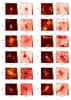 |
Fig. B.1 Herschel-based τ250 and Tdust maps of the clumps. Black ellipses mark the 2D Gaussians fitted to the clumps and they are marked with the letter ID of the respective clumps. A white ellipse in the lower left corner shows the beam size of the Herschel map (37″). |
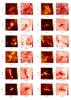 |
Fig. B.1 continued. |
Appendix C: Spectra
Figure C.1 show the 12CO(1−0) and 13CO(1−0) spectra observed at the central position of each clump. The Gaussian profile fit(s) to the lines are shown. Where only 13CO(1−0) measurements were made, only one box appears.
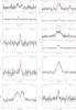 |
Fig. C.1 12CO(1−0) and 13CO(1−0) spectra at the central position of each observed clump. Red line shows the Gaussian profile fit(s) to the lines. |
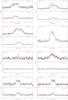 |
Fig. C.1 continued. |
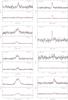 |
Fig. C.1 continued. |
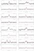 |
Fig. C.1 continued. |
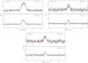 |
Fig. C.1 continued. |
All Tables
All Figures
|
Fig. 1 Correlation of N(H2) calculated from dust continuum and from 13CO(1−0) using a 13CO abundance of 10-6. The circles mark the column densities derived from the excitation temperature estimates (where 12CO measurements were available). The vertical error bars show N(H2)gas lower and upper limits calculated using 8.5 and 19.5 K as excitation temperature and the horizontal error bars are from the uncertainty of the τ250 values in the centre of the clumps. The colours indicate the dust colour temperature: blue is below 14 K and red is above 14 K. Where only lower and upper limits of N(H2)gas could be calculated, only error bars are shown with the colour code. The dashed line indicates N(H2)dust = N(H2)gas, the solid line is the linear fit to the plotted values and the shaded area shows the 1σuncertainty range of this fit. |
| In the text | |
|
Fig. A.1 Ratio of the observed and the true 13CO column densities for synthetic observations of Bonnor-Ebert spheres. There are three sets of curves that corresponds to cloud masses of 0.3, 1.0, and 3.0 solar masses (from right to left, colours red, green, and blue, respectively). The solid, dashed, and dotted lines refer to averaging of the data (observed intensity and true values) within 10%, 50%, and 100% of the cloud outer radius. The length of each line corresponds to a variation of the 13CO abundance between 0.3 and 3 times the default value of 10-6. |
| In the text | |
|
Fig. A.2 Comparison of column densities derived from radiative transfer models of continuum and line emission. The dots correspond to all the pixels within the central 15′ × 15′ areas of the G26.34+8.65 (blue dots) and G195.74-2.29 (red dots) models. The coloured circles correspond to the positions of the clumps listed in Table 1. The crosses denote the column density estimates obtained assuming Tex = 14 K. |
| In the text | |
|
Fig. A.3 Comparison of column densities derived from radiative transfer models where the densities have been increased by a factor of two. |
| In the text | |
|
Fig. B.1 Herschel-based τ250 and Tdust maps of the clumps. Black ellipses mark the 2D Gaussians fitted to the clumps and they are marked with the letter ID of the respective clumps. A white ellipse in the lower left corner shows the beam size of the Herschel map (37″). |
| In the text | |
|
Fig. B.1 continued. |
| In the text | |
|
Fig. C.1 12CO(1−0) and 13CO(1−0) spectra at the central position of each observed clump. Red line shows the Gaussian profile fit(s) to the lines. |
| In the text | |
|
Fig. C.1 continued. |
| In the text | |
|
Fig. C.1 continued. |
| In the text | |
|
Fig. C.1 continued. |
| In the text | |
|
Fig. C.1 continued. |
| In the text | |
Current usage metrics show cumulative count of Article Views (full-text article views including HTML views, PDF and ePub downloads, according to the available data) and Abstracts Views on Vision4Press platform.
Data correspond to usage on the plateform after 2015. The current usage metrics is available 48-96 hours after online publication and is updated daily on week days.
Initial download of the metrics may take a while.