| Issue |
A&A
Volume 601, May 2017
|
|
|---|---|---|
| Article Number | A72 | |
| Number of page(s) | 18 | |
| Section | Planets and planetary systems | |
| DOI | https://doi.org/10.1051/0004-6361/201526215 | |
| Published online | 04 May 2017 | |
Faint warm debris disks around nearby bright stars explored by AKARI and IRSF⋆
1 Department of Physics, Nagoya University, Furo-cho, Chikusa-ku, Nagoya , 464-8602 Aichi, Japan
e-mail: ishihara@u.phys.nagoya-u.ac.jp
2 Department of Physics and Astronomy, Kagoshima University, 1-21-35, Korimoto, 890-0065 Kagoshima, Japan
3 Subaru Telescope, National Astronomical Observatory of Japan, 650 North A’ohoku Place, Hilo, HI 96720 , USA
4 Department of Astronomy, Graduate School of Science, University of Tokyo, 7-3-1 Hongo, Bunkyo-ku, 113-0033 Tokyo, Japan
Received: 30 March 2015
Accepted: 12 June 2016
Context. Debris disks are important observational clues for understanding planetary-system formation process. In particular, faint warm debris disks may be related to late planet formation near 1 au. A systematic search of faint warm debris disks is necessary to reveal terrestrial planet formation.
Aims. Faint warm debris disks show excess emission that peaks at mid-IR wavelengths. Thus we explore debris disks using the AKARI mid-IR all-sky point source catalog (PSC), a product of the second generation unbiased IR all-sky survey.
Methods. We investigate IR excess emission for 678 isolated main-sequence stars for which there are 18 μm detections in the AKARI mid-IR all-sky catalog by comparing their fluxes with the predicted fluxes of the photospheres based on optical to near-IR fluxes and model spectra. The near-IR fluxes are first taken from the 2MASS PSC. However, 286 stars with Ks < 4.5 in our sample have large flux errors in the 2MASS photometry due to saturation. Thus we have measured accurate J, H, and Ks band fluxes, applying neutral density (ND) filters for Simultaneous InfraRed Imager for Unbiased Survey (SIRIUS) on IRSF, the φ1.4 m near-IR telescope in South Africa, and improved the flux accuracy from 14% to 1.8% on average.
Results. We identified 53 debris-disk candidates including eight new detections from our sample of 678 main-sequence stars. The detection rate of debris disks for this work is ~8%, which is comparable with those in previous works by Spitzer and Herschel.
Conclusions. The importance of this study is the detection of faint warm debris disks around nearby field stars. At least nine objects have a large amount of dust for their ages, which cannot be explained by the conventional steady-state collisional cascade model.
Key words: circumstellar matter / zodiacal dust / infrared: stars
The full version of Table 2 is only available at the CDS via anonymous ftp to cdsarc.u-strasbg.fr (130.79.128.5) or via http://cdsarc.u-strasbg.fr/viz-bin/qcat?J/A+A/601/A72
© ESO, 2017
1. Introduction
Debris disks are optically thin circumstellar dust disks around main-sequence stars whose proto-planetary disks have been dissipated. One of the possible scenarios is that they provide important observational clues for understanding planetary-system formation process because the dust grains in these systems may be supplied by collisions between planetesimals or growing proto-planets (e.g., Wyatt 2008).
Observationally, debris disks are detected as infrared (IR) excess emission above the expected photospheric emission of dwarf stars. Debris disks were first reported in 1980s based on the Infrared Astronomical Satellite (IRAS) infrared all-sky survey observations. Including Vega (Aumann et al. 1984), an appreciable number of IR excess stars were reported (Oudmaijer et al. 1992; Mannings & Barlow 1998). Most of them have excess emission at a wavelength of 60 μm. Subsequently, in the 1990s, the detection rate and the timescale of dissipation of debris disks were investigated (Habing et al. 2001; Spangler et al. 2001) using the Infrared Space Observatory (ISO). In the last decade, the Spitzer and Herschel space telescopes detected hundreds of debris disks. The detection rate of debris disks is found to be 10−30% (e.g., Trilling et al. 2008; Eiroa et al. 2013).
The time scale for the dissipation of debris disks, which reflects the time scale of planetary-system formation, is statistically investigated for A-type and FGK-type stars, separately (e.g., Rieke et al. 2005; Su et al. 2006; Siegler et al. 2007). Even in the era of observatory-type IR telescopes, the importance of unbiased surveys is realized through the studies based on the IRAS database (e.g., Rhee et al. 2007). In 2010s, the Wide-field Infrared Survey Explorer (WISE; Wright et al. 2010) has explored large amount of debris disks with a highly sensitive all-sky survey (e.g., Patel et al. 2014).
Though the number of stars in debris-disk samples has been increased, mysteries still remain over in essential points. For example, no simple statistical relation is found between debris disks and planet-hosting stars (Greaves et al. 2006; Moro-Martin et al. 2007; Kospal et al. 2009; Bryden et al. 2009; Dodson-Robinson et al. 2011; Moro-Martin et al. 2015), though debris disks must be observational clues to ongoing planetary-system formation. This might be because the current exoplanet samples and debris-disk samples are weighted toward hot-Jupiters in close orbits and younger, heavier disks, respectively. In addition to the Asteroid and Kuiper belts, our solar system of 4.6 Gyr old also has an optically thin dust disk named the Zodiacal cloud (e.g., Kelsall et al. 1989; Rowan-Robinson & May 2013; Planck Collaboration XIV 2014). The relation between the Zodiacal cloud and debris disks is also an important subject for discussion. One of the promising approaches for these subjects is a systematic exploration of faint debris disks in inner orbits at late stages of planetary system formation.
AKARI is the first Japanese IR astronomical satellite (Murakami et al. 2007) with a 70 cm-diameter 6 K telescope (Kaneda et al. 2007). The AKARI mid-IR all-sky survey was performed with two photometric bands centered at wavelengths of 9 and 18 μm using one of the on-board instruments, the Infrared Camera (IRC; Onaka et al. 2007) simultaneously with the far-IR survey conducted at the 65, 90, 140, and 160 μm bands (Kawada et al. 2007). The AKARI all-sky survey is the second generation unbiased all-sky observation in the IR following the IRAS survey. The publicly available mid-IR all-sky point source catalog (PSC; Ishihara et al. 2010) contains a large amount of newly detected IR sources (e.g., Ishihara et al. 2011), as a result of improvements in sensitivity and spatial resolution over the IR all-sky survey by IRAS (Neugebauer et al. 1969). Among the AKARI bands, the 18 μm band is sensitive to the IR radiation from warm dust grains with temperatures of 100−300 K, which are comparable to the equilibrium temperatures for dust grains at around 1 au from a solar-type star. The detection limit for the AKARI 18 μm band is 90 mJy. In total, 194 551 objects in the PSC have 18 μm detections. In the previous study using the AKARI PSC, we reported 24 debris-disk candidates with large excess emission in the AKARI 18 μm band based on conservative criteria (Fujiwara et al. 2013). Various kinds of minerals were detected through by follow-up observations of newly detected debris-disk candidates. Their conditions for formation give us information on events in the planetary-system formation stages (Fujiwara et al. 2009, 2010). Thus, further systematic exploration of debris disks based on this database is warranted.
In this paper, we explore debris-disk candidates using the AKARI/IRC mid-IR PSC ver. 1 to enable statistical discussions on the evolution of debris disks, their relation to planetary system formations, and the relation between debris disks and the zodiacal light.
2. Observations and data analyses
Debris disks are detected as IR excess emission around main-sequence stars. First, we list known main-sequence stars with 18 μm detections. Then we predict their photospheric fluxes at 18 μm based on the optical to near-IR fluxes and model spectra. Finally, we compare the predicted fluxes with the observed fluxes and investigate excess emission.
2.1. Sample selection
We first obtain 1735 main-sequence candidates that have AKARI 18 μm fluxes. 977 objects are selected from the Tycho-2 spectral type catalog (Wright et al. 2003) while 758 objects are from the Hipparcos catalog (Perryman et al. 1997). We select B8V–M9V stars based on the Tycho-2 spectral type catalog (Wright et al. 2003), which contains the largest number of stars with information on the luminosity class. The Tycho-2 spectral type catalog is made by combining other original catalogs. The luminosity classes for most of the stars are quoted from Michigan catalog for HD stars, Vol. 1−5 (Houk & Cowley 1975; Houk 1978, 1982; Houk & Smith-Moore 1988; Houk & Swift 1999). These catalogs cover the southern hemisphere (Dec < + 5°) with the limiting magnitude of V ~ 15 mag, which is deep enough to cover all the main-sequence stars detected by the AKARI mid-IR survey. To cover stars in the northern hemisphere, we also search for main-sequence stars from the Hertzsprung-Russell (HR) diagram made by using the Hipparcos catalog (Perryman et al. 1997). Stars located in the main-sequence locus (MV < 6.0 × (B−V)−2.0) are added to our sample. A total 64 209 main-sequence candidates are listed and cross-identified with the AKARI mid-IR PSC sources using a search radius of 3′′, because the astrometric accuracy for the Hipparcos catalog, Tycho-2 spectral catalog, and the AKARI mid-IR PSC are ~0.7 milli-arcsec, ~0.5′′, and 2′′, respectively (Perryman et al. 1997; Wright et al. 2003; Ishihara et al. 2010).
Then we carefully screen the 1735 targets using the SIMBAD database to make a clean sample of isolated main-sequence stars. Table 1 summarizes the classification of our main-sequence candidates by the SIMBAD database. Based on the SIMBAD classification, suspected proto-planetary disks and mass-losing stars are removed from our sample, because their IR excess emission tends to be misinterpreted as signs of debris disks. Suspected binary stars, multiple stars, and stars in clusters are also rejected from our sample because it requires further detailed analyses to evaluate contamination in IR fluxes from their companion or neighboring objects. Finally, 750 objects classified as star, high-proper motion star, and extra-solar planet candidate are selected for our analyses.
Classification of our dwarf sample by the SIMBAD database.
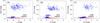 |
Fig. 1 Measurement errors from 2MASS (squares) and IRSF (crosses) as a function of the magnitude in the a) J band, b) H band, and c) Ks band. |
2.2. Photometric data for central stars
We create optical to near-IR spectral energy distributions (SEDs) of the central stars using archival data. The SED for each central star contains five to seven photometric fluxes. The BT and VT band fluxes are taken from the Tycho-2 spectral type catalog (Wright et al. 2003). The J, H, and Ks band fluxes are taken from 2MASS PSC ver. 6 (Cutri et al. 2003). We also add the R-, and I-band fluxes from the Catalog of stellar photometry in Johnson’s 11-color system (Ducati 2002), if available.
2.3. J, H, Ks photometry by IRSF/SIRIUS
Detection of IR excess emission needs accurate estimation of photospheric emission as well as accurate measurement in the mid-IR. The fluxes in the J, H, and Ks bands play important roles to determine photospheric emission accurately. Stars in our sample have fluxes of magnitude one to six in the Ks band. Most of them are too bright to measure their fluxes accurately due to the low saturation limit of 2MASS. Since bright stars are evaluated by point spread function (PSF) fitting of saturated images (Skrutskie et al. 2006), the measurement errors by 2MASS are as large as 11−17% in the J, H, and Ks bands for stars with J< 5.5, H< 5.2, or Ks < 4.5 (see Fig. 1). Thus we have improved the accuracy of photometry of 325 bright main-sequence stars in the J, H, and Ks bands by using the Simultaneous InfraRed Imager for Unbiased Survey (SIRIUS) on InfraRed Survey Facility (IRSF), where SIRIUS is a wide field (7′ × 7′) near-IR camera which enables simultaneous observations in the J, H, and Ks bands (Nagayama et al. 2003) and IRSF is the φ 1.4 m near-IR telescope located at Sutherland in South Africa and managed by Nagoya University (Sato et al. 2001). Table 2 summarizes photometric results for our sample observed by IRSF. With these observations we have successfully improved the J, H, and Ks flux errors from 17% to 1.9%, 14% to 1.4%, and 11% to 2.0%, respectively (see Fig. 1). The details of the observations are given in Appendix A.
2.4. Removing suspected giant stars based on near-IR colors
By using the improved J, H, and Ks fluxes, 39 suspected late-type giant stars are removed from our sample because they show giant-like colors in the J–H versus H–Ks color−color diagrams (see Fig. A.3b). Giants with spectral type later than K1 show different JHK colors from dwarfs while earlier-type giants show similar JHK colors as dwarfs in the JHK color−color plane. We also remove similarly 33 suspected giant stars from the 2MASS based sample (see Fig. A.3a). Finally, a main-sequence sample with 678 stars is obtained.
J, H, Ks magnitudes of bright main-sequence stars measured by IRSF.
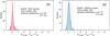 |
Fig. 2 a) Distributions of the excess ratio ((F18,obs−F18, ∗) /F18, ∗) for our sample with IRSF measurements. The center of the peak, μ, and the standard deviation, σ, of the Gaussian distribution are indicated in the graphs. b) Same as a), but for the sample with 2MASS measurements. |
2.5. Estimation of 18 μm photospheric flux
The photospheric flux densities of our sample are calculated from a Kurucz model (Kurucz 1992) fitted to the optical to near-IR photometry of the stars taking extinction into account. In the fitting, the scale factor S (i.e., the distance indicator related to the distance between the star and the Earth), and the visual extinction AV are set as a free parameter, while the effective temperature Teff, metallicity M, and log (g) are selected from discrete sets of template1 values (g is surface gravity in cgs units). The error caused by using quantized parameters for the fitting is discussed in Appendix C. The quantized parameters cause uncertainties for individual F∗, but they are much smaller than the systematic uncertainties for the excess identification. The range of AV is limited between 0 and 0.5 under the assumption that AV is small in most directions within D< 100 pc (Lallement et al. 2003). Teff is allowed to vary within ±1000 K around the initial value that is quoted from the SIMBAD database or estimated from the spectral type. log (g) is selected among 4.0, 4.5, and 5.0, because log (g) for dwarfs varies from 4.2 to 4.7 (Cox et al. 2010). We assume solar metallicity for all the objects because they are located within 600 pc and no significant change in metallicity is expected. For the foreground extinction, we adopt the extinction curve of 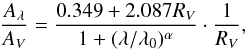 (1)where λ0 = 0.507μm (i.e., V band), Aλ and AV are the extinction at λ and in the V band, respectively, and RV ≡ AV/E(B−V). This is the generalized extinction curve given by Fitzpatrick & Massa (2009) based on the model by Pei (1992). The dust properties in the lines of sight determine RV and α. We use α = 2.05 and RV = 3.11 following Fujiwara et al. (2013), assuming that the extinction curve is uniform within our survey volume. Though this extinction curve does not take into consideration the silicate feature at 10 μm, it does not affect the SED fitting of the photosphere because we only use 0.3−2.4 μm (from U to Ks bands) for the fitting. We might overestimate the photospheric emission at 18 μm because the model (Fitzpatrick & Massa 2009) does not take account of the silicate 18 μm feature. It works as a conservative estimate for the IR excess identification. The reliability of the fitting results is discussed in Appendix B.
2.6. AKARI 18 μm photometry
At the next step, we compare the predicted photospheric fluxes (F18, ∗) with the fluxes (F18,obs) observed at λ = 18μm using the AKARI mid-IR PSC. The monochromatic fluxes in the PSC are derived for objects with spectra of Fλ ∝ λ-1. We apply color corrections to the catalog values assuming that the spectra of the photospheres of main-sequence stars are give by Fλ ∝ λ-4.
2.7. Excess identification
We investigate 18 μm excess emission for each star as follows: the excess ratio at 18 μm, (F18,obs−F18, ∗) /F18, ∗, is calculated for each star. Then we make histograms of the excess ratios for the AKARI-IRSF sample and the AKARI-2MASS sample, separately, as shown in Fig. 2. We fit these histograms with a Gaussian, assuming that these distributions are mainly caused by photon noise. We obtain the center of the peak μ = 0.157 ± 0.005 and standard deviation σ = 0.126 ± 0.005 of the Gaussian function for the AKARI-IRSF sample, while μ = 0.177 ± 0.003 and σ = 0.182 ± 0.003 for the AKARI-2MASS sample. We regard that μ and σ are the systematic offset and the total uncertainties of the sample, respectively. We then select objects as debris-disk candidates which show excess ratios larger than μ + 3σ for both samples.
Then, we check the known extragalactic sources around the excess objects using the NED database in order to avoid incorrect excess identifications by chance alignment of background sources. Even the nearest NED source (1RXSJ194816.6+592519 for HD 187748) aparts as far as 10.02′′. For all the other objects, there are no counter parts within 12′′ which corresponds to the twice of the FWHM of the AKARI 18 μm PSF (5.7′′; Onaka et al. 2007)). Finally, for all the debris-disk candidates, we check the 2MASS Ks, AKARI 9 μm, and AKARI 18 μm images to investigate the effects of image artifacts, and the contamination of background or foreground sources. Details are in Appendix D.
The differences from our previous work (Fujiwara et al. 2013) in the process for identifying debris disks are as follows:
-
Flux accuracy of the central stars: we have improved fluxaccuracy of the photosphere for nearby bright stars (325 objectswith Ks < 4.5) by follow-up observations using IRSF instead of using publicly-available 2MASS fluxes.
-
Sample selection: in this work, we exclude double stars, multiple stars, spectroscopic binaries, and stars in a cluster as well as suspected YSOs and mass-losing stars before investigating the excess emission to discuss the excess probability more accurately. 13 objects out of the 24 debris-disk candidates reported in Fujiwara et al. (2013) are again listed in the current list while 11 objects are not included in our list because they are multiple stars.
3. Results
3.1. Debris-disk candidates with AKARI 18 μm excess emission
As a result, 53 objects out of 678 main-sequence stars in our sample are identified as debris-disk candidates that have excess emission at the AKARI 18 μm band. Tables 3 and 4 summarize the parameters of our debris-disk candidates, for the 2MASS based sample and IRSF based sample, respectively. Figure F.1 shows the SEDs of the individual objects.
It should be noted that some objects show flux ratios much larger than expected for main sequence stars. HD 93942, HD 145263, HD 165014, HD 166191, and HD 167905 are classified as main-sequence stars in literature (Wright et al. 2003), and HD 9186 and HD 215592 has no luminosity class information in literature and were identified as main-sequence stars from the location on the HR diagram. All of them are reported as debris disks candidates in previous works (Oudmaijer et al. 1992; Clarke et al. 2005; McDonald et al. 2012; Fujiwara et al. 2013). It should be noted that HD 166191 was studied by both Schneider et al. (2013) and Kennedy et al. (2014) and the conclusions were different. Additional observations are certainly needed to clarify the nature of these objects. HD 93942 shows a transitional-disk like SED composed of photosphere and thick circumstellar emission. It should also be noted that B- and A-type stars, HD 161840, HD 32509, HD 9186, HD 118978, and HD 28375, show ambient circumstellar emission on the AKARI 18 μm images. These objects are marked in Tables 3 and 4.
List of debris-disk candidates with the AKARI 18 μm excess emission (the 2MASS based sample).
List of debris-disk candidates with AKARI 18 μm excess emission (the IRSF based sample).
3.2. Reliability of mid-IR excess identification
Among the 53 debris-disk candidates, 17 objects have been reported as debris disks in the previous studies (Rieke et al. 2005; Bryden et al. 2006; Su et al. 2006; Trilling et al. 2008; Fujiwara et al. 2013), and the other 28 objects have been reported as mid-IR excess candidates (Oudmaijer et al. 1992; Clarke et al. 2005; McDonald et al. 2012). For evaluating the reliability of our excess estimate, we compare the excess ratio in our results with those in the previous works in Fig. 3 though the observed wavelengths are not exctly the same. Figure 3 indicates that our estimate of the 18 μm excess is consistent with the results in the previous works. Excess ratios at the WISE 22 μm and IRAS 25 μm bands tend to be larger than those at the AKARI 18 μm band, which is reasonable if these systems have circum-stellar dust with temperatures lower than ~300 K. It also confirms that at least our excess ratios are not overestimated.
The available measurements with WISE and IRAS are also overlaid on the individual SEDs in Fig. F.1. Some stars, HD 225132, HD 1237, HD 9186, HD 10939, show discrepancy between the AKARI and WISE-based measurements. It could be attributed to a temporal variation of the dust emission between 2006 and 2010. Another possibility is an effect of the silicate emission features that have broad peaks at 9 and 18 μm. We will address the nature of these objects in future work.
 |
Fig. 3 Flux ratio (Fdisk/F∗) in the previous works plotted against the flux ratio (for the AKARI 18 μm) in this work for the same stars. The filled circles, open circles, filled squares, filled diamonds, pluses, crosses, open triangles, and open squares indicate the flux ratios for the AKARI 18 μm data by Fujiwara et al. (2013), those by McDonald et al. (2012), the WISE 22 μm data by McDonald et al. (2012), the IRAS 25 μm data by McDonald et al. (2012), the Spitzer/MIPS 24 μm data by Su et al. (2006), those by Rieke et al. (2005), those by Trilling et al. (2008), and those by Bryden et al. (2006), respectively. For reference, the red, orange, yellow, green, and blue lines indicate locations in this plot when the disk emission is the blackbody with T = 800, 400, 200, 100, and 50 K, respectively. The dashed lines correspond to the Spitzer 24 μm flux, and dash-dot-dashed lines correspond to the WISE 22 μm flux. |
3.3. Characteristics of our sample
Figure 4 shows the distance versus spectral type for our sample. The detection limit and survey depth, is a function of the spectral type, which is determined by the sensitivity of the AKARI mid-IR PSC. From our sample and the detections shown in Fig. 4, the survey depth for 3σ detections of the photosphere reaches a distance of 74 pc for A0-type stars and 10 pc for M0-type stars. The detection rate of debris disks for the AKARI–2MASS sample is 7.9% (31 objects out of 392). That for the AKARI–IRSF sample, which covers nearby bright stars, is 7.7% (22 objects out of 286), which is comparable to that for the AKARI–2MASS sample. If we use 2MASS fluxes for the AKARI–IRSF sample, the detection rate of debris disks was 2.8% (8 objects out of 286). The IRSF measurements significantly improve the detection rate.
Tables 3 and 4 list the debris-disk candidates detected by AKARI, which include previous disk detections. As shown in the list, eight objects are new detections and 28 objects are confirmation of the previous reports for IR excess detection (Oudmaijer et al. 1992; Clarke et al. 2005; McDonald et al. 2012). In our sample with 2MASS photometry, newly detected objects around B-type stars (HD 146055) were not often explored in previous studies. Our accurate determination of photospheric emission by the IRSF observations results in new debris-disk detection around nearby bright F, and G-type stars (HD 69897, HD 101563, HD 112060, HD 134060, and HD 193307). Therefore our sample contains mostly faint warm disks around bright nearby field stars.
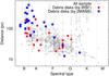 |
Fig. 4 Distance plotted as a function of the spectral type for our sample. The open circles indicate all the 678 sample. The filled circles and filled boxes indicate the debris-disk candidates with the IRSF and 2MASS measurements, respectively. The dotted curve indicates the detection limit for objects without IR excess according to our definition. |
4. Discussion
4.1. Debris-disk detection rate
Table 5 summarizes the total number of our main-sequence stars, the number of debris-disk candidates, and the debris-disk detection rate for each spectral type. The debris-disk frequency varies smoothly from 13% of the A-type to 2% of the K-type sample though the numbers within each spectral-type sub-sample vary widely. These debris-disk frequencies are comparable to those reported in previous studies (Rieke et al. 2005; Beichman et al. 2005, 2006; Su et al. 2006; Thebault et al. 2010). The trend of increasing debris-disk frequency toward earlier types is common among the unbiased volume limited surveys.
The number of main-sequence stars in our sample is largest for F-type stars and decreases towards earlier-type stars (A- and B-type stars) and towards later-type stars (G-, K-, and M-type stars). The reason for this trend is explained as follows: in a sensitivity limited unbiased survey, early-type stars can be explored to a farther distance than late-type stars because early-type stars are brighter. On the other hand, the number density of late-type stars is larger than that of early-type stars, according to the initial mass function of the solar neighborhood. The number distribution of our sample is the result of these two effects.
Statistics of debris-disk candidates with significant detection of the AKARI 18 μm excess emission.
4.2. Disk dissipation timescale
Small grains, which contribute most to infrared emission, are removed by collisional fragmentation and blown out by radiation pressure. The removal timescale is much shorter than the ages of host stars. Disruptive collisions among underlying large bodies, which are called planetesimals, produce smaller bodies and collisional fragmentation among them results in even smaller bodies. This collisional cascade continues to supply small grains. The evolution of debris disks has been explained by the steady-state collisional cascade model (e.g., Wyatt 2008; Kobayashi & Tanaka 2010): the total mass of bodies decreases inversely proportional to time t. Therefore, the excess ratio (Fdisk/F∗) is given by  (2)where t0 is the dissipation timescale that is determined by the collisional cascade. Under the assumption of the steady state of collisional cascade, the power-law size distribution of bodies is analytically obtained and the power-law index depends on the size dependence of the collisional strength of bodies (see Eq. (32) of Kobayashi & Tanaka 2010). In the obtained size distribution, erosive collisions are more important than catastrophic collisions (see Fig. 10 of Kobayashi & Tanaka 2010). Taking into account the size distribution and erosive collisions, we derive t0 according to the collisional cascade (see Appendix E for derivation),
 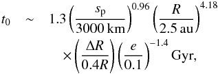 (3)where sp is the size of planetesimals, R is the radius of the planetesimal belt, and e is the eccentricity of planetesimals. Interestingly, t0 is independent of the initial number density of planetesimals (Wyatt et al. 2007). Note that the perturbation from Moon-sized or larger bodies is needed to induce the collisional fragmentation of planetesimals (Kobayasi & Löhne 2014), which is implicitly assumed in this model.
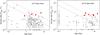 |
Fig. 5 a)Fdisk/F∗ at AKARI 18 μm versus stellar age for F-type stars. Filled circles indicate debris disk samples from previous works at 24 μm by Spitzer/MIPS (Beichman et al. 2005, 2006; Bryden et al. 2006; Chen et al. 2005a,b; Hillenbrand et al. 2008; Trilling et al. 2008). Filled squares represent excess ratios observed by AKARI at 18 μm for stars with excesses larger than 3σ (debris disk candidates), while open squares show that for all stars in our sample. The solid line indicates the evolutionary track with t0 = 0.5 Gyr, where t0 is the dissipation time scale, while the dotted line indicates evolutionary track of t0 = 2 Gyr (see text for details). b) Same as a) but for G-type stars. |
Figure 5 shows excess ratio, Fdisk/F∗, versus stellar age. We plot our samples if stellar ages are known: Estimated ages are available for four and six objects among nine F-type and seven G-type stars in Tables 3 and 4, respectively (Chen et al. 2001; Feltzing et al. 2001; Holmberg et al. 2009). We also plot the samples obtained from previous observations. The excess ratios for most of the objects are explained by the steady-state collisional cascade model (Eq. (2)) if t0< 0.5 Gyr. However at least nine objects in our sample, the ages of which are determined in the literature, can not be explained with t0< 0.5 Gyr and are rather consistent with t0 of 2 Gyr. If we assume a system like the solar system that has R ≈ 2.5 au and e ≈ 0.1, then, very large planetesimals with sp ~ 5000 km are required for t0 ~ 2 Gyr (see Eq. (3)). The bodies with sp ~ 5000 km are larger than the Mars. A small number of such large bodies can be formed but a swarm of such large bodies for collisional cascade may be unrealistic. Furthermore, there are no young objects with high fractional luminosities corresponding to t0 longer than 2 Gyr (see Fig. 5), which are progenitors of those old, bright debris disks. Therefore, those old debris disk objects with high fractional luminosity may not be explained only by the conventional steady-state cascade model.
Kennedy & Wyatt (2012) explored IR excess for Kepler objects by using the WISE catalog and indicated that large excesses around in old stars can be explained by chance alignment of interstellar dust or background galaxies. Merin et al. (2014) observed stars showing warm-IR excesses in WISE bands 3 and 4 with Herschel and obtained no detection in any of the targets, which indicates most of such excesses are likely caused by chance alignment of the foreground or background objects. Though our sample covers brighter nearby objects than the distant WISE sample, we investigate the probability of chance alignment of known extragalactic sources and/or diffuse dust emission by using NED database and the AKARI 18 μm images, respectively. No suspected features are found in these processes (see Sect. 2.7). Therefore, we judge that the stars have debris disks. High spatial resolution observations with future large telescopes might resolve the disk or reveal a nearby background source, thus clarifying the origin of the excesses.
If they are true debris disks, these high excesses around old stars may be related to other non-steady processes such as follows. (a) In planet formation, a swarm of planetesimals produces a small number of planetary embryos and the stirring by planetary embryos induces collisional fragmentation of remnant planetesimals, resulting in the formation of debris disks: Low mass disks composed of large planetesimals tend to have long timescales of disk evolution (Kobayasi & Löhne 2014), which may explain these high excess around old stars. (b) In the late stages of planet formation, giant impacts among Mars-sized planetary embryos, which produced the Moon in the solar system, occur through long-term orbital instability. Although the total mass of fragments ejected from giant impacts is much smaller than planetary embryos, the excesses ratios resulting from giant impacts increase to observable levels (Genda et al. 2015), which may form late debris disks. (c) In the solar system, the late heavy bombardment is believed to have occurred at ~ 3.9 Gyr, based on radiometric ages of impact melts of lunar samples (Tera et al. 1974). It may be related to dynamical events of planets in the solar system, which induce the formation of late debris disks in other systems (Booth et al. 2009; Fujiwara et al. 2013). (d) In planet-hosting systems, planets trap dust grains in their mean motion resonances in a long timescale (Liou et al. 1996), which may form late bright debris disks. The resonance trap is particularly studied for the Earth’s resonance orbits in the solar system by the past infrared survey missions (e.g., Kelsall et al. 1989; Rowan-Robinson & May 2013). Furthermore, the temporal variation of this component is indicated by the recent analysis of the AKARI all-sky survey data (Kondo et al. 2016), although the variability is small.
Each non-steady process leads to different temporal evolution of excess ratios. The origin of the high excess debris disks around old stars will be revealed by investigating the temporal variability of infrared excess emission via multi-epoch observations. The next chance will be brought us by the next space infrared mission, JWST or SPICA. Imaging observations with ground-based large telescopes such as TMT are also expected. The first detections of such planets are being made by ground-based direct imaging surveys, and space-based detections will follow in the future (e.g., WFIRST).
5. Summary
By using the AKARI mid-IR all-sky PSC, we have explored debris disks with 18 μm excess emission. We have carefully selected nearby isolated stars and compared their estimated photospheric fluxes with observed fluxes at a wavelength of 18 μm. For accurate estimation of the photospheric fluxes of the central stars, we have performed J, H, and Ks band photometry with IRSF for nearby bright stars whose 2MASS fluxes have large uncertainties due to saturation. The flux uncertainties of the central stars have been improved from 14% to 1.8% on average. As a result, we have successfully detected 53 debris-disk candidates out of 678 main-sequence stars. At least nine objects of them have large excess emission for their ages, which cannot be explained by the conventional steady state collisional cascade model.
Acknowledgments
This research is based on observations with AKARI, a JAXA project with the participation of ESA. The IRSF project is a collaboration between Nagoya University and the South African Astronomical Observatory (SAAO) supported by the Grants-in-Aid for Scientific Research on Priority Areas (A) (Nos. JP10147207 and JP10147214) and Optical & Near-IR Astronomy Inter-University Cooperation Program, from the Ministry of Education, Culture, Sports, Science and Technology (MEXT) of Japan and the National Research Foundation (NRF) of South Africa. This publication makes use of data products from the Two Micron All Sky Survey, which is a joint project of the University of Massachusetts and the Infrared Processing and Analysis Center/California Institute of Technology, funded by the National Aeronautics and Space Administration and the National Science Foundation. This research has made use of the NASA/IPAC Infrared Science Archive, and the NASA/IPAC Extragalactic Database (NED), which is operated by the Jet Propulsion Laboratory, California Institute of Technology, under contract with the National Aeronautics and Space Administration. This research has made use of the SIMBAD database, operated at CDS, Strasbourg, France. We thank Dr. G. Kennedy for careful reading and emendation of the manuscript. This work is supported by the Grant-in-Aid for the Scientific Research Funds (Nos. JP24740122, JP26707008, JP50377925, and JP26800110) from Japan Society for the Promotion of Science (JSPS), and (No. JP23103002) from the Ministry of Education, Culture, Sports, Science and Technology (MEXT) of Japan.
References
- Aumann, H. H., Beichman, C. A., Gillett, F. C., et al. 1984, ApJ, 278, 23 [Google Scholar]
- Benz, W., & Asphaug, E. 1999, Icarus, 142, 5 [NASA ADS] [CrossRef] [Google Scholar]
- Beichman, C. A., Bryden, G., Rieke, G. H., et al. 2005, ApJ, 622, 1160 [NASA ADS] [CrossRef] [Google Scholar]
- Beichman, C. A., Bryden, G., Stapelfeldt, K. R., et al. 2006, ApJ, 652, 1674 [NASA ADS] [CrossRef] [Google Scholar]
- Bessell, M. S., & Brett, J. M. 1988, PASP, 100, 1134 [NASA ADS] [CrossRef] [Google Scholar]
- Booth, M., Wyatt, M. C., Morbidelli, A., et al. 2009, MNRAS, 399, 385 [NASA ADS] [CrossRef] [Google Scholar]
- Bryden, G., Beichman, C. A., Trilling, D. E., et al. 2006, ApJ, 636, 1098 [NASA ADS] [CrossRef] [Google Scholar]
- Bryden, G., Beichman, C. A., Carpenter, J. M., et al. 2009, ApJ, 705, 1226 [NASA ADS] [CrossRef] [Google Scholar]
- Carter, B. S. 1990, MNRAS, 242, 1 [NASA ADS] [CrossRef] [Google Scholar]
- Chen, Y. Q., Nissen, P. E., Benoni, T., & Zhao, G. 2001, A&A, 371, 943 [NASA ADS] [CrossRef] [EDP Sciences] [Google Scholar]
- Chen, C. H., Patten, B. M., Werner, M. W., et al. 2005a, ApJ, 634, 1372 [NASA ADS] [CrossRef] [Google Scholar]
- Chen, C. H., Jura, M., Gordon, K. D., & Blaylock, M. 2005b, ApJ, 623, 493 [NASA ADS] [CrossRef] [Google Scholar]
- Clarke, A. J., Oudmaijer, R. D., & Lumsden, S. L. 2005, MNRAS, 363, 1111 [NASA ADS] [CrossRef] [Google Scholar]
- Cohen, M., Walker, R. G., Carter, B., et al. 1999, AJ, 117, 1864 [NASA ADS] [CrossRef] [Google Scholar]
- Cox, A. N. 2000, Allen’s Astrophysical Quantities, 4th edn. (Springer) [Google Scholar]
- Cutri, R. M., Skrutskie, M. F., van Dyk, S., et al. 2003, The IRSA 2MASS All-Sky Point Source Catalog, NASA/IPAC, Infrared Science Archive, http://irsa.ipac.caltech.edu/applications/Gator/ [Google Scholar]
- Dodson-Robinson, S. E., Beichman, C. A., Carpenter, J. M., & Bryden, G. 2011, AJ, 141, 11 [NASA ADS] [CrossRef] [Google Scholar]
- Ducati, J. R. 2002, Vizier Online Data Catalog: II/237 [Google Scholar]
- Eiroa, C., Marshall, J. P., Mora, A., et al. 2013, A&A, 555, A11 [NASA ADS] [CrossRef] [EDP Sciences] [Google Scholar]
- Feltzing, S., Holmberg, J., & Hurley, J. R. 2001, A&A, 377, 911 [NASA ADS] [CrossRef] [EDP Sciences] [Google Scholar]
- Fitzpatrick, L. E., & Massa, D. 2009, ApJ, 699, 1209 [NASA ADS] [CrossRef] [Google Scholar]
- Fujiwara, H., Yamashita, T., Ishihara, D., et al. 2009, ApJ, 695, L88 [NASA ADS] [CrossRef] [Google Scholar]
- Fujiwara, H., Onaka, T., Ishihara, D., et al. 2010, ApJ, 714, L152 [NASA ADS] [CrossRef] [Google Scholar]
- Fujiwara, H., Onaka, T., Takita, S., et al. 2012, ApJ, 759, L18 [NASA ADS] [CrossRef] [Google Scholar]
- Fujiwara, H., Ishihara, D., Onaka, T., et al. 2013, A&A, 550, A45 [NASA ADS] [CrossRef] [EDP Sciences] [Google Scholar]
- Genda, H., Kobayashi, H., & Kokubo, E. 2015, ApJ, 810, 2 [Google Scholar]
- Greaves, J. S., Fischer, D. A., & Wyatt, M. C. 2006, MNRAS, 366, 283 [NASA ADS] [CrossRef] [Google Scholar]
- Habing, H. J., Dominik, C., Jourdain de Muizon, M., et al. 2001, A&A, 365, 545 [NASA ADS] [CrossRef] [EDP Sciences] [Google Scholar]
- Hartmann, W. K., Ryder, G., Dones, L., & Grinspoon, D. 2000, in Origin of the Earth and Moon, eds. R. M. Canup, K. Righter et al. (Tucson, AZ: Univ. Arizona Press), 493 [Google Scholar]
- Hillenbrand, L. A., Carpenter, J. M., Kim, J. S., et al. 2008, ApJ, 677, 630 [Google Scholar]
- Holmberg, J., Nordström, B., & Andersen, J. 2009, A&A, 501, 941 [NASA ADS] [CrossRef] [EDP Sciences] [Google Scholar]
- Houk, N. 1978, Michigan Catalog of Two-dimensional Spectral Types for HD Stars, 2 (Ann Arbor: Univ. Michigan Dept. Astron.) [Google Scholar]
- Houk, N. 1982, Michigan Catalog of Two-dimensional Spectral Types for HD Stars, 3 (Ann Arbor: Univ. Michigan Dept. Astron.) [Google Scholar]
- Houk, N., & Cowley, A. P. 1975, Michigan Catalog of Two-dimensional Spectral Types for HD Stars, 1 (Ann Arbor: Univ. Michigan Dept. Astron.) [Google Scholar]
- Houk, N., & Smith-Moore, M. 1988, Michigan Catalog of Two-dimensional Spectral Types for HD Stars, 4 (Ann Arbor: Univ. Michigan Dept. Astron.) [Google Scholar]
- Houk, N., & Swift, C. 1999, Michigan Catalog of Two-dimensional Spectral Types for HD Stars, 5 (Ann Arbor: Univ. Michigan Dept. Astron.) [Google Scholar]
- Ishihara, D., Onaka, T., Kataza, H., et al. 2006, AJ, 131, 1074 [NASA ADS] [CrossRef] [Google Scholar]
- Ishihara, D., Onaka, T., Kataza, H., et al. 2010, A&A, 514, A1 [NASA ADS] [CrossRef] [EDP Sciences] [Google Scholar]
- Ishihara, D., Kaneda, H., Onaka, T., et al. 2011, A&A, 534, A79 [NASA ADS] [CrossRef] [EDP Sciences] [Google Scholar]
- Kaneda, H., Kim, W., Onaka, T., et al. 2007, PASJ, 59, 423 [CrossRef] [Google Scholar]
- Kawada, M., Baba, H., Barthel, P. D., et al. 2007, PASJ, 59, 389 [Google Scholar]
- Kelsall, T., Weiland, J. L., Franz, B. A., et al. 1989, ApJ, 508, 44 [Google Scholar]
- Kennedy, G. M., & Wyatt, M. C. 2012, MNRAS, 426, 91 [NASA ADS] [CrossRef] [Google Scholar]
- Kennedy, G. M., Murphy, S. J., Lisse, C. M., et al. 2014, MNRAS, 438, 3299 [NASA ADS] [CrossRef] [Google Scholar]
- Kobayashi, H., & Löhne, T. 2014, MNRAS, 422, 3266 [NASA ADS] [CrossRef] [Google Scholar]
- Kobayashi, H., & Tanaka, H. 2010, Icarus, 206, 735 [NASA ADS] [CrossRef] [Google Scholar]
- Kondo, T., Ishihara, D., Kaneda, H., et al. 2016, AJ, 151, 71 [NASA ADS] [CrossRef] [Google Scholar]
- Kóspál, Á., Ardila, D. R., Moór, A., Ábrahám, P. 2009, ApJ, 700, 73 [Google Scholar]
- Kurucz, R. L. 1992, in The Stellar Populations of Galaxies, eds. B. Barbuy, & A. Renzini, IAU Symp., 149, 225 [Google Scholar]
- Lallement, R., Welsh, B. Y., Vergely, J. L., Crifo, F., & Sfeir, D. 2003, A&A, 411, 447 [EDP Sciences] [Google Scholar]
- Liou, J.-C., Zook, H. A., & Dermott, S. F. 1996, Icarus, 124, 429 [NASA ADS] [CrossRef] [Google Scholar]
- Mannings, V., & Barlow, M. J. 1998, ApJ, 497, 330 [NASA ADS] [CrossRef] [Google Scholar]
- McDonald, I., Zijlstra, A. A., & Boyer, M. L. 2012, MNRAS, 427, 343 [NASA ADS] [CrossRef] [Google Scholar]
- Meng, H. Y. A., Rieke, G. H., Su, K. Y. L., et al. 2012, ApJ, 751, L17 [NASA ADS] [CrossRef] [Google Scholar]
- Meng, H. Y. A., Su, K. Y. L., Rieke, G. H., et al. 2014, Science, 345, 1032 [NASA ADS] [CrossRef] [Google Scholar]
- Merin, B., David, R. A., Alvaro, R., et al. 2014, A&A, 569, A89 [NASA ADS] [CrossRef] [EDP Sciences] [Google Scholar]
- Moro-Martín, A., Carpenter, J. M., Meyer, M. R., et al. 2007, ApJ, 658, 1312 [NASA ADS] [CrossRef] [Google Scholar]
- Moro-Martín, A., Marshall, J. P., Kennedy, G., et al. 2015, ApJ, 801, 143 [NASA ADS] [CrossRef] [Google Scholar]
- Murakami, H., Baba, H., Barthel, P., et al. 2007, PASJ, 59, 369 [Google Scholar]
- Nagayama, T., Nagashima, C., Nakajima, Y., et al. 2003, Proc. SPIE, 4841, 459 [NASA ADS] [CrossRef] [Google Scholar]
- Neugebauer, G., Habing, H. J., van Duinen, R., et al. 1984, ApJ, 278, 1 [NASA ADS] [CrossRef] [Google Scholar]
- Olofsson, J., Juhász, A., Henning, Th., et al. 2012, A&A, 542, A90 [NASA ADS] [CrossRef] [EDP Sciences] [Google Scholar]
- Onaka, T., Matsuhara, H., Wada, T., et al. 2007, PASJ, 59, 401 [NASA ADS] [Google Scholar]
- Oudmaijer, R. D., van der Veen, W. E. C. J., Waters, L. B. F. M., et al. 1992, A&AS, 96, 625 [NASA ADS] [Google Scholar]
- Patel, R., Metchev, S. A., & Heinze, A. 2014, ApJS, 212, 10 [NASA ADS] [CrossRef] [Google Scholar]
- Pei, Y. C. 1992, ApJ, 395, 130 [NASA ADS] [CrossRef] [Google Scholar]
- Perryman, M. A. C., Lindegren, L., Kovalevsky, J., et al. 1997, A&A, 323, L49 [NASA ADS] [Google Scholar]
- Planck Collaboration XIV 2014, A&A, 571, A14 [NASA ADS] [CrossRef] [EDP Sciences] [Google Scholar]
- Rhee, J. H., Song, I., Zuckerman, B., & McElwain, M. 2007, ApJ, 660, 1556 [NASA ADS] [CrossRef] [MathSciNet] [Google Scholar]
- Ribas, Á., Merín, B., Bouy, H., et al. 2013, A&A, 552, 115 [Google Scholar]
- Rieke, G. H., Su, K. Y. L., Stansberry, J. A., et al. 2005, ApJ, 620, 1010 [NASA ADS] [CrossRef] [Google Scholar]
- Rowan-Robinson, M., & May, B. 2013, MNRAS, 429, 2894 [NASA ADS] [CrossRef] [Google Scholar]
- Sato, S., Nagata, T., Kawai, T., et al. 2001, The Astronomical Herald, 94, 125 [NASA ADS] [Google Scholar]
- Schneider, A., Song, I., Melis, C., et al. 2013, ApJ, 777, 78 [NASA ADS] [CrossRef] [Google Scholar]
- Siegler, N., Muzerolle, J., Young, E. T., et al. 2007, ApJ, 654, 580 [NASA ADS] [CrossRef] [Google Scholar]
- Skrutskie, M. F., Cutri, R. M., Stiening, R., et al. 2006, AJ, 131, 1163 [NASA ADS] [CrossRef] [Google Scholar]
- Spangler, C., Sargent, A. I., Silverstone, M. D., Becklin, E. E., & Zuckerman, B. 2001, ApJ, 555, 932 [NASA ADS] [CrossRef] [Google Scholar]
- Su, K. Y. L., Rieke, G. H., & Stansberry, J. A., 2006, ApJ, 653, 675 [NASA ADS] [CrossRef] [Google Scholar]
- Thébault, P., Marzari, F., & Augereau, J.-C. 2010, A&A, 524, A13 [NASA ADS] [CrossRef] [EDP Sciences] [Google Scholar]
- Tera, F., Papanastassiou, D. A., & Wasserburg, G. J. 1974, Earth Planet. Sci. Lett., 22, 1 [NASA ADS] [CrossRef] [Google Scholar]
- Tody, D. 1986, Proc. SPIE, 627, 733 [NASA ADS] [CrossRef] [Google Scholar]
- Trilling, D. E., Bryden, G., Beichman, C. A., et al. 2008, ApJ, 674, 1086 [NASA ADS] [CrossRef] [Google Scholar]
- Weingartner, J. C., & Draine, B. T. 2001, ApJ, 548, 296 [NASA ADS] [CrossRef] [Google Scholar]
- Wright, C. O., Egan, M. P., Kraemer, K. E., & Price, S. D. 2003, AJ, 125, 359 [NASA ADS] [CrossRef] [Google Scholar]
- Wright, E. L., Peter, R. M. E., Mainzer, A. K., et al. 2010, AJ, 140, 1868 [NASA ADS] [CrossRef] [Google Scholar]
- Wyatt, M. C. 2008, ARA&A, 46, 339 [NASA ADS] [CrossRef] [Google Scholar]
- Wyatt, M. C., Smith, R., Greaves, J. S., et al. 2007, ApJ, 658, 569 [NASA ADS] [CrossRef] [Google Scholar]
Appendix A: Accurate J, H, Ks photometry of nearby bright stars
Using the IRSF telescope (Sato et al. 2001), we have performed J, H, and Ks band photometry of 325 bright stars which have large photometric uncertainties due to saturation in the 2MASS catalog (Cutri et al. 2003). IRSF is the near-infrared telescope with a φ1.4 m primary mirror located in Sutherland, South Africa at 1800 m elevation. It is managed by Nagoya University. SIRIUS (Nagayama et al. 2003) is the wide-field camera, which enables simultaneous J, H, and Ks band wide field imaging. The field-of-view (FOV) size is  . The pixel scale is
  , while the PSF size is 1′′–2′′ depending on the weather.
The observations were carried out using the ND filter for × 10-2 flux attenuation in six nights with relatively stable weather: 2011 August 6, 2011 August 9, 2012 February 5, 2012 February 10, and 2013 June 12. In the observations using ND filters, we cannot make flux calibration using standard stars in the same FOV, because, in most cases, only the target star is detected in each image. Based on the observations of bright standard stars (Carter 1990), we derive the system response (estimated flux/observed flux (count s-1)) as a function of sec(z) specific to each night and each ND filter where z is a zenith angle. A set of examples of the functions for the J-, H-, and Ks-bands in a night are shown in Fig. A.1. The system response is determined with an accuracy of 0.1–0.2%. Then we applied these functions to each observation.
Observational data are reduced with the standard pipeline for the SIRIUS data. The images are stacked and aperture photometry is employed for each target star using the IRAF phot package (Tody 1986). The parameters are optimized to maximize the signal-to-noise ratios and to obtain total fluxes of stars without an aperture correction. We adopted an aperture radius of 5′′, an annulus (the width of the gap between the source area and the sky area) of 3′′, and a sky width (the width of the annulus of the sky area) of 3′′.
Table 2 summarizes J, H, Ks photometric results for our target stars. Figure A.2 compares the IRSF J, H, Ks fluxes with the 2MASS J, H, Ks fluxes for the same stars. Our IRSF measurements are statistically consistent with the 2MASS measurements within the uncertainties. The error bars along the horizontal axis are systematically longer than those along the vertical axis, indicating that the IRSF measurements have smaller uncertainties than the 2MASS measurements. The relations between the flux and flux errors are shown in Fig. 1. The averaged flux errors are reduced from 17%, 14%, and 11% to 1.9%, 1.4%, and 2.0%, for the J, H, and Ks band, respectively. In Fig. A.3, we compare the color−color diagram based on the 2MASS photometry and that based on the IRSF photometry. While the 2MASS measurements show a large scatter, our IRSF measurements trace the intrinsic locus of main-sequence stars (Bessell & Brett 1988). This confirms the reliability of the IRSF measurements.
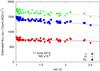 |
Fig. A.1 Ratio of the estimated fluxes over the observed fluxes of standard stars as a function of sec(z). This example is of the observation on 11th June 2013. This plot is made for every night for every ND filters. The circle, triangle, and square indicate the J, H, and Ks bands, respectively. The solid line, the dotted line, and the dot-dashed line indicate fitting results for the J, H, and Ks bands, respectively. |
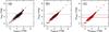 |
Fig. A.2 IRSF photometry versus 2MASS photometry for our sample of 325 bright main-sequence stars in the J band (a), H band (b), and Ks band (c). |
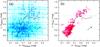 |
Fig. A.3 a) J−H versus H−Ks color−color diagram of bright main-sequence stars based on the 2MASS measurements. The solid curve indicates locus of main-sequence stars while the dotted curve indicates that of giant stars (Bessell & Brett 1988). The solid arrow shows the interstellar extinction vector for Av = 1 mag, using the Weingartner & Draine (2001) Milky Way model of Rv = 3.1. b) Same as a), but for the IRSF measurements. The objects above dashed lines are removed from our main-sequence sample because they might be giant stars. |
Appendix B: Reliability of the fitting of photospheric emission
For the evaluation of the fitting results in the estimation of photospheric emission, we compare the output parameters (Teff and S) with the related parameters quoted from the literature (spectral type and distance). Figure B.1a shows Teff versus spectral type and Fig. B.1b shows S versus distance-2 for our sample. All the objects are aligned along the intrinsic locus of main-sequence stars in both plots. These indicate that our sample selection and fitting process work well in general.
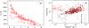 |
Fig. B.1 a) Effective temperature of a central star (fitting result) versus spectral type from the literature (Wright et al. 2003). b) Scale factor S (fitting result) versus reciprocal of the square of the distance from the Hipparcos catalog (Perryman et al. 1997). |
Appendix C: Uncertainties in SED fitting of photosphere using pre-computed grids
In estimating 18 μm photospheric emission of stars by fitting their optical-to-near-infrared SEDs with the Kurucz model (Kurucz 1992), we use the pre-computed grids for Teff, log (g), and metallicity. By using these quantized parameters to the fitting, the uncertainty for Teff is certainly increased. But its effect is small for the predicted F∗ at 18 μm. It is much smaller than the total systematic error considered in the excess identification: 0.126 for AKARI–IRSF sample and 0.182 for AKARI–2MASS sample (see Sect. 2.7). This is because the change in Teff affects spectra in shorter wavelengths (< 1μm) and less affects longer wavelengths.
Figure C.1 shows an example of χ2 versus Teff plot for the SED fitting of the star (HD 187748). The Teff range which satisfies 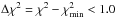 is 6140–6760 K, which is the 68.3% confidence range assuming the normal distribution, and thus 1σ equivalent uncertainties. If the sampling against Teff is finer, χ2 at the true Teff might be smaller, and the Teff for 1σ is smaller. However, the uncertainty in the estimate of Fstar is small enough even in this Teff range (0.4% for this sample). We estimate uncertainties in Teff and F∗ for each star in this method. Figure C.2 shows the distribution of the 1σ uncertainties in the photospheric fitting for all the stars in our sample. The uncertainties in the fitting process are much smaller than the total systematic error considered in the excess identification. Thus deviation of Teff does not significantly affect the prediction of F∗.
It should be noted that the fitting result of Teff for earlier type stars tends to be different from the value expected from the spectral type. The Teff for HD 75416 (B8), HD 161840 (B8), and HD 222173 (B8) result in 15 000 K, the maximum value in the fitting range. They do not show a convincing χ2 curve and an asymptotic trend to the value of 15 000 K. It might because the peak of the photospheric SED is shorter than the wavelengths of input data. The Teff for HD 279128 (B8), HD 146055 (B9) result in 6000 K and 7000 K, respectively. It might be due to the constraint in AV in addition to the large 2MASS photometric errors. However, they do not affect the excess identification because all of them show apparent mid-IR excess in Fig. 3.
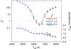 |
Fig. C.1 χ2 versus Teff in the fitting photospheric emission for HD 187748 as an example (left axis). Red, green, and blue points indicate cases for log (g) = 4.0, 4.5, and 5.0, respectively. Deviation of F∗ ,18 around the best-fit value (F∗ ,18 at Teff = 6500, log (g) = 4.0), is also overlaid in this plot (right axis). |
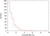 |
Fig. C.2 Distribution of uncertainties in the photospheric fitting process. |
Appendix D: Point image analysis for debris-disk candidates
We have investigated the images in 2MASS Ks-band, and AKARI 9 μm, as well as those in AKARI 18 μm for all the 53 debris-disk candidates to check image artifacts and contamination of other sources. Figure D.1 shows these images. In previous work looking for WISE infrared excesses around faint stars contamination and artifacts have posed problems (Kennedy & Wyatt 2012; Ribas et al. 2013). However, the fluxes of our debris-disk candidates are at the brightest end of WISE dynamic range.
AKARI has better spatial resolution than WISE. Thus, the AKARI images less suffer confusion than the WISE data. In the AKARI 18 μm images, effects of image artifacts were not found and contaminating sources were not recognized. For example, HD 34890, HD 102323, and HD 165014 are accompanied by closely located sources in the line of sight, but they are clearly separated in the AKARI 18 μm image. Therefore, we conclude that spurious detections are not among our debris-disk candidates.
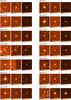 |
Fig. D.1 2MASS Ks, AKARI 9 μm, and AKARI 18 μm images (from left to right) for 53 debris disks candidates. |
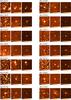 |
Fig. D.1 continued. |
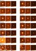 |
Fig. D.1 continued. |
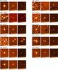 |
Fig. D.1 continued. |
Appendix E: Collisional evolution
In a quasi steady-state collisional cascade, the flux-ratio evolution is given by (e.g., Kobayashi & Tanaka 2010), 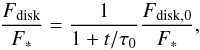 (E.1)where Fdisk,0 is the initial disk flux and τ0 is the initial collisional cascade timescale, given by Kobayashi & Tanaka (2010) as,
 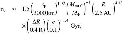 (E.2)where sp is the planetesimal radius, the radius of largest bodies in the collisional cascade, Mtot,0 is the initial total mass of bodies, M⊕ is the mass of the Earth, R is the radius of the planetesimal belt, ΔR is the width of the belt, and e is the eccentricity of planetesimals. For the derivation of Eq. (E.1), a steady-state collisional cascade is assumed. The steady state is achieved at t ≫ τ0 and the flux ratio depends on the initial condition at t ≪ τ0. Therefore we additionally assume t ≫ τ0 and then Eq. (E.1) becomes
 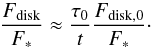 (E.3)In the steady-state collisional cascade, the surface number density of bodies with radii from s to s + ds, ns(s)ds, is proportional to s1−p, where p is a constant. The power-law index p is determined by the dependence of collisional velocity and collisional strength on the radii of bodies (Kobayashi & Tanaka 2010). The collisional strength is governed mainly by material properties
for s ≲ 1 km and by gravity s ≳ 1 km (e.g., Benz & Asphaug 1999). According to Kobayashi & Tanaka (2010) based on the mass dependence of strength obtained by hydrodynamic simulations (Benz & Asphaug 1999), we assume p ≈ 3.66 for s< 1 km and p ≈ 3.04 for s> 1 km. The radius of smallest bodies is set to be 1 μm. For blackbody dust, this size distribution gives 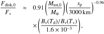 (E.4)where Bν is the Planck function, T∗ and Td are the stellar and dust temperatures, respectively, the value of Bν(T∗) /Bν(Td) is estimated for Td = 180 K, T∗ = 5800 K, and ν for the wavelength of 18 μm, and we assume that sp ≫ 1 km for this derivation. From Eqs. (E.2)–(E.4), we obtain Eq. (3). As shown in Eq. (3), t0 is independent of the total mass of bodies and the width of the planetesimal belt.
Appendix F: Additional figure
 |
Fig. F.1 Optical to mid-IR SEDs of our debris-disk candidates with 18 μm excess emission. Crosses, open squares, filled squares, open circles, filled circles, and triangles indicate the photometric data points measured with Hipparcos (VT, BT) and USNO-B (I, z), 2MASS (J, H, Ks), IRSF (J, H, Ks), AKARI 9 μm, AKARI 18 μm, and WISE (3.4, 4.6, 12, 22 μm), respectively. The red filled circles indicate AKARI 18 μm flux used for excess identification. Solid curves indicate the contribution of the photosphere estimated on the basis of the optical to near-IR fluxes of the objects. |
 |
Fig. F.1 continued. |
All Tables
List of debris-disk candidates with the AKARI 18 μm excess emission (the 2MASS based sample).
List of debris-disk candidates with AKARI 18 μm excess emission (the IRSF based sample).
Statistics of debris-disk candidates with significant detection of the AKARI 18 μm excess emission.
All Figures
|
Fig. 1 Measurement errors from 2MASS (squares) and IRSF (crosses) as a function of the magnitude in the a) J band, b) H band, and c) Ks band. |
| In the text | |
|
Fig. 2 a) Distributions of the excess ratio ((F18,obs−F18, ∗) /F18, ∗) for our sample with IRSF measurements. The center of the peak, μ, and the standard deviation, σ, of the Gaussian distribution are indicated in the graphs. b) Same as a), but for the sample with 2MASS measurements. |
| In the text | |
|
Fig. 3 Flux ratio (Fdisk/F∗) in the previous works plotted against the flux ratio (for the AKARI 18 μm) in this work for the same stars. The filled circles, open circles, filled squares, filled diamonds, pluses, crosses, open triangles, and open squares indicate the flux ratios for the AKARI 18 μm data by Fujiwara et al. (2013), those by McDonald et al. (2012), the WISE 22 μm data by McDonald et al. (2012), the IRAS 25 μm data by McDonald et al. (2012), the Spitzer/MIPS 24 μm data by Su et al. (2006), those by Rieke et al. (2005), those by Trilling et al. (2008), and those by Bryden et al. (2006), respectively. For reference, the red, orange, yellow, green, and blue lines indicate locations in this plot when the disk emission is the blackbody with T = 800, 400, 200, 100, and 50 K, respectively. The dashed lines correspond to the Spitzer 24 μm flux, and dash-dot-dashed lines correspond to the WISE 22 μm flux. |
| In the text | |
|
Fig. 4 Distance plotted as a function of the spectral type for our sample. The open circles indicate all the 678 sample. The filled circles and filled boxes indicate the debris-disk candidates with the IRSF and 2MASS measurements, respectively. The dotted curve indicates the detection limit for objects without IR excess according to our definition. |
| In the text | |
|
Fig. 5 a)Fdisk/F∗ at AKARI 18 μm versus stellar age for F-type stars. Filled circles indicate debris disk samples from previous works at 24 μm by Spitzer/MIPS (Beichman et al. 2005, 2006; Bryden et al. 2006; Chen et al. 2005a,b; Hillenbrand et al. 2008; Trilling et al. 2008). Filled squares represent excess ratios observed by AKARI at 18 μm for stars with excesses larger than 3σ (debris disk candidates), while open squares show that for all stars in our sample. The solid line indicates the evolutionary track with t0 = 0.5 Gyr, where t0 is the dissipation time scale, while the dotted line indicates evolutionary track of t0 = 2 Gyr (see text for details). b) Same as a) but for G-type stars. |
| In the text | |
|
Fig. A.1 Ratio of the estimated fluxes over the observed fluxes of standard stars as a function of sec(z). This example is of the observation on 11th June 2013. This plot is made for every night for every ND filters. The circle, triangle, and square indicate the J, H, and Ks bands, respectively. The solid line, the dotted line, and the dot-dashed line indicate fitting results for the J, H, and Ks bands, respectively. |
| In the text | |
|
Fig. A.2 IRSF photometry versus 2MASS photometry for our sample of 325 bright main-sequence stars in the J band (a), H band (b), and Ks band (c). |
| In the text | |
|
Fig. A.3 a) J−H versus H−Ks color−color diagram of bright main-sequence stars based on the 2MASS measurements. The solid curve indicates locus of main-sequence stars while the dotted curve indicates that of giant stars (Bessell & Brett 1988). The solid arrow shows the interstellar extinction vector for Av = 1 mag, using the Weingartner & Draine (2001) Milky Way model of Rv = 3.1. b) Same as a), but for the IRSF measurements. The objects above dashed lines are removed from our main-sequence sample because they might be giant stars. |
| In the text | |
|
Fig. B.1 a) Effective temperature of a central star (fitting result) versus spectral type from the literature (Wright et al. 2003). b) Scale factor S (fitting result) versus reciprocal of the square of the distance from the Hipparcos catalog (Perryman et al. 1997). |
| In the text | |
|
Fig. C.1 χ2 versus Teff in the fitting photospheric emission for HD 187748 as an example (left axis). Red, green, and blue points indicate cases for log (g) = 4.0, 4.5, and 5.0, respectively. Deviation of F∗ ,18 around the best-fit value (F∗ ,18 at Teff = 6500, log (g) = 4.0), is also overlaid in this plot (right axis). |
| In the text | |
|
Fig. C.2 Distribution of uncertainties in the photospheric fitting process. |
| In the text | |
|
Fig. D.1 2MASS Ks, AKARI 9 μm, and AKARI 18 μm images (from left to right) for 53 debris disks candidates. |
| In the text | |
|
Fig. D.1 continued. |
| In the text | |
|
Fig. D.1 continued. |
| In the text | |
|
Fig. D.1 continued. |
| In the text | |
|
Fig. F.1 Optical to mid-IR SEDs of our debris-disk candidates with 18 μm excess emission. Crosses, open squares, filled squares, open circles, filled circles, and triangles indicate the photometric data points measured with Hipparcos (VT, BT) and USNO-B (I, z), 2MASS (J, H, Ks), IRSF (J, H, Ks), AKARI 9 μm, AKARI 18 μm, and WISE (3.4, 4.6, 12, 22 μm), respectively. The red filled circles indicate AKARI 18 μm flux used for excess identification. Solid curves indicate the contribution of the photosphere estimated on the basis of the optical to near-IR fluxes of the objects. |
| In the text | |
|
Fig. F.1 continued. |
| In the text | |
Current usage metrics show cumulative count of Article Views (full-text article views including HTML views, PDF and ePub downloads, according to the available data) and Abstracts Views on Vision4Press platform.
Data correspond to usage on the plateform after 2015. The current usage metrics is available 48-96 hours after online publication and is updated daily on week days.
Initial download of the metrics may take a while.