| Issue |
A&A
Volume 600, April 2017
|
|
|---|---|---|
| Article Number | A4 | |
| Number of page(s) | 10 | |
| Section | Interstellar and circumstellar matter | |
| DOI | https://doi.org/10.1051/0004-6361/201630101 | |
| Published online | 17 March 2017 | |
Structure and dynamics of the molecular gas in M 2–9: a follow-up study with ALMA⋆
1 Institut de Radioastronomie Millimétrique, 300 rue de la Piscine, 38406 Saint-Martin-d’Hères France
e-mail: This email address is being protected from spambots. You need JavaScript enabled to view it.
2 Observatorio Astronómico Nacional, Ap 112, 28803 Alcalá de Henares, Spain
e-mail: This email address is being protected from spambots. You need JavaScript enabled to view it.
3 Observatorio Astronómico Nacional, Alfonso XII No. 3, 28014 Madrid, Spain
4 Centro de Astrobiología (CSIC-INTA), ESAC, Camino Bajo del Castillo s/n, Urb. Villafranca del Castillo, 28691 Villanueva de la Cañada, Madrid, Spain
5 Instituto de Ciencia de Materiales de Madrid (CSIC), 28049 Madrid, Spain
6 Joint ALMA Observatory (JAO) and European Southern Observatory, Alonso de Cordova 3107, Vitacura, Casilla 19001, Santiago, Chile
Received: 21 November 2016
Accepted: 13 January 2017
Abstract
Context. M 2–9 is a young planetary nebula (PN) that shows the characteristics of its last ejections in unprecedented detail. These last ejections are thought to trigger the post−asymptotic giant branch evolution.
Aims. To assemble an overall picture of how M 2–9 was shaped, we analyzed the characteristics of the different molecular gas components and their relation with the warmer parts of the nebula that are visible in the optical domain.
Methods. 12CO and 13CO J = 3−2 line emission maps were obtained with the Atacama Large Millimeter/submillimeter Array with high angular-resolution and sensitivity.
Results. Two equatorial rings are found to host most of the cold molecular gas in M 2–9, as has been described for previous 12CO J = 2−1 emission observations. In addition, we have detected a double crown-shaped structure that is symmetric with respect to the main nebular axis, which is located 1.5′′ away from both sides of the equatorial plane. Their distribution and kinematics show a very close relationship with the inner molecular ring: both are part of the same small hourglass structure formed ~900 yr ago. Two clearly distinct ejections with a remarkable axial symmetry are found to have shaped the molecular gas distribution in M 2–9, in agreement with the ejection processes that were probably responsible for the optical lobes. For the first time, the physical conditions of the different molecular components in M 2–9 are comprehensively analyzed with a radiative transfer model. They are found to follow standard laws, like those obtained in other young PN, with densities and temperatures decreasing with radius and ballistic expansion. A total mass of ~5 × 10⁻³M⊙ was derived for the detected molecular component, the larger and older equatorial ring hosting most (~90%) of this gas.
Key words: circumstellar matter / stars: AGB and post-AGB / radio lines: stars / stars: mass-loss / stars: individual: PN M2 / 9
The reduced datacube (FITS file) is only available at the CDS via anonymous ftp to cdsarc.u-strasbg.fr (130.79.128.5) or via http://cdsarc.u-strasbg.fr/viz-bin/qcat?J/A+A/600/A4
© ESO, 2017
1. Introduction
The onset of bipolar mass ejections is believed to mark the end of the asymptotic giant branch (AGB) phase and the beginning of the fast transition to the planetary nebula (PN) stage (in ~1000 yr). Collimated post-AGB jets are thought to interact with the previously ejected AGB envelopes to shape strongly axisymmetric nebulae (Sahai et al. 2007; Balick & Frank 2002). A mechanism that is usually postulated to explain the launching of axial ejections is linked to the presence of binary stellar systems at the nebular center (Soker 2001; Frank & Blackman 2004; De Marco 2009).
M 2–9 (also known as Minkowski’s Butterfly Nebula) is a young PN with a very elongated bipolar structure (120′′× 12′′; see Schwarz et al. 1997). Two coaxial thin outflows are seen in the optical (Balick et al. 1997), the equatorial region being best probed in molecular line emission (Zweigle et al. 1997). A sequence of observations of ionized gas emission obtained every 2−5 yr shows a rotating ionizing/exciting beam from the stellar system that illuminates a line of knots with mirror symmetry in both lobes (Doyle et al. 2000; Corradi et al. 2011). These observations were the first evidence of a binary stellar system at the center that includes a post-AGB star and orbits with a period of ~90 yr (Schmeja & Kimeswenger 2001; Smith & Gehrz 2005; Livio & Soker 2001). We note that the direct detection of stellar companions still remains an observational challenge (Hrivnak et al. 2011).
Subarcsecond angular-resolution observations of 12CO J = 2−1 line emission with the Plateau de Bure interferometer (current NOEMA observatory) revealed two ring-like structures in the equatorial plane (Castro-Carrizo et al. 2012). These rings seem to be the equatorial counterparts of the two coaxial bipolar outflows seen in the optical. They expand much more slowly than standard AGB winds, at ~8 km s-1 and ~4 km s-1, respectively. Their centers were found to be offset by ~0.3′′, their systemic velocities differ by ~0.6 km s-1, and they were formed by different mass-loss episodes that occurred 1400 and 900 yr ago. To explain these characteristics, Castro-Carrizo et al. (2012) proposed that the two ejections occurred at different points along the orbit of the post-AGB (primary) star in the binary stellar system, and hence they move in different directions. These are therefore further evidence of a binary stellar system at the center. With this interpretation and the detection of differences in the measured position-velocity gradients in the different parts of the ring, Castro-Carrizo et al. (2012) estimated some characteristics of the ejections and of the binary that triggered them. A modest mass (~0.2 M⊙) was proposed for the companion of a mass-losing AGB/post-AGB primary. We note that if we could confirm that such small companion can explain the shaping of the large outflows in M 2–9, this would have important consequences for our understanding of the mechanisms that drive the shaping of asymmetrical PN.
Recently, a review of the kinematics of the optical lobes performed by Clyne et al. (2015) confirmed that these lobes were formed at the same time as the molecular equatorial rings.
In this paper we present new observations of CO low-J transitions with yet higher angular-resolution and sensitivity in order to probe these outflows in more detail and hence to review the conclusions from first data by Castro-Carrizo et al. (2012).
To avoid confusion, we note that the speeds directly measured in these data are local standard of rest (LSR) radial velocities (to which we refer as LSR velocities, or VLSR). For M 2–9 VLSR = VBSR + 14.74 km s-1, where BSR refers to the solar system barycenter standard of rest, that is, close to the heliocetric frame.
2. Observations and data reduction
Observations of the 12CO J = 3−2 (345.796 GHz) and 13CO J = 3−2 (330.588 GHz) line emission were carried out with the Atacama Large Millimeter/submillimeter Array (ALMA; project code 2013.1.00458.S). Two tracks were obtained with ALMA band-7 on June 27 and 28, 2015, with an array of 42 antennas that provided visibilities with baselines ranging between 32 and 1562 m. Observations were performed for a total of ~104 min on source. The data were first calibrated with the CASA software package. The quasar J1733-1304 was used to calibrate bandpass and gains in the two tracks, Ceres and Pallas to set the absolute flux (using the Butler-JPL-Horizons 2012 brightness models as reference). From this amplitude calibration, a flux of 1.1 Jy and 1.3 Jy was derived for the two consecutive days in J1733-1304 at the reference frequency. The difference observed in the source continuum flux between the two observations is much smaller, however, and seems in good agreement with former data (see discussion in Sect. 5).
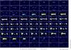 |
Fig. 1 Channel maps of the 12CO J = 3−2 line emission toward M 2–9. The center is given by the position of compact continuum emission, here subtracted, at J2000 coordinates RA = 17:05:37.966, Dec = −10:08:32.63. The LSR velocities are specified in the top left corner of each panel. Contours are shown from 4 ×σ with a spacing of 15 ×σ (where the root-mean-square noise is 2 mJy beam-1, which corresponds to 0.66 K in Rayleigh-Jeans-equivalent TMB units) as a white solid line, and at −4 ×σ as dashed red lines. The synthesized beam is 0.̋19 × 0.̋16 with the major axis PA = 116°, and is drawn in the bottom right corner of the last panel. More details can be found in Sect. 3. |
 |
Fig. 2 In contours, one over three 12CO J = 3−2 channel maps are presented with 8 km s-1 channel spacing, overlaid on the HST [NII] image published by Clyne et al. (2015) in color scale. As in Fig. 1, we detect some emission in between that from the inner ring and the crown-shaped structures. Contours are shown from 4 ×σ with a spacing of 15 ×σ (for σ = 1.5 mJy beam-1 = 0.32 K) as a solid line, and at −4 ×σ as dashed gray lines. The synthesized beam is 0.̋26 × 0.̋19 in size with the major axis PA = −18°. |
Phase-selfcalibration was later performed on visibilities with the GILDAS software package by using the compact continuum emission as reference. All of the following analysis was carried out with this package.
3. 12CO J = 3–2 data
12CO J = 3−2 channel maps are presented in Fig. 1 with a spectral spacing of 0.488 MHz (0.423 km s-1), although a detailed data inspection was performed at 0.244 MHz (0.212 km s-1) resolution. The brightness is presented in Jy beam-1 units, and the conversion factor into Rayleigh-Jeans-equivalent TMB units is 330 K/(Jy beam-1). We note that line-free continuum emission was subtracted in these channel maps. The center of all the figures we present here is indicated with a cross at J2000 coordinates RA = 17:05:37.966, Dec = −10:08:32.63, which marks the peak of the compact continuum emission (see Sect. 5). In Fig. 2 channel maps are shown with tapering (i.e., overweighting of the visibilities with shortest baselines) to increase the signal-to-noise ratio and compare the weakest emission with the optical HST image1 (available in the Hubble Legacy Archive 2013) published by Clyne et al. (2015).
Figure 3 presents the velocity-integrated 12CO J = 3−2 line emission. The emission from approaching gas is shown in blue color scale, and the emission from the receding components is shown below in orange scale. These CO-emission integrated components are also superimposed on the optical image. Astrometry was performed by using 2MASS J17053739-1008293 as reference in the optical field to properly overlay millimetric and optical data.
Two equatorial rings perpendicular to the optical lobes have previously been identified in 12CO J = 2−1 emission (Castro-Carrizo et al. 2012). They were interpreted to be the equatorial counterparts of the outer and inner optical lobes, respectively. Here we confirm the presence of the two rings and analyze their characteristics with better sensitivity and angular resolution. In addition, we detect for the first time a gas component separated from the equatorial plane and symmetric with respect to the main nebular axis (see contours in the right plot in Fig. 3). In the integrated-emission presentation (left plot in Fig. 3) we show that the clumps are parts of two crown-shaped distributions detected at a distance between ~0.4 and 2.0′′ northward and southward in the sky plane from the nebular equatorial axis (i.e., from Dec−offset = 0). This means that the molecular gas also extends throughout the main nebula lobes, at least in these two crown-shaped structures. In addition, they seem to correspond to small fractions of an hourglass-like structure. We have increased the sensitivity in our maps by overweighting the visibilities with shortest baselines (i.e., by tapering before the imaging synthesis, see Fig. 2). In this way, we have been able to detect some emission in between the crowns and the inner ring (see Fig. 2), which confirms they are both part of the same hourglass structure. This small hourglass structure has a counterpart in visible light, shown for the first time by Clyne et al. (2015, see right plot of Fig. 3.
By checking the central channels, for instance that at the systemic LSR velocity of the rings (between 80–81 km s-1, see, e.g., the right plot in Fig. 3), we see that the eastward part of the outermost ring is more separated from the center (i.e., the continuum peak) than the westward part, and that it is considerably larger (~1.3′′ instead of 1′′) and reaches a region that is outside the outermost optical lobe (for the eastermost component). Moreover, the emission detected in the largest ring significantly flares in its outermost part, this effect is again notable for the eastward side. This flaring shape already suggests an actual close relation between this dense equatorial torus and the hourglass-like axial structure seen in visible light. Finally, its brightness is found to mostly decrease with radius in 12CO J = 3−2 emission (see Fig. 1).
The small equatorial ring seems to be less complex than the large ring, however, and it is also rather well centered with respect to the continuum emission. The brightness measured along its distribution is higher than what we measure in the larger ring. We measure a deprojected radius of ~1.1′′ and a width of ~0.4′′ for a distribution that presents a good circular symmetry (see Sect. 6). In the central channels (from 81.24 to 79.97 km s-1) we see small differences in brightness between the two sides of the smaller ring, which are not significant in the integrated brightness representation (Fig. 4).
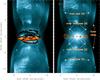 |
Fig. 3 Left: velocity-integrated 12CO J = 2−1 line emission in color scale (blue scale for the 68–80.3 km s-1 spectral range and orange for the 80.3–94 km s-1 interval) superimposed on the optical image obtained with the Hubble Space Telescope (Hubble Legacy Archive 2013). More details can be found in Sect. 3 and Fig. 1. Right: brightness 12CO J = 3−2 emission at the central velocity (LSR velocity 80.4 km s-1, after integrating in 0.4 km s-1) in contours overlaid on the optical image in color scale. Contours are plotted at 4 ×σ, and from 10 ×σ every 10 ×σ. The synthesized beam is shown in the right bottom corner of both plots. Labels are given to each of the main components identified in the optical image, which are discussed in Sect. 8. |
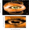 |
Fig. 4 Velocity-integrated 12CO J = 3−2 line emission, similar to that shown in Fig. 3 left. At the center, the continuum peak emission is represented by a red contour, which probably traces the position of the stellar system (see Sect. 5). Above, the data are presented in a box of 8.8′′× 4.8′′ in size, and 4.0′′× 2.2′′ in the plot below. Ellipses are plotted to help visualize the departures from symmetry, and the synthesized beam is shown in the right bottom corner of both plots. More details in Sects. 3 and 6. |
A dedicated analysis of the spatio-kinematics of the two rings is made in Sect. 6.
The peak of the global brightness distribution in the channel maps is in the inner ring, at ~0.18 Jy beam-1 in the central channels. The brightness in the innermost part of the larger ring is ~20% weaker than in the inner ring, and it radially decreases almost linearly until the outermost rim (60% weaker than the peak).
From the analysis made by Castro-Carrizo et al. (2012) and from the similar gas distribution detected in 12CO J = 3−2 emission, we can deduce that no significant flux was filtered out in the current J = 3−2 interferometric data. We also compared the total integrated flux in the 12CO J = 3−2 maps with some (poor) profiles obtained from two different single−dish telescopes (see Fig. 5, those from APEX are available through its data archive2). The good match between the absolute fluxes and the shape of the different profiles confirm that no significant flux is filtered out from the rings. It is less clear, however, whether some flux could have been filtered out between ~87−95 km s-1 LSR velocities, which would correspond to the redshifted emission from the crown-shaped structures.
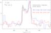 |
Fig. 5 Total integrated 12CO J = 3−2 emission compared with single-dish line profiles obtained with the 30 m IRAM and the APEX telescopes (see Sect. 3). |
Finally, we note that at LSR velocities between 82 and 84 km s-1 we tentatively detect a new component ~0.05′′ westward in the 12CO J = 3−2 emission (marked with a red arrow in Fig. 1). New data are necessary to confirm this feature, however.
4. 13CO J = 3–2 data
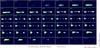 |
Fig. 6 Channel maps of the 13CO J = 3−2 line emission toward M 2–9. The center is given by the position of the compact continuum emission, here subtracted, at J2000 coordinates RA = 17:05:37.966, Dec = −10:08:32.63. The LSR velocities are specified in the top left corner of each panel. Contours are shown in 4 ×σ with a spacing of 7 ×σ (where the root-mean-square noise is 2.5 mJy beam-1, which corresponds to 0.82 K in Rayleigh-Jeans-equivalent TMB units) as a white solid line, and at −4 ×σ as dashed red lines. The synthesized beam is 0.̋20 × 0.̋17 with the major axis PA = −79° and is drawn in the bottom right corner of the last panel. |
In Fig. 6 we present channel velocity maps of the 13CO J = 3−2 line (continuum-subtracted) emission in M 2–9 with a spacing of 0.488 MHz (0.442 km s-1). The brightness is presented in Jy beam-1 units, and the conversion factor to Rayleigh-Jeans-equivalent TMB units is 326 K/(Jy beam-1). The cross at the center of the maps marks the peak of the compact continuum emission (see Sect. 5).
The distribution of the 13CO J = 3−2 emission globally coincides with that of 12CO for the two equatorial rings, and no other emission is detected along the nebula optical lobes. The 13CO J = 3−2 brightness is lower than that of 12CO: ~1.5 times weaker for the mean brightness in the outermost ring, and ~3 times lower for the inner rim of the outermost ring and for the innermost ring. We note that these moderate differences in the brightness ratio between the two isotopes can be well explained by opacity considerations (see modeling in Sect. 7).
In Fig. 7 we present the integrated spectra for the whole 12CO and 13CO J = 3−2 line emission (in black solid line), and also for that from the inner ring (in red). The weak redshifted wing seen in the 12CO profile from ~87 to 95 km s-1 comes from the molecular emission detected along the optical lobes, in the shape of a crown, which expands slightly faster than the equatorial rings. Its kinematics is analyzed in Sect. 6 and can be visualized in the simple model that best fits the data (see Sect. 7). No counterpart of the 12CO J = 3−2 crown-shaped distributions is detected in the 13CO emission. We note that this non-detection is compatible with the noise level and the observed 13CO/12CO brightness ratio. Our modeling described in Sect. 7 predicts that any 13CO emission from the crown-shaped structures should only be detectable from ~2 mJy beam-1 level, that is, below the detection threshold in the 13CO maps.
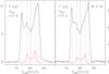 |
Fig. 7 Total integrated 12CO and 13CO J = 3−2 emission in M 2–9 is shown in black, the emission integrated over the smaller ring is presented in red. Vertical red dotted lines are plotted at LSR velocities 80.65 (inner ring Vsys), 77.65, and 83.65 km s-1, and blue dotted lines at 80 (outer ring Vsys), 74, and 86 km s-1. |
5. 0.8 mm continuum
Simultaneously to the two spectral windows in which we observed the two lines presented in Sects. 3 and 4, two additional windows of 1.9 GHz were used to map the continuum emission. After spectral verification of the continuum and line subtraction when needed, we obtained the map shown in Fig. 8 with appropriate tapering to overweight short baselines and increase sensitivity. Most of the continuum emission is found to be compact (down to 1 mJy beam-1 brightness level), unresolved, with a central peak at 0.29 Jy beam-1 located at the center. In addition, our data suggest that we have also detected an elongated structure, at 0.4−1 mJy beam-1 level, that seems to be spatially coincident with the inner ring seen in molecular emission. This new component could be coming from thermal dust emission in the inner ring environment (see Fig. 8). By fitting the data in the uv-plane we deduce that the main detected compact component is unresolved (≲0.06′′), emits a total integrated brightness of 300 ± 1 mJy, and is centered at RA = 17:05:37.966 and Dec = −10:08:32.63. In addition, we deduce an eliptical disk with 20 ± 2 mJy. We note that we measure a total integrated flux of 330 ± 2 mJy for the detected emission in the image plane.
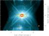 |
Fig. 8 Continuum emission in contours overlaid on the optical HST image (Hubble Legacy Archive 2013) in M 2–9. Contours are shown at 4, 8, and 12σ and from then on with a spacing of 12σ (where the root-mean-square noise is 0.1 mJy beam-1) as a solid line and at −4σ as a dashed line. The synthesized beam is 0.̋27 × 0.̋23 with the major axis PA = 122° and is drawn in the bottom right corner of the last panel. The ellipses delimiting the rims of the inner ring in Fig. 3 are also plotted here, centered at [+0.̋03, −0.̋03] according to the analysis in Sect. 6. |
The obtained value is in agreement with the 240 mJy flux measured at 230 GHz (Castro-Carrizo et al. 2012), although in both measurements we have maximum uncertainties ~10% triggered by calibration. We also note that these values may mostly be underestimated because flux is filtered out from extended emission. This is suggested by the data obtained with SCUBA by Di Francesco et al. (2008, only available online), who measured an intensity peak of 0.610 Jy beam-1 at 350 GHz for an emitting region of ~24′′ (with uncertainties of ~20% in both values).
Several components are expected to contribute to the continuum emission in M 2–9. At this frequency, Sánchez Contreras et al. (1998) deduced that the central compact continuum emission mostly originates from a region of warm (~85 K) dust close to the stellar system, and a more modest contribution from colder dust (~10 K). However, there are large uncertainties and differences between the existing measurements. In view of the existing data and models, we cannot discard the presence of a more significant component of free-free emission in the detected continuum, which could come from a very compact HII region around the stellar system and also from ionized gas from inner winds. Time variability cannot be discarded either for some free-free emission components (Sánchez Contreras et al., in prep.). Future observations at 650 GHz will provide additional information to constrain the nature of the emission here detected. In any case, we note that a stellar system of ~20 AU (as usually assumed, i.e., ~0.03′′) would be ~50 times smaller than the angular resolution achieved in these data. At higher frequencies, at wavelengths between 2−20 μm, a dusty disc of ~0.04′′ was deduced by Lykou et al. (2011) at the nebular center, which would host a very small amount of mass (~10-5M⊙).
6. Spatio-kinematic distribution
With the higher sensitivity and angular resolution of the current data with respect to previous data (Castro-Carrizo et al. 2012), we can analyze the spatio-kinematical distribution of the gas in both rings in more detail. When we fit the integrated brightness distribution with ellipses (see Fig. 4), we can roughly determine some characteristics of the rings. (1) We deduce that the inner ring has a simple morphology, elliptical in this projected image, the ring width being just slightly larger in its innermost northern approaching rim (marked with a green arrow in Fig. 4). The PA of the inner-ring symmetry axis in the sky plane is −3°± 1°. (2) The inclination of the ring symmetry axis with respect to the sky plane (i) is 17°± 1°, such that the south face of the equatorial rings points to us (Fig. 3). This was estimated by comparing the major and minor axes of the ellipses that best fit the data. (3) The center of the innermost ring is located at (+0.03′′, −0.03′′) from the continuum center. This and all the following positions are given with a data positional accuracy better than 0.01′′, based on Reid et al. (1988). (4) The largest ring shows major departures from axial symmetry, mostly in its outermost rim where a simple ellipse cannot be fitted. The central channels (see right plot in Fig. 3) suggest a flaring geometry. By fitting several ellipses to the largest ring (Fig. 4), we determine that its outermost rim is centered at (+0.4, +0.0)′′, and its innermost rim at (+0.2, +0.05)′′. We note that these values are in agreement with the estimate of a global offset of ~+0.3′′ eastward for the large ring with respect to the innermost ring deduced by Castro-Carrizo et al. (2012).
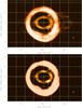 |
Fig. 9 Addition of all position-velocity diagrams obtained along all the axes in the east-west direction. Above we show the result obtained for 12CO J = 3−2 emission, below the result for the 13CO line emission. (The color scale for 13CO is adapted to emphasize the weaker inner ring.) In the right bottom corner of both boxes two little rectangles are plotted to show spatial and spectral resolutions: along the Y-axis the larger rectangle (on the left) shows the beam size (0.17′′), the little rectangle (on the right) the pointing precision (0.01′′); along the X-axis their dimension correspond to the data spectral resolution (0.2 km s-1). See Sect. 6 for more details. |
In Fig. 9 we present the addition of all the position-velocity diagrams obtained along all the east-west axes we can have, that is, the diagrams obtained through all the pixels in the north-south axis. The whole brightness distribution is hence represented here with respect to the RA-offset and LSR-velocity axes. The analysis of this plot best reveals the overall kinematics of the rings, since ring deprojected sizes are shown at maximum RA-offsets, and ring expansion velocities can be deduced from maximum measured LSR-velocities (divided by cos(i)). We note that these composite PV diagrams shown in Fig. 9 were obtained from 0.2 km s-1 resolution maps. For a perfect ring-like distribution in expansion, the brightness represented in Fig. 9 should match an ellipse. We see that this is the case for the inner ring, for which we measure a systemic LSR velocity of 80.65 ± 0.10 km s-1 at a position of 0.03 ± 0.01′′ eastward (the center represented by the intersection of two perpendicular yellow dotted lines). No significant departures from isotropic distribution and radial expansion are found in the inner ring, except for moderate variations in the brighness distribution. The angular resolution is hardly high enough to resolve the inner ring, but the adequate fit with two concentric ellipses (yellow solid lines in Fig. 9) is compatible with a ballistic expansion (i.e., Hubble-type, with radial speed proportional to distance). We obtain at 0.9′′ (the innermost rim) a deprojected expansion velocity of 2.9 km s-1 and 4.2 km s-1 at 1.3′′ (the outermost rim). We note that here we assume that the rings are flat, circularly symmetric, and that their expansion velocity is radial, so that projected speeds are measured at RA−offset = 0′′, and deprojected sizes at maximum RA offsets.
An analysis of the spatio-kinematics of the large ring is complex: ellipses (red solid lines) do not fit any of the rims well, and they are not at all concentric. For the center of the ellipse that best fits the outermost rim, we deduce a systemic LSR velocity of 80.3 ± 0.1 km s-1 (the center being at 0.4′′ eastward); for the innermost rim, a systemic velocity of 79.8 ± 0.1 km s-1 is deduced (the center at 0.2′′ eastward). The systemic LSR velocity of 80.0 km s-1 adopted by Castro-Carrizo et al. (2012) approximately corresponds to the mean of the two measured values for the large ring. The difference of 0.5 km s-1 between the LSR velocities of the two rims is in agreement with the interpretation of a long-duration ejection (of ~40 yr) as described by Castro-Carrizo et al. (2012). (The centroid of the two red ellipses in Fig. 9 is represented by the cross of two perpendicular red dotted lines.) For the large ring we measure a deprojected expansion velocity of 5.5 km s-1 at 2.4′′, and of 8.4 km s-1 at 3.6′′, which supports some type of ballistic expansion that is confirmed by the model fitting in Sect. 7.
The shifts in the position and velocity centroids of both rings we currently deduce are compatible with those found by Castro-Carrizo et al. (2012). As discussed in that paper, the simplest explanation for this remarkable property is to assume that the central star is a binary and that both components were ejected from different positions in the orbit of the primary around the center of gravity. We also confirm that a secondary with a very low mass is required, as low as ~0.2 M⊙ (see details in Castro-Carrizo et al. 2012). The complex structure and dynamics of the large ring are compatible with this interpretation, provided that, as suggested in that paper and described before, its ejection occurred during a relatively long time (around 40 yr, to be compared with an orbital period of 90 yr).
The mean expansion velocity of the large ring is 7.0 km s-1, and 3.6 km s-1 for the small ring. With the current data we deduce a velocity gradient across the inner ring (V/r~ 3.3 km s-1/′′) larger than the gradient in the larger ring (~2.3 km s-1/′′). In other words, if we apply the ballistic law derived for the large ring to the small ring, we would obtain speeds that are a 30% lower than they actually are. This again shows the independent characteristics of the two rings.
In Fig. 10 we show two position-velocity diagrams obtained along the north-south axes that go through the ring centers. These data confirm the different ages for the two rings and are consistent with the values estimated by Castro-Carrizo et al. (2012). Here we deduce an age of 1420 ± 150 yr for the large ring and 900 ± 40 yr for the small ring (for a deduced inclination of 17° for the nebular symmetry axis with respect to the sky plane), which were deduced from the V/r gradients that best fit the current data (red and blue solid lines in Fig. 10) by considering the whole emission obtained for each ring.
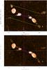 |
Fig. 10 Position-velocity diagrams obtained along two nearby north-south axes for the 12CO J = 3−2 line emission. In the plot above, the axis crossed the center of the innermost ring (0.03′′ eastward), in the one below the center of the outermost ring (i.e., 0.3′′ eastward). In the right bottom corner of both boxes we plot two small rectangles to show the resolutions, similar to those in Fig. 9. Colored solid lines are plotted to show the different position-velocity gradients. More details can be found in Sect. 6. |
An extension toward the center in the northermost part of the inner ring (green arrow in Fig. 10) is detected in these PV diagrams. It corresponds to the departure from symmetry described in point (1) at the beginning of this section, which results in an increase in width of the northern innermost rim of the smaller ring (green arrow in Fig. 4). In the PV diagrams in Fig. 10 this elongation in brightness suggests a flaring of the inner ring toward the crown-like structure detected at ~70 km s-1 and 0.5′′ southward, which is additional evidence that the two structures are related.
It is more difficult to analyze by visual inspection the kinematics and lifetimes of the crown-shaped structures than those of the equatorial rings. While the central rings only present equatorial expansion, the crown-shaped structures have a significant additional axial expansion, as deduced from their high (projected) expansion velocities and in agreement with an overall radial expansion. However, the gradients obtained between the two northern crown components and between the two southern components (yellow dotted line in Fig. 10) are clearly closer to the gradient measured for the inner ring (blue solid line) and very different from the gradient measured for the large ring (red solid line). This is expected if they satisfy the same ballistic law, that is, if they were ejected at the same time. This therefore suggests that the crown-shaped structures and the inner ring were triggered almost simultaneously. Consistently, in the simple model described in Sect. 7, the same ballistic law is applied for the crowns and the inner ring to fit the data. This independent analysis would hence be in agreement with the interpretation made in Sect. 3 that the inner ring and the crowns are all part of the same hourglass-shaped structure.
Finally, in the upper plot of Fig. 10 we also show the (tentatively detected) new component described at the end of Sect. 3 (also marked in Fig. 1).
7. Modeling
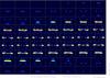 |
Fig. 11 Model predictions to reproduce the 12CO J = 3−2 channel maps presented in Fig. 1 (same contours and color scale). More details can be found in Sect. 7. |
Only 12CO and 13CO J = 3−2 channel maps are currently available, and other information, such as single-dish profiles, are also scarce for M 2–9. Under these conditions, it is not sensible to perform a very detailed modeling. We merely performed a simplified fitting, assuming axial symmetry, simple laws for the physical conditions, and reasonable values for some parameters that are not well constrained by the data. The predictions of our model are shown in Fig. 11 for 12CO J = 3−2 and a general description of the model nebula is provided in Fig. 12, where the distribution of the molecule-rich gas and its main properties are shown for a plane perpedicular to the equator. The structures in the obtained maps are reasonably reproduced by using simple axially symmetric distributions that expand with simple velocity laws, and whose excitation conditions change following simple equations.
Following our direct interpretation of the data, Sects. 3 and 4, we assume three components in our model nebula: an inner equatorial ring, an outer equatorial ring-like component, and two crown-shaped structures parallel to the equatorial plane, but well separated from it (see Fig. 12). For the sake of simplicity, we assume axial symmetry, although, as discussed before, the rings (or torus-like structures) are not exactly axisymmetric. The azimuthal variations of the velocity and density (most likely due to the variable systemic velocity of the star) are very complex second-degree effects, and we neglect them in our modeling. Therefore, the different brightness distributions found for the western and eastern observational features coming from the outer ring cannot be reproduced by our calculations. We only aim at reproducing the average of what we see from both ring parts.
A distance to M 2–9 of 650 pc is adopted in this paper for the same reasons as in Castro-Carrizo et al. (2012), which is also consistent with most of the literature for this source. We note, however, that Corradi et al. (2011) proposed a greater distance of 1300 pc. We also note that our nebula mass estimates depend on (distance)2, densities on (distance)-1, and sizes and lifetimes linearly on distance. Velocities are independent of distance.
The density is assumed to be constant in the inner ring and in the crowns, with values of 5 × 10⁵ and 2 × 104 cm-3, respectively. The density decreases proportionally with the distance to the star in the outer ring, with a central value of 2.5 × 105 cm-3. The same law is assumed for the temperature in our three components, with characteristic values of 70 K, 50 K, and 90 K, respectively. More details can be found in Fig. 12.
The total nebular mass derived from our fitting is ~5.4 × 10⁻³M⊙: a mass of ~5.0 × 10⁻³M⊙ is derived for the outer ring, ~2 × 10⁻⁴M⊙ for the inner ring, and ~10-4M⊙ for the crown-like structures. We note that these values result from the fitting of 12CO and 13CO J = 3−2 channel maps, and although 12CO J = 3−2 emission is optically thick in the rings, this is not the case for the 13CO line emission nor for the 12CO emission in the crown-shaped structures. Furthermore, no significant flux is expected to be filtered out in the current J = 3−2 interferometric data (Sect. 3).
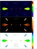 |
Fig. 12 Model used to obtain the predictions of the 12CO J = 3−2 emission presented in Fig. 11, and with which we can also reproduce the data obtained for 13CO. The sketch of the model nebula shows the CO-rich gas distribution in a plane containing the axis of symmetry and perpendicular to the equatorial plane; we recall that axial symmetry is assumed. The axis and the equator correspond in our drawings to the vertical and horizontal axes that intersect at the nebula center, i.e., at the small cross drawn in the center of the panels. The three main components of our model can be identified: the inner equatorial torus (with the highest density), the outer more extended ring, and the crown-shaped structure (with the lowest density and well outside the equatorial plane). At the top, the particle density (cm-3) is represented in color scale. In the middle panel, we show the kinetic temperatures (K); note the relatively high temperatures in the crown. The velocity field is shown at the bottom (km s-1, see the modulus in color scale and some velocity vectors). More details can be found in Sect. 7. |
We find that for all components, purely ballistic expansion velocities (radial velocities with moduli increasing proportionally with the distance to the center within the component) can explain the observed maps per velocity channel. These simple velocity fields are often found in PPNe and young PNe. The velocity field is also depicted in Fig. 12. Following our previous discussion (Sect. 6), the centroid of the LSR velocity of the large ring is assumed to be shifted by –0.7 km s-1 with respect to that of the other two components, inner ring, and crown-shaped structures (this effect is not represented in the figure, where only the expansion velocity vectors are shown).
We assume local thermodynamic equilibrium (LTE) populations for the relevant rotational levels. This is reasonable for these low-J CO transitions in the dense material expected in our nebula, n≳ 105 cm, since their Einstein coefficients are at least ten times smaller than the typical collisional rates; see further discussion in Bujarrabal et al. (2013, 2017). Nevertheless, we must keep in mind that the rotational temperatures we use in our calculations may just represent J-averaged excitation temperatures and not true kinetic temperatures. Since high-J levels can obviously be less populated in reality than for LTE, these rotational temperatures are probably a lower limit to the actual temperatures in the less dense gas. On the other hand, the use of LTE significantly simplifies the calculations and provides an easier interpretation of the possible uncertainties in the fitting. We will study the CO level population in a forthcoming paper in more detail by including the analysis of CO J = 6−5 data.
Because we assumed thermalized level populations, it is not possible to distinguish the effects of the density and relative CO abundances, X(12CO, 13CO). Fortunately, X seems relatively well constrained in the best-studied objects, particularly X(13CO), which is the basic parameter to determine the total density and mass because of the lower opacity of the 13CO lines. Our previous works always yielded X(13CO) ranging between 1 and 2 × 10⁻⁵ in PPNe and young PNe. We here adopt X(13CO) ~1.5 × 10⁻⁵. In order to match the relative low 12CO/13CO intensity ratio, we need a relatively low abundance ratio, we adopt X(12CO) ~1.5 × 10⁻⁴; similarly low ratios are often found in similar objects. 13CO J = 3−2 is weaker than 12CO J = 3−2, but by just a factor ~2–3 (Sect. 4), at least in the equatorial rings, which implies that the 12CO line is moderately opaque in these components. Under these conditions, their typical temperatures can be easily deduced from the obtained peak brightness (in K units), as confirmed by our calculations. However, the fact that the 13CO J = 3−2 peak brightness is significantly lower confirms that this line remains optically thin.
8. Relation between equatorial rings and axial lobes
With the data analyzed by Castro-Carrizo et al. (2012), it was proposed that the two rings detected in CO emission and the two axial lobes seen in the optical image by Balick et al. (1997) are directly related. We note that while the analysis of low-J CO emission allows us to trace the bulk of the cold matter in the nebula, in visible light we can only see those parts of the nebula that are illuminated by the star, or are ionized either by stellar photons or by shocks with other winds. All in all, the parts seen in the optical should not represent a large portion of the mass (Castro-Carrizo et al. 2001). The new data presented here provide additional information to understand the nebula shaping, by considering the complementary pictures obtained in the visible and in molecular emission.
By comparing the optical and radio-wavelength brightness distributions (Figs. 2 and 3), we have deduced that the crown-shaped structures and the inner ring detected in CO emission are the molecular counterparts of the inner hourglass structure (as defined in Fig. 3) detected in optical light. We do not have clear clues as to why CO emission is only detected in these small fractions (crown-shaped and ring) of the inner hourglass structure. A higher signal-to-noise ratio may be needed to detect the whole hourglass, or otherwise CO may be photodissociated elsewhere. We note that Castro-Carrizo et al. (2001) deduced a photodissocation region ten times more massive than the molecular and the ionized gas components. In any case, from the analysis made in Sect. 6, it seems clear that the crowns and the inner ring were triggered simultaneously ~900 yr ago, and that they are hence part of the same ejection event.
From the optical image we can deduce a close relation between the small hourglass (detected in CO) and the large inner optical lobes (as defined in Fig. 3). The confirmation in Sect. 3 that no significant flux is filtered out implies that no other large amounts of CO are expected in other parts of the nebula. Recent estimates of the kinematical age of the inner optical lobes by Clyne et al. (2015) agree with the estimate derived by us for the inner hourglass, which validates the proposition that both components were triggered by the same ejection and are hence part of the same outflow.
On the other side, no new clear hints were found that might help to understand the relation between the large older ring and the optical nebula. No similar hourglass-type counterpart is detected coincident with the large optical lobes. Nevertheless, the good spatial fitting between the large molecular ring and the outer optical lobes, and the well-resolved flaring structure observed in the eastern part of the ring strongly suggest that both are complementary parts of the same structure, triggered by a first outflow ~1400 yr ago. The agreement with the kinematical age derived by Clyne et al. (2015) also seems to confirm such scenario.
9. Conclusions
Channel maps of 12CO and 13CO J = 3−2 line emission were presented for the first time here, with an angular resolution of ~0.18′′ on average.
We find the two ring-like structures that have been observed in 12CO J = 2−1 emission by Castro-Carrizo et al. (2012). Their distribution and kinematics were analyzed with an improved signal-to-noise ratio and angular resolution of the new data, which allowed us to validate the main findings derived from the J = 2−1 transition.
In addition, two crown-shaped structures parallel to (above and below) the equatorial plane were detected to coincide with a small hourglass seen in the visible, located close to the equator in between the inner and outer optical lobes. The molecular inner ring would also be part of this hourglass.
Two separate axial ejections seem to have created the structures seen in visible light and the molecular gas distribution in M 2–9. The first would have occurred ~1400 yr ago to form the outer optical lobes and the large equatorial molecular ring. A second ejection would have formed the inner hourglass seen in CO and in the optical about 900 yr ago. The kinematical times estimated by Clyne et al. (2015) would indicate that this inner hourglass (crowns and inner ring) and the inner optical lobes (as defined in Fig. 3) were triggered simultaneously. All in all, it is worth noting that according to Castro-Carrizo et al. (2001), most of the nebular material would be neutral atoms, which are not included in this description.
The main component detected in continuum emission is very compact and unresolved with an angular resolution of 0.17′′. However, continuum emission is also tentatively detected along the inner equatorial ring (from 0.8−1.4′′ in radius).
Predictions for both 12CO and 13CO J = 3−2 channel maps have been obtained with a radiative-transfer model to build a simplified picture of the spatio-dynamical distribution in M 2–9. The complementary information provided by the emission from the two isotopes constrains the total mass of the nebula to 5 × 10⁻³M⊙, ~90% of which is in the large molecular ring. As usual in proto-PNe, the velocity field is found to follow a ballisticlaw for all components, and the law associated with the larger outflow (i.e., its kinematical age) is different from that of the small hourglass. Densities and temperatures follow simple laws decreasing with radius.
Finally, we note that the current data confirm the results obtained by Castro-Carrizo et al. (2012), in particular that the characteristics of the two rings can be explained by two ejections from a binary stellar system with a very low-mass secondary. Additional data would be needed to delve deeper into the details of the proposed scenario.
Available in http://www.apex-telescope.org/observing/archiving/
Acknowledgments
This paper makes use of the following ALMA data: ADS/JAO.ALMA#2013.0.00458.S. ALMA is a partnership of ESO (representing its member states), NSF (USA) and NINS (Japan), together with NRC (Canada), NSC and ASIAA (Taiwan), and KASI (Republic of Korea), in cooperation with the Republic of Chile. The Joint ALMA Observatory is operated by ESO, AUI/NRAO and NAOJ. The data presented here were first reduced by CASA (ALMA default calibration software), but a second iteration in the data reduction and later analysis for presentation was made by using the MAPPING package available in the GILDAS software (http://www.iram.fr/IRAMFR/GILDAS). Also, Fig. 5 was obtained from few 30 m-IRAM telescope acquisitions and data from the APEX telescope data archive. IRAM is supported by INSU/CNRS (France), MPG (Germany) and IGN (Spain). APEX is a collaboration between the Max-Planck-Institut fur Radioastronomie, the European Southern Observatory, and the Onsala Space Observatory. This work has also been supported by the Spanish MINECO, grants AYA2016-78994-P and FIS2012-32096, and by the European Research Council (ERC) Grant 610256: NANOCOSMOS.
References
- Balick, B., & Frank, A. 2002, ARA&A, 40, 439 [NASA ADS] [CrossRef] [Google Scholar]
- Balick, B., Icke, V., Mellema, G., & NASA 1997, in NASA Press Release, ed. NASA, GRIN DataBase Number: GPN–2000–000953 [Google Scholar]
- Bujarrabal, V., Castro-Carrizo, A., Alcolea, J., et al. 2013, A&A, 557, L11 [NASA ADS] [CrossRef] [EDP Sciences] [Google Scholar]
- Bujarrabal, V., Castro-Carrizo, A., Alcolea, J., et al. 2017, A&A, 597, L5 [NASA ADS] [CrossRef] [EDP Sciences] [Google Scholar]
- Castro-Carrizo, A., Bujarrabal, V., Fong, D., et al. 2001, A&A, 367, 674 [NASA ADS] [CrossRef] [EDP Sciences] [Google Scholar]
- Castro-Carrizo, A., Neri, R., Bujarrabal, V., et al. 2012, A&A, 545, A1 [NASA ADS] [CrossRef] [EDP Sciences] [Google Scholar]
- Clyne, N., Akras, S., Steffen, W., et al. 2015, A&A, 582, A60 [NASA ADS] [CrossRef] [EDP Sciences] [Google Scholar]
- Corradi, R. L. M., Balick, B., & Santander-García, M. 2011, A&A, 529, A43 [NASA ADS] [CrossRef] [EDP Sciences] [Google Scholar]
- De Marco, O. 2009, PASP, 121, 316 [NASA ADS] [CrossRef] [Google Scholar]
- Di Francesco, J., Johnstone, D., Kirk, H., MacKenzie, T., & Ledwosinska, E. 2008, ApJS, 175, 277 [NASA ADS] [CrossRef] [Google Scholar]
- Doyle, S., Balick, B., Corradi, R. L. M., & Schwarz, H. E. 2000, AJ, 119, 1339 [NASA ADS] [CrossRef] [Google Scholar]
- Frank, A., & Blackman, E. G. 2004, ApJ, 614, 737 [NASA ADS] [CrossRef] [Google Scholar]
- Hrivnak, B. J., Lu, W., Bohlender, D., et al. 2011, ApJ, 734, 25 [NASA ADS] [CrossRef] [Google Scholar]
- Hubble Legacy Archive 2013, NASA, ESA – Processing: Judy Schmidt, Astronomical Picture of the Day [Google Scholar]
- Livio, M., & Soker, N. 2001, ApJ, 552, 685 [NASA ADS] [CrossRef] [Google Scholar]
- Lykou, F., Chesneau, O., Zijlstra, A. A., et al. 2011, A&A, 527, A105 [NASA ADS] [CrossRef] [EDP Sciences] [Google Scholar]
- Reid, M. J., Schneps, M. H., Moran, J. M., et al. 1988, ApJ, 330, 809 [NASA ADS] [CrossRef] [Google Scholar]
- Sahai, R., Morris, M., Sánchez Contreras, C., & Claussen, M. 2007, AJ, 134, 2200 [NASA ADS] [CrossRef] [Google Scholar]
- Sánchez Contreras, C., Alcolea, J., Bujarrabal, V., & Neri, R. 1998, A&A, 337, 233 [NASA ADS] [Google Scholar]
- Schmeja, S., & Kimeswenger, S. 2001, A&A, 377, L18 [NASA ADS] [CrossRef] [EDP Sciences] [Google Scholar]
- Schwarz, H. E., Aspin, C., Corradi, R. L. M., & Reipurth, B. 1997, A&A, 319, 267 [NASA ADS] [Google Scholar]
- Smith, N., & Gehrz, R. D. 2005, AJ, 129, 969 [NASA ADS] [CrossRef] [Google Scholar]
- Soker, N. 2001, ApJ, 558, 157 [NASA ADS] [CrossRef] [Google Scholar]
- Zweigle, J., Neri, R., Bachiller, R., Bujarrabal, V., & Grewing, M. 1997, A&A, 324, 624 [NASA ADS] [Google Scholar]
All Figures
|
Fig. 1 Channel maps of the 12CO J = 3−2 line emission toward M 2–9. The center is given by the position of compact continuum emission, here subtracted, at J2000 coordinates RA = 17:05:37.966, Dec = −10:08:32.63. The LSR velocities are specified in the top left corner of each panel. Contours are shown from 4 ×σ with a spacing of 15 ×σ (where the root-mean-square noise is 2 mJy beam-1, which corresponds to 0.66 K in Rayleigh-Jeans-equivalent TMB units) as a white solid line, and at −4 ×σ as dashed red lines. The synthesized beam is 0.̋19 × 0.̋16 with the major axis PA = 116°, and is drawn in the bottom right corner of the last panel. More details can be found in Sect. 3. |
| In the text | |
|
Fig. 2 In contours, one over three 12CO J = 3−2 channel maps are presented with 8 km s-1 channel spacing, overlaid on the HST [NII] image published by Clyne et al. (2015) in color scale. As in Fig. 1, we detect some emission in between that from the inner ring and the crown-shaped structures. Contours are shown from 4 ×σ with a spacing of 15 ×σ (for σ = 1.5 mJy beam-1 = 0.32 K) as a solid line, and at −4 ×σ as dashed gray lines. The synthesized beam is 0.̋26 × 0.̋19 in size with the major axis PA = −18°. |
| In the text | |
|
Fig. 3 Left: velocity-integrated 12CO J = 2−1 line emission in color scale (blue scale for the 68–80.3 km s-1 spectral range and orange for the 80.3–94 km s-1 interval) superimposed on the optical image obtained with the Hubble Space Telescope (Hubble Legacy Archive 2013). More details can be found in Sect. 3 and Fig. 1. Right: brightness 12CO J = 3−2 emission at the central velocity (LSR velocity 80.4 km s-1, after integrating in 0.4 km s-1) in contours overlaid on the optical image in color scale. Contours are plotted at 4 ×σ, and from 10 ×σ every 10 ×σ. The synthesized beam is shown in the right bottom corner of both plots. Labels are given to each of the main components identified in the optical image, which are discussed in Sect. 8. |
| In the text | |
|
Fig. 4 Velocity-integrated 12CO J = 3−2 line emission, similar to that shown in Fig. 3 left. At the center, the continuum peak emission is represented by a red contour, which probably traces the position of the stellar system (see Sect. 5). Above, the data are presented in a box of 8.8′′× 4.8′′ in size, and 4.0′′× 2.2′′ in the plot below. Ellipses are plotted to help visualize the departures from symmetry, and the synthesized beam is shown in the right bottom corner of both plots. More details in Sects. 3 and 6. |
| In the text | |
|
Fig. 5 Total integrated 12CO J = 3−2 emission compared with single-dish line profiles obtained with the 30 m IRAM and the APEX telescopes (see Sect. 3). |
| In the text | |
|
Fig. 6 Channel maps of the 13CO J = 3−2 line emission toward M 2–9. The center is given by the position of the compact continuum emission, here subtracted, at J2000 coordinates RA = 17:05:37.966, Dec = −10:08:32.63. The LSR velocities are specified in the top left corner of each panel. Contours are shown in 4 ×σ with a spacing of 7 ×σ (where the root-mean-square noise is 2.5 mJy beam-1, which corresponds to 0.82 K in Rayleigh-Jeans-equivalent TMB units) as a white solid line, and at −4 ×σ as dashed red lines. The synthesized beam is 0.̋20 × 0.̋17 with the major axis PA = −79° and is drawn in the bottom right corner of the last panel. |
| In the text | |
|
Fig. 7 Total integrated 12CO and 13CO J = 3−2 emission in M 2–9 is shown in black, the emission integrated over the smaller ring is presented in red. Vertical red dotted lines are plotted at LSR velocities 80.65 (inner ring Vsys), 77.65, and 83.65 km s-1, and blue dotted lines at 80 (outer ring Vsys), 74, and 86 km s-1. |
| In the text | |
|
Fig. 8 Continuum emission in contours overlaid on the optical HST image (Hubble Legacy Archive 2013) in M 2–9. Contours are shown at 4, 8, and 12σ and from then on with a spacing of 12σ (where the root-mean-square noise is 0.1 mJy beam-1) as a solid line and at −4σ as a dashed line. The synthesized beam is 0.̋27 × 0.̋23 with the major axis PA = 122° and is drawn in the bottom right corner of the last panel. The ellipses delimiting the rims of the inner ring in Fig. 3 are also plotted here, centered at [+0.̋03, −0.̋03] according to the analysis in Sect. 6. |
| In the text | |
|
Fig. 9 Addition of all position-velocity diagrams obtained along all the axes in the east-west direction. Above we show the result obtained for 12CO J = 3−2 emission, below the result for the 13CO line emission. (The color scale for 13CO is adapted to emphasize the weaker inner ring.) In the right bottom corner of both boxes two little rectangles are plotted to show spatial and spectral resolutions: along the Y-axis the larger rectangle (on the left) shows the beam size (0.17′′), the little rectangle (on the right) the pointing precision (0.01′′); along the X-axis their dimension correspond to the data spectral resolution (0.2 km s-1). See Sect. 6 for more details. |
| In the text | |
|
Fig. 10 Position-velocity diagrams obtained along two nearby north-south axes for the 12CO J = 3−2 line emission. In the plot above, the axis crossed the center of the innermost ring (0.03′′ eastward), in the one below the center of the outermost ring (i.e., 0.3′′ eastward). In the right bottom corner of both boxes we plot two small rectangles to show the resolutions, similar to those in Fig. 9. Colored solid lines are plotted to show the different position-velocity gradients. More details can be found in Sect. 6. |
| In the text | |
|
Fig. 11 Model predictions to reproduce the 12CO J = 3−2 channel maps presented in Fig. 1 (same contours and color scale). More details can be found in Sect. 7. |
| In the text | |
|
Fig. 12 Model used to obtain the predictions of the 12CO J = 3−2 emission presented in Fig. 11, and with which we can also reproduce the data obtained for 13CO. The sketch of the model nebula shows the CO-rich gas distribution in a plane containing the axis of symmetry and perpendicular to the equatorial plane; we recall that axial symmetry is assumed. The axis and the equator correspond in our drawings to the vertical and horizontal axes that intersect at the nebula center, i.e., at the small cross drawn in the center of the panels. The three main components of our model can be identified: the inner equatorial torus (with the highest density), the outer more extended ring, and the crown-shaped structure (with the lowest density and well outside the equatorial plane). At the top, the particle density (cm-3) is represented in color scale. In the middle panel, we show the kinetic temperatures (K); note the relatively high temperatures in the crown. The velocity field is shown at the bottom (km s-1, see the modulus in color scale and some velocity vectors). More details can be found in Sect. 7. |
| In the text | |
Current usage metrics show cumulative count of Article Views (full-text article views including HTML views, PDF and ePub downloads, according to the available data) and Abstracts Views on Vision4Press platform.
Data correspond to usage on the plateform after 2015. The current usage metrics is available 48-96 hours after online publication and is updated daily on week days.
Initial download of the metrics may take a while.