| Issue |
A&A
Volume 600, April 2017
|
|
|---|---|---|
| Article Number | A61 | |
| Number of page(s) | 18 | |
| Section | Interstellar and circumstellar matter | |
| DOI | https://doi.org/10.1051/0004-6361/201628463 | |
| Published online | 30 March 2017 | |
Deuteration of ammonia in the starless core Ophiuchus/H-MM1⋆
1 Max-Planck-Institute for Extraterrestrial Physics (MPE), Giessenbachstr. 1, 85748 Garching, Germany
e-mail: This email address is being protected from spambots. You need JavaScript enabled to view it.
2 Department of Physics, PO Box 64, University of Helsinki, 00014 Helsinki, Finland
3 Université Grenoble Alpes, IPAG, 38000 Grenoble, France
4 CNRS, IPAG, 38000 Grenoble, France
5 Dunlap Institute for Astronomy and Astrophysics, University of Toronto, 50 St. George Street, Toronto M5S 3H4, Ontario, Canada
6 Max-Planck-Institut für Radioastronomie, Auf dem Hügel 69, 53121 Bonn, Germany
7 Harvard-Smithsonian Center for Astrophysics, 60 Garden Street, Cambridge MA 02138, USA
8 Department of Physics, 4-181 CCIS, University of Alberta, Edmonton, AB T6G 2E1, Canada
9 I. Physikalisches Institut, Universität zu Köln, Zülpicher Strasse 77, 50937 Köln, Germany
10 Steward Observatory, University of Arizona, 933 North Cherry Avenue, Tucson, AZ 85721, USA
Received: 9 March 2016
Accepted: 16 December 2016
Abstract
Context. Ammonia and its deuterated isotopologues probe physical conditions in dense molecular cloud cores. The time-dependence of deuterium fractionation and the relative abundances of different nuclear spin modifications are supposed to provide a means of determining the evolutionary stages of these objects.
Aims. We aim to test the current understanding of spin-state chemistry of deuterated species by determining the abundances and spin ratios of NH2D, NHD2 and ND3 in a quiescent, dense cloud.
Methods. Spectral lines of NH3, NH2D, NHD2, ND3 and N2D+ were observed towards a dense, starless core in Ophiuchus with the APEX, GBT and IRAM 30-m telescopes. The observations were interpreted using a gas-grain chemistry model combined with radiative transfer calculations. The chemistry model distinguishes between the different nuclear spin states of light hydrogen molecules, ammonia and their deuterated forms. Different desorption schemes can be considered.
Results. High deuterium fractionation ratios with NH2D/NH3 ~ 0.4, NHD2/ NH2D ~ 0.2 and ND3/ NHD2 ~ 0.06 are found in the core. The observed ortho/para ratios of NH2D and NHD2 are close to the corresponding nuclear spin statistical weights. The chemistry model can approximately reproduce the observed abundances, but consistently predicts too low ortho/para-NH2D, and too large ortho/para-NHD2 ratios. The longevity of N2H+ and NH3 in dense gas, which is prerequisite to their strong deuteration, can be attributed to the chemical inertia of N2 on grain surfaces.
Conclusions. The discrepancies between the chemistry model and the observations are likely to be caused by the fact that the model assumes complete scrambling in principal gas-phase deuteration reactions of ammonia, which means that all the nuclei are mixed in reactive collisions. If, instead, these reactions occur through proton hop/hydrogen abstraction processes, statistical spin ratios are to be expected. The present results suggest that while the deuteration of ammonia changes with physical conditions and time, the nuclear spin ratios of ammonia isotopologues do not probe the evolutionary stage of a cloud.
Key words: astrochemistry / ISM: molecules / ISM: abundances / ISM: clouds
Based on observations carried out with The Atacama Pathfinder Experiment (APEX), the Robert C. Byrd Green Bank Telescope (GBT), and the IRAM 30 m Telescope. APEX is a collaboration between Max-Planck Institut für Radioastronomie (MPIfR), Onsala Space Observatory (OSO), and the European Southern Observatory (ESO). GBT is managed by the National Radio Astronomy Observatory, which is a facility of the National Science Foundation operated under cooperative agreement by Associated Universities, Inc. IRAM is supported by INSU/CNRS (France), MPG (Germany), and IGN (Spain).
© ESO, 2017
1. Introduction
Ammonia belongs to the most useful probes of the dense cores of molecular clouds owing to its energy spectrum and chemical properties (Ho & Townes 1983; Benson & Myers 1989; Tafalla et al. 2002; Friesen et al. 2009). The molecule can survive in the gas phase also in the cold, dense interior parts of starless and pre-stellar cores, and in these regions, reactions with deuterated ions convert part of NH3 to NH2D, NHD2 and ND3 (Rodgers & Charnley 2001). Ammonia and its deuterated isotopologues are also formed on grain surfaces through H/D-atom addition reactions to N atoms (Brown & Millar 1989; Fedoseev et al. 2015). Substantial deuteration in both phases occurs after the disappearance of CO from the gas phase, and needs some time to take effect, so the relative abundances of the mentioned molecules can give an idea of the evolutionary stage of a dense core (Roueff et al. 2005; Flower et al. 2006a; Roueff et al. 2015). The N2D+/ N2H+ abundance ratio has already been used extensively for this purpose (Crapsi et al. 2005; Pagani et al. 2009b).
Besides enabling nuanced investigation into deuteration, spectral line observations of NH3, NH2D, NHD2 and ND3 test our understanding of spin-state chemistry, that is, selection rules in chemical reactions that determine the relative abundances of different nuclear spin symmetry species or “modifications”. Each spectral line observed from these molecules belongs to one of the two spin modifications of NH3, NH2D or NHD2, or one of the three spin modifications of ND3. The abundance ratios of these modifications, which must be treated as separate chemical species, can deviate from their nuclear spin statistical ratios and are predicted to change with time (Faure et al. 2013; Sipilä et al. 2015a,b).
The spin symmetry species of a molecule is defined based on how the nuclear spin wave function transforms under symmetry operations such as the interchange or the permutation of identical nuclei. For molecules containing only H nuclei, there is a one to one correspondence between the symmetry and the nuclear spin angular momentum, but this is not true for molecules with multiple D nuclei (Hugo et al. 2009). Schmiedt et al. (2016) have recently shown that the spin angular momentum and the permutation symmetry are, after all, inherently coupled, and that it is possible to construct an unequivocal and practical representation for each spin angular momentum – symmetry species using the Young diagrams. In the present study, chemical species are distinguished solely by their nuclear spin symmetries.
The statistical weight of a symmetry species is the number of possible nuclear spin functions that have that symmetry. When there are no more than three spin modifications, it is customary to call the species with the largest nuclear spin statistical weight “ortho”, and the one with the lowest weight “para”. If there is a third one, this is called “meta”. For example, the three elementary spin functions of the deuteron, | 1,1 ⟩, | 1,0 ⟩ and | 1,−1 ⟩, can combine in ND3 in 27 different ways, and these combinations can be arranged into a set of 27 orthogonal functions, which form an irreducible representation of the appropriate permutation group S3. Of these functions, 10 have symmetry A1 (“meta”), 1 has symmetry A2 (“para”), and 16 have symmetry E (“ortho”) in S3 (Bunker & Jensen 2006; Sipilä et al. 2015b; Daniel et al. 2016b, see their Appendix A).
The abundances of all three deuterated forms of ammonia have been previously estimated in the protostellar core “B1-b” of Barnard 1 in Perseus (Lis et al. 2002b, 2006; Roueff et al. 2005), and in the starless core (“I16293E”) of the dark cloud L1689N in Ophiuchus (Roueff et al. 2005; Gerin et al. 2006). The fractionation ratios are similar in these two objects. The recent analysis of these observations by Daniel et al. (2016b) gives [ NH2D ] / [ NH3 ] ≳ [ NHD2 ] / [ NH2D ] ≈ 0.2, [ ND3 ] / [ NHD2 ] ≈ 0.05−0.10. In both cores, the ortho/para ratios of NH2D and NHD2 were found to be close to their statistical values, 3:1 and 2:1, respectively. The interpretation of chemical data from these two, bright sources of deuterated ammonia is complicated by the possibility of enhanced evaporation from grains due to shocks. The Barnard 1 core contains two, albeit very young and low-mass protostars driving outflows (B1-bS and B1-bN; Hatchell et al. 2007; Hirano & Liu 2014; Gerin et al. 2015). The core in L1689N may be compressed by an outflow from the adjacent protostellar source IRAS 16293-2422 (Lis et al. 2002a; Stark et al. 2004; Gerin et al. 2006).
In the present work, we use the 100-m Robert C. Byrd Green Bank telescope, the 12-m APEX and the IRAM 30-m telescope to determine the abundances of para-NH3, meta-ND3 and both ortho and para modifications of NH2D and NHD2 in the starless core H-MM1 in Ophiuchus (Johnstone et al. 2004; Parise et al. 2011). Through these observations, we obtain a homogenous data set pertaining to a quiescent region, presumably characterised by a simple physical structure, where comparison with chemistry models is more straightforward than in a star-forming core. The observations are interpreted by modelling the chemical evolution of a hydrostatic core resembling H-MM1, and simulating observations towards this model core. Besides the previously published collisional coefficients of NH2D with para-H2 (Daniel et al. 2014), we use newly calculated coefficients for NHD2 and ND3 (Daniel et al. 2016b), in conjunction with the radiative transfer program of Juvela (1997).
The paper is organised as follows. In Sect. 2, we describe the target core and give details of the observations. The direct observational results are presented in Sect. 3. In Sect. 4, we construct a physical model of the core and describe the modelling tools, the collisional coefficients and the chemistry model used in this work. In Sect. 5, we make predictions for the NH3, NH2D, NHD2 and ND3 abundances and the observable line emission from the model core. In Sect. 6, we compare the outcome of the modelling with the observations and discuss the implications of this comparison. Finally, in Sect. 7, we draw our conclusions.
2. Observations
2.1. The target: H-MM1
The dense core H-MM1 in Ophiuchus was discovered by Johnstone et al. (2004) using the Submillimeter Common-User Bolometric Array (SCUBA) on the James Clerk Maxwell Telescope (JCMT). The core was also covered by the JCMT Gould Belt Survey with SCUBA-2 at 450 and 850 μm (Pattle et al. 2015). H-MM1 lies in relative isolation in the eastern part of Lynds 1688, far from sites of active star formation. Parise et al. (2011) detected extended para-D2H+ emission towards this core. Based on the analysis of the para-D2H+ and ortho-H2D+ lines towards its centre, Parise et al. suggested that the average density of the core is high compared to typical starless cores, a few times 105 cm-3. In accordance with the high abundances of the deuterated ions, the deuterium fraction in N2H+ is also extremely high: N2D+/ N2H+ = 0.43 ± 0.11 (Punanova et al. 2016).
In Fig. 1, we show the dust colour temperature (TC) and the H2 column density (N(H2)) maps of the core derived from far-infrared images observed by Herschel (Pilbratt et al. 2010). Contours of the 850 μm emission map from the SCUBA-2 survey of Pattle et al. (2015) are superposed on the N(H2) map.
The Herschel/SPIRE images were extracted from the pipeline-reduced images of the Ophiuchus complex made in the course of the Herschel Gould Belt Survey (André et al. 2010). The data are downloaded from the Herschel Science Archive (HSA)1. We calculated the TC and N(H2) distributions using only the three SPIRE (Griffin et al. 2010) bands at 250 μm, 350 μm and 500 μm, for which the pipeline reduction includes zero-level corrections based on comparison with the Planck satellite data. A modified blackbody function with the dust emissivity spectra index β = 2 was fitted to each pixel after smoothing the 250 μm and 350 μm images to the resolution of the 500 μm image (~ 40″), and resampling all images to the same grid. For the dust emissivity coefficient per unit mass of gas, we adopted the value from Hildebrand (1983), κ250 μm = 0.1 cm2 g-1 (1 /C250 in Table 1 in their paper). Suutarinen et al. (2013) derived a similar value for κ250 μm in the starless core CrA C. According to the derived maps, the dust colour temperature minimum and the column density maximum of the core is found at RA  , Dec. −24°33′33″ (J2000). The line observations presented here were done towards this position. The obtained minimum colour temperature is 12.4 K and the maximum column density is N(H2) = 5.7 × 1022 cm-2. These values are averages over the 40″ beam. The fitted TC overestimates the mass-averaged dust temperature because of line-of-sight temperature variations. This effect is more marked towards the centre of a starless core than on the outskirts of the core (Nielbock et al. 2012; Suutarinen et al. 2013).
Our position lies approximately 13″ northeast from the centre position used by Parise et al. (2011), and approximately 7″ east of the 450 and 850 μm peaks observed with SCUBA-2. In a later section we use the SCUBA-2 maps to derive a simple spherically symmetric model of the core for the purpose of radiative transfer modelling.
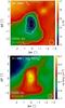 |
Fig. 1 Dust colour temperature (TC, top) and the H2 column density (N(H2), bottom) maps of H-MM1 as derived from Herschel/SPIRE maps at 250, 350, and 500 μm. The distribution of the 850 μm emission observed with SCUBA-2 is indicated with black contours on the N(H2) map. The contour levels are 10 to 50 by 10 MJy sr-1. The column density maximum is marked with a plus sign. The present observations were pointed towards this position, with coordinates RA |
Observed transitions.
2.2. GBT observations
The observations were carried out using the 7-beam K-Band Focal Plane Array (KFPA) at the GBT, with the Versatile GBT Astronomical Spectrometer (VEGAS) backend, as part of the Gould Belt Ammonia Survey (GBT15A-430, PIs: Friesen & Pineda). VEGAS was configured in Mode 20, which uses 8 separate spectral windows per KFPA beam, each with a bandwidth of 23.44 MHz and 4096 spectral channels. The spectral resolution is 5.7 kHz, corresponding to ~ 0.07 km s-1. Observations were performed using in-band frequency switching with a frequency throw of 4.11 MHz. Here we use the NH3(1,1) and (2,2) line maps of a 6′ × 6′ region centered on the column density peak of H-MM1. The integrated NH3(1,1) intensity map of this region is shown in Fig. 2.
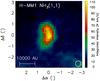 |
Fig. 2 Integrated NH3(1,1) intensity (TMB) map of H-MM1 observed with the GBT. The intensity unit is K km s-1, and the colour scale is given on the right. The 32″ beam size of the GBT at 23.7 GHz is indicated in the bottom right. The APEX and IRAM spectra were taken towards the position indicated with a plus sign. |
These observations were part of a much larger area map of the entire L1688 region during the 15A semester, which will be presented by Friesen & Pineda et al. (in prep.), and carried out on 10′ × 10′ boxes scanned in right ascension with rows separated by 13″ in declination. The scanning rate was 6.2″ s-1, with a data dump every 1.044 s. A fast frequency switching rate of 0.348 s was used, which results in a root mean square noise (RMS) of 0.1 K (on the TMB scale).
The data are calibrated using the GBT KFPA data reduction pipeline (Masters et al. 2011). The data were calibrated to the TMB scale using the gain factors for each beam calibration derived from the Moon observations. The final cubes are created by a custom-made gridder using a tapered Bessel function for the convolution following Mangum et al. (2007)2.
The observed ammonia transitions are indicated in the energy level diagram shown in Fig. 3.
2.3. APEX observations
The centre position of H-MM1 was observed using the upgraded version of the First Light APEX Submillimeter Heterodyne instrument (FLASH; Heyminck et al. 2006) on APEX (Güsten et al. 2006). This instrument, FLASH+ (Klein et al. 2014), operates in the 345 GHz and the 460 GHz atmospheric windows simultaneously, and can record two 4-GHz-wide sidebands separated by 12 GHz in both windows, that is, altogether 4 × 4 GHz frequency bands. The receivers were connected to MPIfR Fast Fourier Transform Spectrometers (XFTTS, Klein et al. 2012) with spectral resolutions of ~ 0.03 and ~ 0.05 km s-1 at 345 and 460 GHz, respectively.
The sky subtraction was done by position switching, using an absolute reference position (RA 16h28m32s, Dec. −24°31′00″, J2000) which, judging from Herschel far-infrared maps is void of dense gas. In the lower frequency window we used two frequency settings, which covered 1) the ground-state lines of para- and meta-ND3 (hereafter pND3 and mND3) at 306.7 and 309.9 GHz, and 2) the ground-state lines of ortho- and para-NH2D (oNH2D and pNH2D) at 332.8 GHz, and the ground-state lines of ortho- and para-NHD2 (oNHD2 and pNHD2) at 335.5 GHz. The first tuning also covered the N2D+(4−3) line at 308.4 GHz. The observations in the 460 GHz window were aimed at the N2D+(6−5) and N2H+(5−4) lines. Because these two lines could be measured simultaneously, the tuning of the 460 GHz receiver was kept constant during the whole observing run.
A list of transitions covered is given in Table 1, mentioning only the most significant to the present study. Here we give the centre frequencies of transitions, upper state energies and Einstein coefficients for spontaneous emission. These parameters are obtained from the Cologne Database for Molecular Spectroscopy, CDMS3. The observed transitions of NH3, NH2D, NHD2 and ND3 are indicated in the energy level diagrams in Figs. 3.
The APEX beamsize (Full width at half maximum, FWHM) is ~ 20″ at 310−330 GHz, and ~ 14″ at 465 GHz. The main beam efficiency, ηMB, is 0.73 at 310−330 GHz, and 0.6 at 465 GHz (Güsten et al. 2006). The observations were carried out between the 29th and 31st May, 2015. The total observing time was 11.4 h. The weather conditions were stable and fairly good (PWV 0.7−1.2 mm). The absolute calibration, pointing and focus were checked by observing Saturn. The system temperatures were in the following ranges: 180−190 K (310 GHz), 230−250 K (335 GHz) and 570−600 K (465 GHz). The resulting RMS noise levels at the mentioned frequencies at a velocity resolution of 0.1 km s-1 were 18, 27 and 33 mK, respectively, on the TMB scale.
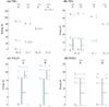 |
Fig. 3 Energies of the lowest rotational levels of NH3a); ND3b); NH2Dc) and NHD2d). The nuclear spin symmetries and their “para”, “meta” and “ortho” appellations are indicated. The ground-state rotation-inversion transition |

2.4. IRAM observations
The column density peak of H-MM1 was observed with the IRAM 30-m telescope on the 5th July, 2015, in acceptable weather conditions (PWV 8−10 mm). Pointing and focus were checked towards QSO 1253-055. The following transitions were observed: oNH2D(111−101) at 85.9 GHz, pNH2D(111−101) at 110.2 GHz and N2D+(2−1) at 154.2 GHz. The measurements were obtained with the EMIR 090 and 150 receivers4 and the VESPA auto-correlator with a spectral resolution of 20 kHz; the corresponding velocity resolutions were 0.04−0.07 km s-1. The beam sizes were 29″, 23″ and 16″ for oNH2D(111−101), pNH2D(111−101) and N2H+(2−1), respectively. The system temperatures ranged from 166 to 310 K depending on the frequency (see Table 2 for the details). The spectra were taken in the position switching mode, using an off position 400′′ East of the target. The integration time for each line was between 15 and 22 min, which resulted in RMS noise levels of 0.08−0.14 K on the TMB scale. The intensity scale was converted to the main-beam temperature scale using the beam efficiency values given in the IRAM 30-m report on a beam pattern (Kramer et al. 2013); see Table 2 for details.
Observational parameters.
3. LTE Analysis of the observed spectra
In this section, we present the observed spectra and the results of the standard hyperfine structure fitting to the detected lines. The method assumes line-of-sight homogeneity and that the populations of hyperfine states in a certain rotational manifold are proportional to their statistical weights, according to the assumption of local thermodynamic equilibrium (LTE). The total column density estimates rely, furthermore, on the assumption that the excitation temperature, Tex, is constant for all rotational transitions of a molecule.
The observed spectra are shown in Figs. 4 (NH3), 5 (NH2D, NHD2 and ND3) and 6 (N2D+ and N2H+). The spectra were reduced using the GILDAS software package5. All the observed transitions have hyperfine structure. The detected lines were analysed using the HFS method implemented in the CLASS software (part of GILDAS) or fitting routines written in the IDL language.
The oNH3(3,3) and N2D+(6−5) lines were not detected, while N2H+(5−4) shows perhaps a weak line with an integrated intensity of ~ 30 mK km s-1. The upper limits for the intensities of these lines are 0.1 K, 0.05 K and 0.1 K, respectively, on the TMB scale. For the N2D+(6−5) and N2H+(5−4) spectra we have only used scans (20 s integrations) with smooth baselines, showing no visible disturbances, which means approximately half of the measurements.
The hyperfine patterns of the detected lines are dominated by the splitting caused by the electric quadrupole moment of the 14N nucleus. In the NH3 inversion lines, the structure owing to the magnetic moments of the N and H nuclei can be partially resolved (Kukolich 1967; Ho & Townes 1983). Furthermore, for the NH2D lines we use the hyperfine patterns calculated by Daniel et al. (2016a), including the effects of both N and D nuclei. As shown recently by Daniel et al. (2016a), quadrupole coupling of the D nucleus substantially broadens the observed 111−101 lines of NH2D at 86 and 110 GHz, and disregarding this effect results in overestimates of the line widths by ~ 50% for a cold cloud. For the ground-state lines at 333 GHz, and for any lines at higher frequencies, the effect of the hyperfine structure owing to D is, however, negligible compared with the Doppler broadening.
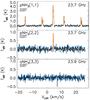 |
Fig. 4 NH3(1,1), (2,2) and (3,3) inversion line spectra observed with the GBT towards the centre of H-MM1. The spectra are on the TMB scale. Fits to the (1,1) and (2,2) hyperfine structures are indicated with orange curves. The origin of the absorption feature seen in the (3,3) spectrum (at 23 869.6 MHz) is unkown to us. |
For other molecules observed here, we use line lists that only take the splitting due to N into account. The data are from Coudert & Roueff (2006) (NHD2 and ND3), and from Caselli et al. (1995), Dore et al. (2004) and Pagani et al. (2009a) (N2H+ and N2D+). The effect of other interactions is likely to be small compared with the thermal broadening (Kukolich 1969; Dore et al. 2004). In the hyperfine fitting, we have assumed that the frequencies listed in Table 1, which are adopted from the CDMS, represent weighted averages of the hyperfine components.
The results of Gaussian fits to the hyperfine structure are presented in Table 3. This table contains the peak main-beam brightness temperatures, TMB, the radial velocities, VLSR, the line widths, Δυ, and the sums of the peak optical thicknesses, τsum, of the hyperfine components. The hyperfine fit also gives an estimate for the Tex of the transition, provided that the spectrum is on the brightness temperature scale. We have approximated this by the TMB scale, which is equivalent to assuming that the source fills the telescope beam uniformly. Finally, the two last columns of Table 3 give the total column densities, Ntotal, of the molecules, and the fractional abundances, X, using the H2 column density derived from Herschel observations. The derived total optical thicknesses of the detected lines range from ~ 1 to ~ 5. This means that the satellites are mainly optically thin, and we are in the regime where the integrated intensity is proportional to the column density of the molecule.
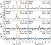 |
Fig. 5 Deuterated ammonia spectra observed at IRAM and APEX. The spectra are presented on the TMB scale. The APEX spectra are Hanning smoothed to a resolution of approximately 0.07 km s-1, which corresponds to the spectral resolution of the spectra from GBT and IRAM. The orange curves are Gaussian fits to the hyperfine structure. |
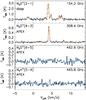 |
Fig. 6 N2D+ and N2H+ spectra observed at IRAM and APEX. The APEX spectra are Hanning smoothed. The velocity resolution is approximately 0.07 km s-1 for the N2D+(2−1) and N2D+(4−3) spectra and approximately 0.1 km s-1 for the higher frequency spectra. Gaussian fits to the hyperfine components of the N2D+(2−1) and N2D+(4−3) lines are shown as orange curves. |
Hyperfine fit results, column densities, and the fractional abundances relative to H2.
While the accuracy of the LSR velocities and line widths from the hyperfine fits is high, the optical thicknesses, and consequently the column densities derived using this method have relatively large uncertainties, except for pNH3 and oNH2D, which are the brightest lines. The oNH2D and pNH2D column densities derived from the lines observed with APEX and IRAM are consistent when the different beam sizes (see Table 2) and the uncertainties owing to noise are taken into account. In contrast, the N2D+ column densities derived from the N2D+(2−1) (IRAM) and N2D+(4−3) (APEX) spectra differ by a factor of five. We consider the value obtained from the N2D+(2−1) spectrum more reliable because this line has several resolved hyperfine components, and because this transition connects rotational levels that are much more densely populated than J = 3 and J = 4. Furthermore, the N2D+ column density obtained from N2D+(2−1) is consistent with that derived from N2D+(1−0) by Punanova et al. (2016) (3.8 ± 0.9 × 1012 cm-2, beamsize 32″) towards a position lying 13″ away from our centre position.
Assuming that ortho- and para-NH3 have equal abundances (which would correspond to their nuclear spin statistical weights), we obtain a total ammonia column density of N(NH3) = (3.3 ± 0.4) × 1014 cm-2. The total column densities for NH2D and NHD2 are N(NH2D) = (1.5 ± 0.1) × 1014 cm-2, N(NHD2) ~ 6.7 × 1013 cm-2. As in the case of NH3, we only detected one spin modification of ND3. Assuming that the relative abundances of ortho-, meta- and para-ND3 correspond to their nuclear spin statistical weights, 16:10:1, we get an estimate for total ND3 column density with large error margins: N(ND3) = (2.7 ± 1.4) × 1012 cm-2. These column density estimates imply the following fractionation ratios: NH2D/NH3 = 0.45 ± 0.09, NHD2/ NH2D ~ 0.45 and ND3/ NHD2 ~ 0.04. The spin ratios can only be estimated for NH2D and NHD2 for which we get o/pNH2D = 3.0 ± 1.1 and o/pNHD2 ~ 1.5. We see that both ortho/para ratios are close to their statistical values, 3 and 2, respectively.
We used the NH3(1,1) and (2,2) maps from GBT to derive the kinetic temperature, Tkin, and the pNH3 column density, N(pNH3), distributions in the vicinity of the H-MM1. The standard analysis described in Ho & Townes (1983), Walmsley & Ungerechts (1983) and Ungerechts et al. (1986) was used. According to the modelling results of Juvela et al. (2012), the ammonia spectra faithfully trace the real mass-averaged gas temperature. In Fig. 7, we show the average N(pNH3) and Tkin as functions of distance from the core centre. The diagrams are derived by averaging spectra over concentric, 10″ wide annuli, and calculating the parameters and their errors from these averaged spectra. Also shown in this figure are the corresponding distributions of N(H2) and TC derived from the Herschel/SPIRE maps. Two things are perhaps worthy of notice in the diagrams: the NH3 abundance seems to decrease and the Tkin seems to increase towards the edge of the core, although both quantities have large errors away from the centre of the core.
The line widths of the spectra observed towards the core centre range from 170 to 260 m s-1. Assuming that the average kinetic temperature in the core is ~ 11 K, the non-thermal velocity dispersions obtained from various transitions are between ~ 50 and ~ 100 m s-1.
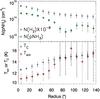 |
Fig. 7 Distributions of the N(NH3) and N(H2) (top) and Tkin and TC (bottom), as functions of the angular distance from the core centre. The N(NH3) and Tkin estimates are derived from the NH3(1,1) and (2,2) maps, whereas N(H2) and TC distributions are based on Hershel/SPIRE far-infrared continuum maps. |
4. Abundances from radiative transfer modelling
4.1. Physical model of H-MM1
In order to account for inhomogeneities in the density and temperature distributions along the line of sight, we constructed a spherically symmetric physical model of the core. Besides providing a realistic description of molecular line excitation conditions for the radiative transfer modelling, the core model is also needed for making a connection between the observations and the theory of interstellar chemistry. In this model, the core structure is described by a modified Bonnor-Ebert sphere (MBES; Evans et al. 2001; Zucconi et al. 2001; Sipilä et al. 2011, 2015c), which is a pressure-bound, hydrostatic sphere of gas and dust with temperature decreasing towards the centre.
We fixed the outer radius of the core to be Rout = 9600 AU (80″). At this distance, the core was assumed to be merged with the ambient cloud. We assumed a constant non-thermal velocity dispersion of σNT = 100 m s-1 inside the core, which increases the internal pressure slightly. The dust temperature profile was calculated using a Monte Carlo program for continuum radiative transfer, CRT6, developed by M. Juvela (Juvela 2005). The spectrum of the unattenuated interstellar radiation field (ISRF) was taken from Black (1994). We used the dust opacity data from Ossenkopf & Henning (1994) for unprocessed dust grains with thin ice coatings7, which agree with the opacities at 250, 350 and 500 μm used in the derivation of the TC and N(H2) maps in Sect. 2.
The MBES model was constructed using the following constraints: 1) the dust temperature at the boundary should agree with the TC outside the core derived from Herschel; 2) the model should approximately reproduce the 450 and 850 μm emission profiles derived from SCUBA-2 maps of Pattle et al. (2015) and 3) the mass-averaged gas kinetic temperature profile, smoothed to the angular resolution of the GBT, should agree with the observed Tkin profile shown in Fig. 7. In order to achieve the large temperature difference between the edge (~ 15 K) and the centre (< 11 K) with the model where the external heating is dominated by the ISRF, we set the visual extinction to AV = 2mag at the outer boundary of the core. With this choice, we assume that the core lies near the edge or in a protrusion of the ambient cloud. The total hydrogen column density in the neighbourhood of the core is of the order of 1022 cm-2 (Fig. 1), which corresponds to AV ~ 10mag. The strongly peaked sub-millimetre emission observed with SCUBA-2 could only be reproduced with central H2 densities of the order of 106 cm-3.
The iteration was started from the density distribution of an isothermal Bonnor-Ebert sphere at 11 K with a central density of n(H2) = 106 cm-3. The intensity of the ISRF and the central density were adjusted to reach agreement with the constraints 1) and 2) above. The sub-millimetre intensity profiles of the model core were calculated by evaluating the integrals 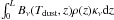 , where the integration is along the line of sight, at different distances from the core centre. The resulting intensity profiles at 450 μm and 850 μm, smoothed to appropriate resolutions, were compared with corresponding circularly averaged profiles from the SCUBA-2 maps.
The gas and dust temperatures are assumed to be equal at densities above ~ 105 cm-3 (Goldsmith 2001). The observed Tkin profile shown in Fig. 7 suggests, however, that the (3-dimensional) gas temperature distribution inside the core does not show the steep gradient characteristic of Tdust caused by the attenuation of the ISRF. In fact, the ammonia observations can be explained with a model where the core is mostly isothermal, but the temperature rises steeply near the edge. We note that this conclusion is probably influenced by the limited angular resolution (cf. temperature determination in L1544 by Crapsi et al. 2007). To conform with the prediction that Tgas ~ Tdust at the highest densities, we assumed that this is true above a certain, adjustable density threshold, but that below this threshold, Tgas is constant up to the transition layer, where it rises abruptly. The adopted gas temperature distribution required a slight adjustment of the density profile to keep the core in hydrostatic equilibrium. The iteration converged after three to four rounds. A reasonable agreement with the dust continuum observations was found with a model where the central density of the core is n(H2) = 1.2 × 106 cm-3 and the standard IRSF is scaled up by the factor 1.7. The observed Tkin distribution could be reproduced assuming that Tgas separates from Tdust at the density n(H2) ~ 4 × 105 cm-3. At this point, ~ 15″ from the centre, the temperature is ~ 11 K.
The distributions of Tgas and Tdust as functions of the radial distance from the core centre for the best fit model are shown in Fig. 8, together with the observable mass-averaged temperature profiles smoothed to the angular resolutions of GBT and Herschel. Figure 9 shows the circularly averaged 450 μm and 850 μm intensity profiles of H-MM1 derived from the SCUBA-2 maps of Pattle et al. (2015), together with predictions from the MBES model.
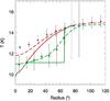 |
Fig. 8 Radial Tdust (red solid curve) and Tgas (green solid curve) distributions of the hydrostatic core model of H-MM1 used in the chemistry modelling and radiative transfer calculations. The corresponding mass-averaged dust and gas temperature profiles are shown as dashed red and green curves. The TC distribution derived from Herschel data is indicated with black plus signs, and the Tkin distribution from the GBT ammonia data is indicated with green diamonds. |
 |
Fig. 9 Sub-millimetre intensities as functions of radial distance from the centre of H-MM1. The plus signs with error bars indicate averages over concentric annuli and their standard deviations. These are obtained from SCUBA-2 maps at 450 μm and 850 μm published by Pattle et al. (2015). The solid curves are predictions from the MBES model described in the text and in Fig. 8. |
4.2. Average abundances from line modelling
We derived the fractional abundances of the observed molecules in H-MM1 by applying the Monte Carlo radiative transfer program of Juvela (1997) to the physical model described in Sect. 4.1. The collisional rate coefficients for NH2D were adopted from Daniel et al. (2014), and for NHD2 and ND3 we used the newly calculated coefficients from Daniel et al. (2016b). For N2D+, we used the collisional rate coefficients for N2H+ from the recent work of Lique et al. (2015).
In this calculation, we assumed constant fractional abundances throughout the core, that is, that there is no dependence on the distance from the core centre. The obtained values can thus be taken as averages over the core. Starting from the estimates presented in Table 3 of Sect. 3, we varied fractional abundances until the modelled spectra produced the same integrated intensities as the observed ones. The best-fit fractional abundances are presented in Table 4. The uncertainties correspond to the 1σ errors of the integrated intensities. The para-NH3 lines are broader than those of its deuterated isotopologues, and for this molecule we had to increase the assumed non-thermal velocity dispersion to σNT = 150 m s-1 in order to reproduce the integrated intensities. This suggests that NH3 emission has contribution from the ambient cloud having a larger velocity dispersion than the core, and that the derived fractional para-NH3 abundance is an upper limit for the core.
For the different isotopologues of ammonia, the agreement reached between the predicted spectra and observations is equally good as for the hyperfine fits shown in Figs. 4 and 5. The two N2D+ lines detected cannot be reproduced by a single abundance. The value listed in Table 4 is a compromise that over-predicts the N2D+(4−3) intensity but gives an overly weak N2D+(2−1) line. The situation is thus opposite to what is expected from the results of the hyperfine fits. This indicates that either the assumption of a constant abundance is unrealistic for N2D+ or that the physical model is inaccurate.
Fractional abundances, deuterium fractionation ratios, and spin ratios in H-MM1 derived from the detected lines using radiative transfer modelling.
The abundances listed in Table 4 imply the following total fractional abundances: X(NH3) = (7.6 ± 0.1) × 10-9 (assuming o:p=1:1), X(NH2D) = (2.9 ± 0.1) × 10-9, X(NHD2) = (6.4 ± 0.5) × 10-10 and X(ND3) = (3.7 ± 0.4) × 10-11 (assuming o:m:p = 18:10:1). Here we have assumed statistical spin ratios for species without a line detection. The corresponding deuterium fractionation ratios for ammonia, and the ortho/para ratios for NH2D and NHD2 are listed in the bottom part of Table 4.
For the molecules with the brightest lines, the abundances from the radiative transfer modelling agree relatively well with those from the LTE analysis (Table 3). The most glaring discrepancy (by a factor of 2.5) is found for para-NHD2 with the weakest detection and a very large uncertainty of the optical thickness from the LTE method. The statistical errors of the fractional abundances listed in Table 4 are small in most cases, but the values are subject to systematic errors depending on accuracy of the physical model, and on the validity of the assumption of constant abundances. The present physical model is, however, consistent with dust continuum observations, and provides a more realistic description of the excitation conditions in the core than the assumption of line-of-sight homogeneity. Therefore, we consider the abundance ratios listed in Table 4 to be more accurate than those implied by the values presented in Table 3, and use the former ratios to assess the validity of the chemistry model described below.
5. Chemical modelling
5.1. Model description
We model the chemistry of H-MM1 using the pseudo-time-dependent gas-grain chemical code presented in earlier papers (Sipilä 2012; Sipilä et al. 2013, 2015a,b) where the details of the code (e.g., the expressions of the various reaction rate coefficients) can be found. The model includes gas-phase chemistry, adsorption onto and (non-thermal) desorption from grain surfaces, and grain-surface chemistry. Tunnelling diffusion of H and D atoms on grains is not considered in the present calculations, whereas tunnelling through activation energy barriers in surface reactions has been included.
The program can be instructed to include various desorption mechanisms: thermal desorption (negligible in the physical conditions explored here), cosmic ray desorption, reactive desorption and photodesorption. Cosmic ray desorption is treated following Hasegawa & Herbst (1993). Exothermic association reactions on the surface can result, when this option is turned on, in desorption of the reaction product with an efficiency of 1% (Garrod et al. 2007). Finally, it is possible to include photodesorption of water, CO and ammonia caused by secondary UV photons created by H2 excitation (Prasad & Tarafdar 1983). In the simulations presented here, however, the photodesorption and reactive desorption options have been turned off. According to extensive testing, the inclusion of these processes increases the ammonia production, which in turn makes it necessary to lower the elemental N abundance to ensure compliance with the observed line intensities, but fractionation and spin ratios remain largely unchanged.
The spin-state chemical model presented in Sipilä et al. (2015a) describes the spin states of species involving multiple protons. Recently, we upgraded this model to include a self-consistent description of the spin states of multiply-deuterated species (Sipilä et al. 2015b). This is achieved by considering nuclear spin selection rules arising from molecular symmetries, assuming full scrambling of nuclei in reactive collisions. The model gives the necessary information for the present application, that is, the calculation of simulated line emission from deuterated ammonia. In the beginning of the simulation, all elements are in the atomic form, with the exceptions of hydrogen and deuterium, which are initially locked in H2 and HD, respectively.
The descriptions of deuterium and spin-state chemistry adopted here apply to both gas-phase chemistry and grain-surface chemistry. However, the formation mechanism of ammonia (as a particular example) is different in the gas and on the grains. In the gas phase, (deuterated) ammonia forms through a network of ion-molecule reactions, while on the surface, the formation mechanism is hydrogen/deuterium addition. Therefore we expect non-statistical deuterium and spin-state ratios in the gas phase, and statistical ratios on the grain surface, although complete scrambling is assumed in both cases. The assumed binding energies on grain surfaces are the same as listed in Table 2 of Sipilä et al. (2015a).
For the elemental abundances, we have adopted the set of low-metal elemental abundances labelled EA1 in Wakelam & Herbst (2008), except for the nitrogen abundance for which we needed to increase the EA1 abundance by a factor of 2.5 to N/H = 5.3 × 10⁻⁵ to reproduce the observed line intensities of NH2D, NHD2, ND3 and N2D+. According to the recent compilation of Jenkins (2009), the appropriate value for the diffuse ISM is N/H = 6.2 × 10⁻⁵. The adopted carbon and oxygen abundances are O/H = 1.8 × 10⁻⁴ and C/H = 7.3 × 10⁻⁵.
We derive abundance profiles for the various molecules by separating the core model (see Sect. 4.1) into a series of concentric spherical shells, each associated with unique values of density, gas/dust temperatures and visual extinction AV. Chemical evolution is then calculated separately in each shell, which leads to simulated abundances for each chemical species as functions of time and radial distance from the core centre. The integration of the modelled abundance gradients into the radiative transfer model is discussed in Sect. 5.3.
5.2. Chemical evolution of the core
We calculate the evolution of chemical abundances in the core model with the aim being to examine if the model can reproduce, at a certain stage of the simulation, the intensities of the lines of deuterated ammonia and N2D+ observed towards H-MM1 in the present study, as well as the intensities of the oH2D+ and pD2H+ lines observed previously by Parise et al. (2011).
We assume that the spin temperature of H2 has been thermalised during the initial contraction phase of the cloud down to ~ 20 K (Flower et al. 2006b; Sipilä et al. 2013), and accordingly, set the initial o/pH2 to 1 × 10⁻³. For the cosmic ray ionisation rate of H2, we assume ζH2 = 1.3 × 10⁻¹⁷ s-1, and the average grain radius is set to a = 0.1 μm. These are kept unchanged in the present simulations. We note, however, that deuteration can be delayed by increasing the initial o/pH2 ratio, and that the fractionation ratios can be lowered by decreasing the average grain size or by increasing the cosmic ionisation rate (Sipilä et al. 2010). On the other hand, an increase of the cosmic ray ionisation rate would generally increase the abundances and the line intensities of  , NH3 and their deuterated isotopologues, and decrease the abundances and line intensities of N2H+ and N2D+.
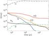 |
Fig. 10 Fractional abundances of selected species relative to H2 as functions of time in the core model described in Sect. 4.1. The abundances are density weighted averages. |
We first discuss the predictions for some of the most common species. The gas-phase abundances of the H, D and N atoms, and the HD, CO and N2 molecules, relative to the total hydrogen abundance, are plotted in Fig. 10, as functions of time for our fiducial core model discussed in Sect. 4.1. The abundances are averages over the line of sight through the centre of the core, weighted by the density. The freeze-out of CO is followed by an increase of , which in turn results in an enhanced ortho-para conversion of H2. At the same time, deuterium is efficiently transferred from HD to deuterated ions in the gas phase (to H2D+, D2H+ and  in the first place). The H and D atoms released in the dissociative recombination of deuterated ions mainly accrete onto grains, where they can combine to give back H2 or HD, but also react with heavier atoms or radicals. At late stages of chemical evolution, deuterium becomes increasingly incorporated into icy compounds. In the gas phase, this is reflected by the reduction of the HD abundance.
The rapid decrease of atomic nitrogen at the beginning of the simulation is mainly caused by accretion onto grains. A fraction of the nitrogen atoms in the gas phase is converted to N2 through N + OH → NO + H, N + NO → N2 + O (Flower et al. 2006a; Le Gal et al. 2014). This reaction is important at early times, when the N and OH abundances are high. Also, the N2 molecules accrete onto grains, but their desorption from grains is more significant than for N atoms, which quickly react with other atoms or radicals, for example, N∗ + H∗ → NH∗, N∗ + O∗ → NO∗ or  . Species attached to grains are indicated here with asterisks. The surface species
  is destroyed by only two processes; desorption or photodissociation,
  , by cosmic-ray induced UV photons. This is the main difference from CO∗ for which hydrogenation, CO∗ + H∗ → HCO∗, competes strongly against desorption (see also Sect. 6.1).
Owing to desorption, the N2 abundance remains high in the gas phase until late stages of the simulation. Molecular nitrogen is prerequisite to N2H+, which forms through 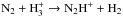 . In case reactive desorption is included, the most important source of ammonia at very early stages of simulation is formation on grains,
  , where ammonia is supposed to be released into the gas phase at the probability of 1%. After a few thousand years, gas-phase formation takes over. In the simulations presented here, the ammonia production is always dominated by the well-known chain of gas-phase reactions, terminating in
 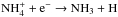 (e.g. Le Gal et al. 2014; Roueff et al. 2015). As discussed by Sipilä et al. (2015b), the dissociative ionisation of HNC by He+ helps the initiation of this chain by producing NH+, which would otherwise be solely dependent on N+ + oH2 → NH+ + H (Dislaire et al. 2012).
The evolution of the abundances of NH3 and N2H+ as well as their deuterated isotopologues in the gas phase are shown in Fig. 11 (top panel). The other two panels show the fractionation ratios and the spin ratios for these species. In Fig. 12, we show the abundances, fractionation ratios and the spin ratios of the grain-surface species  , NH2D∗,
  and
and  . The middle panel of this latter figure also shows the atomic D∗/H∗ on grains.
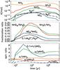 |
Fig. 11 Gas-phase fractional abundances of NH3 and N2H+ and their deuterated isotopologues as functions of time in the core model. The N2D+/ N2H+ and m/pND3 ratios are divided by 10 to make the other ratios readable in these diagrams. |
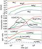 |
Fig. 12 Evolution of the abundances of NH3 and its deuterated isotopologues on grain surfaces for the core model. The m/pND3 ratios are divided by 10. The D/H ratio on grains shown in the middle panel is multiplied by 0.2. |
In the present model, the gas-phase NH3 abundance is built up early and does not change significantly at later times. The largest variations are seen in the abundances of NHD2, ND3 and N2D+, which grow rapidly in the beginning, and decay slowly after the deuteration peak. This behaviour seems to reflect the variations in the D2H+ and abundances that are shown in Fig. 13. The ion reaches its maximum before D2H+, which in turn peaks before H2D+. Likewise, the maximum fractionation ratio ND3/ NHD2 occurs earlier than the maximum in the NHD2/ NH2D ratio, which again takes place long before the NH2D/NH3 peak.
In the bottom panel of Fig. 11, one can see that while the o/p-NH2D ratio decreases slightly with time, o/p-NHD2, m/p-ND3 and m/o-ND3 have increasing tendencies. The predicted ratios are close to their statistical values in the beginning of the simulation. The o/p-NHD2 and m/p-ND3 ratios mimic the corresponding ratios of D2H+ and shown in Fig. 13, bottom panel. The relationship between the spin modifications of NH3 and is discussed in Sect. 6.
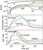 |
Fig. 13 Evolution of the isotopologues of |
The ammonia production on grain surfaces is very efficient in the present model. The deuteration of ammonia occurs more slowly than in the gas phase, and never reaches fractionation ratios as large as those seen there. The spin ratios on grains stay close to their statistical values at all times, except that m is enhanced at the cost of o and p.
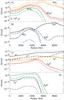 |
Fig. 14 Fractional abundances of selected species as functions of the radial distance from the core centre at the time 3 × 10⁵ yr from the beginning of the simulation. The abundances of ortho species are drawn with solid lines, and those of para species are drawn with dashed lines. The abundances of meta species (ND3 and |
5.3. Predicted spectra
The radial distributions of the density, temperature and the (time-varying) chemical abundances in the gas phase are used as input for a Monte Carlo radiative transfer program (Juvela 1997) to predict observable rotational line profiles. As in simulations described in Sect. 4.2, we use a larger non-thermal velocity dispersion (σN.T. = 150 ms-1) for NH3 than for the deuterated species (for which σN.T. = 100 ms-1) in order to reach agreement with the observed integrated intensities.
The line intensities depend, besides the (mass averaged) abundances of the species within the telecope beam, on their radial distributions, which change with time. At early stages, deuterated species are concentrated on the core centre with high densities, whereas later on, when freezing onto grains reduces the abundances in the centre, line emission is dominated by lower-density outer parts of the core. The changes of the abundance profiles mean that at early times, lines with large transition dipole moments, such as N2D+(4−3) and mND3(10−00), are much stronger than the o/pNH2D(111−101) lines, for example; the reverse is true at later times, however. The fractional abundances of selected species as functions of the radius are shown in Fig. 14. The distributions are taken at the time when most of the predicted spectra agree reasonably well with the observations.
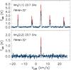 |
Fig. 15 NH3(1,1) and (2,2) spectra produced by the core model at t = 3 × 10⁵ yr (red curves) together with the observed spectra (histograms). The model over-predicts the observed intensities. The model agrees with observations at t = 105 yr and t = 2 × 10⁶ yr. The intensities are given on the main-beam brightness temperature (TMB) scale. |
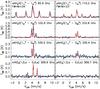 |
Fig. 16 Deuterated ammonia spectra produced by the core model at t = 3 × 10⁵ yr (red curves) together with the observed spectra (histograms). |
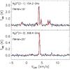 |
Fig. 17 Modelled and observed N2D+(2−1) and N2D+(4−3) spectra on the TMB scale. The modelled spectra are predictions for 3 × 10⁵ yr (red curves) after the beginning of the simulation. |
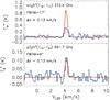 |
Fig. 18 Comparison between the observed (black histograms) and modelled (red curves) oH2D+(110−111) and pD2H+(110−101) spectra as observed with APEX. The observations are from Parise et al. (2011). The spectra are on the |
The intensities of the simulated NH2D, NHD2, ND3 and N2D+ spectra are comparable with those of the observed ones during rather a short period around the NHD2/ NH2D peak, occurring at ~ 3 × 10⁵ yr from beginning of the simulation. At this time, however, the predicted beam-averaged pNH3 abundance, X(pNH3) ~ 5 × 10⁻⁹, is approximately 30% higher than needed to reproduce the NH3(1,1) and (2,2) line intensites observed at the GBT (see Table 4). The simulated NH3 lines agree with the observed ones at an early stage, around 105 yr, and much later, around 2 × 10⁶ yr, when ammonia depletion has finally started to take effect. The predicted spectra at t = 3 × 10⁵ yr are shown in Figs. 15 (NH3), 16 (NH2D, NHD2 and ND3), 17 (N2D+) and 18 (oH2D+ and pD2H+).
The model predicts that the abundances of the different isotopologues of NH3 and N2H+ grow at different rates. This implies that the fractionation ratios, NH2D/NH3, NHD2/ NH2D, ND3/ NHD2, do not necessarily reach their maxima at the same time. This is illustrated in the middle panel of Fig. 11. In this model, the peak fractionation ratios range from 0.15 to 0.30, depending on the pair of species considered. The ND3/ NHD2 ratio mimics the N2D+/ N2H+ ratio divided by 10, and these two fractionation ratios are the first to peak in all the models we have run. This tendency is related to the rapid growth of the abundance occurring at early stages of the simulation (Fig. 13). The fact that the average temperature exceeds 10 K has a favourable effect on deuteration, but its fast advancement is made possible by the low initial o/pH2 ratio assumed in the simulation. A higher abundance of oH2 would delay the deuterium peak by obstructing the primary deuteration through reaction  (Flower et al. 2006b; Pagani et al. 2011, 2013; Kong et al. 2015).
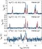 |
Fig. 19 Observed (black histograms) and modelled (red curves) N2H+(1−0), N2D+(1−0), and C17O(1−0) spectra as observed with IRAM 30-m. The observations are from Punanova et al. (2016). The spectra are on the TMB scale. The model spectra correspond to the time 3 × 10⁵ yr in the simulation. |
In Figs. 18 and 19, we compare our model predictions with the previous observations of Parise et al. (2011) and Punanova et al. (2016). The modelled oH2D+(110−111) and pD2H+(110−101) spectra shown in Fig. 18 are on the  scale as observed with APEX to allow comparison with the spectra shown in Fig. 3 of Parise et al. (2011). These spectra are reproduced in Fig. 18. The 13″ offset from the supposed core centre position is taken into account. The hyperfine patterns of the lines have been adopted from Jensen et al. (1997). The line profiles are dominated, however, by the thermal broadening. While the simulated pD2H+ line approximately agrees with the observations, the simulated oH2D+ line is brighter than the observed one by a factor of three. A good agreement with both observations would be found at very early times by setting the initial o/pH2 ratio to 10-4. On the other hand, that model cannot reproduce the observed line ratios for the other molecules. After t ~ 4 × 10⁵ yr, the pD2H+ line intensity decreases rapidly below the observed
  K while oH2D+ remains relatively strong. This behaviour is determined by the close correlation between o/pH2D+ and o/pH2, and the increase of the o/pD2H+ ratio with time (Fig. 13).
The N2H+(1−0), N2D+(1−0), and C17O(1−0) spectra observed at the IRAM 30-m telescope by Punanova et al. (2016) are shown in Fig. 19 together with the predicted spectra at the time 3 × 10⁵ yr. The H-MM1 spectra of Punanova et al. (2016) were obtained towards the (0, 0) of Parise et al. (2011), and also here the 13″ offset from the core centre is taken into account. The model reproduces the observed N2D+(1−0) spectrum reasonably well, but gives a vastly undervalued C17O(1−0) intensity. According to the model, CO is heavily depleted in the core at the time 3 × 10⁵ yr (Fig. 10). The peak velocity and velocity dispersion of the observed C17O(1−0) line are, however, different from those of the N2H+ and N2D+ lines. The C17O emission is probably dominated by the ambient cloud, which is not included in our model. Also the shape of the N2H+(1−0) line suggests that part of the emission originates in the ambient cloud. According to the radial abundance distributions shown in Fig. 14, N2H+ belongs to species that are not confined to the core. Nevertheless, the model seems to under-predict the N2H+(1−0) emission from the core.
To summarise comparisons with observations, the core model predicts the observed intensities of the N2D+, NH2D, NHD2, ND3 and para-D2H+ lines rather well, overproduces para-NH3 and ortho-H2D+ and gives overly low N2H+(1−0) and C17O(1−0) line intensities. Besides these discrepancies, the present model has problems in reproducing the observed spin ratios. Inspection of Fig. 16 reveals that the model underestimates the o/pNH2D ratio and overestimates the o/pNHD2 ratio.
6. Discussion
6.1. Ubiquity of ammonia
Our chemical network predicts that the ammonia abundance builds up quickly in the gas phase. The predicted fractional abundances are similar to those found previously in molecular clouds, in particular, in the Ophiuchus complex (Friesen et al. 2009), even though the model over-predicts the pNH3 abundance in H-MM1 during the deuteration peak. During the very beginning of the simulation, the production is dominated by surface reactions followed by desorption, but after a few thousand years, ion-molecule reactions in the gas phase take over as the main source of gaseous ammonia. At early stages, the rapidly evolving carbon chemistry comes to aid as the dissociative ionisation reaction HNC + He+ provides a short cut to NH+, past the slow formation of N2 and the famous bottle-neck reaction N+ + H2.
The ammonia abundance remains high until very late stages of the simulation. One of the reasons is the slow decrease of the molecular nitrogen abundance, which is sustained by desorption. In this respect, N2 acts differently from CO, which freezes out quickly. In the presence of and H+, N2 replenishes the gas with the NH+ ion through the sequence 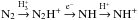 . NH+, in turn, fuels the ammonia production through successive reactions with H2 (see, e.g. Flower et al. 2006a; Le Gal et al. 2014).
In the present model, N2 attached to a grain can either photodissociate or be desorbed. N2 and CO, even if isoelectronic, have very different surface chemistries. The two molecules have approximately the same adsorption energies on amorphous ice: approximately 1100 K for CO and approximately 1000 K for N2 (Hama & Watanabe 2013; Fayolle et al. 2016). Hydrogenation of CO (CO∗ → HCO∗ → H2CO∗ → H3CO∗ → H3COH∗) has been experimentally observed and characterised (Hama & Watanabe 2013, and references therein) at temperatures down to 3 K, where the intermediate HCO could be detected (Pirim & Krim 2011). The reaction CO + H → HCO proceeds by tunnelling through an activation barrier computed to be approximately 2000 K in the gas phase, and probably lower on the surface of amorphous ice (Peters et al. 2013; Rimola et al. 2014). The exothermicity of the reaction is approximately 6700 K, while the endothermicity of the reaction CO + H → COH is approximately 10 000 K (Zanchet et al. 2007; note that this theoretical paper overestimates the exothermicity of the reaction leading to HCO). The case of N2 is different: the reaction N2 + H → N2H is endothermic by approximately 4400 K (Bozkaya et al. 2010) and does not occur on ice surfaces. The neutral chemistry of CO and N2 proceeds thus in very different ways, with no surface hydrogenation of N towards ammonia NH3 or hydrazine N2H4. However, the ionic chemistry on low-temperature ice surfaces is not fully characterised.
6.2. Fractionation ratios
The abundance of NH2D starts to increase gradually, first through the deuteron transfer to ammonia, primarily by HCND+ or DCNH+, e.g. HCND+ + NH3 → NH3D+ + HCN, followed by dissociative recombination of NH3D+. The depletion of CO boosts the abundance of , which in turn is efficiently deuterated to H2D+, D2H+ and in successive reactions with HD. This stage is characterised by a rapid increase of NHD2, ND3 and N2D+. The most important reactions contributing to the formation of NH2D during the deuteration peak are shown in Fig. 20. These comprise the deuteron transfer from H2D+, or some other deuterated ion, to NH3 giving NH3D+, dissociative recombination of NH3D+, charge transfer between NH2D and H+ and hydrogen abstraction from H2 to the NH2D+ ion.
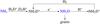 |
Fig. 20 Principal reactions forming and destroying NH2D at the deuteration peak. |
Characteristic of the reaction scheme is the circulation between neutral and ionic species generated by the charge transfer reaction with H+, one of the ions which increases in number after the disappearance of CO. Precursors of doubly and triply deuterated ammonia,  and
and  , are mainly formed from reactions between NH3 and D2H+ or in the present model. This reaction network is discussed in more detail in Sipilä et al. (2015b).
The N2D+ ion, which is mainly produced in reactions between N2 and H2D+, D2H+ or , is strongly favoured by the successive deuteration of . At the time of the most vigorous deuteration, the NH3 abundance decreases slightly owing to accretion onto grains and enhanced charge exchange reactions caused by the increase of H+. After that, until very late times, probably exceeding the lifetime of the core, the NH3 abundance remains almost constant, and so does the abundance of NH2D. In contrast, the abundances of NHD2, ND3, N2H+ and N2D+ rise and fall in the time range shown in Fig. 11. At late times, these species are most strongly influenced by the depletion of nitrogen and deuterium in the gas phase.
The best overall agreement between the modelled and observed NH2D, NHD2 and ND3 spectra is achieved at t ~ 3 × 10⁵ yr. At this stage of the model, the fractionation ratios are NH2D/NH3 ~ 0.25, NHD2/ NH2D ~ 0.25 and ND3/ NHD2 ~ 0.1 (while the observed fractionation ratios are NH2D/NH3 ~ 0.4, NHD2/ NH2D ~ 0.2 and ND3/ NHD2 ~ 0.06). The time is coincident with the NHD2 maximum, whereas ND3 is already decreasing at that time. The obtained fractionation ratios are reasonably close to what was found in previous observational studies (Roueff et al. 2005; Daniel et al. 2016b), but it should be noted that our results suggest that large temporal variations are possible, also when the physical conditions remain constant. The spectral line simulations show that all three deuterated forms of ammonia should be easily detectable from a core such as H-MM1 even if the fractionation ratios were reduced to half of those derived here. In particular, the early formation of ND3 and the large transition dipole moment of the rotation-inversion transition of mND3 at 309.9 GHz makes this line a useful signpost of the deuterium peak.
According to the present chemistry model, the fractionation ratios on grain surfaces are lower than those in the gas phase by a factor of two. The atomic D∗/H∗ ratio on the grain surfaces, which determines the overall degree of deuteration there, reaches a high value of ~ 0.4 a little before 105 yr in the present simulation (Fig. 12). Because of competition between various viable addition reactions for H∗ and D∗ (for example with NO∗, HCO∗ and HS∗), the abundances of deuterated forms of ammonia build up slowly. Towards the end of the simulation, the abundances settle, however, almost exactly to the values expected from the statistical rule 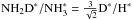 ,
,  ,
,  , as predicted by Brown & Millar (1989).
6.3. Spin ratios
In the gas phase, the ortho/para ratio of NH2D is largely determined by the cycle consisting of reactions with H+, H2 and e− shown in Fig. 20. In the present chemistry model, full scrambling of H nuclei is assumed to take place in these reactions, and, owing to nuclear spin selection rules, o/pNH2D should settle to approximately 2.3 (Sipilä et al. 2015b). The full reaction set predicts that the ratio decreases to approximately 2.0 at late times (Fig. 11).
Similar cycles involving NHD2 and ND3 preserve the spin states of D2 and D3. Consequently, the spin ratios of doubly and triply deuterated ammonia are determined by the primary deuteration reactions D2H+ + NH3 and  . The reaction scheme is discussed in detail in Sipilä et al. (2015b). The fact that o/pNHD2 follows o/pD2H+ closely can be seen in Figs. 11 and 13. A tight correlation between m/p-ND3 and m/p- is also evident from these figures.
By comparing the modelled and observed spectra shown in Fig. 16, one finds that while the modelled o/pNH2D ratio is too low, the corresponding ratio for NHD2 is too high. The discrepancy is more pronounced in the case of pNHD2 for which the predicted spectrum underestimates the observed intensity by approximately 40%. As mentioned in Sect. 5.2, the timing and the strength of the deuterium peak can be affected by the selection of the initial o/p-H2 ratio, the cosmic ray ionisation rate and the average grain size, but these modifications do not change the fact that the o/pNHD2 ratio given by our model during the deuterium peak is larger than the observed ratio. If the adopted deuteration scheme is correct, the implication is that also the o/pD2H+ ratio is overestimated in the model, because o/pNHD2 is directly related to o/pD2H+.
However, the spin ratio of D2H+ is determined by the well-studied  isotopic system (Hugo et al. 2009), and the prediction of a high o/pD2H+ ratio seems to be well-founded. The lower energy, ortho form of D2H+ is favoured over pD2H+ both in the primary production through H2D+ + HD → D2H+ + H2 and in the “backward” reactions
  and o/pD2H+ + oH2 → o/pH2D+ + HD. In addition, para - ortho conversion of D2H+ is viable in cold clouds through reaction with HD (see discussion in Flower et al. 2006b; and Sipilä et al. 2010).
6.4. Statistical abundance ratios
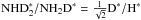
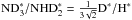
In their analysis of the deuterated ammonia observations towards Barnard 1 and L1689N, Daniel et al. (2016b) concluded that the observational data (considering the error margins) are consistent with the assumption that both the fractionation ratios and the spin ratios are equal to the corresponding statistical ratios. Daniel et al. (2016b) point out that statistical fractionation and spin ratios would be expected if the production of ammonia molecules were dominated by surface reactions. On grain surfaces, where ammonia formation takes place through H/D atom additions to N, the fractionation ratios, NH2D/NH3, NHD2/ NH2D and ND3/ NHD2, should successively diminish by a factor of three (Brown & Millar 1989; Rodgers & Charnley 2001), and the spin ratios should follow the ratios of the corresponding nuclear spin statistical weights.
Also in the present study, the nuclear spin ratios derived directly from the observed lines agree with their statistical values, and NHD2/ NH2D ~ 3ND3/ NHD2 as expected from combinatorial principles (see Table 4 in Sect. 4.2). The NH2D/NH3 ratio falls, however, below the value expected from the other two fractionation ratios. On the other hand, the derived NH3 abundance for the core may be an overestimate as discussed in Sect. 4.2.
The observed spectra originate, however, in the gas phase, and also sublimated species are likely to be exposed to rapid processing by ion-molecule reactions there. The fractionation ratios on grain surfaces depend on the atomic D∗/H∗ ratio on grains, which, according to the present simulation, is, at any time, much higher than the atomic D/H ratio in the gas phase (Figs. 10 and 12). As mentioned in Sect. 6.2, the statistical fractionation ratios for ammonia on grains are only reached at very late times of the simulation.
The observations suggest, therefore, that the adopted gas-phase deuteration scheme for ammonia (illustrated in Fig. 2 of Sipilä et al. 2015b) is not correct. The model assumes complete scrambling of H or D nuclei in the intermediate reaction complexes. This assumption is highly uncertain for several reactions involved in the production of ammonia (Rist et al. 2013).
An argument against a full scrambling of the reaction forming the ammonium ion,  , comes from the energetics of this reaction (an intermediate reaction complex is indicated here with ()‡). The reaction is likely to occur through two minima on the potential energy surfaces,
  and (NH4··H+)‡. According to the calculations of Ischtwan et al. (1992), some of the conceivable interchanges of two H nuclei between different parts of these complexes are facile, but most of them involve high energy
  transition states with different geometries. The D-substituted cases should be very similar. However, since it is known experimentally that, for example, D/H exchange occurs between
  and D2, Ischtwan et al. (1992) proposed that it is possible to circumvent a high-energy transition state by a process where hydrogen transfer is followed by internal rotation and reverse transfer. In none of the configurations of do all H (or D) nuclei occupy equivalent positions. Consequently, the spin symmetry rules for this reaction are far from obvious, even less so given that internal rotations are likely to occur.
For the reaction NH3 + H2D+ and its doubly deuterated analogue (Fig. 21 below), the situation is even less clear. While the reaction proceeds at 30 K (Lindinger et al. 1975; Marquette et al. 1989), there is no theoretical computation on the (NH5D+)‡ complex; see for example Rist et al. (2013). There is no current experimental or theoretical discrimination between scrambling or proton hop mechanisms for this reaction.
In the present model, we assume that the reaction NH3 + D2H+ forms the complex  , which can dissociate to
  , NH3D+ or . If this is true, the reaction is one of the main sources of NHD2. If the reaction complex is not formed, but D2H+ simply donates the proton or one of the deuterons to ammonia, the outcome after dissociative recombination could be either NH3 or NH2D, as illustrated in Fig. 21. The statistical branching ratios are indicated in this figure.
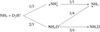 |
Fig. 21 Branching ratios of the reaction NH3 + D2H+ assuming that this can be described as proton/deuteron hop. |
It seems that several important reactions, which in the model have been assumed to proceed through long-lived intermediate complexes where nuclei can be scrambled, should rather be described as proton/deuteron hops or hydrogen/deuterium abstractions. In these reactions, H and D nuclei are effectively added one by one, as in surface reactions, and they produce each nuclear spin modification according to its statistical weight.
The assumption that ammonia is primarily processed in reactions with the isotopologues of , such as the one described in Fig. 21, can eventually lead to a ratio of 3 between successive levels of deuteration, although now the fractionation ratios would not depend on D/H nor D∗/H∗, but on the relative abundances of , H2D+, D2H+ and . Using combinatorics, one can show that in steady state NH2D/NH3 = 3γ, NHD2/ NH2D = γ, and  , where
 ![Mathematical equation: \begin{eqnarray*} \gamma=\frac{[\htwod]+2[\dtwoh]+3[\dthree]}{3[\hthree]+2[\htwod]+[\dtwoh]}\cdot \end{eqnarray*}](/articles/aa/full_html/2017/04/aa28463-16/aa28463-16-eq395.png) Nyman (2016) has recently discussed a simple statistical model for the deuteration of interstellar ammonia that neglects the reaction kinetics. In its simplest form, this model leads to the same rule for the fractionation ratios, NH2D/NH3 = 3 NHD2/ NH2D = 9 ND3/ NHD2, as the models discussed above, but now the parameter γ = NHD2/ NH2D depends on the elemental N/D ratio through γ = 1/(3 N/D−1). The fractionation ratio NHD2/ NH2D ~ 0.2 observed in H-MM1 and in L1689N (Roueff et al. 2005) would imply N/D ~ 2, which is approximately 30% lower than the ratio assumed in the chemistry model used here. The inclusion of energetics into this model through the molecular partition functions makes the fractionation ratios correspond to what would be obtained at LTE, giving NH2D/NH3 ≤ NHD2/ NH2D. While this agrees with the earlier results presented in Roueff et al. (2005), the fractionation ratios found in the present study, and in the re-analysis of the B1b results by Daniel et al. (2016b), suggest NH2D/NH3 ~ 2−3 NHD2/ NH2D. Therefore, the assumption of thermal equilibrium between different deuterated isotopologues of ammonia does not seem to be universally valid. This situation is also unlikely because large deviations from thermal equilibrium are usually found in cold interstellar gas. On the other hand, as recommended by Nyman (2016), the energetics, and especially the differences in the vibrational zero-point energies between different ammonia isotopologues, should be taken into account in kinetic models. This would particularly affect reactions working against deuteration.
Nyman (2016) has recently discussed a simple statistical model for the deuteration of interstellar ammonia that neglects the reaction kinetics. In its simplest form, this model leads to the same rule for the fractionation ratios, NH2D/NH3 = 3 NHD2/ NH2D = 9 ND3/ NHD2, as the models discussed above, but now the parameter γ = NHD2/ NH2D depends on the elemental N/D ratio through γ = 1/(3 N/D−1). The fractionation ratio NHD2/ NH2D ~ 0.2 observed in H-MM1 and in L1689N (Roueff et al. 2005) would imply N/D ~ 2, which is approximately 30% lower than the ratio assumed in the chemistry model used here. The inclusion of energetics into this model through the molecular partition functions makes the fractionation ratios correspond to what would be obtained at LTE, giving NH2D/NH3 ≤ NHD2/ NH2D. While this agrees with the earlier results presented in Roueff et al. (2005), the fractionation ratios found in the present study, and in the re-analysis of the B1b results by Daniel et al. (2016b), suggest NH2D/NH3 ~ 2−3 NHD2/ NH2D. Therefore, the assumption of thermal equilibrium between different deuterated isotopologues of ammonia does not seem to be universally valid. This situation is also unlikely because large deviations from thermal equilibrium are usually found in cold interstellar gas. On the other hand, as recommended by Nyman (2016), the energetics, and especially the differences in the vibrational zero-point energies between different ammonia isotopologues, should be taken into account in kinetic models. This would particularly affect reactions working against deuteration.
7. Conclusions
Ammonia and its three deuterated isotopologues were detected towards the starless core H-MM1 in Ophiuchus. By modelling the observed spectra, we derived the following fractionation ratios: NH2D/NH3 ~ 0.4, NHD2/ NH2D ~ 0.2 and ND3/ NHD2 ~ 0.06. The relative line intensities of the ortho and para modifications of NH2D and NHD2 are consistent with the statistical spin ratios o/pNH2D = 3 and o/pNHD2 = 2. The fractionation and spin ratios are similar to those obtained towards two young cores (L1689N and B1), which are the only objects previously observed in all four molecules (Roueff et al. 2005; Roueff et al. 2015; Daniel et al. 2016b).
The observations towards H-MM1 were simulated using a gas-grain chemistry model in conjunction with a Monte Carlo radiative transfer program. In the chemistry model, which includes cosmic-ray-induced desorption and tunnelling through activation energy barriers in surface reactions, ammonia forms early and stays long in the gas phase. The model over-predicts pNH3 and oH2D+, but can approximately reproduce the observed NH2D, NHD2, ND3, N2D+ and pD2H+ lines. The oH2D+ and pD2H+ observations used here are from Parise et al. (2011). According to the simulation, the longevity of NH3 and N2H+ in the gas phase can be traced back to the chemical inertness of N2 on the grain surfaces. Unlike CO, the nitrogen molecule is not supposed to be hydrogenated on grain surfaces, which makes it susceptible to desorption.
The present chemistry model cannot account for the observed o/pNH2D and o/pNHD2 ratios satisfactorily. In conditions prevailing in H-MM1 and in other starless, dense cores, characterised by low temperature, high obscuration and inefficient desorption, the spin ratios should be determined by gas-phase ion-molecule reactions. When complete scrambling of H and D nuclei in these reactions is assumed, the spin ratios are predicted to settle to o/pNH2D ~ 2 and o/pNHD2 ~ 3−4 by the time all three deuterated forms of ammonia become detectable, instead of their statistical ratios 3 and 2, respectively. The fact that the observed spin ratios nevertheless correspond to the nuclear spin statistical weights suggests that full scrambling in reactions forming deuterated ammonia is not a valid assumption. At the moment, there are very little experimental data and few theoretical calculations concerning the probability of proton/deuteron scrambling in the principal deuteration reactions of ammonia.
In contrast to what our chemistry model predicts, the currently available observational data suggest that the nuclear spin ratios of deuterated ammonia isotopologues do not depend strongly on physical conditions or time. On the other hand, the degree of deuterium fractionation does show clear variations from source to source, and is also predicted to have a temporal pattern, depending on CO depletion, the ortho/para-H2 ratio and eventually on HD depletion. The deuterium fractionation of ammonia has therefore the potential to be used as a probe of dense core evolution. While the present core model is static, chemical reaction rates depend strongly on the density, that is, the dynamical evolution. Therefore, definitive conclusions on the effects of cloud evolutionary stages on deuterium fractionation await models where deuterium chemistry is coupled to dynamical evolution.
The full calibration and imaging pipeline is available to the community at https://github.com/GBTAmmoniaSurvey/GAS
Grenoble Image and Line Data Analysis Software package has been developed by IRAM-Grenoble, see www.iram.fr/IRAMFR/GILDAS
Acknowledgments
We thank the anonymous referee for insightful comments which helped to improve the manuscript. We thank Malcolm Walmsley and Juris Kalvāns for helpful discussions. J.H. and L.W. thank the Max-Planck-Institute for Extraterrestrial Physics for generous support. J.H. acknowledges financial support from the Academy of Finland grant 258769. P.C., J.P., and A.P. acknowledge the financial support of the European Research Council (ERC; project PALs 320620). F.D., L.W., A.F., and C.R. thank the Agence Nationale de la Recherche (ANR-HYDRIDES), contract No. ANR-12-BS05-0011-01, and the CNRS national program “Physique et Chimie du Milieu Interstellaire”.
References
- André, P., Men’shchikov, A., Bontemps, S., et al. 2010, A&A, 518, L102 [NASA ADS] [CrossRef] [EDP Sciences] [Google Scholar]
- Benson, P. J., & Myers, P. C. 1989, ApJS, 71, 89 [NASA ADS] [CrossRef] [Google Scholar]
- Black, J. H. 1994, in The First Symposium on the Infrared Cirrus and Diffuse Interstellar Clouds, eds. R. M. Cutri, & W. B. Latter, ASP Conf. Ser., 58, 355 [Google Scholar]
- Bozkaya, U., Turney, J. M., Yamaguchi, Y., & Schaefer, H. F. 2010, J. Chem. Phys., 132, 064308 [NASA ADS] [CrossRef] [Google Scholar]
- Brown, P. D., & Millar, T. J. 1989, MNRAS, 240, 25 [NASA ADS] [CrossRef] [EDP Sciences] [Google Scholar]
- Bunker, P. R., & Jensen, P. 2006, Molecular Symmetry and Spectroscopy, 2nd edn. (Ottawa: National Research Council of Canada), 1 [Google Scholar]
- Caselli, P., Myers, P. C., & Thaddeus, P. 1995, ApJ, 455, L77 [NASA ADS] [CrossRef] [Google Scholar]
- Coudert, L. H., & Roueff, E. 2006, A&A, 449, 855 [NASA ADS] [CrossRef] [EDP Sciences] [Google Scholar]
- Crapsi, A., Caselli, P., Walmsley, C. M., et al. 2005, ApJ, 619, 379 [Google Scholar]
- Crapsi, A., Caselli, P., Walmsley, M. C., & Tafalla, M. 2007, A&A, 470, 221 [NASA ADS] [CrossRef] [EDP Sciences] [Google Scholar]
- Daniel, F., Faure, A., Wiesenfeld, L., et al. 2014, MNRAS, 444, 2544 [NASA ADS] [CrossRef] [Google Scholar]
- Daniel, F., Coudert, L. H., Punanova, A., et al. 2016a, A&A, 586, L4 [NASA ADS] [CrossRef] [EDP Sciences] [Google Scholar]
- Daniel, F., Rist, C., Faure, A., et al. 2016b, MNRAS, 457, 1535 [NASA ADS] [CrossRef] [EDP Sciences] [Google Scholar]
- Dislaire, V., Hily-Blant, P., Faure, A., et al. 2012, A&A, 537, A20 [NASA ADS] [CrossRef] [EDP Sciences] [Google Scholar]
- Dore, L., Caselli, P., Beninati, S., et al. 2004, A&A, 413, 1177 [NASA ADS] [CrossRef] [EDP Sciences] [Google Scholar]
- Evans, II, N. J., Rawlings, J. M. C., Shirley, Y. L., & Mundy, L. G. 2001, ApJ, 557, 193 [NASA ADS] [CrossRef] [Google Scholar]
- Faure, A., Hily-Blant, P., Le Gal, R., Rist, C., & Pineau des Forêts, G. 2013, ApJ, 770, L2 [NASA ADS] [CrossRef] [Google Scholar]
- Fayolle, E. C., Balfe, J., Loomis, R., et al. 2016, ApJ, 816, L28 [NASA ADS] [CrossRef] [Google Scholar]
- Fedoseev, G., Ioppolo, S., & Linnartz, H. 2015, MNRAS, 446, 449 [NASA ADS] [CrossRef] [Google Scholar]
- Flower, D. R., Pineau Des Forêts, G., & Walmsley, C. M. 2006a, A&A, 456, 215 [NASA ADS] [CrossRef] [EDP Sciences] [Google Scholar]
- Flower, D. R., Pineau Des Forêts, G., & Walmsley, C. M. 2006b, A&A, 449, 621 [NASA ADS] [CrossRef] [EDP Sciences] [Google Scholar]
- Friesen, R. K., Di Francesco, J., Shirley, Y. L., & Myers, P. C. 2009, ApJ, 697, 1457 [NASA ADS] [CrossRef] [Google Scholar]
- Garrod, R. T., Wakelam, V., & Herbst, E. 2007, A&A, 467, 1103 [NASA ADS] [CrossRef] [EDP Sciences] [Google Scholar]
- Gerin, M., Lis, D. C., Philipp, S., et al. 2006, A&A, 454, L63 [NASA ADS] [CrossRef] [EDP Sciences] [Google Scholar]
- Gerin, M., Pety, J., Fuente, A., et al. 2015, A&A, 577, L2 [NASA ADS] [CrossRef] [EDP Sciences] [Google Scholar]
- Goldsmith, P. F. 2001, ApJ, 557, 736 [NASA ADS] [CrossRef] [MathSciNet] [Google Scholar]
- Griffin, M. J., Abergel, A., Abreu, A., et al. 2010, A&A, 518, L3 [Google Scholar]
- Güsten, R., Nyman, L. Å., Schilke, P., et al. 2006, A&A, 454, L13 [NASA ADS] [CrossRef] [EDP Sciences] [Google Scholar]
- Hama, T., & Watanabe, N. 2013, Chem. Rev., 113, 8783 [CrossRef] [Google Scholar]
- Hasegawa, T. I., & Herbst, E. 1993, MNRAS, 261, 83 [NASA ADS] [CrossRef] [Google Scholar]
- Hatchell, J., Fuller, G. A., Richer, J. S., Harries, T. J., & Ladd, E. F. 2007, A&A, 468, 1009 [NASA ADS] [CrossRef] [EDP Sciences] [Google Scholar]
- Heyminck, S., Kasemann, C., Güsten, R., de Lange, G., & Graf, U. U. 2006, A&A, 454, L21 [NASA ADS] [CrossRef] [EDP Sciences] [Google Scholar]
- Hildebrand, R. H. 1983, Quant. J. Astron. Soc., 24, 267 [Google Scholar]
- Hirano, N., & Liu, F.-C. 2014, ApJ, 789, 50 [NASA ADS] [CrossRef] [Google Scholar]
- Ho, P. T. P., & Townes, C. H. 1983, ARA&A, 21, 239 [NASA ADS] [CrossRef] [Google Scholar]
- Hugo, E., Asvany, O., & Schlemmer, S. 2009, J. Chem. Phys., 130, 164302 [NASA ADS] [CrossRef] [PubMed] [Google Scholar]
- Ischtwan, J., Smith, B. J., Collins, M. A., & Radom, L. 1992, J. Chem. Phys., 97, 1191 [NASA ADS] [CrossRef] [Google Scholar]
- Jenkins, E. B. 2009, ApJ, 700, 1299 [NASA ADS] [CrossRef] [Google Scholar]
- Jensen, P., Paidarova, I., Spirko, V., & Sauer, S. P. A. 1997, Mol. Phys., 91, 319 [NASA ADS] [Google Scholar]
- Johnstone, D., Di Francesco, J., & Kirk, H. 2004, ApJ, 611, L45 [Google Scholar]
- Juvela, M. 1997, A&A, 322, 943 [NASA ADS] [Google Scholar]
- Juvela, M. 2005, A&A, 440, 531 [NASA ADS] [CrossRef] [EDP Sciences] [Google Scholar]
- Juvela, M., Harju, J., Ysard, N., & Lunttila, T. 2012, A&A, 538, A133 [NASA ADS] [CrossRef] [EDP Sciences] [Google Scholar]
- Klein, B., Hochgürtel, S., Krämer, I., et al. 2012, A&A, 542, L3 [NASA ADS] [CrossRef] [EDP Sciences] [Google Scholar]
- Klein, T., Ciechanowicz, M., Leinz, C., et al. 2014, IEEE Trans. Terahertz Sci. Technol., 4, 588 [NASA ADS] [CrossRef] [Google Scholar]
- Kong, S., Caselli, P., Tan, J. C., Wakelam, V., & Sipilä, O. 2015, ApJ, 804, 98 [NASA ADS] [CrossRef] [Google Scholar]
- Kramer, C., Peñalver, J., & Greve, A. 2013, Improvement of the IRAM 30 m telescope beam pattern, Tech. rep. [Google Scholar]
- Kukolich, S. G. 1967, Phys. Rev., 156, 83 [NASA ADS] [CrossRef] [Google Scholar]
- Kukolich, S. G. 1969, J. Chem. Phys., 49, 5523 [NASA ADS] [CrossRef] [Google Scholar]
- Le Gal, R., Hily-Blant, P., Faure, A., et al. 2014, A&A, 562, A83 [NASA ADS] [CrossRef] [EDP Sciences] [Google Scholar]
- Lindinger, W., Albritton, D. L., Fehsenfeld, F. C., Schmeltekopf, A. L., & Ferguson, E. E. 1975, J. Chem. Phys., 62, 3549 [NASA ADS] [CrossRef] [Google Scholar]
- Lique, F., Daniel, F., Pagani, L., & Feautrier, N. 2015, MNRAS, 446, 1245 [NASA ADS] [CrossRef] [Google Scholar]
- Lis, D. C., Gerin, M., Phillips, T. G., & Motte, F. 2002a, ApJ, 569, 322 [NASA ADS] [CrossRef] [Google Scholar]
- Lis, D. C., Roueff, E., Gerin, M., et al. 2002b, ApJ, 571, L55 [NASA ADS] [CrossRef] [Google Scholar]
- Lis, D. C., Gerin, M., Roueff, E., Vastel, C., & Phillips, T. G. 2006, ApJ, 636, 916 [NASA ADS] [CrossRef] [Google Scholar]
- Mangum, J. G., Emerson, D. T., & Greisen, E. W. 2007, A&A, 474, 679 [NASA ADS] [CrossRef] [EDP Sciences] [Google Scholar]
- Marquette, J. B., Rebrion, C., & Rowe, B. R. 1989, A&A, 213, L29 [NASA ADS] [Google Scholar]
- Masters, J., Garwood, B., Langston, G., & Shelton, A. 2011, in Astronomical Data Analysis Software and Systems XX, eds. I. N. Evans, A. Accomazzi, D. J. Mink, & A. H. Rots, ASP Conf. Ser., 442, 127 [Google Scholar]
- Nielbock, M., Launhardt, R., Steinacker, J., et al. 2012, A&A, 547, A11 [NASA ADS] [CrossRef] [EDP Sciences] [Google Scholar]
- Nyman, G. 2016, Mol. Astrophys., 3, 10 [NASA ADS] [CrossRef] [Google Scholar]
- Ossenkopf, V., & Henning, T. 1994, A&A, 291, 943 [NASA ADS] [Google Scholar]
- Pagani, L., Daniel, F., & Dubernet, M.-L. 2009a, A&A, 494, 719 [NASA ADS] [CrossRef] [EDP Sciences] [Google Scholar]
- Pagani, L., Vastel, C., Hugo, E., et al. 2009b, A&A, 494, 623 [NASA ADS] [CrossRef] [EDP Sciences] [Google Scholar]
- Pagani, L., Roueff, E., & Lesaffre, P. 2011, ApJ, 739, L35 [NASA ADS] [CrossRef] [Google Scholar]
- Pagani, L., Lesaffre, P., Jorfi, M., et al. 2013, A&A, 551, A38 [NASA ADS] [CrossRef] [EDP Sciences] [Google Scholar]
- Parise, B., Belloche, A., Du, F., Güsten, R., & Menten, K. M. 2011, A&A, 528, C2 [NASA ADS] [CrossRef] [EDP Sciences] [Google Scholar]
- Pattle, K., Ward-Thompson, D., Kirk, J. M., et al. 2015, MNRAS, 450, 1094 [NASA ADS] [CrossRef] [Google Scholar]
- Peters, P. S., Duflot, D., Wiesenfeld, L., & Toubin, C. 2013, J. Chem. Phys., 139, 164310 [NASA ADS] [CrossRef] [Google Scholar]
- Pilbratt, G. L., Riedinger, J. R., Passvogel, T., et al. 2010, A&A, 518, L1 [CrossRef] [EDP Sciences] [Google Scholar]
- Pirim, C., & Krim, L. 2011, Chem. Phys., 380, 67 [NASA ADS] [CrossRef] [Google Scholar]
- Prasad, S. S., & Tarafdar, S. P. 1983, ApJ, 267, 603 [NASA ADS] [CrossRef] [Google Scholar]
- Punanova, A., Caselli, P., Pon, A., Belloche, A., & André, P. 2016, A&A, 587, A118 [NASA ADS] [CrossRef] [EDP Sciences] [Google Scholar]
- Rimola, A., Taquet, V., Ugliengo, P., Balucani, N., & Ceccarelli, C. 2014, A&A, 572, A70 [NASA ADS] [CrossRef] [EDP Sciences] [Google Scholar]
- Rist, C., Faure, A., Hily-Blant, P., & Le Gal, R. 2013, J. Phys. Chem. A, 117, 9800 [Google Scholar]
- Rodgers, S. D., & Charnley, S. B. 2001, ApJ, 553, 613 [NASA ADS] [CrossRef] [EDP Sciences] [Google Scholar]
- Roueff, E., Lis, D. C., van der Tak, F. F. S., Gerin, M., & Goldsmith, P. F. 2005, A&A, 438, 585 [NASA ADS] [CrossRef] [EDP Sciences] [Google Scholar]
- Roueff, E., Loison, J. C., & Hickson, K. M. 2015, A&A, 576, A99 [NASA ADS] [CrossRef] [EDP Sciences] [Google Scholar]
- Schmiedt, H., Jensen, P., & Schlemmer, S. 2016, J. Chem. Phys., 145, 074301 [NASA ADS] [CrossRef] [Google Scholar]
- Sipilä, O. 2012, A&A, 543, A38 [NASA ADS] [CrossRef] [EDP Sciences] [Google Scholar]
- Sipilä, O., Hugo, E., Harju, J., et al. 2010, A&A, 509, A98 [NASA ADS] [CrossRef] [EDP Sciences] [Google Scholar]
- Sipilä, O., Harju, J., & Juvela, M. 2011, A&A, 535, A49 [NASA ADS] [CrossRef] [EDP Sciences] [Google Scholar]
- Sipilä, O., Caselli, P., & Harju, J. 2013, A&A, 554, A92 [NASA ADS] [CrossRef] [EDP Sciences] [Google Scholar]
- Sipilä, O., Caselli, P., & Harju, J. 2015a, A&A, 578, A55 [NASA ADS] [CrossRef] [EDP Sciences] [Google Scholar]
- Sipilä, O., Harju, J., Caselli, P., & Schlemmer, S. 2015b, A&A, 581, A122 [NASA ADS] [CrossRef] [EDP Sciences] [Google Scholar]
- Sipilä, O., Harju, J., & Juvela, M. 2015c, A&A, 582, A48 [NASA ADS] [CrossRef] [EDP Sciences] [Google Scholar]
- Stark, R., Sandell, G., Beck, S. C., et al. 2004, ApJ, 608, 341 [NASA ADS] [CrossRef] [Google Scholar]
- Suutarinen, A., Haikala, L. K., Harju, J., et al. 2013, A&A, 555, A140 [NASA ADS] [CrossRef] [EDP Sciences] [Google Scholar]
- Tafalla, M., Myers, P. C., Caselli, P., Walmsley, C. M., & Comito, C. 2002, ApJ, 569, 815 [NASA ADS] [CrossRef] [Google Scholar]
- Ungerechts, H., Winnewisser, G., & Walmsley, C. M. 1986, A&A, 157, 207 [NASA ADS] [Google Scholar]
- Wakelam, V., & Herbst, E. 2008, ApJ, 680, 371 [NASA ADS] [CrossRef] [Google Scholar]
- Walmsley, C. M., & Ungerechts, H. 1983, A&A, 122, 164 [NASA ADS] [Google Scholar]
- Zanchet, A., Halvick, P., Rayez, J.-C., Bussery-Honvault, B., & Honvault, P. 2007, J. Chem. Phys., 126, 184308 [NASA ADS] [CrossRef] [Google Scholar]
- Zucconi, A., Walmsley, C. M., & Galli, D. 2001, A&A, 376, 650 [NASA ADS] [CrossRef] [EDP Sciences] [Google Scholar]
All Tables
Hyperfine fit results, column densities, and the fractional abundances relative to H2.
Fractional abundances, deuterium fractionation ratios, and spin ratios in H-MM1 derived from the detected lines using radiative transfer modelling.
All Figures
|
Fig. 1 Dust colour temperature (TC, top) and the H2 column density (N(H2), bottom) maps of H-MM1 as derived from Herschel/SPIRE maps at 250, 350, and 500 μm. The distribution of the 850 μm emission observed with SCUBA-2 is indicated with black contours on the N(H2) map. The contour levels are 10 to 50 by 10 MJy sr-1. The column density maximum is marked with a plus sign. The present observations were pointed towards this position, with coordinates RA |
| In the text | |
|
Fig. 2 Integrated NH3(1,1) intensity (TMB) map of H-MM1 observed with the GBT. The intensity unit is K km s-1, and the colour scale is given on the right. The 32″ beam size of the GBT at 23.7 GHz is indicated in the bottom right. The APEX and IRAM spectra were taken towards the position indicated with a plus sign. |
| In the text | |
|
Fig. 3 Energies of the lowest rotational levels of NH3a); ND3b); NH2Dc) and NHD2d). The nuclear spin symmetries and their “para”, “meta” and “ortho” appellations are indicated. The ground-state rotation-inversion transition |
| In the text | |
|
Fig. 4 NH3(1,1), (2,2) and (3,3) inversion line spectra observed with the GBT towards the centre of H-MM1. The spectra are on the TMB scale. Fits to the (1,1) and (2,2) hyperfine structures are indicated with orange curves. The origin of the absorption feature seen in the (3,3) spectrum (at 23 869.6 MHz) is unkown to us. |
| In the text | |
|
Fig. 5 Deuterated ammonia spectra observed at IRAM and APEX. The spectra are presented on the TMB scale. The APEX spectra are Hanning smoothed to a resolution of approximately 0.07 km s-1, which corresponds to the spectral resolution of the spectra from GBT and IRAM. The orange curves are Gaussian fits to the hyperfine structure. |
| In the text | |
|
Fig. 6 N2D+ and N2H+ spectra observed at IRAM and APEX. The APEX spectra are Hanning smoothed. The velocity resolution is approximately 0.07 km s-1 for the N2D+(2−1) and N2D+(4−3) spectra and approximately 0.1 km s-1 for the higher frequency spectra. Gaussian fits to the hyperfine components of the N2D+(2−1) and N2D+(4−3) lines are shown as orange curves. |
| In the text | |
|
Fig. 7 Distributions of the N(NH3) and N(H2) (top) and Tkin and TC (bottom), as functions of the angular distance from the core centre. The N(NH3) and Tkin estimates are derived from the NH3(1,1) and (2,2) maps, whereas N(H2) and TC distributions are based on Hershel/SPIRE far-infrared continuum maps. |
| In the text | |
|
Fig. 8 Radial Tdust (red solid curve) and Tgas (green solid curve) distributions of the hydrostatic core model of H-MM1 used in the chemistry modelling and radiative transfer calculations. The corresponding mass-averaged dust and gas temperature profiles are shown as dashed red and green curves. The TC distribution derived from Herschel data is indicated with black plus signs, and the Tkin distribution from the GBT ammonia data is indicated with green diamonds. |
| In the text | |
|
Fig. 9 Sub-millimetre intensities as functions of radial distance from the centre of H-MM1. The plus signs with error bars indicate averages over concentric annuli and their standard deviations. These are obtained from SCUBA-2 maps at 450 μm and 850 μm published by Pattle et al. (2015). The solid curves are predictions from the MBES model described in the text and in Fig. 8. |
| In the text | |
|
Fig. 10 Fractional abundances of selected species relative to H2 as functions of time in the core model described in Sect. 4.1. The abundances are density weighted averages. |
| In the text | |
|
Fig. 11 Gas-phase fractional abundances of NH3 and N2H+ and their deuterated isotopologues as functions of time in the core model. The N2D+/ N2H+ and m/pND3 ratios are divided by 10 to make the other ratios readable in these diagrams. |
| In the text | |
|
Fig. 12 Evolution of the abundances of NH3 and its deuterated isotopologues on grain surfaces for the core model. The m/pND3 ratios are divided by 10. The D/H ratio on grains shown in the middle panel is multiplied by 0.2. |
| In the text | |
|
Fig. 13 Evolution of the isotopologues of |
| In the text | |
|
Fig. 14 Fractional abundances of selected species as functions of the radial distance from the core centre at the time 3 × 10⁵ yr from the beginning of the simulation. The abundances of ortho species are drawn with solid lines, and those of para species are drawn with dashed lines. The abundances of meta species (ND3 and |
| In the text | |
|
Fig. 15 NH3(1,1) and (2,2) spectra produced by the core model at t = 3 × 10⁵ yr (red curves) together with the observed spectra (histograms). The model over-predicts the observed intensities. The model agrees with observations at t = 105 yr and t = 2 × 10⁶ yr. The intensities are given on the main-beam brightness temperature (TMB) scale. |
| In the text | |
|
Fig. 16 Deuterated ammonia spectra produced by the core model at t = 3 × 10⁵ yr (red curves) together with the observed spectra (histograms). |
| In the text | |
|
Fig. 17 Modelled and observed N2D+(2−1) and N2D+(4−3) spectra on the TMB scale. The modelled spectra are predictions for 3 × 10⁵ yr (red curves) after the beginning of the simulation. |
| In the text | |
|
Fig. 18 Comparison between the observed (black histograms) and modelled (red curves) oH2D+(110−111) and pD2H+(110−101) spectra as observed with APEX. The observations are from Parise et al. (2011). The spectra are on the |
| In the text | |
|
Fig. 19 Observed (black histograms) and modelled (red curves) N2H+(1−0), N2D+(1−0), and C17O(1−0) spectra as observed with IRAM 30-m. The observations are from Punanova et al. (2016). The spectra are on the TMB scale. The model spectra correspond to the time 3 × 10⁵ yr in the simulation. |
| In the text | |
|
Fig. 20 Principal reactions forming and destroying NH2D at the deuteration peak. |
| In the text | |
|
Fig. 21 Branching ratios of the reaction NH3 + D2H+ assuming that this can be described as proton/deuteron hop. |
| In the text | |
Current usage metrics show cumulative count of Article Views (full-text article views including HTML views, PDF and ePub downloads, according to the available data) and Abstracts Views on Vision4Press platform.
Data correspond to usage on the plateform after 2015. The current usage metrics is available 48-96 hours after online publication and is updated daily on week days.
Initial download of the metrics may take a while.